A deep learning approach for determining the chiral indices of carbon nanotubes from high-resolution transmission electron microscopy images

G. D. Förster Affiliation: Laboratoire d’Etude des Microstructures, ONERA-CNRS, UMR104, Université Paris-Saclay, BP 72, 92322 Châtillon Cedex, France Affiliation: Aix Marseille Univ, CNRS, CINaM, Marseille, France A. Castan Affiliation: Laboratoire d’Etude des Microstructures, ONERA-CNRS, UMR104, Université Paris-Saclay, BP 72, 92322 Châtillon Cedex, France Affiliation: Department of Physics and Astronomy, University of Pennsylvania, Philadelphia, PA 19104, USA A. Loiseau Affiliation: Laboratoire d’Etude des Microstructures, ONERA-CNRS, UMR104, Université Paris-Saclay, BP 72, 92322 Châtillon Cedex, France J. Nelayah Affiliation: Université de Paris, Laboratoire Matériaux et Phénomènes Quantiques, CNRS, F-75013, Paris, France D. Alloyeau Affiliation: Université de Paris, Laboratoire Matériaux et Phénomènes Quantiques, CNRS, F-75013, Paris, France F. Fossard Affiliation: Laboratoire d’Etude des Microstructures, ONERA-CNRS, UMR104, Université Paris-Saclay, BP 72, 92322 Châtillon Cedex, France C. Bichara Affiliation: Aix Marseille Univ, CNRS, CINaM, Marseille, France H. Amara Affiliation: Laboratoire d’Etude des Microstructures, ONERA-CNRS, UMR104, Université Paris-Saclay, BP 72, 92322 Châtillon Cedex, France Affiliation: Université de Paris, Laboratoire Matériaux et Phénomènes Quantiques, CNRS, F-75013, Paris, France Email: daniel.foerster2@gmail.com

August 11, 2026

Abstract

Chiral indices determine important properties of carbon nanotubes (CNTs). Unfortunately, their determination from high-resolution transmission electron microscopy (HRTEM) images, the most accurate method for assigning chirality, is a tedious task. We develop a Convolutional Neural Network that automatizes this process. A large and realistic training data set of CNT images is obtained by means of atomistic computer simulations coupled with the multi-slice approach for image generation. In most cases, results of the automated assignment are in excellent agreement with manual classification, and the origin of failures is identified. The current approach, which combines HRTEM imaging and deep learning algorithms allows the analysis of a statistically significant number of HRTEM images of carbon nanotubes, paving the way for robust estimates of experimental chiral distributions.

Keywords:

Carbon nanotubes, chiral indices, HRTEM, deep-learning, image classification

I Introduction

Since their discovery in 1991 Iijima 1991, single-walled carbon nanotubes (CNTs) are a model system in nanoscience and have attracted tremendous research effort. One of the fundamental reasons is the particular correlation between their structure and their exceptional electrical, thermal, optical and mechanical properties Popov 2004; Scarselli et al. 2012; Rajter et al. 2013. The so-called chiral indices $(n,m)$ entirely determine their atomic structure and characterize their semiconducting or metallic properties Hamada et al. 1992. Alternatively, the structure of the CNT can also be described unambiguously by the diameter of the tube and its chiral angle, which is the angle at which the graphene sheet is wrapped to form a nanotube. Therefore, a critical issue is the robust $(n,m)$ identification for individual CNTs to perform statistical analysis of experimental samples. This is particularly important for potential applications such as transparent conductive films Ding et al. 2017; Tonkikh et al. 2019 and transistors Tans et al. 1998; Franklin et al. 2012. Recently, electronic circuits with hundreds of CNT-based transistors Shulaker et al. 2013 and even general purpose CPUs functioning solely with CNT transistors have been produced Hills et al. 2019.

Experimental techniques for structure determination are based on three routes: spectroscopy, electron diffraction, and HRTEM methods. Firstly, spectroscopic methods (Raman, optical absorption, photo-luminescence excitation) allow for fast and high throughput analysis, but often depend on the environment and cross-sections may vary significantly between chiralities Vialla et al. 2013; Kataura et al. 1999; Lefebvre et al. 2004; Dresselhaus et al. 2005; Meyer et al. 2005; Wang et al. 2005; Oyama et al. 2006; Castan et al. 2018; Sanchez et al. 2016. Secondly, a full identification of $(n,m)$ indices can be extracted from the electron diffraction (ED) patterns obtained with a transmission electron microscope (TEM) Colomer et al. 2001; Kociak et al. 2002; Kociak et al. 2003; Zuo et al. 2003; Zhu et al. 2005; Jiang et al. 2007; Alemán et al. 2016; Zhang et al. 2016; Ding et al. 2017; He et al. 2018. While, in principle, ED patterns contain the most precise information on the layer lines (large $q$ -vectors) and thus chiral angles of the CNTs, ED is not always feasible because it requires specific apparatus as well as CNT samples showing long sections of clean and well separated nanotubes. Thirdly, the structure of CNTs can also be determined by using phase contrast high-resolution imaging (the so-called HRTEM technique) thanks to recent developments of aberration correctors delivering a resolution in the sub-Ångström range with single atom sensitivity Haider et al. 1998; Batson et al. 2002; Hirahara et al. 2006; Alloyeau et al. 2012. As a result, the direct identification of the $(n,m)$ chiral indices of CNTs from atomically resolved images is tractable Warner et al. 2011; Ghedjatti et al. 2017. Indeed, the moiré pattern emerging from the superposition of the back and front walls of the CNT, with respect to the direction of the incident electron beam, can be compared with reference images obtained from simulated HRTEM images. With recent advances in microcopy techniques, it has become increasingly common to obtain large amounts of HRTEM data. However, the process of determining the chiral indices using this approach is tedious and time consuming if performed manually as it is the case today. Studies based on this method can thus afford only statistics on a small set of CNTs visible in the sample. With the present contribution focused on the HRTEM route to chirality determination, we aim at the automatization of this process enabling thereby the analysis of a statistically significant number of HRTEM images of CNTs.

Recently, deep learning, and in particular convolutional neural networks (CNNs), have shown outstanding performance in visual classification tasks. Since the first pioneering work in this field LeCun et al. 1998, the technique has been refined and is now readily applied on many challenging problems Carleo et al. 2019, such as the classification of complex objects within photos in one of thousands of categories Touvron et al. 2019. The task of chirality assignment on the basis of HRTEM images of CNTs is rather simple and comparable to the first successful applications of CNNs: Grayscale images of simple geometrical objects need to be classified into one of a relatively small number of possible classes. Specifically, the convolutional layers of the network seem perfectly fit to deal with simple patterns such as the moiré present in HRTEM images of CNTs.

These new image classification techniques have proven transformative in a number of fields and it can be expected that they will have a similar impact on electron microscopy. There is therefore, an emerging opportunity of bringing together recent advances in the fields of electron microscopy, atomistic simulation and deep learning, that we wish to seize for the determination of the chiral indices of CNTs. Up to now, very little research efforts went into the development of machine-learning-based analysis of electron microscopy images. General classification of scanning electron microscopy images of nanobjects in categories such as nanoparticles, nanowires, and nanopatterned surfaces has been achieved with artificial neural networks Modarres et al. 2017. The latter have also been trained for the segmentation of such images to automatically detect the position and orientation of CNTs Trujillo et al. 2017. Finally, local structures, such as defects or dopants, have been identified in TEM images by deep learning methods Ziatdinov et al. 2017; Madsen et al. 2018; Li et al. 2018.

In this contribution, we develop an image classification method based on CNNs for the determination of the structure of CNTs from experimental HRTEM images. Training of machine learning systems requires large data sets that we generate by means of computer simulation. This process is described in section II and consists of two parts: The sampling of representative geometries of CNTs by molecular dynamics, and the generation of simulated HRTEM images based on these geometries by multi-slice simulations. Section III introduces our methodology for the chirality assignment of CNTs, consisting of an image preprocessing part and the CNNs for the image classification. The classification system is evaluated with the help of simulated images. In section IV, we show how the system applies to experimental HRTEM images. We conclude this paper, by discussing the implications and possibilities of further development of our approach in section V. The computer code of the analysis program is available from the corresponding author upon request.

II Generation of the training data

A large, reliable, and accurate training data set is crucial for machine learning. In principle, such data could be obtained from experimental HRTEM images, however, this approach is costly and the chirality of the CNTs, needs to be known. Therefore, we resort to the generation of the data set by numerical simulation. We use molecular dynamics to sample representative CNT geometries, which are in turn used for the generation of simulated HRTEM images.

II.1 Molecular dynamics

Molecular Dynamics is employed to obtain representative configurations of CNTs in the diameter range of 0.48–2.30 nm using the LAMMPS simulation package lam 22 Nov 2016; Plimpton 1995. This diameter range covers 261 chiralities, which are all considered in this study, and corresponds to CNTs produced by chemical vapor deposition techniques which serve as long-standing reference samples used in several works Rao et al. 2018. We use periodic boundary conditions in the direction along the tube axes. The length of the simulated CNTs is at least 6 nm containing up to 3316 atoms. The simulations rely on the Tersoff potential Tersoff 1989; Tersoff 1990, mostly because it has been successfully used to study the properties of carbonaceous structures Meunier et al. 1998; Berber et al. 2000; Magnin et al. 2014 and allows for rapid simulations. The simulations are started at 6,500 K in order to statistically cause some defects in the walls of the CNTs. This way, a diverse and realistic reference data set is obtained which is important for the training of the deep learning system. Initially, the temperature is rapidly decreased to 300 K over 2,000 timesteps of $\Delta T=1.0$ fs. The simulation is then equilibrated at 300 K for another 8.000 $\Delta T$ before the final snapshot is extracted. Throughout the simulations, using a Nosé-Hoover barostat, the pressure is kept at zero. This simulation protocol is chosen to include some topological defects and realistic fluctuations of the atomic positions at ambient temperature. For each type of CNT, 1,000 independent simulation runs are carried out. Figure 1 shows a few examples of the final snapshots that are used as the basis for the generation of the simulated HRTEM images. The color code gives the potential energy according to the Tersoff potential, where a carbon atom in perfect graphene has an energy of -7.4 eV.

Refer to caption — Figure 1: (color online) Some examples of final snapshots from the molecular dynamics simulations. Defects (higher potential energy, appear in yellow) have been introduced by high-temperature annealing. The visualizations are generated using the OVITO software Stukowski 2010.

Table 1: Parameters for the generation of the HRTEM images.

Parameter	range
Geometrical parameters:
Shift along tube axis	0 $\pm$ 0.3 nm
Rotation long tubes axis	0 $\pm$ 180 ^∘
Inplane tilt	0 $\pm$ 1.25 ^∘
Out-of-plane tilt	0 $\pm$ 1.25 ^∘
Global coordinate scaling	1 $\pm$ 0.025
Electron microscope parameters:
High voltage	80 kV
Defocus	7 $\pm$ 3.75 nm
Twofold astigmatism A₁	5 $\pm$ 5 nm
Coma 3 $\cdot$ B₂	90 $\pm$ 75 nm
Threefold astigmatism A₂	30 $\pm$ 25 nm
Spherical aberration C₃	1 $\pm$ 0.625 $\mu$ m
Star aberration, 4 $\cdot$ S₃	8 $\pm$ 5 $\mu$ m
Fourfold astigmatism A₃	3 $\pm$ 3 $\mu$ m

In order to increase the diversity of the geometries, we apply some random geometric operations, also known as “data augmentation” in the context of deep learning. These include shifts in the direction of the tube axis, the rotation along the tube axis, the in-plane and out of plane tilt of the tube, and taking the mirror images of the atomic positions. Additionally, we apply a random scaling to the coordinates. This scaling is used to make the data set robust against small inherent systematic errors on interatomic distances in atomistic potentials.

II.2 Simulation of HRTEM images

Simulated HRTEM images have been calculated within dynamical theory with the Dr. Probe software package Cowley and Moodie 1957; Barthel 2018 using the multislice method Kirkland 2010. We use this particular software, because of its integration with scripting languages such as bash and python, which makes the generation of a large amount of images straightforward. Object transmission functions for HRTEM simulations are computed on the basis of the geometries generated by molecular dynamics simulations. The geometries are partitioned into 6 equidistant slices along the electron beam. Electron scattering is computed for 80 keV electrons in a region of 3.6 $\times$ 3.6 nm of the model potential at an inplane resolution of 75 px/nm. Thermal diffuse scattering is accounted for by Debye-Waller factors based on the absorptive potentials of Weickenmeier and Kohl Weickenmeier and Kohl 1991. In these simulations, only temporal coherence was taken into account, since for aberration corrected TEM imaging, the influence of spatial coherence can be neglected. This type of faster calculation is recommended for the simulation of images from Cs-corrected microscopes Barthel 2018.

In order to further increase the diversity of the training data set, we apply random aberration coefficients for the generation of the images. The full list and the range of variation of these parameters are given in Tab. 1. The mean values of the aberration coefficients correspond to the objective lens of the JEOL JEM-ARM200F spherical-aberration-corrected electron microscope equipped with a cold field emission gun operated at 80 kV Ricolleau et al. 2012 used for the acquisition of the experimental images (see section IV). The in-plane orientation of the respective aberration coefficients is also randomly selected in the interval of 0 to $2\pi$ . Final images are obtained by normalizing, equalizing, adding a white noise to the result and reducing the resolution to 26.7 px/nm. This resolution is close to the lowest possible one that still preserves most of the moiré features present in the CNT HRTEM images. Some examples can be found in Fig. 2. Note, that while the aberration coefficients have strong effects on the TEM contrast [(panels (a, b)], the differences in the moiré patterns of CNTs of different chiral indices can be virtually invisible to the naked eye [panel (c)]. Both of these observations make the classification task of the images in terms of chiral indices complex. Finally, from each of the generated images, one random 64 $\times$ 64 px subimage is randomly selected along the tube’s axis for the training of the CNNs.

III Architecture and training of the classification system

In the following, we describe our automatic classification system that determines the chiral index of a CNT based on a HRTEM image. We use an analytical procedure for the alignment of the tube followed by the classification by a CNN trained on the data set generated by means of numerical simulation.

III.1 Architecture and training of the CNNs

In order to simplify the classification task, a first CNN is used to group the CNTs by diameter into one of nine fully overlapping sets. This way, the maximum number of chiralities an individual CNN needs to classify is reduced to 65 (down from 261). However, this requires the training of one additional CNN that determines the diameter class. According to the result of the first classification, the image is then analyzed by a second CNN that determines the chiral index within the respective diameter class.

The architecture of the CNNs used for this work is based on LeNet-5 LeCun et al. 1998. Using the keras software Chollet 2015, we define a network comprising four convolutional layers followed by two fully connected layers, a schematic representation is shown in Fig. 3. Each of the layers uses rectified linear units as activation functions, except for the final classification where a normalized exponential function (softmax) is used in order to interpret the results as probabilities for particular chiralities. Additionally, after the second and fourth convolutional layer, 2 $\times$ 2 max-pooling layers are included for downsampling and increased tolerance for translation in the input images. The first two convolutional layers use 32, and the second two use 64 3 $\times$ 3 filters (of stride 1). The first fully connected layers contains 640 output neurons, while the number of output neurons of the second fully connected layer is determined by the number of output classes of the respective CNN. The total number of adjustable parameters per CNN is thus $\approx 10^{6}$ .

For the training of the CNNs, the simulated images are split in a 4:1 ratio into a training and validation set. In order to enhance training, a random shift in image brightness of max. $\pm 15\%$ is applied to the images in the training set. During training, a dropout layer (25%) was added before the final fully connected layer Srivastava et al. 2014. This randomly sets one quarter of the input units to zero at each update during optimization which helps to prevent overfitting, i.e., the phenomenon of the network performing well only on the training data set, but not on the validation set. Training the network, i.e. adjusting the $\approx 10^{6}$ parameters, is achieved with the root mean square propagation (RMSprop) algorithm. The parameters are optimized with respect to categorical cross-entropy as the objective function.

Figure 4 shows the classification accuracy during the training process. Due to the dropout layer, the accuracy during training is artificially reduced and thus lower than the classification accuracy of the validation set. It appears that the training yields best results for the low-diameter CNTs. This is presumably due to the increasing similarity of the moirés from the larger tubes. For each of the nine CNT diameter classes, 40 instances of the CNN are trained. Combination of the classification results of these 40 instances, which are admittedly rather correlated, does allow for a moderate increase in overall classification accuracy.

III.2 Image preprocessing

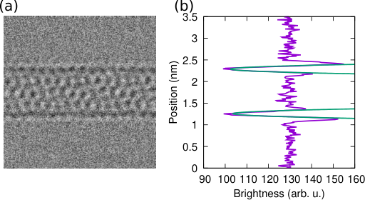
Before analyzing HRTEM images by the CNNs, they are processed first using the following procedure. In a first step, the images are oriented in such a way that the axis of the tubes are horizontally aligned. This is achieved by projecting the grayscale values of the images as a function of image orientation. The Fresnel fringes from the sides of the CNTs correspond to minima in the projection curves. The angle of the projection where the minima are deepest and narrowest aligns the tube (see Fig. 5).

In a second step, the images are downsampled to the image resolution used during the training of the CNN, i.e., 26.7 px/nm. From the rescaled images 40, 64 $\times$ 64 px subimages are cropped, normalized and equalized. These subimages are then processed first by the CNN that assigns them a particular class of diameter. After that, they are analyzed by the 40 instances of the CNN corresponding to the CNT diameter class determined by the first CNN. Finally, from the resulting total of 40 $\times$ 40 chirality estimates an overall chirality prediction is aggregated.

III.3 Evaluation of the classification system

The performance of the classification system is first evaluated using simulated HRTEM images. For this purpose, we take the entire system including the preprocessing stage and use 100 images of each of the considered chiralities containing the same variability as the training data. Figure 6, shows the rate of misclassification as a function of chiral angles and diameters. It turns out that the first CNN that determines the diameter class correctly classifies the image in over 99% of the cases, while the overall system reaches an accuracy of 90.5%, averaged over all chiralities. This means that most of the errors occur with the second CNN that assigns the final chiral indices. The overall system performs best for low diameter tubes. This tendency can be understood easily, because for low diameter tubes, there are less possible tubes in a given diameter range, and the possible chiral angles differ more between neighboring chiral indices.

For CNTs of larger diameters, misclassifications are more likely in the case of the near armchair tubes. The unit cells of CNTs tend to grow with diameter, and therefore in the individual small 64 $\times$ 64 px images that are the inputs for the CNNs, only a relatively small fraction of the moiré pattern is present which makes the classification task more difficult.

Figure 7: (Color online) Classification accuracy as a function of image quality percentile. Image quality is quantified as the contrast between the bright and dark fringes at the sides of the CNT.

Furthermore, it seems reasonable to assume that the image quality has an effect on the classification accuracy. In order to discuss this effect, the image quality of the 27100 images from the test set has been quantified. For this purpose, the ratio of the intensity of the bright and dark fringes at the sides of the tubes has been evaluated (see Fig. 5). Ordering the images by this measure of images quality, it turns out that the overall error rate can be reduced by taking into account only the images with the highest contrast between the dark and bright fringes. Figure 7 shows the classification accuracy of the overall system as a function of the percentile of the highest quality images. This emphasizes that the classification methodology relies on high quality images.

Figure 8(a-c), gives examples of images that resulted in correct classifications with high probability. Unsurprisingly, this occurs most often with images containing clear moiré patterns of CNTs with small diameters. In such cases, the result is very clear and allows unambiguous identification of the chirality of the considered tube. It is also instructive to examine individual cases where the classification system fails. In some cases, the system indicates high probabilities ( $>$ 95%) for a certain wrong chirality [see Fig. 8(d-f)]. Most of these misclassifications occur for structures with clearly visible defects and the predicted chiral index $n$ differs by only one unit from the true index. This type of error tends to occur more often with CNTs of larger diameter. Figure 8(g-h) shows examples of misclassifications where the differences between the predicted and true chiral indices are highest. These error cases occur when the first CNN that determines the diameter range of the CNT fails. In this case, the final analysis is carried out by a CNN that does not include the correct chirality in its classification range. Interestingly, most often, the wrong CNN will still select a chirality with a similar chiral angle as the one of the correct CNT. In these cases, the defocus mostly has rather extreme values, which makes the fringes at the sides of the CNTs as well as the moiré pattern less clear. These are conditions that makes the chirality assignment difficult also for human experts. It turns out, however, that this error mode never occurred when analyzing experimental HRTEM images [see Fig. 9(b)]. Several alternative approaches to programmatic chirality assignment are discussed in section S1.

The range of variations of geometrical aberrations used for the training of the CNNs may seem very narrow. Indeed, aberrations may change over time Barthel and Thust 2013 and oscillation of the sample under beam irradiation affects the focal distance Alloyeau et al. 2012. We assume thus that some experimental images analyzed in this work have been acquired with optical parameters slightly out of the ranges defined in Tab 1. It turns out that our classification system still works well rather far outside these ranges, as discussed in section S5. We presume that this is due to the fact that visually the effect of different aberration coefficients can be rather similar. Therefore, due to the randomization of aberration coefficients in our training set, extreme images, similar to the ones of section S5, are also included in our training data base.

IV Application to experimental HRTEM images

The performance of the classification system was then evaluated on experimental HRTEM images. CNTs were observed using an aberration corrected Jeol ARM 200F microscope operating at 80 kV. Images from three different samples were used: CVD-grown CNTs prepared based on the method described in Ref. Castan et al. 2017 using an iron catalyst, and two chirality-enriched samples obtained from a HiPCo sample (NoPo Nanotechnologies, Inc.) by the aqueous two-phase extraction method Subbaiyan et al. 2014; van Bezouw et al. 2018. In the following, we will first present the established manual approach to determine the structure of a CNT from the experimental images (adapted from Ref. Ghedjatti et al. 2017). Then we compare with the chiral index assignment by our automatic procedure.

First, the diameter of the nanotube was measured by extracting a contrast intensity profile perpendicular to the tube axis [see Fig. 9(a)]. According to image simulations, the diameter at Scherzer defocus is equal to the distance between the two inflection points between the dark and bright fringes on the sides of the CNT, meaning the midpoint between the minimum of the dark fringe, and the maximum of the subsequent bright fringe. A Fourier Transform (FT) of the HRTEM image is then used to determine the chiral angle ( $\theta$ ) of the nanotube as discussed in section S1 [see also Fig. 9(a)]. Considering the measured diameter and chiral angle values (including error bars), we can assign possible $(n,m)$ pairs for the CNT. Comparing the FT with a calculated diffraction pattern for these chiralities can help exclude some possibilities. To discriminate between the possible $(n,m)$ pairs, the HRTEM image is compared to image simulations of all the possible chiralities. The comparison of the moiré patterns leads to an unambiguous $(n,m)$ assignment.

For the automatic determination, a rectangular region of interest is selected from the experimental image which is then analyzed by the classification system. The results for the two methods were compared for a total of 91 CNT images. Only images of sufficient quality were used for this statistical analysis: images where nanotubes were not fully suspended, too contaminated or damaged, or where the focus and alignment conditions of the microscope did not allow the extraction of a readable FT, were not included.

The analytical process of manually determining the structure of a tube is of the order of 15 to 30 minutes. In comparison, depending on computing hardware, the analysis using the deep learning method is much faster and can be carried out without supervision. The resulting chiralities using both, the conventional and deep learning based chirality determination methods, is shown in Fig. 9(c,d), respectively, and the correlation of the classification methods is represented in Fig. 9(b). Cases where the two methods lead to identical results correspond to elements on the diagonal. Elements below and above the diagonal indicate images that have been classified as a chirality of a smaller and larger diameter with the deep learning method than with the manual method, respectively. Overall, the two methods lead to the same result in 71 $\%$ of cases. An example of a manual classification in a case where the two methods agree, is shown in Fig. 9(a). The individual results are given in section S2, some more successfully classified images in section S3, and an example where the automatic procedure fails in section S4. When there is a disagreement between the two methods, the chirality that was found conventionally is the second or third most probable chirality according to the deep learning tool in three out of four cases. In most of the error cases, the mismatch in chiralities is always minimal: if the manual technique gives an $(n,m)$ chirality, then the automatic technique will likely give (n $\pm$ 1,m), or (n,m $\pm$ 1). When removing the nanotubes for which the automatic method is indecisive (probability for the first chirality below 80 $\%$ ) from the data set, the agreement percentage goes up to 100 $\%$ .

V Conclusion

We have developed a robust and efficient tool to obtain in a very simple way the CNT chirality from raw HRTEM images. Based on a classification method using CNNs, the determination of the chirality of CNTs is fast enough to provide meaningful statistics on experimentally produced samples. An important and original point of our approach is the establishment of a large database obtained from atomic-scale simulations to train the CNNs. The consideration of defects makes the images of our training data base comparable to experimental data.

Such an easy-to-use tool will be of great interest to the CNT community in different research fields. A typical case is the lack of control of CNT chirality during synthesis, which is a major obstacle to the widespread use of CNTs in technological applications Yang et al. 2014; Amara and Bichara 2017; Magnin et al. 2018; Rao et al. 2018; Forel et al. 2019. This critically depends on the reliable analysis of the chirality distribution of CNT samples. Another approach to achieve chiral selectivity within CNT samples is to work on the subsequent processing and sorting of the raw material Arnold et al. 2006; Hersam 2008; Fagan 2019. Here again, the validation of the sorting methods requires a precise analysis in terms of chirality, which can be performed using our tool.

There is no doubt that our approach will be useful for other fields of research related to nanotubes but also in nanoscience more generally. The approach implemented can clearly be adapted to other nano-objects such as the structure of nanoparticles (pure, bimetallic, twins) Prunier et al. 2015, characterization of defects in 2D materials Mouhoub et al. 2020 or identification of stacking in Van der Waals heterostuctures Banhart et al. 2011; Rasool et al. 2015; Geim and Grigorieva 2013. In addition, the implementation of the new generation of so-called sub-angstrom low-voltage electron microscopes makes it possible to study radiation-sensitive materials at ultra-high resolution Cao et al. 2020. Our tool will be very beneficial for the analysis of the resulting large amount of very accurate data Shree et al. 2019. Our approach demonstrates the great potential of deep learning methods for the analysis of HRTEM images, and we hope that it will stimulate further developments in this direction, such as single image super resolution Lim et al. 2017, in the very near future. In contrast to super resolution in other domains, the relevant physics of nanoscale systems is essentially known and may be transferred to the deep learning model during training.

Acknowledgements.

The authors thank the METSA research network for giving access to the Cs-corrected TEM of the MPQ-Paris Diderot laboratory. The authors acknowledge M. Kociak (DiffractX) and Y. Le Bouar for use of their software, and S. Cambré, W. Wenseleers, and J. Defillet for providing part of the samples used for experimental images. This work benefited from the support of the project ANR GIANT (project 18-CE09-0014) of the French National Research Agency (ANR).

References

Iijima (1991) S. Iijima, “Helical microtubules of graphitic carbon,” Nature (London) 354, 56–58 (1991).
Popov (2004) V. N. Popov, “Carbon nanotubes: Properties and application,” Mater. Sci. Eng. R 43, 61–102 (2004).
Scarselli et al. (2012) M. Scarselli, P. Castrucci, and M. D. Crescenzi, “Electronic and optoelectronic nano-devices based on carbon nanotubes,” J. Phys.: Condens. Matter 24, 313202 (2012).
Rajter et al. (2013) R. F. Rajter, R. H. French, W. Y. Ching, R. Podgornik, and V. A. Parsegian, “Chirality-dependent properties of carbon nanotubes: Electronic structure, optical dispersion properties, hamaker coefficients and van der Waals–London dispersion interactions,” RSC Adv. 3, 823–842 (2013).
Hamada et al. (1992) N. Hamada, S. Sawada, and A. Oshiyama, “New one-dimensional conductors: Graphitic microtubules,” Phys. Rev. Lett. 68, 1579–1581 (1992).
Ding et al. (2017) E.-X. Ding, H. Jiang, Q. Zhang, Y. Tian, P. Laiho, A. Hussain, Y. Liao, N. Wei, and E. I. Kauppinen, “Highly conductive and transparent single-walled carbon nanotube thin films from ethanol by floating catalyst chemical vapor deposition,” Nanoscale 9, 17601–17609 (2017).
Tonkikh et al. (2019) A. A. Tonkikh, V. I. Tsebro, E. A. Obraztsova, D. V. Rybkovskiy, A. S. Orekhov, I. I. Kondrashov, E. I. Kauppinen, A. L. Chuvilin, and E. D. Obraztsova, “Films of filled single-wall carbon nanotubes as a new material for high-performance air-sustainable transparent conductive electrodes operating in a wide spectral range,” Nanoscale 11, 6755–6765 (2019).
Tans et al. (1998) S. J. Tans, A. R. M. Verschueren, and C. Dekker, “Room-temperature transistor based on a single carbon nanotube,” Nature (London) 393, 49–52 (1998).
Franklin et al. (2012) A. D. Franklin, M. Luisier, S.-J. Han, G. Tulevski, C. M. Breslin, L. Gignac, M. S. Lundstrom, and W. Haensch, “Sub-10 nm carbon nanotube transistor,” Nano Lett. 12, 758–762 (2012).
Shulaker et al. (2013) M. M. Shulaker, G. Hills, N. Patil, H. Wei, H.-Y. Chen, H.-S. P. Wong, and S. Mitra, “Carbon nanotube computer,” Nature (London) 501, 526 (2013).
Hills et al. (2019) G. Hills, C. Lau, A. Wright, S. Fuller, M. D. Bishop, T. Srimani, P. Kanhaiya, R. Ho, A. Amer, Y. Stein, D. Murphy, Arvind, A. Chandrakasan, and M. M. Shulaker, “Modern microprocessor built from complementary carbon nanotube transistors,” Nature (London) 572, 595–602 (2019).
Vialla et al. (2013) F. Vialla, C. Roquelet, B. Langlois, G. Delport, S. M. Santos, E. Deleporte, P. Roussignol, C. Delalande, C. Voisin, and J.-S. Lauret, “Chirality dependence of the absorption cross section of carbon nanotubes,” Phys. Rev. Lett. 111, 137402 (2013).
Kataura et al. (1999) H. Kataura, Y. Kumazawa, Y. Maniwa, I. Umezu, S. Suzuki, Y. Ohtsuka, and Y. Achiba, “Optical properties of single-wall carbon nanotubes,” Synth. Met. 103, 2555–2558 (1999).
Lefebvre et al. (2004) J. Lefebvre, J. M. Fraser, P. Finnie, and Y. Homma, “Photoluminescence from an individual single-walled carbon nanotube,” Phys. Rev. B 69, 075403 (2004).
Dresselhaus et al. (2005) M. S. Dresselhaus, G. Dresselhaus, R. Saito, and A. Jorio, “Raman spectroscopy of carbon nanotubes,” Phys. Rep. 409, 47–99 (2005).
Meyer et al. (2005) J. C. Meyer, M. Paillet, T. Michel, A. Moréac, A. Neumann, G. S. Duesberg, S. Roth, and J.-L. Sauvajol, “Raman modes of index-identified freestanding single-walled carbon nanotubes,” Phys. Rev. Lett. 95, 217401 (2005).
Wang et al. (2005) F. Wang, G. Dukovic, L. E. Brus, and T. F. Heinz, “The optical resonances in carbon nanotubes arise from excitons,” Science 308, 838–841 (2005).
Oyama et al. (2006) Y. Oyama, R. Saito, K. Sato, J. Jiang, G. G. Samsonidze, A. Grüneis, Y. Miyauchi, S. Maruyama, A. Jorio, G. Dresselhaus, and M. S. Dresselhaus, “Photoluminescence intensity of single-wall carbon nanotubes,” Carbon 44, 873–879 (2006).
Castan et al. (2018) A. Castan, S. Forel, F. Fossard, A. Ghedjatti, C. S. Cojocaru, V. Huc, and A. Loiseau, “Comparing TEM and resonant Raman spectroscopy for diameter distribution assessment of single wall carbon nanotubes,” (2018).
Sanchez et al. (2016) S. R. Sanchez, S. M. Bachilo, Y. Kadria-Vili, C.-W. Lin, and R. B. Weisman, “(n, m)-specific absorption cross sections of single-walled carbon nanotubes measured by variance spectroscopy,” Nano Lett. 16, 6903–6909 (2016).
Colomer et al. (2001) J.-F. Colomer, L. Henrard, P. Lambin, and G. Van Tendeloo, “Electron diffraction study of small bundles of single-wall carbon nanotubes with unique helicity,” Phys. Rev. B 64, 125425 (2001).
Kociak et al. (2002) M. Kociak, K. Suenaga, K. Hirahara, Y. Saito, T. Nakahira, and S. Iijima, “Linking chiral indices and transport properties of double-walled carbon nanotubes,” Phys. Rev. Lett. 89, 155501 (2002).
Kociak et al. (2003) M. Kociak, K. Hirahara, K. Suenaga, and S. Iijima, “How accurate can the determination of chiral indices of carbon nanotubes be?” Eur. Phys. J. B 32, 457–469 (2003).
Zuo et al. (2003) J. M. Zuo, I. Vartanyants, M. Gao, R. Zhang, and L. A. Nagahara, “Atomic resolution imaging of a carbon nanotube from diffraction intensities,” Science 300, 1419–1421 (2003).
Zhu et al. (2005) H. Zhu, K. Suenaga, A. Hashimoto, K. Urita, and S. Iijima, “Structural identification of single and double-walled carbon nanotubes by high-resolution transmission electron microscopy,” Chem. Phys. Lett. 412, 116–120 (2005).
Jiang et al. (2007) H. Jiang, A. G. Nasibulin, D. P. Brown, and E. I. Kauppinen, “Unambiguous atomic structural determination of single-walled carbon nanotubes by electron diffraction,” Carbon 45, 662–667 (2007).
Alemán et al. (2016) B. Alemán, M. M. Bernal, B. Mas, E. M. Pérez, V. Reguero, G. Xu, Y. Cui, and J. J. Vilatela, “Inherent predominance of high chiral angle metallic carbon nanotubes in continuous fibers grown from a molten catalyst,” Nanoscale 8, 4236–4244 (2016).
Zhang et al. (2016) F. Zhang, P.-X. Hou, C. Liu, B.-W. Wang, H. Jiang, M.-L. Chen, D.-M. Sun, J.-C. Li, H.-T. Cong, E. I. Kauppinen, and H.-M. Cheng, “Growth of semiconducting single-wall carbon nanotubes with a narrow band-gap distribution,” Nat. Commun. 7, 11160 (2016).
He et al. (2018) M. He, T. Yang, D. Shang, B. Xin, A. I. Chernov, E. D. Obraztsova, J. Sainio, N. Wei, H. Cui, H. Jiang, and E. Kauppinen, “High temperature growth of single-walled carbon nanotubes with a narrow chirality distribution by tip-growth mode,” Chem. Eng. J. 341, 344–350 (2018).
Haider et al. (1998) M. Haider, H. Rose, S. Uhlemann, E. Schwan, B. Kabius, and K. Urban, “A spherical-aberration-corrected 200kV transmission electron microscope,” Ultramicroscopy 75, 53–60 (1998).
Batson et al. (2002) P. E. Batson, N. Dellby, and O. L. Krivanek, “Sub-ångstrom resolution using aberration corrected electron optics,” Nature (London) 418, 617–620 (2002).
Hirahara et al. (2006) K. Hirahara, K. Saitoh, J. Yamasaki, and N. Tanaka, “Direct observation of six-membered rings in the upper and lower walls of a single-wall carbon nanotube by spherical aberration-corrected HRTEM,” Nano Lett. 6, 1778–1783 (2006).
Alloyeau et al. (2012) D. Alloyeau, T. Oikawa, J. Nelayah, G. Wang, and C. Ricolleau, “Following ostwald ripening in nanoalloys by high-resolution imaging with single-atom chemical sensitivity,” Appl. Phys. Lett. 101, 121920 (2012).
Warner et al. (2011) J. H. Warner, N. P. Young, A. I. Kirkland, and G. A. D. Briggs, “Resolving strain in carbon nanotubes at the atomic level,” Nat. Mater. 10, 958–962 (2011).
Ghedjatti et al. (2017) A. Ghedjatti, Y. Magnin, F. Fossard, G. Wang, H. Amara, E. Flahaut, J.-S. Lauret, and A. Loiseau, “Structural properties of double-walled carbon nanotubes driven by mechanical interlayer coupling,” ACS Nano 11, 4840–4847 (2017).
LeCun et al. (1998) Y. LeCun, L. Bottou, Y. Bengio, and P. Haffner, “Gradient-based learning applied to document recognition,” Proc. IEEE 86, 2278–2324 (1998).
Carleo et al. (2019) G. Carleo, I. Cirac, K. Cranmer, L. Daudet, M. Schuld, N. Tishby, L. Vogt-Maranto, and L. Zdeborová, “Machine learning and the physical sciences,” Rev. Mod. Phys. 91, 045002 (2019).
Touvron et al. (2019) H. Touvron, A. Vedaldi, M. Douze, and H. Jégou, “Fixing the train-test resolution discrepancy,” in Advances in Neural Information Processing Systems 32 (Curran Associates, Inc., 2019) pp. 8250–8260.
Modarres et al. (2017) M. H. Modarres, R. Aversa, S. Cozzini, R. Ciancio, A. Leto, and G. P. Brandino, “Neural network for nanoscience scanning electron microscope image recognition,” Sci. Rep. 7, 13282 (2017).
Trujillo et al. (2017) M. C. R. Trujillo, T. E. Alarcón, O. S. Dalmau, and A. Zamudio Ojeda, “Segmentation of carbon nanotube images through an artificial neural network,” Soft Comput. 21, 611–625 (2017).
Ziatdinov et al. (2017) M. Ziatdinov, O. Dyck, A. Maksov, X. Li, X. Sang, K. Xiao, R. R. Unocic, R. Vasudevan, S. Jesse, and S. V. Kalinin, “Deep learning of atomically resolved scanning transmission electron microscopy images: Chemical identification and tracking local transformations,” ACS Nano 11, 12742–12752 (2017).
Madsen et al. (2018) J. Madsen, P. Liu, J. Kling, J. B. Wagner, T. W. Hansen, O. Winther, and J. Schiøtz, “A deep learning approach to identify local structures in atomic-resolution transmission electron microscopy images,” Adv. Theory Simul. 1, 1800037 (2018).
Li et al. (2018) W. Li, K. G. Field, and D. Morgan, “Automated defect analysis in electron microscopic images,” npj Comput. Mater. 4, 36 (2018).
lam (22 Nov 2016) “Lammps website,” https://lammps.sandia.gov (22 Nov 2016).
Plimpton (1995) S. Plimpton, “Fast parallel algorithms for short-range molecular dynamics,” J. Comput. Phys. 117, 1–19 (1995).
Rao et al. (2018) R. Rao, C. L. Pint, A. E. Islam, R. S. Weatherup, S. Hofmann, E. R. Meshot, F. Wu, C. Zhou, N. Dee, P. B. Amama, J. Carpena-Nuñez, W. Shi, D. L. Plata, E. S. Penev, B. I. Yakobson, P. B. Balbuena, C. Bichara, D. N. Futaba, S. Noda, H. Shin, K. S. Kim, B. Simard, F. Mirri, M. Pasquali, F. Fornasiero, E. I. Kauppinen, M. Arnold, B. A. Cola, P. Nikolaev, S. Arepalli, H. M. Cheng, D. N. Zakharov, E. A. Stach, J. Zhang, F. Wei, M. Terrones, D. B. Geohegan, B. Maruyama, S. Maruyama, Y. Li, W. W. Adams, and A. J. Hart, “Carbon nanotubes and related nanomaterials: Critical advances and challenges for synthesis toward mainstream commercial applications,” ACS Nano 12, 11756–11784 (2018).
Tersoff (1989) J. Tersoff, “Modeling solid-state chemistry: Interatomic potentials for multicomponent systems,” Phys. Rev. B 39, 5566–5568 (1989).
Tersoff (1990) J. Tersoff, “Erratum: Modeling solid-state chemistry: Interatomic potentials for multicomponent systems,” Phys. Rev. B 41, 3248–3248 (1990).
Meunier et al. (1998) V. Meunier, L. Henrard, and P. Lambin, “Energetics of bent carbon nanotubes,” Phys. Rev. B 57, 2586–2591 (1998).
Berber et al. (2000) S. Berber, Y.-K. Kwon, and D. Tománek, “Unusually high thermal conductivity of carbon nanotubes,” Phys. Rev. Lett. 84, 4613–4616 (2000).
Magnin et al. (2014) Y. Magnin, G. D. Förster, F. Rabilloud, F. Calvo, A. Zappelli, and C. Bichara, “Thermal expansion of free-standing graphene: Benchmarking semi-empirical potentials,” J. Phys.: Condens. Matter 26, 185401 (2014).
Stukowski (2010) A. Stukowski, “Visualization and analysis of atomistic simulation data with ovito-the open visualization tool,” Modell. Simul. Mater. Sci. Eng. 18, 015012 (2010).
Cowley and Moodie (1957) J. M. Cowley and A. F. Moodie, “The scattering of electrons by atoms and crystals. I. A new theoretical approach,” Acta Crystallogr. 10, 609–619 (1957).
Barthel (2018) J. Barthel, “Dr. Probe: A software for high-resolution STEM image simulation,” Ultramicroscopy 193, 1–11 (2018).
Kirkland (2010) E. J. Kirkland, Advanced computing in electron microscopy (2010).
Weickenmeier and Kohl (1991) A. Weickenmeier and H. Kohl, “Computation of absorptive form factors for high-energy electron diffraction,” Acta Crystallogr., Sect. A: Found. Adv. 47, 590–597 (1991).
Ricolleau et al. (2012) C. Ricolleau, J. Nelayah, T. Oikawa, Y. Kohno, N. Braidy, G. Wang, F. Hue, L. Florea, V. Pierron Bohnes, and D. Alloyeau, “Performances of an 80–200 kv microscope employing a cold-feg and an aberration-corrected objective lens,” J. Electron Microsc. 62, 283–293 (2012).
Chollet (2015) F. et al. Chollet, “Keras,” https://keras.io (2015).
Srivastava et al. (2014) N. Srivastava, G. Hinton, A. Krizhevsky, I. Sutskever, and R. Salakhutdinov, “Dropout: A simple way to prevent neural networks from overfitting,” J. Mach. Learn. Res. 15, 1929–1958 (2014).
Barthel and Thust (2013) J. Barthel and A. Thust, “On the optical stability of high-resolution transmission electron microscopes,” Ultramicroscopy 134, 6–17 (2013).
Castan et al. (2017) A. Castan, S. Forel, L. Catala, I. Florea, F. Fossard, F. Bouanis, A. Andrieux-Ledier, S. Mazerat, T. Mallah, V. Huc, A. Loiseau, and C. S. Cojocaru, “New method for the growth of single-walled carbon nanotubes from bimetallic nanoalloy catalysts based on prussian blue analog precursors,” Carbon 123, 583–592 (2017).
Subbaiyan et al. (2014) N. K. Subbaiyan, S. Cambré, A. N. G. Parra-Vasquez, E. H. Hároz, S. K. Doorn, and J. G. Duque, “Role of surfactants and salt in aqueous two-phase separation of carbon nanotubes toward simple chirality isolation,” ACS Nano 8, 1619–1628 (2014).
van Bezouw et al. (2018) S. van Bezouw, D. H. Arias, R. Ihly, S. Cambré, A. J. Ferguson, J. Campo, J. C. Johnson, J. Defillet, W. Wenseleers, and J. L. Blackburn, “Diameter-dependent optical absorption and excitation energy transfer from encapsulated dye molecules toward single-walled carbon nanotubes,” ACS Nano 12, 6881–6894 (2018).
Yang et al. (2014) F. Yang, X. Wang, D. Zhang, J. Yang, D. Luo, Z. Xu, J. Wei, J.-Q. Wang, Z. Xu, F. Peng, X. Li, R. Li, Y. Li, M. Li, X. Bai, F. Ding, and Y. Li, “Chirality-specific growth of single-walled carbon nanotubes on solid alloy catalysts,” Nature (London) 510, 522–524 (2014).
Amara and Bichara (2017) H. Amara and C. Bichara, “Modeling the growth of single-wall carbon nanotubes,” Top. Curr. Chem. 375, 55 (2017).
Magnin et al. (2018) Y. Magnin, H. Amara, F. Ducastelle, A. Loiseau, and C. Bichara, “Entropy-driven stability of chiral single-walled carbon nanotubes,” Science 362, 212–215 (2018).
Forel et al. (2019) S. Forel, A. Castan, H. Amara, I. Florea, F. Fossard, L. Catala, C. Bichara, T. Mallah, V. Huc, A. Loiseau, and C.-S. Cojocaru, “Tuning bimetallic catalysts for a selective growth of SWCNTs,” Nanoscale 11, 4091–4100 (2019).
Arnold et al. (2006) M. S. Arnold, A. A. Green, J. F. Hulvat, S. I. Stupp, and M. C. Hersam, “Sorting carbon nanotubes by electronic structure using density differentiation,” Nat. Nanotechnol. 1, 60–65 (2006).
Hersam (2008) M. C. Hersam, “Progress towards monodisperse single-walled carbon nanotubes,” Nat. Nanotechnol. 3, 387–394 (2008).
Fagan (2019) J. A. Fagan, “Aqueous two-polymer phase extraction of single-wall carbon nanotubes using surfactants,” Nanoscale Adv. 1, 3307–3324 (2019).
Prunier et al. (2015) H. Prunier, J. Nelayah, C. Ricolleau, G. Wang, S. Nowak, A.-F. Lamic-Humblot, and D. Alloyeau, “New insights into the mixing of gold and copper in a nanoparticle from a structural study of Au–Cu nanoalloys synthesized via a wet chemistry method and pulsed laser deposition,” Phys. Chem. Chem. Phys. 17, 28339–28346 (2015).
Mouhoub et al. (2020) O. Mouhoub, R. Martinez-Gordillo, J. Nelayah, G. Wang, J.-H. Park, K. K. Kim, Y. H. Lee, C. Bichara, A. Loiseau, C. Ricolleau, H. Amara, and D. Alloyeau, “Quantitative insights into the growth mechanisms of nanopores in hexagonal boron nitride,” Phys. Rev. Materials 4, 014005 (2020).
Banhart et al. (2011) F. Banhart, J. Kotakoski, and A. V. Krasheninnikov, “Structural defects in graphene,” ACS Nano 5, 26–41 (2011).
Rasool et al. (2015) H. I. Rasool, C. Ophus, and A. Zettl, “Atomic defects in two dimensional materials,” Adv. Mater. 27, 5771–5777 (2015).
Geim and Grigorieva (2013) A. K. Geim and I. V. Grigorieva, “Van der Waals heterostructures.” Nature (London) 499, 419–25 (2013).
Cao et al. (2020) K. Cao, S. T. Skowron, J. Biskupek, C. T. Stoppiello, C. Leist, E. Besley, A. N. Khlobystov, and U. Kaiser, “Imaging an unsupported metal–metal bond in dirhenium molecules at the atomic scale,” Sci. Adv. 6 (2020), 10.1126/sciadv.aay5849.
Shree et al. (2019) S. Shree, A. George, T. Lehnert, C. Neumann, M. Benelajla, C. Robert, X. Marie, K. Watanabe, T. Taniguchi, U. Kaiser, B. Urbaszek, and A. Turchanin, “High optical quality of MoS2 monolayers grown by chemical vapor deposition,” 2D Mater. 7, 015011 (2019).
Lim et al. (2017) B. Lim, S. Son, H. Kim, S. Nah, and K. Mu Lee, “Enhanced deep residual networks for single image super-resolution,” in The IEEE Conference on Computer Vision and Pattern Recognition (CVPR) Workshops (2017) arXiv:1707.02921 .