Design of pseudo-mechanisms and multistable units for mechanical metamaterials
Abstract
Mechanism—collections of rigid elements coupled by perfect hinges which exhibit a zero-energy motion—motivate the design of a variety of mechanical metamaterials. We enlarge this design space by considering pseudo-mechanisms, collections of elastically coupled elements that exhibit motions with very low energy costs. We show that their geometric design generally is distinct from those of true mechanisms, thus opening up a large and virtually unexplored design space. We further extend this space by designing building blocks with bistable and tristable energy landscapes, realize these by 3D printing, and show how these form unit cells for multistable metamaterials.
pacs
81.05.Xj, 81.05.Zx, 45.80.+r, 46.70.-pA mechanism is a collection of flexibly linked, rigid elements which exhibits a zero-energy motion. Mechanisms play a foundational role in the physics of jammed media and spring networks alexander; network1; network2; network3; network4; jam1; jam2, and are central in mechanical engineering, where they underlie the design of robotic devices such as grippers robot; Detweiler. Imperfect mechanisms, based on distorted geometries Dudte:2016db; Jesse; Stern:2017bya; Meeussen, extra bonds/connections alexander; network1; network2; network3; network4; jam1; jam2, or non-ideal hinges natphyschain frequently occur, and these exhibit soft modes similar to the zero energy motions of the underlying mechanism. In particular, mechanism-based metamaterials borrow the geometric design of mechanisms but replace the hinges by slender, flexible parts which connect stiffer elements, such that the soft modes of the metamaterial are similar to the free motion of the underlying mechanism. External forces easily excite these soft modes, and as the mechanism-derived soft modes can be very different from those of ordinary elastic modes, exotic properties may emerge review, including negative response parameters auxetic; katia; Reid, shape-morphing cube; Overvelde:2017; Chiara; kimnatphys, topological polarization Jayson; Chen:2016bk; Marc; zeb, programmability and multistability Jesse; bastiaan; Waitukaitis:2015dk; Dudte:2016db; rafsanjani and (self-)folding Overvelde:2017; Chen:2016bk; Jesse; Waitukaitis:2015dk; Dudte:2016db; Filipov:2015; Stern:2017bya; Filipov:2017; sequential; Stern:2018; Chen:2019; natphysori.
However, as mechanism-based metamaterials do not have true zero modes review; natphyschain, the design of a flexible metamaterial does not require an underlying true zero-energy mechanism. This suggests to consider pseudo-mechanisms (PMs), which we define as collections of flexibly coupled rigid elements that exhibit motions with (very) low energy costs.
Here we show that PMs are widespread, by constructing a quadrilateral based PMs by use of particle swarm optimization. Our central finding is that most PMs are geometrically very distinct from true mechanisms; most PMs are not simply perturbed mechanisms, but PMs permeate the design space very far away from the true mechanism subspace. We extend our search techniques to obtain multistable units rafsanjani, and bring these to life using 3D printing. Finally, we show how to tile our unit cells to obtain complex periodic metamaterials. Together, our approach, which is computationally effective, suggests new avenues for the design of shapemorphing and multistable metamaterials review as well as devices for robotics or deployable structures such as bellows robot; deploy.
System.— We consider collections of quadrilaterals connected in a square topology by hinges with zero torsional stiffness and finite stretchability (Fig. 1). For equally sized squares, such system has a zero-mode and is known as the rotating square mechanism grima; this geometry underlies a large number of mechanical metamaterials review; katia; cube; Chiara; bastiaan; sequential; natphyschain; luuk. Generalizations, including to regular tilings of alternatingly sized squares, rectangles or 3D, are well known cube; bastiaan; Finish_dude; kirisq. The condition for such collections of quadrilaterals to form a mechanism are simple. For definiteness, we focus on tilings of quadrilaterals (Fig. 1a). We can consider such tilings as collections of connected four-bar linkages , and then express the relations between their (inner) angles by mappings . It can be shown that quadrilateral tilings can only form a mechanism if all four-bar linkages (voids) form parallelograms, as these are associated with linear mappings geom. In contrast, for generic quadrilaterals the mappings are nonlinear, and tilings of (or larger) generic quadrilaterals do not poses a zero energy motion geom; luuk; MC (Fig. 1a).
To make progress, we focus on a diluted unit, obtained by removing quadrilateral 9, which yields a mechanism with a freely hinging, zero energy, finite amplitude mode luuk; MC (Fig. 1b). To characterize this mechanism, we remove all extraneous information, and replace the corner quadrilaterials with rigid bars (Fig. 1b). The geometry of this mechanism is specified by the coordinates of the 12 links , which span a 24 dimensional design space. We control the free motion of this mechanism by , the deviation of from its initial value, and characterize the diluted unit by as function of (Fig. 1b). Experimentally, stretching or compressing two points on the systems, or compressing it between parallel plates actuates the soft mode of the system that we describe here. The function acts as a proxy for the mechanics of a full unit consisting of flexible elements: if is a constant, reinserting a ninth quad of appropriate dimensions yield a full unit with a zero mode MC; note1 Fig. 1c(i). For nearly constant , reinserting the ninth quadrilateral would lead to a system with a large amplitude motion with a very low energy: a pseudo-mechanism. For generic quadrilaterals is a nonlinear function (Fig. 1c(ii-iii)), and inserting the ninth quadrilateral yields a more complex energy landscape. The design problem is thus to obtain coordinates so that closely matches a target function .

Design by particle swarm optimization.— We define a cost function based on the normalized Euclidean distance between and , combined with discrete constraints to avoid non-fitting quadrilaterals, overlapping quadrilaterals, and designs where the quadrilateral sizes differ too much (see S.I.). Exploring this design space requires an algorithm that does not easily get stuck in shallow minima, as purely gradient based methods would. Evolutionary algorithms are eminently suited for this, and we choose here to use particle swarm optimization (PSO) due to its simplicity and ease of tuning. This method employs an ensemble (swarm) of particles - each representing a particular design - and is known to allow to identify deep minima in a rugged landscape pso1; pso2; pso3; pso4; pso5; pso6; pso7. While we note that our approach remains valid for larger structures, the computational time grows exponentially in the size of the structure and we focus here on structures. The PSO algorithm keeps track of the best position discovered by each particle up to generation (iteration) , , and by the best position discovered by all the particles — the swarm — . We seed an initial population of randomly distributed particles with random velocities. During the search, each particle is attracted towards a stochastic mix of and :
| (1) | |||||
| (2) |
where and are random vectors whose elements are uniformly distributed between 0 and 1, and the so-called inertia , cognition and social hyper-parameters must be chosen to optimize convergence. For our specific design problem, the position and velocity of particle i are both 24-dimensional vectors, and we have verified by hyper-parameter optimization that the algorithm yields good results for , , and (see SI). For each target function, we run 3000 runs for each of the 36 pairs of parameter values that satisfy , and , leading to a total of runs. For details, see the Supplemental Information.

Generic flexible unit cells.— We first focus on designing diluted units for which is close to a constant. We set the target curve and deploy PSO to obtain designs with low values of . We find a large number of designs for which is very small, so that is close to a constant (Fig. 2). We quantify the geometry of these solutions through an order-parameter, , which measures the proximity of the four internal four-bar linkages to parallelogram linkages. We define for the linkage as
| (3) |
where are the bar lengths of linkage , and define as
| (4) |
While our algorithm finds some solutions with small , i.e., close to the true mechanism limit where all linkages are parallelograms (Fig. 2a), the vast majority of solutions with low have significantly larger values of (Fig. 2b-c). Notwithstanding this strong deviation from true mechanisms, the peak deviation between and can be as small as (Fig. 2d-f).
We show a scatter plot of versus , and the individual distributions of and — which are only weakly correlated — in Fig. 2g-i. These plots reveal that the distribution of is log-normal, with normally distributed with the center at , corresponding to designs that are very far away from strict mechanisms (). Hence, pseudo-mechanisms with anomalously low functional deviations from true mechanisms are widespread, and occur in regions of design space that are far away from true mechanisms.
Our findings suggest a complex organization of the design space. To gain insight into this structure, we have explored whether the value of increases if a certain solution is randomly perturbed. Specifically, we generate 1000 random 24 dimensional vectors with each entry uniformly distributed between -1 and 1, and then calculate for a range of . For the deep solution, where , we find that all , consistent with the idea that these solutions are local minima (see S.I.). In contrast, for solutions with much larger values of we find a small but finite probability that for small perturbations () but not for larger perturbations of order . We suggest that these solutions perhaps are close to a shallow local minimum, and note that PSO is not guaranteed to find local minima with high accuracy (For details, see S.I.).
Multistable unit cells.— The ease with which we can find pseudo mechanisms prompts the question if it is similarly easy to generate designs for other target functions. For systems with flexible hinges, inserting a ninth quad with dimension provides the blueprint for a unit with low energy states for , so that nonmonotonic lead to multi-stable structures. We have investigated four families of target functions, ; ; and , for a range of values of between and thesisnitin. Here we focus on the designs for and , as these form the basis for bistable and tristable units.
We show scatter plots of vs for and in Fig. 3, for . We observe a large cloud of solutions, and note that the typical values of for curves with more extrema are somewhat larger than those for . Examples of designs of diluted units that closely satisfy the target curves are shown in Fig. 3.
We experimentally realized full units based on the designs shown in Fig. (3b,g), by adding a ninth quad of appropriate length, and then 3D printing these units with flexible material (filaflex). The out-of-plane thickness of these sample is 10 mm and the connecting hinges have a minimum thickness of 0.5 mm. Despite the finite flexibility of all quads, and the finite but small bending stiffness of their hinges, we observe that these samples are indeed bistable and tristable respectively, with their stable configurations close to the expected configurations (Fig. 3d,e,j,k,l).

Complex Tilings.— Finally, we briefly outline how we can connect complex units into larger systems. Each PM can be augmented by replacing the outer bars by triangles (Fig. 4a-b). The outer tips of this unit form a quadrilateral, and as any quadrilateral can be tiled in a pattern where adjacent quadrilaterals are rotated by , larger PMs can readily be designed by connecting these units (Fig. 4c). One can similarly augment multistable unit cells, and for a tiling of general augmenting triangles one expects stable collective states only when all units are in the same configuration, as the ‘gap’ distance between tips of triangles generally differs in different minima. However, the augmenting triangles can be chosen such that this gap has the same length in each stable state (Fig. 4d-e). Connecting such augmented units in a tiling yields a design with energy minima when each individual unit is in its stable state, leading to a number of stable states which grows exponentially with system size (Fig. 4f-i).
Summary and Outlook.— We have presented a novel strategy for the design of metamaterial architectures, based on pseudo-mechanisms which can have a geometric structure which is surprisingly far removed from that of strict mechanisms. As similar pseudo-mechanisms can be observed in 2D origami, where PMs allow to circumvent the difficult design of rigidly folding mechanisms Dudte:2016db; Stern:2017bya; Stern:2018; natphysori, we speculate that pseudo-mechanisms are generic and relevant for a wide classes of structures, including networks of hinged bars kimnatphys and (3D) origami Overvelde:2017. Moreover, the ease of designing multistable structures in a hierarchical fashion—coupling complex units in tilings—suggest to generalize this approach to other classes also.
Extensions of our work include the design of larger non-periodic collections of quadrilaterals that form pseudo-mechanisms. Conceptually, the step from a mechanism to a pseudo mechanism might be similar to that from a to a pseudo mechanism, but it is an open question how the design space evolves for increasingly large systems. A further intriguing possibility arises for, e.g., bellows: while the volume of a polyhedron cannot change as it flexes, pseudo-mechanisms may in practice work equally well deploy. Moreover, we wonder whether pseudomechanisms can mimic an equivalent of the topological polarization, edge-modes and corner-modes observed in topologically non-trivial mechanical metamaterials that are based on true mechanisms Jayson; Chen:2016bk; Marc; zeb. Finally, our designs space is only of moderate dimensions, and obtaining nontrivial designs is computationally relatively cheap. This makes our designs eminently suited to test whether machine learning techniques would be suitable to, first, be trained to distinguish “good” from “bad” pseudo mechanisms, second, to detect and classify multistable designs, and third, can be used to speed up the design of such structures MLori; bessa.
Acknowledgements.— We thank M. Bessa, M. Dijkstra, S. Guest, A. Murugan, S. Pellegrino and T. Tachi for productive discussions. This work is part of an Industrial Partnership Programme of the Netherlands Organization for Scientific Research (NWO) under grant nr 12CSER036.
References
- (1) S. Alexander, Phys. Rep. 296, 65 (1998).
- (2) W. G. Ellenbroek, Z. Zeravcic, W. van Saarloos, and M. van Hecke, Europhys. Lett. 87, 34004 (2009).
- (3) W. G. Ellenbroek, V. F. Hagh, A. Kumar, M. F. Thorpe, and M. van Hecke, Phys. Rev. Lett. 114, 135501 (2015).
- (4) C. P. Goodrich, A. J. Liu and S. R. Nagel Phys. Rev. Lett. 114, 225501 (2015).
- (5) J. W. Rocks, N. Pashine, I. Bischofberger, C. P. Goodrich, A. J. Liu, and S. R. Nagel, Proc. Natl. Acad. Sci. 114, 2520 (2017).
- (6) A. J. Liu and S. R. Nagel, Annu. Rev. Condens. Matter Phys. 1, 347 (2010).
- (7) M. van Hecke, J. Phys. Condens. Matter 22, 033101 (2010).
- (8) C. Detweiler, M. Vona, Y. Yoon, S.-K. Yun and D. Rus, IEEE Robotics Autom. Mag. 14, 4555 (2007).
- (9) D. Rus and M. T. Tolley, Nature 521, 467 (2015).
- (10) J. L. Silverberg et al.. Science 345,647 (2014)
- (11) L.H. Dudte, E. Vouga, T. Tachi, and L. Mahadevan, Nat. Mater. 15, 583-589 (2016).
- (12) M. Stern, M.B. Pinson, and A. Murugan, Phys. Rev. X 7, 041070 (2017).
- (13) A. Meeussen, E. C. Oguz, Y. Shokef and M van Hecke, Nat. Phys. https://doi.org/10.1038/s41567-019-0763-6 (2020).
- (14) C. Coulais, C. Kettenis and M. van Hecke, Nat. Phys. 14 40 (2018).
- (15) A. Rafsanjani and D. Pasini, Extr. Mech. Let. 9, 291 (2016).
- (16) K. Bertoldi, V. Vitelli, J. Christensen and M. van Hecke, Nat. Rev. Mater. 2, 17066 (2017).
- (17) R. S. Lakes, Science 235, 1038 (1987).
- (18) T. Mullin, S. Deschanel, K. Bertoldi, and M. C. Boyce, Phys. Rev. Lett. 99, 084301 (2007).
- (19) D. R. Reid et al. Proc. Natl. Acad. Sci. 115, 1384 (2018).
- (20) C. Coulais, E. Teomy, K. de Reus, Y. Shokef and M. van Hecke, Nature 535 529 (2016).
- (21) J.T.B. Overvelde, J.C. Weaver, C. Hoberman, and K. Bertoldi, Nature 541, 347-352 (2017).
- (22) P. Celli et al., Soft Matter 14, 9744 (2018).
- (23) J. Z. Kim, Z. X. Lu, S. H. Strogatz, and D. S Bassett, Nat. Phys. 15, 714 (2019).
- (24) J. Paulose, B. G.-g. Chen and V. Vitelli, Nat. Phys. 11, 153 (2015).
- (25) B.G.-g. Chen et al., Phys. Rev. Lett. 116, 135501 (2016).
- (26) D. Z. Rocklin, S. Zhou, K. Sun, X. Mao, Nat. comm. 8, 14201 (2017).
- (27) M. Serra-Garcia et al., Nature 555, 342 (2018).
- (28) B. Florijn, C. Coulais and M. van Hecke, Phys. Rev. Lett. 113, 175503 (2014).
- (29) S.R. Waitukaitis, R. Menaut, B.G.-g. Chen, and M. van Hecke, Phys. Rev. Lett. 114, 055503 (2015).
- (30) E.T. Filipov, T. Tachi and G.H. Paulino, Proc. Natl. Acad. Sci. 112, 12321-12326 (2015).
- (31) E.T. Filipov, K. Liu, T. Tachi, M. Schenk and G.H. Paulino, Int. J. Sol. Structs. 124, 26-45 (2017).
- (32) C. Coulais, A. Sabbadini, F. Vink and M. van Hecke, Nature 561, 512 (2018).
- (33) M. Stern, V. Jayaram, A. Murugan, Nat. Comm. 9, 4303 (2018).
- (34) S.H. Chen, L. Mahadevan, Proc. Natl. Acad. Sci. 116, 8119-8124 (2019).
- (35) P. Dieleman, N. Vasmel, S. Waitukaitis and M. van Hecke, Nat. Phys. 16, 63 (2020).
- (36) I. K. Sabitov, Discrete Comput. Geom. 20, 405 (1998).
- (37) J. N. Grima and K. E. Evans J. Mater. Sci. Lett. 19, 1563 (2000).
- (38) L. A. Lubbers and M. van Hecke, Phys. Rev. E 100 021001R (2019).
- (39) D. Rayneau-Kirkhope, C. Zhang, L. Theran and M. A. Dias, Proc. Roy. Soc. A 474, 20170753 (2018).
- (40) Y. Tang et al., Adv. Mat. 27, 7181 (2015).
- (41) Yang Y., You Z. Journal of Mechanisms and Robotics, 10.2, 021001 (2018).
- (42) C. R. Calladine, Int. J. Sol. Struct 14, 161 (1978).
- (43) Consistent with Maxwell-Calladine counting, such a mechanism posseses an associated state of self-stress MC.
- (44) J. Kennedy and R. Eberhart. In: Proc. IEEE Int. Conf. Neural Networks, 1942 (1995).
- (45) R. Poli, J. Kennedy, and T. Blackwell. Swarm Intell. 1, 33 (2007).
- (46) R. C. Eberhart and Y. H. Shi, Special issue on particle swarm optimization, IEEE Trans. Evol. Comp. 8, 201 (2004).
- (47) A. Chatterjee and P. Siarry. Comp. Oper. Res. 33, 859 (2006).
- (48) A. Nickabadi, M. M. Ebadzadeh, and R. Safabakhsh. App. Soft Comp. 11, 3658 (2011).
- (49) M. Pant, R. Thangaraj, and A. Abraham. Found. of Comp. Intell. 3, 101 (2009).
- (50) A. L. Gutierrez, M. Lanza, I. Barriuso, L. Valle, M. Domingo, J. R. Perez, and J. Basterrechea, In: Ant. and Prop. (EUCAP), 5, 965 Springer (2011).
- (51) N. Singh, Strategies for mechanical metamaterial design, PhD Thesis (2019). DOI: http://hdl.handle.net/1887/71234.
- (52) P. Z. Hanakata, E. D. Cubuk, D. K. Campbell and H. S. Park, Phys. Rev. Lett. 121, 255304 (2018).
- (53) M. A. Bessa, P. Glowacki and M. Houlder, Adv. Mater. 31, 1904845 (2019).
I Supplemental Information
I.1 Objective function
We couple the rigid quads with springs of zero restlength and unit stiffness, and for given minimize the elastic energy with standard conjugate gradient techniques (to essentially zero) to obtain — this method makes it easy to deal with problems that may occur when some quadrilaterals grow too large or too small and are no longer able to connect to their neighbors. We define the objective function as the sum of the normalized Euclidean distance between and (), and three constraints (): Here is defined as , where =.
Disconnect constraint .— When some quadrilaterals grow too large or too small and are no longer able to connect to their neighbors, the energy cannot equilibrate to zero. We have found that for our numerical precision, for proper systems. We define for each a penalty when , otherwise, and define .
Overlap constraint .— During optimization, the evolving design variables may result in systems where some quadrilaterals overlap during their hinging motion. We identify such self-intersecting systems by first defining: (i) the outermost polygon , defined by its corners , (ii) the ‘windmill-shaped’ polygon , which encloses the four linkages and quadrilateral 5, and is defined by its corners and (iii) the inner polygon defined by , i.e., quadrilateral 5. The necessary and sufficient conditions to guarantee a non self-intersecting system are: (i) is ‘contained within’ , and (ii) all three , and are simple and do not self-intersect.
Similar as above, we need to check for the violation of the present constraint for every step of . Its value at the step is denoted by . A simple binary quantification for is implemented, where it is assigned a value 1 if self-intersection occurs and 0 otherwise. The total violation for the complete range of is given by :
| (5) |
Finally we note that can only be calculated if = 0. For , is simply assumed to be zero, and the constraint is sufficient to suppress such solutions
Size constraint .— We occasionally observe that, driven by penalties and , systems with disproportionate sizes of their quadrilaterals arise. In order to avoid such systems, we impose a third constraint whose aim is to keep every edge length of every polygon within a desired range between and . For each edge with length of each polygon we specify a minimum length and a maximum edge length , and assign a penalty by a piecewise linear function: for ; for ; for ; for . The total penalty is the sum
| (6) |
The typical magnitude of these three constraints during violations is significantly larger than the Euclidean distance between and , and as a result the collections of quadrilaterials obtained by our PSO algorithm satisfy these constraints and are bound in size, remain connected during hinging, and do not overlap.
I.2 Particle Swarm Optimization
Here we briefly summarize some of the technical details of our implementation of PSO.
Position initialization –
The search procedure begins by spreading the particles throughout search space [48, 49]. For each PSO particle, we first place the coordinates corresponding to a rotating square mechanism where each quadrilateral has a diagonal of length 1.5, and then perturb each of the 24 coordinates of with random numbers uniformly distributed between and . We then check whether any constraint is violated, and if so, generate a new particle, until all particles satisfy all constraints.
Velocity initialization.— We initialize the velocity of each particle in each dimension by a random number uniformly distributed between 0 and 1.
Swarm size.— The number of particles in the swarm aims to strike a balance between good coverage of the search space and computational efficiency. We found that for our problem a swarm size of 50 is adequate.
Termination criteria.— We terminate the PSO search when the number of iterations reaches 100.
I.3 Hyper-parameter Optimization
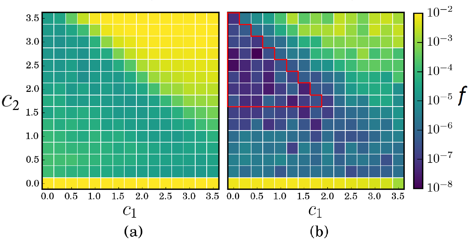
In PSO, the inertia , cognition and social hyper-parameters need to be chosen according to the underlying optimization problem, and we have performed a grid search method to gain insight into their role. For each value of these, we run 100 instances of the PSO method and keep track of both the mean and lowest value of the objective function. In Fig. 5 we show the results for and a range of and values. From this data we deduce the optimum hyperparameter subspace for as a triangular area in parameter space where , and . Similar studies for larger yield slightly smaller optimal subspaces, while significant lowering of also does not increase performance [49,50] — we thus fix and keep , and .
I.4 Local Minima Check
PSO discovers many realizations with very low objective function values. To explore the objective function landscape, we sample the variation of the objective value in the vicinity of such solutions. Specifically, we start from the final solution shown in Fig. 2b, generate 1000 random 24-dimensional vectors with each entry uniformly distributed between -1 and 1, and then calculate the cumulative distribution functions (CDFs) of for ranging from to . In all cases we find that (Fig. 6) While this is no proof that corresponds to a true local minimum, it strongly indicates that — within an accuracy of — is a good solution of the PSO algorithm. We note that a similar analysis for a solution with a much higher value of does not strictly satisfy (Fig. 7).