跳到论文正文
W Papers独立论文阅读器 arXiv:2003.11195 论文正文 计算阅读时间 · 0%
引用这篇论文根据当前论文元数据生成,正式投稿前建议核对。


License: arXiv.org perpetual non-exclusive license
arXiv:2003.11195v1 [cs.IT] 25 Mar 2020

Robust and Secure Beamforming for Intelligent Reflecting Surface Aided mmWave MISO Systems

Xingbo Lu    Weiwei Yang    Xinrong Guan    Qingqing Wu    Yueming Cai Thanks: This work was supported by the Natural Science Foundations of China (No. 61671474 and No. 61671939). X. Lu, W. Yang, X. Guan and Y. Cai are with Army Engineering University of PLA, Nanjing 210007, China. Q. Wu is with the Department of Electrical and Computer Engineering, National University of Singapore, Singapore 117583. (Email: xblu1221@126.com, wwyang1981@163.com, geniusg2017@gmail.com, elewuqq@nus.edu.sg, caiym@vip.sina.com. Corresponding author: Weiwei Yang.)
Abstract

In this letter, we investigate the robust and secure beamforming (RSBF) in an intelligent reflecting surface (IRS) aided millimeter wave (mmWave) multiple input single output (MISO) system, where multiple single antenna eavesdroppers (Eves) are arbitrarily distributed nearby the legitimate receiver. Considering the channel state information (CSI) of Eves’ channels is imperfectly known at the legitimate transmitter, the RSBF design problems to maximize the worst case of achievable secrecy rate (ASR) are formulated under the total transmission power and unit-modulus constraints. Since the problems are difficult to solve optimally due to their nonconvexity and coupled variables, we substitute the wiretap channels by a weighted combination of discrete samples and propose a RSBF scheme based on alternating optimization and semidefinite relaxation (SDR) techniques, for both colluding and noncolluding eavesdropping scenarios. Simulation results show that the proposed RSBF scheme can effectively improve the ASR and also outperforms other benchmark schemes.

Index Terms: 
Intelligent reflecting surface, millimeter wave, robust beamforming, physical layer security.

I Introduction

Millimeter wave (mmWave) communication has been considered as a promising technology for next generation wireless communication systems, due to its abundant spectrum and thus unrivaled data rates [1]. However, the substantial propagation loss renders the signals at mmWave band highly susceptible to be blocked by obstacles, thus resulting in a short coverage range. To address this issue, massive array antennas can be deployed, which, however, lead to unaffordable hardware cost and power consumption [2]. Recently, intelligent reflecting surface (IRS) has emerged as a promising technology to achieve high spectrum efficiency in a cost-effective manner [3]-[6]. Specifically, IRS is a software-controlled metasurface composed of a large number of reconfigurable and passive reflecting elements whose phase shift can be adaptively adjusted by a smart controller. By smartly adjusting the reflection coefficients, the reflected signals can be enhanced or weakened at different receivers. Due to the significant passive beamforming gain, IRS can be incorporated into the mmWave communication systems to extend the coverage and reduce the need for radio frequency (RF) chains [5] [7].

On the other hand, physical layer security (PLS) has been intensively investigated in recent years due to its capability of enhancing traditional secrecy system from the perspective of information theory. Since the IRS is able to configure the wireless channel in real-time via passive reflection, it has great potential in improving the secrecy rate [8]-[10]. Specifically, an IRS-aided secure single user multiple input single output (MISO) system was investigated in [8]. By adaptively adjusting the IRS’s phase shifts, the received signal at Bob is constructively strengthened but severely weakened with that at Eve, even though the legitimate and wiretap channels are highly correlated. An artificial-noise-aided secure wireless transmission scheme were proposed in the IRS-aided MIMO communication systems [9]. The multiple Eves scenario was extended in [10], in which the active beamforming (BF) vector with jamming and passive BF vector were jointly optimized to maximize the achievable secrecy rate (ASR).

Refer to caption
Fig. 1: System model.

Note that all aforementioned works about IRS-aided PLS are based on the assumption that the channel state information (CSI) of Bob and Eves’ channels is perfectly known at the legitimate transmitter. In practice, the CSI acquisition is one of the main challenges for IRS-aided systems due to the lack of RF chains at the IRS. In response this, channel estimation schemes based on element-wise on/off [11], near-orthogonal reflection pattern [12] and compressive sensing [13] have been proposed. However, it is almost impossible to acquire the perfect CSI of Eves’ channels even though Eves are assumed to be unscheduled active users in the network. To the best of our knowledge, there is no work considering such problem in IRS-aided mmWave secrecy communication systems. This motivates us to propose a robust BF scheme against the imperfect CSI of Eves’ channels. Specifically, assuming that multiple single antenna Eves are stochastically distributed nearby Bob and the angle of arrival (AoA)-based CSI of Eves’ channels is imperfectly known at Alice, we formulate robust secure beamforming (RSBF) problems to maximize the worst case ASR against non-colluding and colluding Eves, respectively. Since the formulated problems are non-convex and difficult to solve optimally, we express the wiretap channel based on the weight combination of discrete samples to deal with the imperfect CSI of Eves’ channels and then transform the problems into convex forms by applying semidefinite relaxation (SDR) technique. An efficient alternating optimization based RSBF scheme is proposed to solve them sub-optimally. Simulation results show that the proposed RSBF scheme can significantly improve the worst case ASR as compared to the benchmark schemes.

Notations: Throughout our discussions, the distribution of complex Gaussian random variable with mean υ\upsilon and variance σ2{\sigma^{2}} is denoted by 𝒞​𝒩​(υ,σ2){\mathcal{C}\mathcal{N}}\left(\upsilon,\sigma^{2}\right). [x]+=max⁡(0,x){\left[x\right]^{+}}\!\!=\!\max\left({0,x}\right). Superscript 𝐀T{{\bf{{A}}}^{T}}, 𝐀H{{\bf{{A}}}^{H}} and 𝐀−1{{\bf{{A}}}^{-1}} respectively denote the transpose, the conjugate transpose and the inverse of a matrix 𝐀{\bf{{A}}}. 𝐀​≻¯​0{\bf{A}}\underline{\succ}0 denotes that 𝐀{\bf{A}} is positive semi-definite. ⊗\otimes represents Kronecker product. e​i​g​(⋅)eig\left(\cdot\right) denotes the normalized eigenvector corresponding to the largest eigenvalue of the matrix. ‖⋅‖{\left\|\cdot\right\|}, t​r​(⋅)tr(\cdot) and ℂM×N{\mathbb{C}^{M\times N}} denote norm, the trace of a matrix and the space of M×NM\!\times\!N complex-valued matrices, respectively.

II System Model and Problem Formulation

II-A System Model

As shown in Fig. 1, we consider a mmWave secrecy communication system, where Alice intends to send confidential information to Bob in the presence of KK arbitrarily distributed Eves. Assuming the direct link between Alice and Bob is blocked by obstacles, an IRS managed by a smart controller is deployed to create a line-of-sight (LoS) path to serve Bob. Considering that Bob and Eves are all equipped with single antenna, while Alice and IRS are equipped with MM antennas and a uniform array with NN elements where Na​zN_{az} in horizon and Ne​lN_{el} in vertical, respectively.

The mmWave channels from Alice to IRS, IRS to Bob and the kk-th Eve are respectively denoted by 𝐇A​R{{\bf{H}}_{AR}}, 𝐡R​B{{\bf{h}}_{RB}} and 𝐡R​Ek{{\bf{h}}_{{RE}_{k}}}, which can be expressed as [1]

𝐇A​R=1/(βR​LR)​∑l=0LR−1αR​l​𝐚A​(M,ϕl)​𝐚RT​(N,θa​l,φa​l),\small{{\bf{H}}_{AR}}\!\!=\!\!\sqrt{1/\!\left({{\beta_{R}}{L_{R}}}\right)}\!\!\sum\limits_{l=0}^{{L_{R}}-1}\!\!{{\alpha_{Rl}}{{\bf{a}}_{A}}\left({M,{\phi_{l}}}\right){\bf{a}}_{R}^{T}\left({N,{\theta_{al}},{\varphi_{al}}}\right)}, (1)
𝐡R​i=1/(βi​Li)​∑l=0Li−1αl​i​𝐚R​(N,θl​i,φl​i),i∈{B,Ek},\small{{\bf{h}}_{Ri}}\!\!=\!\!\sqrt{1/\!\left({{\beta_{i}}{L_{i}}}\right)}\sum\limits_{l=0}^{{L_{i}}\!-\!1}{{\alpha_{li}}{{\bf{a}}_{R}}\left({N,{\theta_{li}},{\varphi_{li}}}\right)},~i\in\left\{{B,{E_{k}}}\right\}, (2)

where βj{\beta_{j}} denotes large-scale fading coefficient, j∈{R,B,Ek}j\in\left\{{R,B,{E_{k}}}\right\}, Lj{L_{j}} is the number of multipaths, l=0l\!=\!0 represents the LoS path, α{\alpha} denotes small-scale fading that satisfied α∼𝒞​𝒩​(0,1){\alpha}\sim{\mathcal{C}\mathcal{N}}\left(0,1\right), 𝐚A​(M,ϕl)∈ℂM×1{{\bf{a}}_{A}}\left(M,{{\phi}_{l}}\right){\in\mathbb{C}^{M\times 1}} ​and 𝐚R​(N,θ,φ)∈ℂN×1{{\bf{a}}_{R}}\left(N,{{\theta},{\varphi}}\right){\in\mathbb{C}^{N\times 1}} respectively represent array steering vectors at Alice and IRS, ϕl{\phi}_{l} denotes the angle of departure (AoD) of ll-th path at Alice, θa​l{{\theta}_{al}}, φa​l{{\varphi}_{al}}, θl​i{{\theta}_{li}} and φl​i{{\varphi}_{li}} denote the AoAs in horizon and vertical, and the AoDs in horizon and vertical of ll-th path at IRS, respectively. For the MM-elements array antenna at Alice, the array steering vector can be expressed as

𝐚(M,ϕl)=[1,e−j2​πλd0cosϕl,⋯,e−j2​πλ(M−1)d0cosϕl]T,\small{{\bf{a}}}\left(M,{{\phi}_{l}}\right)\!=\!{\left[{1,{e^{-j\frac{{2\pi}}{\lambda}{d_{0}}\!\cos{\phi}_{l}}},\cdots\!,{e^{-j\frac{{2\pi}}{\lambda}\left({M-1}\right){d_{0}}\!\cos{\phi}_{l}}}}\right]^{T}}, (3)

where λ\lambda denotes the mmW wavelength and d0d_{0} is the antenna spacing. For the IRS, the array steering vector is 𝐚R​(N,θ,φ)=𝐚⁡(Na​z,θ)⊗𝐚⁡(Ne​l,φ){{\bf{a}}_{R}}\left({N,{\theta},{\varphi}}\right)={{\bf{a}}}\left(N_{az},{{\theta}}\right)\otimes{{\bf{a}}}\left(N_{el},{{\varphi}}\right).

The received signals at Bob and the kk-th Eve can be expressed as

yi=𝐡R​i​𝐐𝐇A​R​𝐰​s+n,i∈{B,Ek},\small{y_{i}}={{\bf{h}}_{Ri}}{\bf{Q}}{{\bf{H}}_{AR}}{\bf{w}}s+{n},~i\in\left\{{B,{E_{k}}}\right\}, (4)

where 𝐐=d​i​a​g​(𝐪){\bf{Q}}{=}diag\left(\bf{q}\right), 𝐪=[ej​ω1,ej​ω2,⋯,ej​ωN]{\bf{q}}{=}\left[{{e^{j{\omega_{1}}}},{e^{j{\omega_{2}}}},\cdots,{e^{j{\omega_{N}}}}}\right] denotes the diagonal phase-shifting matrix of IRS, ωn∈[0,2​π){\omega_{n}}\in\left[{0,2\pi}\right) represents the phase shift of reflecting signals at IRS by its nn-th element (n=1,⋯,Nn\!=\!1,{\cdots},N), 𝐰∈ℂM×1{\bf{w}}{\in\mathbb{C}^{M\times 1}} denotes the active BF vector at Alice, s∼𝒞​𝒩​(0,1)s\!\sim{\mathcal{C}\mathcal{N}}\!\left({0,1}\right) and n∼𝒞​𝒩​(0,σ02){n}\!\sim\!{\mathcal{C}\mathcal{N}}\left({0,\sigma_{0}^{2}}\right) denotes the confidential information and complex additive white Gaussian noise (AWGN), respectively. According to (4), the achievable rate at Bob and the kk-th Eve can be derived as

Ri=log2⁡(1+|𝐪𝐇A​i​𝐰|2σ02),i∈{B,Ek},\small{R_{i}}={\log_{2}}(1+\frac{{{{\left|{{\bf{q}}{{\bf{H}}_{Ai}}{\bf{w}}}\right|}^{2}}}}{{\sigma_{0}^{2}}}),~i\in\left\{{B,{E_{k}}}\right\}, (5)

where 𝐇A​B=d​i​a​g​(𝐡R​B)​𝐇A​R{\bf{H}}_{AB}{=}{{{diag\left(\!{{{\bf{h}}_{RB}}}\!\right){{\bf{H}}_{AR}}}}} and 𝐇A​Ek=d​i​a​g​(𝐡R​Ek)​𝐇A​R{{\bf{H}}_{A{E_{k}}}}{\!=}diag\left(\!{{{\bf{h}}_{R{E_{k}}}}}\!\right){{\bf{H}}_{AR}}.

Since multiple Eves are arbitrarily distributed nearby Bob, two scenarios are considered, i.e., colluding and non-colluding eavesdropping, where colluding means Eves are cooperative and non-colluding means Eves are independent. As a result, the ASR can be expressed as

Rst=[RB−REt]+,t∈(C,I),\small R_{s}^{t}={\left[{{R_{B}}-R_{E}^{t}}\right]^{+}},~~~t\in\left({C,I}\right), (6)

where REC=log2⁡(1+∑k=1K|𝐪𝐇A​Ek​𝐰|2​/​σ02)R_{E}^{C}\!=\!{\log_{2}}\big({1+\sum\limits_{k=1}^{K}{{{{\left|{{\bf{q}}{{\bf{H}}_{A{E_{k}}}}{\bf{w}}}\right|}^{2}}}\mathord{\left/{\vphantom{{{{\left|{{\bf{q}}{{\bf{H}}_{A{E_{k}}}}{\bf{w}}}\right|}^{2}}}{\sigma_{{0}}^{2}}}}\right.\kern-1.2pt}{\sigma_{{0}}^{2}}}}\big) and REI=maxk∈{1,⋯,K}log2⁡(+|𝐪𝐇A​Ek​𝐰|2​/​σ02)R_{E}^{I}\!\!=\!\!\!\!\!\mathop{\max}\limits_{k\in\left\{{1,\cdots,K}\right\}}{\log_{2}}\big({1\!+\!{{{{\left|{{\bf{q}}{{\bf{H}}_{A{E_{k}}}}{\bf{w}}}\right|}^{2}}}\mathord{\left/{\vphantom{{{{\left|{{\bf{q}}{{\bf{H}}_{A{E_{k}}}}{\bf{w}}}\right|}^{2}}}{\sigma_{{0}}^{2}}}}\right.\kern-1.2pt}{\sigma_{{0}}^{2}}}}\big) denote the ASR for colluding and non-colluding eavesdropping, respectively.

II-B Problem Formulation

Based on the various channel acquisition methods discussed in [11]-[13], we assume that the perfect CSI of the legitimate user’s channel is known. However, it is almost impossible to obtain the perfect CSI of Eves’ channels. The reason is that though they are also active users in the system, they are not currently scheduled. Thus, we consider a more practical and general scenario where the equivalent wiretap channel 𝐇A​Ek{{\bf{H}}_{A{E_{k}}}} belong to a given range [14], i.e.,

Λk={𝐇A​Ek||ξEk​l|∈[ξEk​lmin,ξEk​lmax],θEk​l∈[θEk​lmin,θEk​lmax],φEk​l∈[φEk​lmin,φEk​lmax],k=1,2,⋯,K},\small\begin{array}[]{*{20}{l}}{\Lambda_{k}}=\left\{\!{{{\bf{H}}_{A{E_{k}}}}\!\left|{\left|{{\xi_{{E_{k}}l}}}\right|\!\in\!\left[{\xi_{{E_{k}}l}^{{}_{\min}},\xi_{{E_{k}}l}^{{}_{\max}}}\right]\!\!,{\theta_{{E_{k}}l}}\!\in\!\left[{\theta_{{E_{k}}l}^{\min},\theta_{{E_{k}}l}^{\max}}\right]\!\!,}\right.}\right.\\ ~~~~~~~~~~~~~~~~~~{\varphi_{{E_{k}}l}}\!\in\!\left[{\varphi_{{E_{k}}l}^{\min}\!,\varphi_{{E_{k}}l}^{\max}}\right]\left.{,k=1,2,\cdots,K}\right\},\end{array} (7)

where ξEk​l=Δ|αEk​l|​/​(βEk​Li){\xi_{{E_{k}}l}}{\mathrel{\mathop{\kern 0.0pt=}\limits^{\Delta}}}{{\left|{{\alpha_{{E_{k}}l}}}\right|}\mathord{\left/{\vphantom{{\left|{{\alpha_{{E_{k}}l}}}\right|}{\sqrt{\left({{\beta_{{E_{k}}}}{L_{i}}}\right)}}}}\right.\kern-1.2pt}{\sqrt{\left({{\beta_{{E_{k}}}}{L_{i}}}\right)}}} denotes the amplitude of ll-th path from Alice to EkE_{k}, superscripts m​i​nmin and m​a​xmax respectively denote the lower and upper bound, which are available based on historical CSI as we assume that Eves (unscheduled users in the network) have been served at the previous time slots.

Due to the imperfect CSI of Eves’ channels, we aim to jointly design the active BF vector 𝐰\bf{w} and passive BF vector 𝐪\bf{q} to maximize the worst case ASR, subject to the total transmit power constraint at Alice and unit-modulus constraints at IRS. Accordingly, the problem can be formulated as

P0:max𝐰,𝐪min𝐇A​EkRst,s.t.C​1:‖𝐰‖2≤Pmax,C2:|qn|=1,∀n=1,⋯,N,\small\begin{array}[]{l}{\rm{P0:}}~\mathop{\max}\limits_{{\bf{w}},{\bf{q}}}\mathop{{\rm{min}}}\limits_{~{{\bf{H}}_{A{E_{k}}}}}{{R}}_{s}^{t},\\ ~~~~~~~{\rm{s.t.}}~~~C1:~{\left\|{\bf{w}}\right\|^{2}}\leq{P_{\max}},\\ ~~~~~~~~~~~~~~C2:~\left|{{q_{n}}}\right|=1,~~\forall~n=1,\cdots,N,\end{array} (8)

where qn=ej​wn{q_{n}}\!=\!{e^{j{w_{n}}}}. Considering the colluding and non-colluding eavesdropping scenarios, the optimization problem P0 can be reformulated as the following two problems,

P1:max𝐰,𝐪min𝐇A​Eklog2⁡(|𝐪𝐇A​B​𝐰|2+σ02∑k=1K|𝐪𝐇A​Ek​𝐰|2+σ02),s.t.C​1,C​2,\small\begin{array}[]{l}{\rm{P1:}}~\mathop{\max}\limits_{{\bf{w}},{\bf{q}}}{\mathop{{\!{\min}}}\limits_{~{{\bf{H}}_{A{E_{k}}}}}}~{\log_{2}}\left({\frac{{{{\left|{{\bf{q}}{{\bf{H}}_{AB}}{\bf{w}}}\right|}^{2}}+\sigma_{0}^{2}}}{{\sum\limits_{k=1}^{K}{{{\left|{{\bf{q}}{{\bf{H}}_{A{E_{k}}}}{\bf{w}}}\right|}^{2}}}+\sigma_{{0}}^{2}}}}\right),\\ ~~~~~~~{\rm{s.t.}}~~C1,~C2,\\ \end{array} (9)
P2:max𝐰,𝐪minkmin𝐇A​Eklog2⁡(|𝐪𝐇A​B​𝐰|2+σ02|𝐪𝐇A​Ek​𝐰|2+σ02),s.t.C​1,C​2,\small\begin{array}[]{l}~~~~~{\rm{P2:}}~\mathop{\max}\limits_{{\bf{w}},{\bf{q}}}\mathop{{{\min}}}\limits_{k}\!\mathop{{\!{\min}}}\limits_{~{{\bf{H}}_{A{E_{k}}}}}{\log_{2}}\left({\frac{{{{\left|{{\bf{q}}{{\bf{H}}_{AB}}{\bf{w}}}\right|}^{2}}+\sigma_{0}^{2}}}{{{{{\left|{{\bf{q}}{{\bf{H}}_{A{E_{k}}}}{\bf{w}}}\right|}^{2}}}+\sigma_{0}^{2}}}}\right),\\ ~~~~~~~~~~~~{\rm{s.t.}}~~C1,~C2,\\ \end{array} (10)

Obviously, it’s difficult to solve such optimization problems optimally because of non-convex objective functions, coupled variables and non-convex unit-modulus constraints. Furthermore, the imperfect CSI of Eves’ channels makes them more challenging. In the following sections, we propose an efficient robust BF algorithm to approximately solve them.

III Robust Beamforming Algorithm for P1

First, to deal with the imperfect CSI of Eves’ channels, we construct a convex hull of Λk{\Lambda}_{k} based on weighted sum of DKD_{K} discrete samples [15], which is written as

𝚵k={∑t=1DKμk,t𝐆k,tH𝐆k,t|∑t=1DKμk,t=1,μk,t≥0},∀k,\small{{\bf{\Xi}}_{k}}\!=\!\left\{{\sum\limits_{t=1}^{{D_{K}}}{{\mu_{k,t}}{\bf{G}}_{k,t}^{H}{{\bf{G}}_{k,t}}\left|{\sum\limits_{t=1}^{{D_{K}}}{{\mu_{k,t}}\!=\!1,{\mu_{k,t}}\geq 0}}\right.}}\right\},\forall k, (11)

where 𝐆k,t=(d​i​a​g​(𝐡R​Ek)​𝐇A​R)t{{\bf{G}}_{k,t}}{=}{\left({diag\left({\bf{h}}_{R{E_{k}}}\right){\bf{H}}_{AR}}\right)_{t}} and μk,t{{\mu_{k,{t}}}} is the weighted coefficient of the tt-th discrete sample. As the ​log2⁡(⋅){\log_{2}}\!\left(\cdot\right)​ is a monotonically increasing function, P1 can be equivalently written as

P1​.1:max𝐰,𝐪min𝚵𝐤𝐰H​𝐇A​BH​𝐪H​𝐪𝐇A​B​𝐰+σ02∑k=1K∑t=1DKμk,t​𝐰H​𝐆k,tH​𝐪H​𝐪𝐆k,t​𝐰+σ02,s.t.C​1,C​2.\small\begin{array}[]{*{20}{l}}{\rm{P1.1:}}~\mathop{\max}\limits_{{\bf{w}},{\bf{q}}}\mathop{{\rm{min}}}\limits_{\bf{{\Xi}_{k}}}\frac{{{{\bf{w}}^{H}}{\bf{H}}_{AB}^{H}{{\bf{q}}^{H}}{\bf{q}}{{\bf{H}}_{AB}}{\bf{w}}+\sigma_{0}^{2}}}{{\sum\limits_{k=1}^{K}{\sum\limits_{t=1}^{{D_{K}}}{{\mu_{k,t}}}{{\bf{w}}^{H}}{\bf{G}}_{k,t}^{H}{{\bf{q}}^{H}}{\bf{q}}{{\bf{G}}_{k,t}}{\bf{w}}+\sigma_{{0}}^{2}}}},\\ ~~~~~~~~~{\rm{s.t.}}~~C1,~C2.\\ \end{array} (12)

Note that the optimization problem P1.1 is still intractable. However, it is observed that the worst case of objective function can be efficiently solved if 𝐰\bf{w} and 𝐪\bf{q} are fixed, and on the other hand, if the worst case of wiretap channel is given, 𝐰\bf{w} and 𝐪\bf{q} can be iteratively optimized. This inspires us to sub-optimally solve P1.1 by two-layer loop iteration as detailed in following.

III-A Optimizing μk,t{\mu_{k,t}} for Given 𝐰\bf{w} and 𝐪\bf{q}

For given 𝐰\bf{w} and 𝐪\bf{q}, P1.1 can be transformed as

P1​.2:min{μk,t}𝐰H​𝐇A​BH​𝐪H​𝐪𝐇A​B​𝐰+σ02∑k=1K∑t=1DKμk,t​𝐰H​𝐆k,tH​𝐪H​𝐪𝐆k,t​𝐰+σ02.\small\begin{array}[]{*{20}{l}}{\rm{P1.2:}}~\mathop{{\rm{min}}}\limits_{\left\{{{\mu_{k,t}}}\right\}}\frac{{{{\bf{w}}^{H}}{\bf{H}}_{AB}^{H}{{\bf{q}}^{H}}{\bf{qH}}_{AB}{\bf{w}}+\sigma_{0}^{2}}}{{\sum\limits_{k=1}^{K}{\sum\limits_{t=1}^{{D_{K}}}{{\mu_{k,t}}{{\bf{w}}^{H}}{\bf{G}}_{k,t}^{H}{{\bf{q}}^{H}}{\bf{q}}{{\bf{G}}_{k,t}}{\bf{w}}}+\sigma_{{0}}^{2}}}}.\end{array} (13)

Let 𝐰¯=𝐪𝐆k,t​𝐰{\bf{\bar{w}}}{=}{\bf{q}}{{\bf{G}}_{k,t}}{\bf{w}}, then the optimal {μk,t}{\left\{{{\mu_{k,t}}}\right\}} is obtained by maximizing ∑k=1K∑t=1DKμk,t​𝐰¯H​𝐰¯\sum\limits_{k=1}^{K}{\sum\limits_{t=1}^{{D_{K}}}{\mu_{k,t}}{{{{\bf{\bar{w}}}}^{H}}}{\bf{\bar{w}}}}. According to the Cauchy-Schwarz’s inequality, we have

(∑t=1DKμk,t​𝐰¯H​𝐰¯)2≤(∑t=1DKμk,t2)​∑t=1DK(𝐰¯H​𝐰¯)2.\small{\left({\sum\limits_{t=1}^{{D_{K}}}{\mu_{k,t}}{{{{\bf{\bar{w}}}}^{H}}}{\bf{\bar{w}}}}\right)^{2}}\leq\left({\sum\limits_{t=1}^{{D_{K}}}{\mu_{k,t}^{2}}}\right)\sum\limits_{t=1}^{{D_{K}}}{{{\left({{{{\bf{\bar{w}}}}^{H}}{\bf{\bar{w}}}}\right)}^{2}}}. (14)

The inequality (14) holds true only when μk,1/𝐰¯H​𝐰¯=μk,2/𝐰¯H​𝐰¯=⋯=μk,DK/𝐰¯H​𝐰¯{\mu_{k,1}}/{{{\bf{\bar{w}}}}^{H}}{\bf{\bar{w}}}={\mu_{k,2}}/{{{\bf{\bar{w}}}}^{H}}{\bf{\bar{w}}}=\cdots={\mu_{k,{D_{K}}}}/{{{\bf{\bar{w}}}}^{H}}{\bf{\bar{w}}} is satisfied. Based on the constraint ∑t=1DKμk,t=1\sum\limits_{t=1}^{{D_{K}}}{{\mu_{k,t}}}=1, we can compute μk,t{{\mu_{k,t}}} as [14]

μk,t=𝐰¯H​𝐰​(∑t=1DK𝐰H​𝐰)−1.\small{\mu_{k,t}}={{{\bf{\bar{w}}}}^{H}}{\bf{w}}{\left({\sum\limits_{t=1}^{{D_{K}}}{{{\bf{w}}^{H}}}{\bf{w}}}\right)^{-1}}. (15)

III-B Optimizing 𝐰\bf{w} and 𝐪\bf{q} for Given μk,t{\mu_{k,t}}

For given μk,t{\mu_{k,t}}, P1.1 can be transformed as following

P1​.3:max𝐰,𝐪𝐰H​𝐇A​BH​𝐪H​𝐪𝐇A​B​𝐰+σ02∑k=1K∑t=1DKμk,t​𝐰H​𝐆k,tH​𝐪H​𝐪𝐆k,t​𝐰+σ02,s.t.C​1,C​2.\small\begin{array}[]{l}{\rm{P1.3:}}~\mathop{\max}\limits_{{\bf{w}},{\bf{q}}}\frac{{{{\bf{w}}^{H}}{\bf{H}}_{AB}^{H}{{\bf{q}}^{H}}{\bf{q}}{{\bf{H}}_{AB}}{\bf{w}}+\sigma_{0}^{2}}}{{\sum\limits_{k=1}^{K}{\sum\limits_{t=1}^{{D_{K}}}{{\mu_{k,t}}{{\bf{w}}^{H}}{\bf{G}}_{k,t}^{H}{{\bf{q}}^{H}}{\bf{q}}{{\bf{G}}_{k,t}}}}{\bf{w}}+\sigma_{{0}}^{2}}},\\ ~~~~~~~~~{\rm{s.t.}}~~C1,~C2.\\ \end{array} (16)

As 𝐰\bf{w} and 𝐪\bf{q} are coupled, we again apply alternating optimization to approximately solve them [3].

1) Optimizing 𝐰\bf{w} for given 𝐪\bf{q} and μk,t{\mu_{k,t}}. For given 𝐪\bf{q} and μk,t{\mu_{k,t}}, P1.3 can be rewritten as

P1​.4:max𝐰𝐰H​(𝐇A​BH​𝐪H​𝐪𝐇A​B)​𝐰+σ02𝐰H​(∑k=1K∑t=1DKμk,t​𝐆k,tH​𝐪H​𝐪𝐆k,t)​𝐰+σ02,s.t.C​1,\small\begin{array}[]{l}{\rm{P1.4:}}~\mathop{\max}\limits_{\bf{w}}\frac{{{{\bf{w}}^{H}}\left({{\bf{H}}_{AB}^{H}{{\bf{q}}^{H}}{\bf{q}}{{\bf{H}}_{AB}}}\right){\bf{w}}+\sigma_{0}^{2}}}{{{{\bf{w}}^{H}}\left({\sum\limits_{k=1}^{K}{\sum\limits_{t=1}^{{D_{K}}}{{\mu_{k,t}}{\bf{G}}_{k,t}^{H}{{\bf{q}}^{H}}{\bf{q}}{{\bf{G}}_{k,t}}}}}\right){\bf{w}}+\sigma_{{0}}^{2}}},\\ ~~~~~~~~~{\rm{s.t.}}~~C1,\\ \end{array} (17)

whose optimal solution is [8]

𝐰o​p​t=Pmax​e​i​g​((𝐀1+τ​𝐈M)−1​(𝐁1+τ​𝐈M)),\small{{\bf{w}}_{opt}}\!\!=\!\!\sqrt{{P_{\max}}}eig\left({{{\left({{{\bf{A}}_{1}}+{\tau}{{\bf{I}}_{M}}}\right)}^{-1}}\!\!\left({{{\bf{B}}_{1}}+{\tau}{{\bf{I}}_{M}}}\right)}\right), (18)

where ​𝐀1=∑k=1K∑t=1DKμk,t​𝐆k,tH​𝐪H​𝐪𝐆k,t{{\bf{A}}_{1}}{=}\sum\limits_{k=1}^{K}\sum\limits_{t=1}^{{D_{K}}}{\mu_{k,t}}{\bf{G}}_{k,t}^{H}{{\bf{q}}^{H}}{\bf{qG}}_{k,t}, ​𝐁1=𝐇A​BH​𝐪H​𝐪𝐇A​B{{\bf{B}}_{1}}{=}{\bf{H}}_{AB}^{H}{{\bf{q}}^{H}}{\bf{q}}{{\bf{H}}_{AB}}, τ=σ02​/​Pmax{\tau}{=}{{\sigma_{{0}}^{2}}\mathord{\left/{\vphantom{{\sigma_{{0}}^{2}}{{P_{\max}}}}}\right.\kern-1.2pt}{{P_{\max}}}} and 𝐈M{\bf{I}}_{M} is an M×MM\times M identity matrix.

2) Optimizing 𝐪\bf{q} for given 𝐰\bf{w} and μk,t{\mu_{k,t}}. Similarly, given 𝐰\bf{w} and μk,t{\mu_{k,t}}, P1.3 can be reformulated as

P1​.5:max𝐪𝐪⁡(𝐇A​B​𝐰𝐰H​𝐇A​BH)​𝐪H+σ02𝐪⁡(∑k=1K∑t=1DKμk,t​𝐆k,t​𝐰𝐰H​𝐆k,tH)​𝐪H+σ02,s.t.C​2.\small\begin{array}[]{l}{\rm{P1.5:}}~\mathop{\max}\limits_{\bf{q}}\frac{{{\bf{q}}\left({{{\bf{H}}_{AB}}{\bf{w}}{{\bf{w}}^{H}}{\bf{H}}_{AB}^{H}}\right){{\bf{q}}^{H}}+\sigma_{0}^{2}}}{{{\bf{q}}\left({\sum\limits_{k=1}^{K}{\sum\limits_{t=1}^{{D_{K}}}{{\mu_{k,t}}{{\bf{G}}_{k,t}}{\bf{w}}{{\bf{w}}^{H}}{\bf{G}}_{k,t}^{H}}}}\right){{\bf{q}}^{H}}+\sigma_{0}^{2}}},\\ ~~~~~~~~~{\rm{s.t.}}~~C2.\\ \end{array} (19)

Let 𝐀2=𝐇A​B​𝐰𝐰H​𝐇A​BH{{\bf{A}}_{2}}{=}{{\bf{H}}_{AB}}{\bf{w}}{{\bf{w}}^{H}}{\bf{H}}_{AB}^{H}, 𝐁2=∑k=1K∑t=1DKμk,t​𝐆k,t​𝐰𝐰H​𝐆k,tH{{\bf{B}}_{2}}{=}\sum\limits_{k=1}^{K}{\sum\limits_{t=1}^{{D_{K}}}{{\mu_{k,t}}{{\bf{G}}_{k,t}}{\bf{w}}{{\bf{w}}^{H}}{\bf{G}}_{k,t}^{H}}} and 𝐐1=𝐪H​𝐪{\bf{Q}}_{1}{=}{{\bf{q}}^{H}}{\bf{q}}, then P1.5 can be rewritten as

P1​.6:max𝐐1​≻¯​0t​r​(𝐀2​𝐐1)+σ02t​r​(𝐁2​𝐐1)+σ02,s.t.tr(𝐄n𝐐1)=1,∀n=1,⋯,N,rank⁡(𝐐1)=1,\small\begin{array}[]{l}{\rm{P1.6:}}~\mathop{\max}\limits_{{\bf{Q}}_{1}\underline{\succ}0}~\frac{{tr\left({{\bf{A}}_{2}}{{\bf{Q}}_{1}}\right)+\sigma_{0}^{2}}}{{tr\left({{\bf{B}}_{2}}{{\bf{Q}}_{1}}\right)+\sigma_{{0}}^{2}}},\\ ~~~~~~~~~{\rm{s.t.}}~~tr\left({{{\bf{E}}_{n}}{{\bf{Q}}_{1}}}\right)=1,~~\forall~n=1,\cdots,N,\\ ~~~~~~~~~~~~~~~{\rm{rank}}\left({{\bf{Q}}_{1}}\right)=1,\end{array} (20)

where [𝐄n]a,b{\left[{{{\bf{E}}_{n}}}\right]_{a,b}} denotes the (a,b)\left({a,b}\right)-th element of 𝐄n{{{\bf{E}}_{n}}} and satisfies that [𝐄n]a,b=1{\left[{{{\bf{E}}_{n}}}\right]_{a,b}}\!=\!1 only when n=a=bn\!=a\!=b, otherwise, [𝐄n]a,b=0{\left[{{{\bf{E}}_{n}}}\right]_{a,b}}=0. Note P1.6 is still mathematically intractable as the constraint rank⁡(𝐐1)=1{\rm{rank}}\left({{\bf{Q}}_{1}}\right)=1. By defining ς=1​/​(t​r​(𝟎2​𝐐1)+σE2)\varsigma{{=}}{1\mathord{\left/{\vphantom{1{\left({tr\left({{\bf{B}}_{2}}{{\bf{Q}}_{1}}\right)+\sigma_{{0}}^{2}}\right)}}}\right.\kern-1.2pt}{\left({tr\left({{\bf{0}}_{2}}{{\bf{Q}}_{1}}\right)\!+\!\sigma_{{E}}^{2}}\right)}}, 𝐐2=ς​𝐐1{{\bf{Q}}_{2}}\!\!=\!\!\varsigma{{\bf{Q}}_{1}} and applying SDR, we can transform P1.6 as a convex semidefinite programming (SDP) problem, i.e.,

P1​.7:max𝐐2​≻¯​0,ς≥0t​r​(𝐀2​𝐐2)+ς​σ02,s.t.t​r​(𝐁2​𝐐2)+ς​σ02=1,tr(𝐄n𝐐2)=ς,∀n=1,⋯,N.\small\begin{array}[]{l}~~{\rm{P1.7:}}~\mathop{\max}\limits_{{\bf{Q}}_{2}\underline{\succ}0,\varsigma\geq 0}~tr\left({{\bf{A}}_{2}}{{\bf{Q}}_{2}}\right)+\varsigma\sigma_{0}^{2},\\ ~~~~~~~~~~~~~~{\rm{s.t.}}~~tr\left({{\bf{B}}_{2}}{{\bf{Q}}_{2}}\right)+\varsigma\sigma_{0}^{2}=1,\\ ~~~~~~~~~~~~~~~~~~~~tr\left({{{\bf{E}}_{n}}{{\bf{Q}}_{2}}}\right)=\varsigma,~~\forall~n=1,\cdots,N.\end{array} (21)

As to P1.7, it can be optimally solved by using convex optimization toolbox, e.g. CVX. Note the constraint rank⁡(𝐐1)=1{\rm{rank}}\left({{{\bf{Q}}_{1}}}\right)\!\!=\!\!1 may be not always guaranteed. For the case rank⁡(𝐐1)≠1{\rm{rank}}\left({{\bf{Q}}_{1}}\right)\!\!\neq\!\!1, similar to that in [3], Gaussian randomization method can be used to recover 𝐪\bf{q} but omitted here for brevity.

The proposed two-layer iterative RSBF algorithm to solve P1 is summarized as Algorithm 1 where ε\varepsilon denotes a small threshold. The main complexity of Algorithm 1 is due to the Step 6, 9 and 10. Specifically, the complexity of Step 6 is 𝒪⁡(DK​K​M​N){\mathcal{O}}\left({{D_{K}}KMN}\right), whilst it is 𝒪⁡(N3){\mathcal{O}}\left({N^{3}}\right) in Step 9 and 𝒪⁡((N+1)3.5){\mathcal{O}}\big(\left({{N}\!+\!1}\right)^{3.5}\big) in Step 10. Thus, the overall complexity of Algorithm 1 is 𝒪⁡(Io​u​t​Ii​n​(DK​K​M​N+N3+(N+1)3.5)){\mathcal{O}}\big({{I_{out}}{I_{in}}\big({{D_{K}}KMN\!+\!{N^{3}}\!+\!\left({{N}\!+\!1}\right)^{3.5}}\big)}\big), where Io​u​t{I_{out}} and Ii​n{I_{in}} denote the outer and inner iteration numbers required for convergence, respectively.

{algorithm}

[ht] Proposed RSBF Algorithm for P1

1:  Input: Pm​a​x,d​i​a​g​(𝐡R​D)​𝐇A​R,L,K,DK,ε{P_{max},diag\left({{\bf{h}}_{RD}}\right){{\bf{H}}_{AR}}},L,K,D_{K},\varepsilon.
2:   Initialize 𝐰(0)=𝐇A​B(1,:)/‖𝐇A​B(1,:)‖,𝐐=𝐈N,g=0,m=0,Rs−i​n(0)=0,Rs−o​u​t(0)=0{{\bf{w}}^{\left(0\right)}}\!\!\!=\!\!{{{{\bf{H}}_{AB}}\left({1,:}\right)}\mathord{\left/{\vphantom{{{{\bf{H}}_{AB}}\left({1,:}\right)}{\left\|{{{\bf{H}}_{AB}}\left({1,:}\right)}\right\|}}}\right.\kern-1.2pt}{\left\|{{{\bf{H}}_{AB}}\left({1,:}\right)}\right\|}},{\bf{Q}}\!\!=\!\!{{\bf{I}}_{N}},g\!\!=\!\!0,m\!=\!0,R_{s-in}^{\left(0\right)}=0,R_{s-out}^{\left(0\right)}=0.
3:  Let θEk​l∼U[θEk​lmin,θEk​lmax]{\theta_{{E_{k}}l}}\!\sim\!U\left[{\theta_{{E_{k}}l}^{{}_{\min}},\theta_{{E_{k}}l}^{{}_{\max}}}\right], φEk​l∼U[φEk​lmin,φEk​lmax]{\varphi_{{E_{k}}l}}\!\sim\!U\left[{\varphi_{{E_{k}}l}^{{}_{\min}},\varphi_{{E_{k}}l}^{{}_{\max}}}\right] and ξEk​l=ξEk​lmin{\xi_{{E_{k}}l}}\!=\!\xi_{{E_{k}}l}^{{}_{\min}}, construct 𝐆k,t{{{\bf{G}}_{k,t}}}, where k=1,2,⋯,K;t=1,2,⋯,DK;l=1,⋯,L{k=1,2,\cdots,K};t=1,2,\cdots,{D_{K}};l=1,\cdots,L.
4:   repeat
5:   g:=g+1;
6:   Update μk,t(g)\mu_{k,t}^{\left(g\right)} based on (14) for given 𝐰(g−1){{\bf{w}}^{\left({g-1}\right)}} and 𝐪(g−1){{\bf{q}}^{\left({g-1}\right)}}.
7:    repeat
8:    m:=m+1;
9:    Calculate 𝐰o​p​t(m){\bf{w}}_{opt}^{\left({m}\right)} for given μk,t(g)\mu_{k,t}^{\left(g\right)} and 𝐪(m−1){{\bf{q}}^{\left({m-1}\right)}} as (17).
10:    Compute 𝐪(m){{\bf{q}}^{\left({m}\right)}}​ for given​ μk,t(g)\mu_{k,t}^{\left(g\right)} and 𝐰o​p​t(m){\bf{w}}_{opt}^{\left({m}\right)} ​by solving (20).
11:    Set Rs−i​n(m)=f⁡(μk,t(g),𝐰o​p​t(m),𝐪(m))R_{s-in}^{\left(m\right)}=f\left({\mu_{k,t}^{\left(g\right)},{\bf{w}}_{opt}^{\left(m\right)},{{\bf{q}}^{\left(m\right)}}}\right);
12:    until |Rs−i​n(m)−Rs−i​n(m−1)|≤ε\left|{R_{s-in}^{\left(m\right)}-R_{s-in}^{\left({m-1}\right)}}\right|\leq\varepsilon.
13:   Set 𝐰o​p​t(g)=𝐰o​p​t(m){\bf{w}}_{opt}^{\left(g\right)}={\bf{w}}_{opt}^{\left(m\right)} and 𝐪(g)=𝐪(m){{\bf{q}}^{\left(g\right)}}={{\bf{q}}^{\left(m\right)}};
14:   Set Rs−o​u​t(g)=f⁡(μk,t(g),𝐰o​p​t(g),𝐪(g))R_{s-out}^{\left(g\right)}=f\left({\mu_{k,t}^{\left(g\right)},{\bf{w}}_{opt}^{\left(g\right)},{{\bf{q}}^{\left(g\right)}}}\right);
15:   until |Rs−o​u​t(g)−Rs−o​u​t(g−1)|≤ε\left|{R_{s-out}^{\left(g\right)}-R_{s-out}^{\left({g-1}\right)}}\right|\leq\varepsilon.
16:  Output: 𝐰o​p​t,𝐪{\bf{w}}_{opt},{\bf{q}}

IV Robust Beamforming Algorithm for P2

For the scenario that Eves are non-colluding, by omitting log2⁡(⋅){\log_{2}}\left(\cdot\right) and some trivial calculations, P2 can be rewritten as

P2​.1:min𝐰,𝐪maxkmax𝐆k𝐰H​𝐆kH​𝐪H​𝐪𝐆k​𝐰+σ02𝐰H​𝐇A​BH​𝐪H​𝐪𝐇A​B​𝐰+σ02,s.t.C​1,C​2,\small\begin{array}[]{*{20}{l}}{\rm{P2.1:}}~\mathop{\min}\limits_{{\bf{w}},{\bf{q}}}\mathop{{\rm{max}}}\limits_{k}\mathop{{\rm{max}}}\limits_{{{\bf{G}}_{k}}}\frac{{{{\bf{w}}^{H}}{\bf{G}}_{k}^{H}{{\bf{q}}^{H}}{\bf{qG}}_{k}{\bf{w}}+\sigma_{{0}}^{2}}}{{{{\bf{w}}^{H}}{\bf{H}}_{AB}^{H}{{\bf{q}}^{H}}{\bf{q}}{{\bf{H}}_{AB}}{\bf{w}}+\sigma_{0}^{2}}},\\ ~~~~~~~~~{\rm{s.t.}}~~C1,~C2,\\ \end{array} (22)

where 𝐆k=d​i​a​g​(𝐡R​Ek)​𝐇A​R{{\bf{G}}_{k}}{=}{{diag\left({\bf{h}}_{R{E_{k}}}\right){\bf{H}}_{AR}}}. Note that a similar approach as proposed in Section III{\rm I}{\rm I}{\rm I} can be adopted to handle the imperfect CSI of Eves’ channels, and μk,t\mu_{k,t} can be updated according to (15). Therefore, P2.1 can be reduced as

P2​.2:min𝐰,𝐪maxk∑t=1DKμk,t​𝐰H​𝐆k,tH​𝐪H​𝐪𝐆k,t​𝐰+σ02𝐰H​𝐇A​BH​𝐪H​𝐪𝐇A​B​𝐰+σ02,s.t.C​1,C​2\small\begin{array}[]{*{20}{l}}{{\rm{P2.2:}}~\mathop{\min}\limits_{{\bf{w}},{\bf{q}}}\mathop{{\rm{max}}}\limits_{k}\frac{{\sum\limits_{t=1}^{{D_{K}}}{\mu_{k,t}}{{\bf{w}}^{H}}{\bf{G}}_{k,t}^{H}{{\bf{q}}^{H}}{\bf{qG}}_{k,t}{\bf{w}}+\sigma_{{0}}^{2}}}{{{{\bf{w}}^{H}}{\bf{H}}_{AB}^{H}{{\bf{q}}^{H}}{\bf{q}}{{\bf{H}}_{AB}}{\bf{w}}+\sigma_{0}^{2}}}},\\ ~~~~~~~~~{\rm{s.t.}}~~C1,~C2\\ \end{array} (23)

Similar to P1.1, P2.2 can be approximately solved by iteratively optimizing 𝐪\bf{q} and 𝐰\bf{w}.

IV-A Optimizing 𝐰\bf{w} for Given 𝐪\bf{q} and μk,t{{{\mu_{k,t}}}}

For given 𝐪\bf{q} and μk,t{{{\mu_{k,t}}}}, after some mathematical operation, P2.2 can be rewritten as

P2​.3:min𝐖​≻¯​0maxkt​r​(𝐂k​𝐖)+σ02t​r​(𝐀3​𝐖)+σ02,s.t.t​r​(𝐖)≤Pmax,rank⁡(𝐖)=1,\small\begin{array}[]{*{20}{l}}{\rm{P2.3:}}~{\mathop{\min}\limits_{{\bf{W}}\underline{\succ}0}\mathop{{\rm{max}}}\limits_{k}\frac{{tr\left({{{{{\bf{C}}_{k}}}}{\bf{W}}}\right)+\sigma_{{0}}^{2}}}{{tr\left({{\bf{A}}_{3}}{{\bf{W}}}\right)+\sigma_{0}^{2}}}},\\ {~~~~~~~~~{\rm{s.t.}}~~tr\left({\bf{W}}\right)\leq{P_{\max}}},\\ ~~~~~~~~~~~~~~~{{\rm{rank}}\left({\bf{W}}\right)=1},\end{array} (24)

where 𝐂k=∑t=1DKμk,t​𝐆k,tH​𝐪H​𝐪𝐆k,t{{\bf{C}}_{k}}\!=\!\sum\limits_{t=1}^{{D_{K}}}{\mu_{k,t}}{\bf{G}}_{k,t}^{H}{{\bf{q}}^{H}}{\bf{qG}}_{k,t}, 𝐀3=𝐇A​BH​𝐪H​𝐪𝐇A​B{{\bf{A}}_{3}}\!=\!{\bf{H}}_{AB}^{H}{{\bf{q}}^{H}}{\bf{q}}{{\bf{H}}_{AB}} and 𝐖=𝐰𝐰H{\bf{W}}{=}{\bf{w}}{{\bf{w}}^{H}}. By introducing auxiliary variables r{r}, vv and 𝐗=v​𝐖{\bf{X}}\!=\!v{{\bf{W}}}, P2.3 can be converted into

P2​.4:min𝐗​≻¯​0,v≥0,rr,s.t.t​r​(𝐂k​𝐗)+v​σ02≤r,∀k,t​r​(𝐀3​𝐗)+σ02≥1,t​r​(𝐗)≤v​Pmax,rank⁡(𝐗)=1.\small\begin{array}[]{l}{\rm{P2.4:}}~\mathop{\min}\limits_{{\bf{X}}\underline{\succ}0,v\geq 0,r}~~r,\\ ~~~~~~~~~~~~~{\rm{s.t.}}~~tr\left({{{{{\bf{C}}_{k}}}}{\bf{X}}}\right)+v\sigma_{{0}}^{2}\leq r,\forall k,\\ ~~~~~~~~~~~~~~~~~~~tr\left({{\bf{A}}_{3}}{{\bf{X}}}\right)+\sigma_{0}^{2}\geq 1,\\ ~~~~~~~~~~~~~~~~~~~tr\left({\bf{X}}\right)\leq v{P_{\max}},\\ ~~~~~~~~~~~~~~~~~~~{\rm{rank}}\left({\bf{X}}\right)=1.\end{array} (25)

By applying SDR, the approximate solution of 𝐗\bf{X} and vv are obtained, and the approximate solution of 𝐖\bf{W} can be computed as 𝐖=𝐗​/​v{\bf{W}}\!=\!{{\bf{X}}\mathord{\left/{\vphantom{{\bf{X}}v}}\right.\kern-1.2pt}v}. Finally, based on the singular value decomposition (SVD) of 𝐖\bf{W}, 𝐰\bf{w} can be recovered as the eigenvector of maximal eigenvalue, if rank⁡(𝐖)=1\rm{rank}\left({\bf{W}}\right)\!=\!1 satisfied. Otherwise, Gaussian randomization method [4] can be used to recover 𝐰\bf{w}.

IV-B Optimizing 𝐪\bf{q} for Given 𝐰\bf{w} and μk,t{{{\mu_{k,t}}}}

For given 𝐰\bf{w} and and μk,t{{{\mu_{k,t}}}}, P2.2 can be simplified as

P2​.5:min𝐐1​≻¯​0maxkt​r​(𝐅k​𝐐1)+σ02t​r​(𝐀2​𝐐1)+σ02,s.t.t​r​(𝐄n​𝐐1)=1,∀n,rank⁡(𝐐1)=1,\small\begin{array}[]{*{20}{l}}{\rm{P2.5:}}~\mathop{\min}\limits_{{\bf{Q}}_{1}\underline{\succ}0}\mathop{{\rm{max}}}\limits_{k}\frac{{tr\left({{{\bf{F}}_{k}}{{\bf{Q}}_{1}}}\right)+\sigma_{{0}}^{2}}}{{tr\left({{\bf{A}}_{2}}{{\bf{Q}}_{1}}\right)+\sigma_{0}^{2}}},\\ ~~~~~~~~~~{\rm{s.t.}}~~tr\left({{{\bf{E}}_{n}}{{{\bf{Q}}_{1}}}}\right)=1,~~\forall n,\\ ~~~~~~~~~~~~~~~~{\rm{rank}}\left({{{\bf{Q}}_{1}}}\right)=1,\end{array} (26)

where 𝐅k=∑t=1DKμk,t​𝐆k,t​𝐰𝐰H​𝐆k,tH{{\bf{F}}_{k}}=\sum\limits_{t=1}^{{D_{K}}}{\mu_{k,t}}{{\bf{G}}_{k,t}}{\bf{w}}{{\bf{w}}^{H}}{\bf{G}}_{k,t}^{H}. By introducing auxiliary variables r′r^{\prime}, v′v^{\prime} and 𝐒=v′​𝐐1{\bf{S}}=v^{\prime}{{\bf{Q}}_{1}}, we can convert P2.5 into the following problem

P2​.6:min𝐒​≻¯​0,v′≥0,r′r′,s.t.t​r​(𝐅k​𝐒)+v′​σ02≤r′,∀k,t​r​(𝐀2​𝐒)+σ02≥1,t​r​(𝐄n​𝐒)=1,∀n,rank⁡(𝐒)=1.\small\begin{array}[]{l}{\rm{P2.6:}}~\mathop{\min}\limits_{{{\bf{S}}}\underline{\succ}0,v^{\prime}\geq 0,r^{\prime}}~~r^{\prime},\\ ~~~~~~~~~~~~~{\rm{s.t.}}~~tr\left({{{\bf{F}}_{k}}}{\bf{S}}\right)+v^{\prime}\sigma_{{0}}^{2}\leq r^{\prime},~~\forall k,\\ ~~~~~~~~~~~~~~~~~~~tr\left({{{\bf{A}}_{2}}{\bf{S}}}\right)+\sigma_{0}^{2}\geq 1,\\ ~~~~~~~~~~~~~~~~~~~tr\left({{{\bf{E}}_{n}}{\bf{S}}}\right)=1,~~\forall n,\\ ~~~~~~~~~~~~~~~~~~~{\rm{rank}}\left({\bf{S}}\right)=1.\end{array} (27)

Similarly, by applying SDR, P2.6 can be converted into a convex problem and thus effectively solved. For the case that rank⁡(𝐐1)≠1{\rm{rank}}\big({{{\bf{Q}}_{1}}}\big)\neq 1, Gaussian randomization method is again used to recover 𝐪\bf{q}.

Note that the overall algorithm to solve P2 is similar to Algorithm 1 and thus omitted for simplicity. The main difference is that 𝐰o​p​t(m){\bf{w}}_{opt}^{\left({m}\right)} in Step 9 and 𝐪(m){{\bf{q}}^{\left({m}\right)}} in Step 10 are calculated by solving (25) and (27), respectively.

V Simulation results
Refer to caption
Fig. 2: Simulation setup.

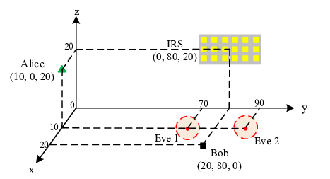
In this section, numerical results are provided to demonstrate the effectiveness of the proposed RSBF schemes. As shown in Fig. 2, it is assumed that Alice, IRS and Bob are respectively located at (10, 0, 20), (0, 80, 20) and (20, 80, 0) in meters. While two Eves (i.e., K=2K=2) are located within two circular regions, nearby (10, 70, 0) and (10, 90, 0) in meters, respectively. The large-scale fading βj{\beta_{j}} is taken as βj​(c,d)=ς0−10​c​log10⁡(dj){\beta_{j}}\left({c,d}\right)={\varsigma_{0}}-10c{\log_{10}}\left({{d_{j}}}\right) where djd_{j} denotes the signals propagation distance and the the path loss exponents of LoS and No-LoS are set as cL​o​S=2{c_{LoS}}\!=\!2 and cN​L​o​S=5{c_{NLoS}}\!=\!5, respectively. We set M=16M\!=\!16, N=Na​z×Ne​l=4×4N\!=\!N_{az}\times N_{el}\!=\!4\times 4, ε=10−3\varepsilon\!=\!{10^{-3}}, L=4L\!=\!4, ς0=−61.4​d​B{\varsigma_{0}}\!=\!-61.4~dB and σ02=−110​d​B​m\sigma_{0}^{2}\!=\!-110~dBm. The maximum ratio transmission (MRT)-based scheme, perfect CSI based scheme [8] and average based scheme are adopted for performance comparison, where MRT-based scheme means that the passive BF vector is optimized to maximize ‖𝐡R​B​𝐐𝐇A​R‖\left\|{{{\bf{h}}_{RB}}{\bf{Q}}{{\bf{H}}_{AR}}}\right\| and the active BF vector is designed based on MRT, while the average-based scheme means that the active and passive BF vectors are jointly optimized based on average of Eves’ AoAs.

Refer to caption
Fig. 3: ASR versus AoA error bound, Pm​a​x=1​WP_{max}=1~W.

Fig.3 depicts the ASR versus the AoA-based uncertainty of Eves for different BF algorithms, where the perfect CSI based scheme is provided as the upper bound. It can be observed that the ASR of the MRT-based scheme keeps stable as the error bound of AoA increases but is worse than others. This is due to the fact that the ASR of MRT-based scheme only depends on the CSI of legitimate channels. Meanwhile, the ASR of the proposed RSBF scheme decreases slowly as the error bound of AoA increases. In contrast, the ASR of the average-based scheme significantly decreases, which validates the robustness of proposed RSBF scheme.

Fig.4 plots the ASR versus the transmission power for different BF algorithms with both colluding and non-colluding eavesdropping scenarios. It can be observed that the gap between upper bound and the proposed RSBF scheme is smaller than that between upper bound and the MRT-based scheme, which demonstrates the effectiveness and superiority of the proposed RSBF scheme. Meanwhile, the ASR of perfect CSI scheme and proposed RSBF scheme significantly increase, but that of MRT-based scheme increases slowly and even keeps zero for the colluding eavesdropping scenario as the transmission power increases. This is due to the fact that the MRT-based scheme aims to maximize the achievable rate of Bob while ignoring Eves, which results in significant information leakage since the Eves are located nearby Bob, while the proposed RSBF scheme can effectively prevent eavesdropping against the imperfect CSI of Eves’ channels.

Refer to caption
Fig. 4: ASR versus transmission power, Δ=5∘\Delta=5^{\circ}.

VI Conclusion

In this letter, we have investigated an RSBF scheme in an IRS-aided mmWave secrecy system, against multiple single antenna Eves. Considering the AoA-based CSI of Eves’ channels is imperfectly known by the legitimate transmitter, we formulate optimization problems to maximize the worst case of ASR for both colluding and non-colluding eavesdropping scenarios, and propose a robust algorithm to solve such non-convex problems. Numerical results are provided to illustrate the effectiveness of proposed RSBF schemes.

References

  • [1] M. Xiao, S. Mumtaz, Y. Huang and L. Dai el., “Millimeter Wave Communications for Future Mobile Networks,” IEEE J. Sel. Areas Commun., vol. 35, no. 9, pp. 1909–1935, Sep. 2019.
  • [2] S. Zhang, Q. Wu, S. Xu and G. Li, “Fundamental Green Tradeoffs: Progresses, Challenges, and Impacts on 5G Networks,” IEEE Commun. Surveys Tuts., vol. 19, no. 1, pp. 33–56, First Quarter 2017.
  • [3] Q. Wu and R. Zhang, “Intelligent Reflecting Surface Enhanced Wireless Network via Joint Active and Passive Beamforming,” IEEE Trans. Wireless Commun., vol. 18, no. 11, pp. 5394–5409, Nov. 2019.
  • [4] Q. Wu and R. Zhang, “Towards Smart and Reconfigurable Environment: Intelligent Reflecting Surface Aided Wireless Network,” IEEE Commun. Mag., DOI:10.1109/MCOM.001.1900107.
  • [5] Q. Wu and R. Zhang, “Beamforming Optimization for Wireless Network Aided by Intelligent Reflecting Surface with Discrete Phase Shifts,” IEEE Trans. Commun., DOI: 10.1109/TCOMM.2019.2958916
  • [6] C. Huang et al., “Holographic MIMO Surfaces for 6G Wireless Networks: Opportunities, Challenges, and Trends,” [Online] Available: https://arxiv.org/abs/1911.12296.
  • [7] P. Cao, and T. Lv, “Intelligent Reflecting Surface Aided Multi-User Millimeter-Wave Communications for Coverage Enhancement,” [Online] Available: https://arxiv.org/abs/1910.02398.
  • [8] M. Cui, G. Zhang and R. Zhang, “Secure wireless communication via intelligent reflecting surface,” IEEE Wireless Commun. Lett., DOI: 10.1109/LWC.2019.2919685.
  • [9] S. Hong, C. Pan, H. Ren, K. Wang and A. Nallanathan, “Artificial-Noise-Aided Secure MIMO Wireless Communications via Intelligent Reflecting Surface,” [Online] Available: https://arxiv.org/abs/2002.07063.
  • [10] X. Guan, Q. Wu and R. Zhang, “Intelligent Reflecting Surface Assisted Secrecy Communication : Is Artificial Noise Helpful or Not?” IEEE Wireless Commun. Lett., Jan. 2020, DOI: 10.1109/LWC.2020.2969629.
  • [11] Z. He and X. Yuan, “Cascaded Channel Estimation for Large Intelligent Metasurface Assisted Massive MIMO,” [Online]. Available:https://arxiv.org/pdf/1905.07948.
  • [12] C. You, B. Zheng and R. Zhang, “Intelligent Reflecting Surface with Discrete Phase Shifts: Channel Estimation and Passive Beamforming,” [Online]. Available:https://arxiv.org/abs/1911.03916.
  • [13] J. Chen, Y.-C. Liang, H. Cheng and W. Yu, “Channel Estimation for Reconfigurable Intelligent Surface Aided Multi-User MIMO Systems,” [Online]. Available:https://arxiv.org/abs/1912.03619.
  • [14] Z. Lin, M. Lin, J. Wang, Y. Huang and W. Zhu, “Robust Secure Beamforming for 5G Cellular Networks Coexisting With Satellite Networks,” IEEE J. Sel. Areas Commun., vol. 36, no. 4, pp. 932–945, Apr. 2018.
  • [15] S. Boyd and L. Vandenberghe, “Convex Optimization, Cambridge,” U.K.: Cambridge Univ. Press, 2004.