Voltage distribution in a non-locally but globally electroneutral confined electrolyte medium: applications for nanophysiology

A. Tricot I.M. Sokolov

*

D. Holcman Note: $ˆ1$ Data Modeling, Computational Biology and Predictive Medicine, Ecole Normale Supérieure, 46 rue d’Ulm 75005 Paris, France.$ˆ2$ Institute of Physics and IRIS Adlershof, Humboldt University Berlin, Newtonstr. 15, 12489 Berlin, Germany.

Abstract

The distribution of voltage in sub-micron cellular domains remains poorly understood. In neurons, the voltage results from the difference in ionic concentrations which are continuously maintained by pumps and exchangers. However, it not clear how electro-neutrality could be maintained by an excess of fast moving positive ions that should be counter balanced by slow diffusing negatively charged proteins. Using the theory of electro-diffusion, we study here the voltage distribution in a generic domain, which consists of two concentric disks (resp. ball) in two (resp. three) dimensions, where a negative charge is fixed in the inner domain. When global but not local electro-neutrality is maintained, we solve the Poisson-Nernst-Planck equation both analytically and numerically in dimension 1 (flat) and 2 (cylindrical) and found that the voltage changes considerably on a spatial scale which is much larger than the Debye screening length, which assumes electro-neutrality. The present result suggests that long-range voltage drop changes are expected in neuronal microcompartments, probably relevant to explain the activation of far away voltage-gated channels located on the surface.

1 Introduction

How voltage and ionic concentrations are distributed and regulated in excitable cells such as neurons, astrocytes, etc.. remains a challenging question, despite decades of experimental and theoretical efforts [1, 2, 3, 4, 5, 6, 7]. In particular, the voltage in microdomains such as initial segments, dendrites, dendritic spines, remain difficult to study experimentally due to their small size. The ionic concentrations are constantly regulated in order to maintain the physiological gradients: while potassium ions are extruded, sodium ions must be pumped in through energy dependent exchangers [1]. In recent years, the voltage distribution and the ionic currents have been measured using nanopipettes [8, 9] and voltage dyes [10]. Neuronal microdomains are characterized by an excess of positive ions (sodium and potassium), not compensated by chloride. However the missing negative charges should be carried by heavy proteins and molecules inside the cytoplasm characterized by small diffusion coefficients compared to the ones of the main ions. Yet, the overall cytoplasmic medium is expected to be electroneutral, although measurements should be performed [10, 6] in cellular domains such as dendritic spines, pre-synaptic terminal or glial protrusions.
The classical framework to study electrical properties of cytoplasm which are electrolytes is the electro-diffusion theory [1, 11, 12] which consists of modeling the motion of diffusing ions in water, where the electrostatic force is due to the charge concentration differences between positive and negative species.
In the classical Debye theory [1], the voltage of a charge immersed is estimating in a neutral electrolyte. This theory predicts a screening of an excess charge, due to the exponential decay of the electrical field. The theory is based on two main assumptions 1) the field induced by the excess charge is small compared to thermal fluctuations and 2) a strict electroneutrality condition imposed at infinity, where the concentration of positive and the negative charges are equal far away of the immersion of the test volume. The Debye characteristic length is $\lambda_{D}=\left(\frac{\varepsilon\varepsilon_{0}k_{B}T}{z^{2}e^{2}N_{A}c_{0}}\right)^{\frac{1}{2}}$ , for the electron charge $e$ , The temperature $T$ , the Boltzmann constant $k_{B}$ , the valence $z$ , the vacuum permittivity $\varepsilon_{0}$ and $\varepsilon$ the relative permittivity of the ions, the avogadro number $N_{A}$ and the concentration of ions $c_{0}$ .
In the extreme case of non-electrical medium, theoretical analysis and numerical simulations revealed a long-range log-decay of the electric field [13, 14, 15, 16] and a modulation of the voltage distribution due to an oscillating [17] or a cusp [16, 18] geometry.
In this manuscript, we compute the voltage and charge distribution when the condition of global but not local electro-neutrality is maintained. We consider a ball containing positive and negative charges, however a fraction of negative charges is fixed in the inner ball (Fig. 1). The external boundary does not allow charges to escape. The manuscript is organized as follows: in section 1, we present general PNP model. We summarize our main results in table 1. In section 2, we treat the case of one dimension. We solve the PNP equation using elliptic integrals and obtain the decay of the voltage near the boundary. In section 3, we study the solutions in dimensions two and three. We determine the voltage and charge distribution when we vary the static negative charges.

2 Model of global but not local electroneutrality

To model global but not local electro-neutrality, we use an elementary geometry of a domain $\Omega$ consisting in two concentric disks in dimension two and balls in dimension three. We impose a negative charge inside (Fig. 1).

Figure 1: Schematic representation of the geometry

\Omega

made of two concentric disks: the small one

\Omega_{0}

containing the fixed charged

Q^{-}=-Nze

, modeling impenetrable proteins (red circle). Between the red boundary and the blue one, negative charges (total charge

q^{-}=-n^{-}ze

, that could represent chloride ions) is mixed in water with positive ions

q^{+}=n^{+}ze

, representing potassium and sodium. The global electro-neutrality imposes

Q^{-}+q^{-}+q^{+}=0

(equivalently

N+n^{-}=n^{+}

2.1 The Poisson-Nernst-Planck equations in the domain $\Omega$

The coarse-grain Poisson-Nernst-Planck equations model electro-diffusion [1, 19, 12] in a electrolyte. In the domain $\Omega$ (Fig. 1), the total charge is the sum of mobile positive $n^{+}$ and negative $n^{-}$ charges plus a fixed number negative charges $N^{static}=N$ located in an impenetrable (unaccessible) subregion $\Omega_{0}\subset\Omega$ (red circle in Fig. 1), representing negatively charged proteins. We assume global electroneutrality:

\displaystyle N+n^{-}=n^{+}.

(1)

For a ionic valence $z$ , the total number of particles is

\displaystyle\int\limits_{\Omega-\Omega_{0}}\rho_{p}(\tilde{\mbox{\boldmath$x$}},t)d\tilde{\mbox{\boldmath$x$}}=n^{+},\,\int\limits_{\Omega-\Omega_{0}}\rho_{n}(\tilde{\mbox{\boldmath$x$}},t)d\tilde{\mbox{\boldmath$x$}}=n^{-}

(2)

and thus the total charge is

\displaystyle q_{\pm}=\pm zeN,\,Q^{-}+q^{-}+q^{+}=0

where $e$ is the electron charge. The particle density $\rho_{p}(\tilde{\mbox{\boldmath$x$}},t)$ is the solution of the Nernst-Planck equation

$\displaystyle D\left[\Delta\rho_{p}(\tilde{\mbox{\boldmath$x$}},t)+\frac{ze}{kT}\nabla\cdot\left(\rho_{p}(\tilde{\mbox{\boldmath$x$}},t)\nabla\phi(\tilde{\mbox{\boldmath$x$}},t)\right)\right]$	$\displaystyle=$	$\displaystyle\,\frac{\partial\rho_{p}(\tilde{\mbox{\boldmath$x$}},t)}{\partial t}\hskip 5.0pt\mbox{for}\ \tilde{\mbox{\boldmath$x$}}\in\Omega-\Omega_{0}$
$\displaystyle D\left[\Delta\rho_{n}(\tilde{\mbox{\boldmath$x$}},t)-\frac{ze}{kT}\nabla\cdot\left(\rho_{n}(\tilde{\mbox{\boldmath$x$}},t)\nabla\phi(\tilde{\mbox{\boldmath$x$}},t)\right)\right]$	$\displaystyle=$	$\displaystyle\,\frac{\partial\rho_{n}(\tilde{\mbox{\boldmath$x$}},t)}{\partial t}\hskip 5.0pt\mbox{for}\ \tilde{\mbox{\boldmath$x$}}\in\Omega-\Omega_{0}$
$\displaystyle D\left[\frac{\partial\rho(\tilde{\mbox{\boldmath$x$}},t)}{\partial n}+\frac{ze}{kT}\rho(\tilde{\mbox{\boldmath$x$}},t)\frac{\partial\phi(\tilde{\mbox{\boldmath$x$}},t)}{\partial n}\right]$	$\displaystyle=$	$\displaystyle\,0\hskip 5.0pt\mbox{for}\ \tilde{\mbox{\boldmath$x$}}\in\partial\Omega-\partial\Omega_{0}$	(3)
$\displaystyle\rho(\tilde{\mbox{\boldmath$x$}},0)$	$\displaystyle=$	$\displaystyle\,{\rho_{0}}(\tilde{\mbox{\boldmath$x$}})\hskip 5.0pt\mbox{for}\ \tilde{\mbox{\boldmath$x$}}\in\tilde{\Omega},$	(4)

where $kT$ represents the thermal energy. The electric potential $\phi(\tilde{\mbox{\boldmath$x$}},t)$ in $\tilde{\Omega}$ satisfies the Poisson equation

	$\displaystyle\Delta\phi(\tilde{\mbox{\boldmath$x$}},t)=$	$\displaystyle\,-\frac{ze\left(\rho_{p}(\tilde{\mbox{\boldmath$x$}},t)-\rho_{n}(\tilde{\mbox{\boldmath$x$}},t)\right)}{\varepsilon_{r}\varepsilon_{0}}\hskip 5.0pt\mbox{for}\ \tilde{\mbox{\boldmath$x$}}\in\tilde{\Omega}$		(5)
	$\displaystyle\frac{\partial\phi(\tilde{\mbox{\boldmath$x$}},t)}{\partial n}=$	$\displaystyle\,-\tilde{\sigma}(\tilde{\mbox{\boldmath$x$}},t)\hskip 5.0pt\mbox{for}\ \tilde{\mbox{\boldmath$x$}}\in{\partial\Omega-\Omega_{0}},$		(6)

where $\varepsilon_{r}\varepsilon_{0}$ is the permittivity of the medium and $\tilde{\sigma}(\tilde{\mbox{\boldmath$x$}},t)$ is the surface charge density on the boundary $\partial\Omega$ .

2.2 Steady-state solution

To study the effect of non-local electroneutrality, we study the solution of the steady-state equation (2.1) in the normalized domain $\tilde{\Omega}$ (of radius 1). The Boltzmann distributions are given by

	$\displaystyle\rho_{p}(\tilde{\mbox{\boldmath$x$}})=n^{+}\frac{\exp\left\{-\displaystyle\frac{ze\phi(\tilde{\mbox{\boldmath$x$}})}{kT}\right\}}{\int_{\tilde{\Omega}-\tilde{\Omega}_{0}}\exp\left\{-\displaystyle\frac{ze\phi(\mbox{\boldmath$x$})}{kT}\right\}\,d\mbox{\boldmath$x$}},$		(7)
	$\displaystyle\rho_{n}(\tilde{\mbox{\boldmath$x$}})=n^{-}\frac{\exp\left\{\displaystyle\frac{ze\phi(\tilde{\mbox{\boldmath$x$}})}{kT}\right\}}{\int_{\tilde{\Omega}-\tilde{\Omega}_{0}}\exp\left\{\displaystyle\frac{ze\phi(\mbox{\boldmath$x$})}{kT}\right\}\,d\mbox{\boldmath$x$}},$		(8)

hence (5) results in the nonlinear Poisson equation

\displaystyle\Delta\phi(\tilde{\mbox{\boldmath$x$}})=-\frac{zeN_{p}\exp\left\{-\displaystyle\frac{ze\phi(\tilde{\mbox{\boldmath$x$}})}{kT}\right\}}{\varepsilon_{r}\varepsilon_{0}{\displaystyle\int_{\tilde{\Omega}-\tilde{\Omega}_{0}}\exp\left\{-\displaystyle\frac{ze\phi(\mbox{\boldmath$s$})}{kT}\right\}\,d\mbox{\boldmath$s$}}}+\frac{zeN_{n}\exp\left\{\displaystyle\frac{ze\phi(\tilde{\mbox{\boldmath$x$}})}{kT}\right\}}{\varepsilon_{r}\varepsilon_{0}{\displaystyle\int_{\tilde{\Omega}-\tilde{\Omega}_{0}}\exp\left\{\displaystyle\frac{ze\phi(\mbox{\boldmath$s$})}{kT}\right\}\,d\mbox{\boldmath$s$}}}.

(9)

In region $\tilde{\Omega}_{1}$ , the Poisson equation is

\displaystyle\Delta\phi(\tilde{\mbox{\boldmath$x$}})=-\frac{zeN}{\varepsilon_{r}\varepsilon_{0}V_{1}},

(10)

and thus

\displaystyle\int_{\Sigma_{0}}\frac{\partial\phi({\tilde{\mbox{\boldmath$x$}}})}{\partial n}dS_{\mbox{\boldmath$x$}}=-\frac{zeN}{\varepsilon_{r}\varepsilon_{0}},

(11)

where $\Sigma_{0}$ is the boundary of $\Omega_{0}$ . The global electro-neutrality (relation 1) leads to the compatibility condition imposed by Gauss flux integral

\displaystyle\int_{\Sigma_{0}}\frac{\partial\phi({\tilde{\mbox{\boldmath$x$}}})}{\partial n}dS_{\mbox{\boldmath$x$}}-\int_{\Sigma}\frac{\partial\phi({\tilde{\mbox{\boldmath$x$}}})}{\partial n}dS_{\mbox{\boldmath$x$}}=n^{+}-n^{-}.

(12)

Thus,

\displaystyle\int_{\Sigma}\frac{\partial\phi({\tilde{\mbox{\boldmath$x$}}})}{\partial n}dS_{\mbox{\boldmath$x$}}=0.

(13)

By symmetry, we impose that $\displaystyle\frac{\partial\phi}{\partial n}$ is constant on the two surfaces $\Sigma$ and $\Sigma_{0}$ and thus we impose the conditions:

	$\displaystyle\frac{\partial\phi({\tilde{\mbox{\boldmath$x$}}})}{\partial n}$	$\displaystyle=$	$\displaystyle-\frac{zeN}{\varepsilon_{r}\varepsilon_{0}\|\Sigma_{1}\|}\,\mbox{ for }\,\tilde{\mbox{\boldmath$x$}}\in\Sigma_{0}.$		(14)
	$\displaystyle\frac{\partial\phi({\tilde{\mbox{\boldmath$x$}}})}{\partial n}$	$\displaystyle=$	$\displaystyle 0\,\mbox{ for }\,\tilde{\mbox{\boldmath$x$}}\in\Sigma.$		(15)

In spherical symmetry, the Poisson’s equation (9) reduces to

	$\displaystyle\Phi^{\prime\prime}(r)+\frac{d-1}{r}\Phi^{\prime}(r)=\frac{ze}{\varepsilon\varepsilon_{0}S_{d}}$	$\displaystyle\left(n^{-}\frac{\displaystyle\exp\left(\frac{\displaystyle ze\Phi(r)}{\displaystyle k_{B}T}\right)}{\displaystyle\int_{R_{0}}^{R}\exp\left(\frac{\displaystyle ze\Phi(r)}{\displaystyle k_{B}T}\right)r^{d-1}dr}\right.$			(16)
		$\displaystyle-\left.n^{+}\frac{\displaystyle\exp\left(-\frac{\displaystyle ze\Phi(r)}{\displaystyle k_{B}T}\right)}{\displaystyle\int_{R_{0}}^{R}\exp\left(-\frac{\displaystyle ze\Phi(r)}{\displaystyle k_{B}T}\right)r^{d-1}dr}\right).$			(17)

We normalize the radius by setting $r=Rx$ for $a\leq x\leq 1$ where $a=\frac{R_{0}}{R}$ . Here

\displaystyle u=\frac{ze}{k_{B}T}\Phi,\quad\lambda_{d}=\frac{(ze)^{2}}{S_{d}R^{d-2}\varepsilon\varepsilon_{0}k_{B}T}

(18)

Here $S_{d}$ is the surface area of the unit sphere in $\mathbb{R}^{d}$ . Eq.(16) becomes

\displaystyle u^{\prime\prime}(x)+\frac{d-1}{x}u^{\prime}(x)=I_{\lambda}e^{u(x)}-J_{\lambda}e^{-u(x)},

(19)

where we use the notations

\displaystyle I_{\lambda}=\frac{\displaystyle n^{-}\lambda_{d}}{\displaystyle\int_{a}^{1}\exp\left(\frac{\displaystyle ze\Phi(x)}{\displaystyle k_{B}T}\right)x^{d-1}dx},\quad J_{\lambda}=\frac{\displaystyle n^{+}\lambda_{d}}{\displaystyle\int_{a}^{1}\exp\left(-\frac{\displaystyle ze\Phi(x)}{\displaystyle k_{B}T}\right)x^{d-1}dx}.

(20)

We shall study the anionic $I_{\lambda}$ and cationic $J_{\lambda}$ strengths vs $\lambda$ and the solution $u$ . Our goal here is to determine $u$ over the ball $\tilde{\Omega}$ . The condition $u^{\prime}(1)=0$ is satisfied due to the global electro-neutrality. We impose that the voltage is zero on $\Sigma$ , as it is defined to an additive constant. In summary the boundary conditions are

\displaystyle u(1)=0,\quad u^{\prime}(1)=0.

(21)

Eq.(19) and the boundary conditions in eq.(21) together form a one dimensional boundary value problem with the following properties:

•

the derivative $u^{\prime}$ is maximal at point $a$ and decreases toward $u^{\prime}(1)=0$ .
•

$u$ is minimal at $x=a$ and increases toward $u(1)=0$ .
•

$u^{\prime\prime}(1)=I_{\lambda}-J_{\lambda}\leq 0$ i.e. $J_{\lambda}\geq I_{\lambda}$ .

The strategy to find the solution is the following: since the parameters $I_{\lambda}$ and $J_{\lambda}$ depend on the solution $u$ , we will first search for an analytical solution for any value of the parameter $\lambda$ . We will then self-consistently compute the expression of $I_{\lambda}$ and $J_{\lambda}$ . This steps imposes some restriction and we will show that solutions exist only for specific values of $(I_{\lambda},J_{\lambda})$ .

3 steady-state Solution of PNP eq.(19) in flat geometry (dimension 1)

Refer to caption — Figure 2: Normalized potential $u(r)$ in dimension 1 for $\tilde{\Omega}=[0,1]$ . A. Schematic representation of the domain. B. Allowed (red) and forbidden regions for the parameters $I_{\lambda}$ and $J_{\lambda}$ . The squares, crosses and triangles respectively refer to the curves on panels C, D and E. C. Solution $u(r)$ with constant cationic strength $J_{\lambda}$ and increasing anionic strength $I_{\lambda}$ . By increasing $I_{\lambda}$ , the amplitude of the solution decays. D. No negative ions in the region $[0,a]$ . The critical solution (dashed) develops a singularity in $r=a$ .E. Critical solutions with a singularity at $r=a$ . The parameters $I_{\lambda}$ and $J_{\lambda}$ are on the boundary of the red domain satifying relation $\sqrt{I_{\lambda}}+\sqrt{J_{\lambda}}=\frac{\sqrt{2}K(k)}{1-a}$ .

In dimension 1, the normalized domain $\tilde{\Omega}$ is the interval $\tilde{\Omega}=[0,1]$ (Fig. 2A). The fixed negative charges are located in $[0,a]$ while the mobile ions are in $a<x<1$ . The boundary value problem eq.(19) reduces to

	$\displaystyle u^{\prime\prime}(x)$	$\displaystyle=$	$\displaystyle I_{\lambda}e^{u(x)}-J_{\lambda}e^{-u(x)}\qquad\text{for $a<x<1$},$		(22)
	$\displaystyle u(1)$	$\displaystyle=$	$\displaystyle 0,\quad u^{\prime}(1)=0.$

We show by direct integration in Appendices 7.1 and 7.2 that the general solution can be expressed in terms of the Jacobian elliptic functions [20]

\displaystyle u(x)=-2\ln\left(\frac{1}{2}\frac{\sqrt{I_{\lambda}}+\sqrt{J_{\lambda}}}{\sqrt{J_{\lambda}}}\left(\operatorname{dc}\left(\frac{\sqrt{I_{\lambda}}+\sqrt{J_{\lambda}}}{\sqrt{2}}(x-1)\right)+\sqrt{1-k_{\lambda}^{2}}\operatorname{nc}\left(\frac{\sqrt{I_{\lambda}}+\sqrt{J_{\lambda}}}{\sqrt{2}}(x-1)\right)\right)\right),

(23)

where $\operatorname{dc}$ and $\operatorname{nc}$ are the elliptic functions [20] of modulus

\displaystyle k_{\lambda}=\sqrt{\frac{2}{1-c}}=\frac{\displaystyle 2\sqrt[4]{I_{\lambda}J_{\lambda}}}{\displaystyle\sqrt{I_{\lambda}}+\sqrt{J_{\lambda}}},

(24)

with $0<k\leq 1$ . The parameters $I_{\lambda}$ and $J_{\lambda}$ satisfy the inequality (Appendix 7.1)

\displaystyle\sqrt{I_{\lambda}}+\sqrt{J_{\lambda}}\leq\frac{\sqrt{2}K(k)}{1-a},

(25)

where $K(k)$ is the complete elliptic integral of the first kind (Appendix 7.1). The possible region (red in Fig. 2B) is obtained by combining conditions 24 and 25. We plotted the solutions for various positive and negative charges (Fig. 2C-E). In the boundary of validity (eq.(25)), the solution $u$ develops a log-singularity at $x=a$ (Fig. 2 D-E, dashed lines). This situation is similar to the case of a single charge in the entire ball [15, 16]. It is interesting to observe the long -range voltage changes in this non-local electro-neutral medium, even in the limit of $a$ small (size of the impenetrable region containing negative charges). To obtain a closed form of the solution, we compute $I_{\lambda}$ and $J_{\lambda}$ (relation 20) with respect to the parameters $\lambda_{d}n^{+}$ , $\lambda_{d}n^{-}$ and $a$ . A direct integration of the function $e^{u(x)}$ and $e^{-u(x)}$ over the interval $[a,1]$ (In appendix 7.3) gives with

\displaystyle u_{a}=\frac{\sqrt{I_{\lambda}}+\sqrt{J_{\lambda}}}{\sqrt{2}}(a-1)

(26)

that

	$\displaystyle\displaystyle\lambda_{d}n^{-}$	$\displaystyle=\frac{\sqrt{I_{\lambda}}+\sqrt{J_{\lambda}}}{2\sqrt{2}}\left(f_{k_{\lambda}}(u_{a})+\frac{\sqrt{J_{\lambda}}-\sqrt{I_{\lambda}}}{\sqrt{I_{\lambda}}+\sqrt{J_{\lambda}}}g(u_{a})\right),$			(27)
	$\displaystyle\displaystyle\lambda_{d}n^{+}$	$\displaystyle=\frac{\sqrt{I_{\lambda}}+\sqrt{J_{\lambda}}}{2\sqrt{2}}\left(f_{k_{\lambda}}(u_{a})-\frac{\sqrt{J_{\lambda}}-\sqrt{I_{\lambda}}}{\sqrt{I_{\lambda}}+\sqrt{J_{\lambda}}}g(u_{a})\right),$			(28)

where we defined the two functions (Fig. 3)

	$\displaystyle f_{k}(x)$	$\displaystyle=$	$\displaystyle 2\operatorname{E}(x)-(2-k^{2})x-2\operatorname{sn}(x)\operatorname{dc}(x),$		(29)
	$\displaystyle g(x)$	$\displaystyle=$	$\displaystyle 2\operatorname{sc}(x),\hbox{ for }x\in]-K(k);K(k)[.$		(30)

Note that we can write (from relation 24)

\displaystyle 1-k_{\lambda}^{2}=(\frac{\sqrt{J_{\lambda}}-\sqrt{I_{\lambda}}}{\sqrt{I_{\lambda}}+\sqrt{J_{\lambda}}})^{2}.

(31)

The parameter $k_{\lambda}$ represents the balance between the negative charges. Indeed,

•

$k_{\lambda}\longrightarrow 1$ , $I_{\lambda}\approx J_{\lambda}$ and eq.(32) implies $N\longrightarrow 0$ .
•

$k_{\lambda}\longrightarrow 0$ , $J_{\lambda}\gg I_{\lambda}$ . Using $I_{\lambda}$ in eq.(20), we get $n^{-}\longrightarrow 0$ .

Finally, the global electro-neutrality condition leads to the relation

\displaystyle\lambda_{d}N=-\frac{\sqrt{J_{\lambda}}-\sqrt{I_{\lambda}}}{\sqrt{2}}g(u_{a}).

(32)

To conclude, for each positive and negative density ( $n^{+},n^{-}$ ) satisfying electroneutrality 1, the system of equations 27-28-31-32 can be resolved and there is a unique couple ( $J_{\lambda},I_{\lambda}$ ) for which condition (25) is satisfied, and thus the solution $u(x)$ is defined on the entire interval $[a,1]$ .

3.1 Explicit expressions for the difference of potential $u(1)-u(a)$

We study here the potential difference between the surfaces of the two balls.

\displaystyle u(1)-u(a)=2\ln\left(\frac{1}{2}\frac{\sqrt{I_{\lambda}}+\sqrt{J_{\lambda}}}{\sqrt{J_{\lambda}}}\left(\operatorname{dc}(u_{a})+\sqrt{1-k_{\lambda}^{2}}\operatorname{nc}(u_{a})\right)\right),

(33)

where

\displaystyle u_{a}=\frac{\sqrt{I_{\lambda}}+\sqrt{J_{\lambda}}}{\sqrt{2}}(a-1).

(34)

The potential difference $u(1)-u(a)$ has a minimum when $I_{\lambda}=J_{\lambda}$ and grows with the difference between $I_{\lambda}$ and $J_{\lambda}$ . The limit value for this difference depends on the value of the sum $\sqrt{I_{\lambda}}+\sqrt{J_{\lambda}}$ as shown by eq.(25). We shall now study some limit cases for the potential difference $u(1)-u(a)$ .

3.1.1 Case $n^{-}\longrightarrow 0$ ( $n^{+}=N$ )

In the case $n^{-}=0$ , we have $I_{\lambda}=0$ (eq.(20)) and $k_{\lambda}=0$ . From eq.(28), we obtain

\displaystyle\lambda_{d}n^{+}=\frac{\sqrt{J_{\lambda}}}{2\sqrt{2}}\left(f(u_{a})-g(u_{a})\right).

(35)

When $k=0$ , the Jacobian elliptic functions simplifies to trigonometric functions

\displaystyle f(u_{a})=-2\tan(u_{a}),g(u_{a})=2\tan(u_{a}),

(36)

with $u_{a}=\sqrt{\frac{J_{\lambda}}{2}}(a-1)$ , eq.(35) becomes

\displaystyle\lambda_{d}n^{+}=\sqrt{2J_{\lambda}}\tan\left(\frac{\sqrt{2J_{\lambda}}}{2}(1-a)\right).

(37)

We recover the asymptotic result [21] for positive ions in a ball. The solutions for $n^{+}\geq 0$ leads to $0\leq J_{\lambda}\leq\frac{\pi^{2}}{2(1-a)^{2}}$ . The potential difference is

\displaystyle u(1)-u(a)=-2\ln\left(2\cos\left(\sqrt{\frac{J_{\lambda}}{2}}(1-a)\right)\right),

(38)

where $J_{\lambda}$ is the solution of eq.(37) for a given $n^{+}$ .

3.1.2 Case $N=0$ ( $n^{+}=n^{-}$ )

In the case $N=0$ , eq.(32) implies $I_{\lambda}=J_{\lambda}$ and thus $k_{\lambda}=1$ . Eq.(28) becomes

\displaystyle\lambda_{d}n^{+}=\sqrt{\frac{J_{\lambda}}{2}}f(u_{a}).

(39)

When $k_{\lambda}=1$ , Jacobian elliptic functions simplify to hyperbolic functions, which gives $E(u)=\tanh(u)\ ,\quad\operatorname{sn}(u)=\tanh(u)\ ,\quad\operatorname{cn}(u)=\operatorname{dn}(u)=\frac{1}{\cosh(u)},$ and $f(u_{a})=2\tanh(u_{a})-u_{a}-2\tanh(u_{a})=-u_{a}$ . Eq.(39) becomes

\displaystyle J_{\lambda}=\frac{\lambda_{d}n^{+}}{1-a},

(40)

the Jacobian function $\operatorname{dc}=1$ , and thus $u(r)=0$ for $r\in[a,1]$ . The behavior of $u$ for small $N$ is shown in fig. 4 with $J_{\lambda}=1.01I_{\lambda}$ .

Expanding the Jacobian elliptic functions for $k$ near $1$ , we obtain

	$\displaystyle\operatorname{dc}(u)$	$\displaystyle=1+\frac{1}{2}(1-k^{2})\sinh^{2}(u)+\circ(1-k^{2}),$			(41)
	$\displaystyle\operatorname{nc}(u)$	$\displaystyle=\cosh(u)+\circ(1-k^{2}),$			(42)

and thus

\displaystyle u(1)-u(a)

\displaystyle=2\ln\left(\frac{1}{2}\frac{\sqrt{I_{\lambda}}+\sqrt{J_{\lambda}}}{\sqrt{J_{\lambda}}}\left(1+\frac{1}{2}(1-k^{2})\sinh^{2}(u_{a})+\sqrt{1-k^{2}}\cosh(u_{a})\right)\right)

Since $k\longrightarrow 1$ , we finally obtain

\displaystyle u(1)-u(a)\sim\frac{\sqrt{J_{\lambda}}-\sqrt{I_{\lambda}}}{\sqrt{J_{\lambda}}}\left(\frac{1}{2}\frac{\sqrt{J_{\lambda}}-\sqrt{I_{\lambda}}}{\sqrt{J_{\lambda}}+\sqrt{I_{\lambda}}}\sinh^{2}(u_{a})+\cosh(u_{a})-1\right).

(43)

3.1.3 Case $u_{a}\ll 1$

For $u_{a}\ll 1$ we can obtain from Appendix 7.2 (expression of $f$ and $g$ in eq.(29))

	$\displaystyle f(u_{a})\sim(k^{2}-2)u_{a}=\frac{2}{\sqrt{2}}\frac{I_{\lambda}+J_{\lambda}}{\sqrt{I_{\lambda}}+\sqrt{J_{\lambda}}}(1-a),$		(44)
	$\displaystyle g(u_{a})\sim 2u_{a}=-\frac{2}{\sqrt{2}}\left(\sqrt{I_{\lambda}}+\sqrt{J_{\lambda}}\right)(1-a),$		(45)

so eq.(28) gives

\displaystyle\frac{\lambda_{d}n^{-}}{1-a}

\displaystyle=\frac{1}{2}\left(I_{\lambda}+J_{\lambda}-\left(J_{\lambda}-I_{\lambda}\right)\right),\hbox{ and }\frac{\lambda_{d}n^{+}}{1-a}

\displaystyle=\frac{1}{2}\left(I_{\lambda}+J_{\lambda}+J_{\lambda}-I_{\lambda}\right).

(46)

For $u_{a}\ll 1$ ,

\displaystyle\frac{\lambda_{d}n^{-}}{1-a}

\displaystyle=I_{\lambda}\hbox{ and }\frac{\lambda_{d}n^{+}}{1-a}

\displaystyle=J_{\lambda}.

(47)

Since $u_{a}=\frac{\sqrt{I_{\lambda}}+\sqrt{J_{\lambda}}}{\sqrt{2}}(a-1)$ , equations eq.(47) corresponds to few ions. To compute potential difference , we expand the Jacobian elliptic functions $\operatorname{dc}$ and $\operatorname{nc}$ for $u\ll 1$ :

\displaystyle\operatorname{dc}(u)

\displaystyle=1+(1-k^{2})\frac{u^{2}}{2}+\circ(u^{2}),\,\operatorname{nc}(u)

\displaystyle=1+\frac{u^{2}}{2}+\circ(u^{2}),

(48)

which gives

	$\displaystyle\operatorname{dc}(u_{a})+\sqrt{1-k^{2}}\operatorname{nc}(u_{a})$	$\displaystyle=1+\sqrt{1-k^{2}}+\frac{1}{2}\left(1-k^{2}+\sqrt{1-k^{2}}\right)u^{2}+\circ(u^{2})$			(49)
		$\displaystyle\sim\frac{2\sqrt{J_{\lambda}}}{\sqrt{I_{\lambda}}+\sqrt{J_{\lambda}}}+\frac{1}{2}\sqrt{J_{\lambda}}\left(\sqrt{J_{\lambda}}-\sqrt{I_{\lambda}}\right)(1-a)^{2}$			(49)

and thus

\displaystyle u(1)-u(a)\sim 2\ln\left(1+\frac{1}{4}\left(J_{\lambda}-I_{\lambda}\right)(1-a)^{2}\right)\sim\frac{1}{2}\lambda_{d}N(1-a).

(50)

3.1.4 Case $u_{a}\longrightarrow-K(k)$

When $u_{a}\longrightarrow-K(k)$ , we expand with respect to $u_{a}+K(k)$ the functions $f$ and $g$ using relation eq.(29):

	$\displaystyle f(u_{a})$	$\displaystyle=-2E(K(k))+\left(2-k^{2}\right)K(k)+\frac{2}{u_{a}+K(k)},$			(51)
	$\displaystyle g(u_{a})$	$\displaystyle=-\frac{2}{\sqrt{1-k^{2}}(u_{a}+K(k))}.$			(52)

From eq.(28), we get

	$\displaystyle\lambda_{d}n^{-}$	$\displaystyle=$	$\displaystyle\frac{\sqrt{I_{\lambda}}+\sqrt{J_{\lambda}}}{2\sqrt{2}}\left(-2E(K(k))+\left(2-k^{2}\right)K(k)\right),$		(53)
	$\displaystyle\lambda_{d}n^{+}$	$\displaystyle=$	$\displaystyle\frac{\sqrt{I_{\lambda}}+\sqrt{J_{\lambda}}}{2\sqrt{2}}\left(-2E(K(k))+\left(2-k^{2}\right)K(k)+\frac{4}{u_{a}+K(k)}\right),$		(54)

thus $n^{+}\longrightarrow\infty$ . Using

\displaystyle\lambda_{d}(n^{+}-n^{-})=\lambda_{d}N=\frac{\sqrt{I_{\lambda}}+\sqrt{J_{\lambda}}}{2\sqrt{2}}\frac{4}{u_{a}+K(k)},

(55)

we obtain that $N\longrightarrow\infty$ . Note that for $k=0$ , $E(K(0))=K(0)=\frac{\pi}{2}$ so $n^{-}=0$ . However, when $k\longrightarrow 1$ , $K(k)\longrightarrow\infty$ , then $n^{-}\longrightarrow\infty$ . The singularity is located at $r=a-\varepsilon$ with $\varepsilon\ll 1$ . Since $u_{a}=\frac{\sqrt{I_{\lambda}}+\sqrt{J_{\lambda}}}{\sqrt{2}}(a-1)$ , we have

\displaystyle u_{a-\varepsilon}=\frac{\sqrt{I_{\lambda}}+\sqrt{J_{\lambda}}}{\sqrt{2}}(a-\varepsilon-1)=-K(k)

(56)

and

\displaystyle u_{a}=-K(k)+\frac{\sqrt{I_{\lambda}}+\sqrt{J_{\lambda}}}{\sqrt{2}}\varepsilon.

(57)

Expanding the Jacobian elliptic functions $\operatorname{nc}$ and $\operatorname{dc}$ near $-K(k)$ :

\displaystyle\operatorname{dc}(u)\sim\frac{1}{u+K(k)},\qquad\operatorname{nc}(u)\sim\frac{1}{\sqrt{1-k^{2}}(u+K(k))},

(58)

using eq.(33) and eq.(57),we obtain

\displaystyle u(1)-u(a)=2\ln\left(\sqrt{\frac{2}{J_{\lambda}}}\frac{1}{\varepsilon}\right).

(59)

From the expression of $u_{a}+K(k)$ in eq.(57) and the formula for $\lambda_{d}N$ in eq.(55), we get $\lambda_{d}N=\frac{2}{\varepsilon}$ and finally

\displaystyle u(1)-u(a)=2\ln\left(\frac{\lambda_{d}N}{\sqrt{2J_{\lambda}}}\right).

(60)

When $n^{-}=0$ , similar to section 3.1.1, we get

\displaystyle\lambda_{d}n^{+}=\sqrt{2J_{\lambda}}\tan\left(\frac{\sqrt{2J_{\lambda}}}{2}(1-a)\right)

(61)

and since $n^{+}\longrightarrow\infty$ , $\sqrt{2J_{\lambda}}\longrightarrow\frac{\pi}{1-a}$ , we finally get

\displaystyle u(1)-u(a)\sim 2\ln\left(\frac{(1-a)\lambda_{d}N}{\pi}\right).

(62)

If $n^{-}\longrightarrow\infty$ , from eq.(53) $K(k)\longrightarrow\infty$ , which means that $k\longrightarrow 1$ and thus $J_{\lambda}-I_{\lambda}\longrightarrow 0$ . We can make the approximation

\displaystyle\sqrt{I_{\lambda}}+\sqrt{J_{\lambda}}\approx 2\sqrt{J_{\lambda}}

(63)

and write

\displaystyle\lambda_{d}n^{-}

\displaystyle=\frac{\sqrt{I_{\lambda}}+\sqrt{J_{\lambda}}}{2\sqrt{2}}\left(-2E(K(k))+\left(2-k^{2}\right)K(k)\right)

\displaystyle\sim\frac{\sqrt{I_{\lambda}}+\sqrt{J_{\lambda}}}{2\sqrt{2}}K(k)\sim J_{\lambda}(1-a)

Then using the expression of the potential difference in eq.(60), we obtain

\displaystyle u(1)-u(a)\sim 2\ln\left(\sqrt{\lambda_{d}(1-a)}\frac{N}{\sqrt{n^{-}}}\right).

(64)

In particular, when $n^{-}=N$ , we get

\displaystyle u(1)-u(a)\sim\ln\left(\lambda_{d}N(1-a)\right).

(65)

We have also plotted the function normalized potential $u(r)$ in Fig. 4-Right.

3.2 Summary potential difference $u(1)-u(a)$

We summarize in the table 1 below the differences of potential $u(1)-u(a)$ for the explicit solution in dimension 1, depending on the different condition on the mobile positive $n^{+}$ and negative $n^{-}$ charges satisfying the global electro-neutrality conditions $N+n^{-}=n^{+}$ .

Conditions	$u(1)-u(a)$
$\begin{matrix}n^{-}\longrightarrow 0(n^{+}=N)\\ \lambda_{d}n^{+}=\sqrt{2J_{\lambda}}\tan\left(\frac{\sqrt{2J_{\lambda}}}{2}(1-a)\right)\\ \end{matrix}$	$\displaystyle-2\ln\left(2\cos\left(\sqrt{\frac{J_{\lambda}}{2}}(1-a)\right)\right)$
$\begin{matrix}N=0(n^{+}\sim n^{-})\\ I_{\lambda}=J_{\lambda}\\ J_{\lambda}=\frac{\lambda_{d}n^{+}}{1-a}\\ u_{a}=\sqrt{2I_{\lambda}}(a-1)\\ \end{matrix}$	$\displaystyle\frac{\sqrt{J_{\lambda}}-\sqrt{I_{\lambda}}}{\sqrt{J_{\lambda}}}\left(\frac{1}{2}\frac{\sqrt{J_{\lambda}}-\sqrt{I_{\lambda}}}{\sqrt{J_{\lambda}}+\sqrt{I_{\lambda}}}\sinh^{2}(u_{a})+\cosh(u_{a})-1\right).$
$\begin{matrix}\frac{\sqrt{I_{\lambda}}+\sqrt{J_{\lambda}}}{\sqrt{2}}(a-1)\ll 1\\ \frac{\lambda_{d}n^{-}}{1-a}=I_{\lambda}\\ \frac{\lambda_{d}n^{+}}{1-a}=J_{\lambda}\end{matrix}$	$\displaystyle 2\ln\left(1+\frac{1}{4}\left(J_{\lambda}-I_{\lambda}\right)(1-a)^{2}\right)\sim\frac{1}{2}\lambda_{d}N(1-a)$
$\begin{matrix}N,n^{-},n^{+}\gg 1\\ \end{matrix}$	$\displaystyle 2\ln\left(\sqrt{\lambda_{d}(1-a)}\frac{N}{\sqrt{n^{-}}}\right).$
$\begin{matrix}N,n^{+}\gg 1\\ n^{-}=0\\ \end{matrix}$	$\displaystyle 2\ln\left(\frac{(1-a)\lambda_{d}N}{\pi}\right).$

Table 1: Electrodiffusion relations for the potential difference.

Finally, in fig. 5 we show the distribution of positive (red) and negative (blue) charge density computed in dimension 1 inside $[a,1]$ , associated to $u(a)-u(1)=7.207$ and $\lambda_{d}N=0.0887$ . Note that the difference of charge persists deep inside the domain.

4 Steady-solution in two dimensions

In this section, we resolve the PNP equation 19 in two dimensions (Fig. 6A), which reduces to

\displaystyle u^{\prime\prime}(r)+\frac{1}{r}u^{\prime}(r)=I_{\lambda}e^{u(r)}-J_{\lambda}e^{-u(r)},

(66)

with the boundary conditions

\displaystyle u(1)=u^{\prime}(1)=0.

(67)

We first solve this equation when there are no moving negative ions (Fig. 6B-C) and then use a regular perturbation to find the general solution.

4.1 No negative ions : $I_{\lambda}=0$

In the new variables

\displaystyle r

\displaystyle=e^{-t}\,\tilde{u}(t)

\displaystyle=u(r)+2t.

(68)

eq. (66) is transformed into

\displaystyle\tilde{u}^{\prime\prime}(t)=-J_{\lambda}e^{-\tilde{u}(t)},

(69)

with boundary conditions $\tilde{u}(0)=0,\quad\tilde{u}^{\prime}(0)=2.$ A first integration gives

\displaystyle\frac{1}{2}\tilde{u}^{\prime 2}=J_{\lambda}e^{-\tilde{u}(t)}+2-J_{\lambda}.

(70)

There are three cases: $J_{\lambda}<2$ , $J_{\lambda}=2$ and $J_{\lambda}>2$ we show in appendix 7.4 the following explicit solutions

$\displaystyle J_{\lambda}<2\quad:\quad u_{0}(r)$	$\displaystyle=$	$\displaystyle 2\ln\left(\frac{1}{2}\left(1+\frac{1}{p}\right)r^{1-p}-\frac{1}{2}\left(\frac{1}{p}-1\right)r^{1+p}\right),\quad p=\sqrt{1-\frac{J_{\lambda}}{2}}$
$\displaystyle J_{\lambda}=2\quad:\quad u_{0}(r)$	$\displaystyle=$	$\displaystyle 2\ln(r(1-\ln(r)))$	(71)
$\displaystyle J_{\lambda}>2\quad:\quad u_{0}(r)$	$\displaystyle=$	$\displaystyle 2\ln\left(r\left(\frac{1}{p}\sin(-p\ln(r))+\cos(-p\ln(r))\right)\right),\quad p=\sqrt{\frac{J_{\lambda}}{2}-1}.$

4.1.1 Regular perturbation solution for $I_{\lambda}=\varepsilon\ll 1$

We expand the solution $u_{\varepsilon}=u_{0}+\varepsilon u_{1}+\circ(\varepsilon)$ , where $u_{\varepsilon}$ is the solution of

	$\displaystyle u_{\varepsilon}^{\prime\prime}(r)+\frac{1}{r}u_{\varepsilon}^{\prime}(r)=\varepsilon e^{u_{\varepsilon}(r)}-J_{\lambda}e^{-u_{\varepsilon}(r)}$		(72)
	$\displaystyle u_{\varepsilon}(1)=u_{\varepsilon}^{\prime}(1)=0,$		(73)

where $u_{0}$ is given in 4.1 and $u_{1}$ satisfies:

\displaystyle u_{1}^{\prime\prime}(r)+\frac{1}{r}u_{1}^{\prime}(r)=e^{u_{0}(r)}+J_{\lambda}e^{-u_{0}(r)}u_{1}(r),

(74)

with the initial conditions

\displaystyle u_{1}(1)=u_{1}^{\prime}(1)=0.

(75)

We now discuss the solution in the three cases $J_{\lambda}<2$ , $J_{\lambda}=2$ and $J_{\lambda}>2$ . For $J_{\lambda}=2$ , the solution of eq.(74) is

\displaystyle u_{1}(r)=\left(A+\lambda(r)\right)\left(1-\ln(r)\right)^{2}+\frac{B+\mu(r)}{1-\ln(r)},

(76)

where

	$\displaystyle A=\frac{5}{48},\,B=-\frac{103}{384}\,\lambda(r)=\frac{r^{4}}{12}\left(-\frac{5}{4}+\ln(r)\right)$		(77)
	$\displaystyle\mu(r)=\frac{r^{4}}{384}\left(32\ln(r)^{4}-160\ln(r)^{3}+312\ln(r)^{2}-284\ln(r)+103\right).$		(78)

In the cases $J_{\lambda}<2$ and $J_{\lambda}>2$ , we use numerical simulations to estimate the perturbation $u_{1}$ and plotted in Fig. 6 the normalized voltage obtained numerically and using expansion 72. We found a very good agreement between the numerical and the approximation solutions for $J_{\lambda}\leq 2$ in the entire domain (Fig. 6D-E). However, for $J_{\lambda}\leq 2$ , the approximation diverged from the numerical solution near the boundary of the inner domain ( $r=0.25$ ), Fig. 6F).

Finally, we show in Fig. 7 the distribution of positive and negative charges.

5 Numerical evaluation of the voltage distribution in three dimensions

In three dimensions, eq.(19) becomes

\displaystyle u^{\prime\prime}(x)+\frac{2}{x}u^{\prime}(x)=I_{\lambda}e^{u(x)}-J_{\lambda}e^{-u(x)},

(79)

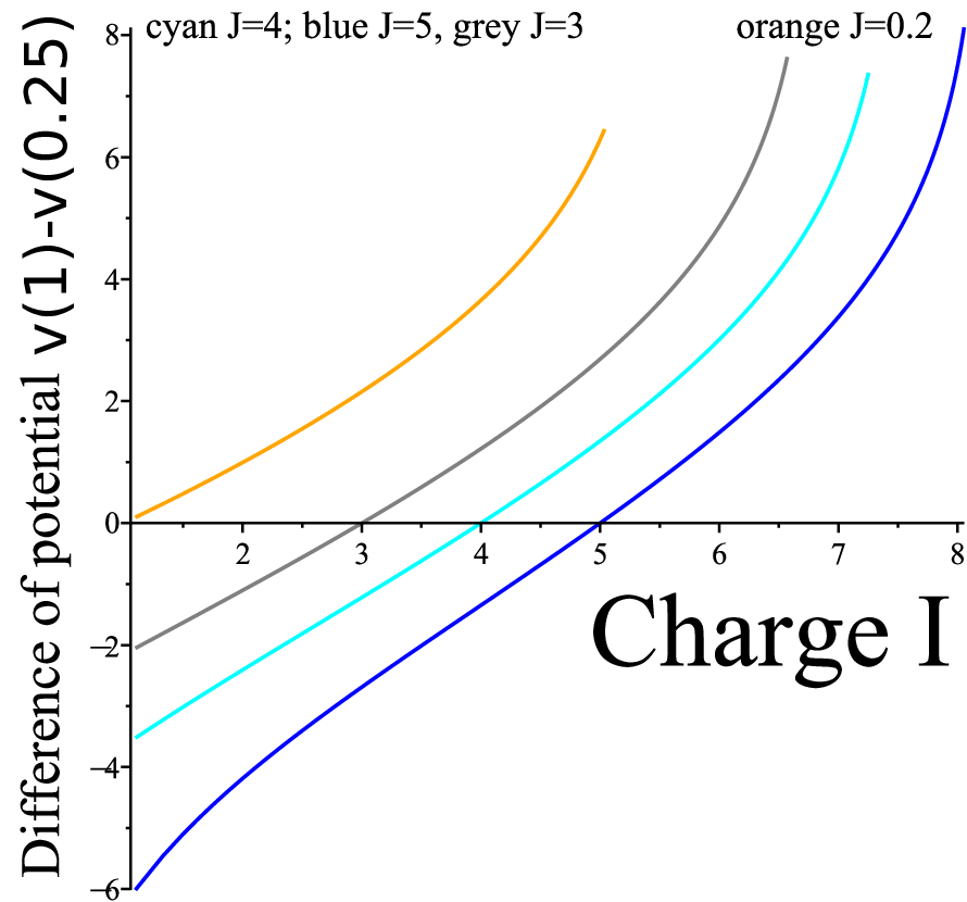
which does not have a direct solution. We solved numerically eq. 79 with boundary conditions 21 (Fig. 8).

6 Discussion and concluding remarks

We have studied in this article the distribution of the voltage field in a global but non-local electroneutral electrolyte. We found that the voltage does not decay quickly, but quite slowly inside the bulk region due to the local charge imbalance. We could completely resolve the electrodiffusion equations in dimension one (flat geometry) and partially in dimension 2 (cylindrical) using a regular perturbation around the solution with positive ions only and a negative charge in a disk. The solution in dimension three could only be estimated numerically. In all three dimensions, the potential difference between the inner and outer surfaces of the electrolyte should depend on the log of the charges, as we have shown in dimensions 1 and 2 (see table 1). It will be interesting to extend the present analysis to the case of non-concentric disk and in particular to examine the situation where the inner and outer boundaries could be very close. We also expect that curved membrane will create voltage drops, as shown in [17] the case of global non-electroneutrality.
In many biological nanodomains, such as inside dendritic spines, the concentration of mobile chloride ions is not counterbalanced by the mobile positive ions (potassium, sodium and free calcium ions essentially). For a total of 150 $mM$ positive, the mobile ions are divided into $~18$ mM $Na+$ , $~135mMK+$ and $~0.0001mMCa2+$ and $~7mMCl-$ ions and it is expected that most negative charges are located in membranes and consist of almost immobile macromolecules. These differences in ion mobility might result in important junction potentials (that is, local depletions in specific ion species), especially during transient synaptic activation, following an important influx of positive charges through AMPA-type glutamate receptors. In the present model, if we consider $n_{+}=150mM$ $n_{-}=7mM$ $N=143$ in a ball of $1\mu m$ and an inner domain of $100nm$ , then using the dimension 1 approximation for $N\approx 10^{8},n+\approx 9.10^{7}\gg 1$ and $n-\approx 44.10^{5}$ , we have from eq. 64 that

\displaystyle u(1)-u(a)\sim 2\ln\left(\sqrt{\lambda_{d}(1-a)}\frac{N}{\sqrt{n^{-}}}\right)=0.167

(80)

where $\lambda_{d}=6.97*10^{-10}$ , $a=0.25$ and the parameters are given in table 2. Thus the voltage difference is $\Delta V=4.33mV$ in a region of length 750nm.

Table 2: Parameters.

Parameter	Description	Value
$z$	Valence of ion	z=1 (for sodium)
$\Omega$	Spine head	$\Omega$ (volume $\|\Omega\|=1\mu m^{3}$ )
$a$	size of the negative charge region	(typical) $a=0.25\mu m$
$R$	radius of spine head	(typical) $L=1\mu m$
$T$	Temperature	$T=300K$
$E$	Energy	$kT=2.58\times 10^{-2}eV$
$e$	Electron charge	$e=1.6\times 10^{-19}C$
$\varepsilon$	Dielectric constant	$\varepsilon=80$
$\varepsilon_{0}$	Dielectric constant	$\varepsilon=8.85*10^{-12}F/m$

Finally, this study pushes to test the spatial limit of the electro-neutrality hypothesis in neuronal cell. When a large amount of negatively charged proteins are distributed in a confined microdomain, it would be interesting to investigate the consequences on the regulation of positive ionic distribution entering through channels. In particular, we expect from the present study that injecting a current in a cell when electroneutrality is not satisfied at a scale of $10$ to $100nm$ , will lead to long penetrating voltage drop inside the bulk.
After sodium positive ions enter a dendritic spine, other positive potassium ions could be expelled quickly, a process that would not happen if positive and negative charges would enter at the same time. A transient entry of positive ions in a non-electroneutrality medium could thus generate an electric field much further away compared to an electroneutrality medium, possibly responsible for the fast propagation of opening and closing of channels along dendrites and axons, a mechanism that could also challenge the classical Hodgkin-Huxley paradigm.

7 Appendices

7.1 Direct integration

We solve eq. 22 by a direct integration after multiplying by $u^{\prime}(x)$ equation

\displaystyle u^{\prime\prime}(x)=I_{\lambda}e^{u(x)}-J_{\lambda}e^{-u(x)}\qquad\text{for $a<x<1$},

(81)

we get

\displaystyle\frac{1}{2}u^{\prime 2}(x)=I_{\lambda}e^{u(x)}+J_{\lambda}e^{-u(x)},

(82)

where we used the boundary conditions

\displaystyle u(1)=0,\quad u^{\prime}(1)=0.

(83)

We now set $u(x)=v(x)+D$ with $D=\frac{1}{2}\ln\left(\frac{J_{\lambda}}{I_{\lambda}}\right)\geq 0$ and get

\displaystyle v^{\prime 2}(x)=A(\cosh(v(x))+c),

(84)

where

\displaystyle A=4\sqrt{I_{\lambda}J_{\lambda}}\quad,\quad c=-\frac{I_{\lambda}+J_{\lambda}}{2\sqrt{I_{\lambda}J_{\lambda}}}.

(85)

In order to integrate eq.(84), we compute the integral

\displaystyle I(v)=\int^{v}\frac{du}{\sqrt{\cosh(u)+c}}=\int^{v}\frac{du}{\sqrt{2\cosh^{2}(\frac{u}{2})-1+c}}.

(86)

Changing the variable $x=\frac{1}{\cosh(\frac{v}{2})}$ , we transform integral 86 into

\displaystyle I(v)=-2\mathop{\text{\huge$\int^{\text{\normalsize$\scriptstyle\frac{\displaystyle 1}{\displaystyle\cosh\left(\frac{v}{2}\right)}$}}$}}\nolimits\frac{\displaystyle dx}{\displaystyle\sqrt{(1-x^{2})\left(2-(1-c)x^{2}\right)}}.

(87)

We define

\displaystyle k=\sqrt{\frac{2}{1-c}}=\frac{\displaystyle 2\sqrt[4]{I_{\lambda}J_{\lambda}}}{\displaystyle\sqrt{I_{\lambda}}+\sqrt{J_{\lambda}}},\qquad 0<k\leq 1

(88)

and set $x=kt$ to obtain the incomplete elliptic integral of the first kind of amplitude $\frac{1}{kcosh\left(\frac{u}{2}\right)}$ and modulus $k$ (eq.(88) leads to $0<k\leq 1$ ):

\displaystyle I(v)=-\sqrt{2}k\mathop{\text{\huge$\int^{\text{\normalsize$\scriptstyle\frac{\displaystyle 1}{\displaystyle k\cosh\left(\frac{v}{2}\right)}$}}$}}\nolimits\frac{\displaystyle dt}{\displaystyle\sqrt{(1-k^{2}t^{2})(1-t^{2})}}=K\left(\frac{1}{k\cosh\left(\frac{v}{2}\right)},k\right).

(89)

Thus from eq.(84), we get

\displaystyle K\left(\frac{1}{k\cosh\left(\frac{v(x)}{2}\right)},k\right)=\alpha-\sqrt{\frac{A}{2}}\frac{x}{k},

(90)

where $\alpha$ is a constant. Since $u(1)=0$ , $v(1)=-D$ thus $\cosh\left(\frac{v(1)}{2}\right)=\frac{1}{k}$ and $\alpha=K(1,k)+\sqrt{\frac{A}{2}}\frac{1}{k}$ . Using the Jacobian elliptic functions of modulus $k$ , we obtain the explicit expression for $v$ with respect to $x$ using the identity $K(.,k)=\operatorname{sn}^{-1}(.)$ . Finally,

\displaystyle\frac{1}{k\cosh\left(\frac{v(x)}{2}\right)}=\operatorname{sn}\left(K(1,k)+\sqrt{\frac{A}{2}}\frac{1-x}{k}\right)=\operatorname{cd}\left(\sqrt{\frac{A}{2}}\frac{x-1}{k}\right),

(91)

and $v(x)\leq 0$ for $a\leq x\leq 1$ ,

\displaystyle v(x)=-2\operatorname{arcosh}\left[\frac{1}{k}\operatorname{dc}\left(\sqrt{\frac{A}{2}}\frac{x-1}{k}\right)\right].

(92)

In the following part, we will write $K(k)=K(1,k)$ the complete elliptic integral of the first kind. The normalize potential is

\displaystyle u(x)=-2\ln\left(\frac{1}{2}\frac{\sqrt{I_{\lambda}}+\sqrt{J_{\lambda}}}{\sqrt{J_{\lambda}}}\left(\operatorname{dc}\left(\frac{\sqrt{I_{\lambda}}+\sqrt{J_{\lambda}}}{\sqrt{2}}(x-1)\right)+\sqrt{1-k^{2}}\operatorname{nc}\left(\frac{\sqrt{I_{\lambda}}+\sqrt{J_{\lambda}}}{\sqrt{2}}(x-1)\right)\right)\right).

(93)

7.2 Appendix 2: classical relations between elliptic functions

The incomplete elliptic integral of the first kind of modulus $k$ and argument $x$ is defined by

\displaystyle K(x,k)=\int_{0}^{\phi}\frac{d\theta}{\sqrt{1-k^{2}\sin^{2}(\theta)}}=\int_{0}^{x}\frac{dt}{\sqrt{(1-t^{2})(1-k^{2}t^{2})}},

(94)

where $x=\sin\phi$ . For $x=1$ , we obtain the complete elliptic integral of modulus $k$ :

\displaystyle K(k)=\int_{0}^{1}\frac{dt}{(1-t^{2})(1-k^{2}t^{2})}

(95)

The elliptic sine $sn$ of modulus $k$ and the elliptic cosine $cn$ of modulus $k$ are defined by

\displaystyle sn(K(x,k),k)=\sin\phi=x,\quad cn(K(x,k),k)=\cos\phi.

(96)

We shall omit the $k$ argument so that $sn(u,k)=sn(u)$ . The delta amplitude is defined by

\displaystyle dn(u)=\sqrt{1-k^{2}sn(u)}.

(97)

The other nine Jacobian elliptic functions are obtained as ratios of the three first ones, following the formula

\displaystyle pq(u)=\frac{pn(u)}{qn(u)},

(98)

where $p$ and $q$ are any of the letter $n$ , $s$ , $c$ , $d$ , and $nn(u)=1$ . For example,

\displaystyle sc(u)=\frac{sn(u)}{cn(u)}\quad\text{and}\quad nc(u)=\frac{1}{cn(u)}.

(99)

Squares of the functions are obtained from the two relations :

	$\displaystyle sn^{2}(u)+cn^{2}(u)$	$\displaystyle=1,$			(100)
	$\displaystyle(1-k^{2})sn^{2}(u)+cn^{2}(u)$	$\displaystyle=dn^{2}(u).$			(101)

7.3 Relations between parameters $I_{\lambda}$ and $J_{\lambda}$

We provide here expressions between $I_{\lambda}$ and $J_{\lambda}$ : since $\operatorname{arcosh}(x)=\ln\left(x+\sqrt{x^{2}-1}\right)$ for $x\geq 1$ , we have

\displaystyle e^{-v(x)}=\left(\frac{1}{k}\operatorname{dc}\left(\sqrt{\frac{A}{2}}\frac{x-1}{k}\right)+\sqrt{\frac{1}{k^{2}}\operatorname{dc}^{2}\left(\sqrt{\frac{A}{2}}\frac{x-1}{k}\right)-1}\right)^{2}.

(102)

Using the modulus $k$ of the Jacobian elliptic function $dc$ , we have $dc^{2}(u)-k^{2}=(1-k^{2})\operatorname{nc}^{2}(u)$ and then

\displaystyle e^{-v(x)}=\left(\frac{1}{k}\operatorname{dc}\left(\sqrt{\frac{A}{2}}\frac{x-1}{k}\right)+\frac{\sqrt{1-k^{2}}}{k}\operatorname{nc}\left(\sqrt{\frac{A}{2}}\frac{x-1}{k}\right)\right)^{2}.

(103)

We expand this expression and use the following integrals

	$\displaystyle\int^{u}\operatorname{dc}^{2}(x)dx=-E(u)+u+\operatorname{sn}(u)\operatorname{dc}(u),$	(104)
	$\displaystyle\int^{u}\operatorname{nc}(x)\operatorname{dc}(x)dx=\operatorname{sc}(u),$	(105)
$\displaystyle\left(1-k^{2}\right)$	$\displaystyle\int^{u}\operatorname{nc}^{2}(x)dx=-E(u)+\left(1-k^{2}\right)u+\operatorname{sn}(u)\operatorname{dc}(u),$	(106)

where $E$ is the incomplete elliptic integral of the second kind of modulus $k$ ,

\displaystyle E(u)=\int_{0}^{sn(u)}\sqrt{\frac{1-k^{2}x^{2}}{1-x^{2}}}dx.

(107)

This leads to

	$\displaystyle\int_{a}^{1}e^{-v(x)}dx=\frac{1}{k}\sqrt{\frac{2}{A}}\left(2\operatorname{E}(u_{a})-2\operatorname{sn}(u_{a})\operatorname{dc}(u_{a})-\left(2-k^{2}\right)u_{a}-2\sqrt{1-k^{2}}\operatorname{sc}(u_{a})\right),$		(108)
	$\displaystyle\text{with }u_{a}=\sqrt{\frac{A}{2}}\frac{a-1}{k}=\frac{\sqrt{I_{\lambda}}+\sqrt{J_{\lambda}}}{\sqrt{2}}(a-1).$		(109)

Then we compute the second integral

$\displaystyle\int_{a}^{1}e^{v(x)}dx$	$\displaystyle=\int_{a}^{1}\frac{dx}{\left(\frac{1}{k}\operatorname{dc}\left(\sqrt{\frac{A}{2}}\frac{x-1}{k}\right)+\frac{\sqrt{1-k^{2}}}{k}\operatorname{nc}\left(\sqrt{\frac{A}{2}}\frac{x-1}{k}\right)\right)^{2}}$	(110)
	$\displaystyle=k^{3}\sqrt{\frac{2}{A}}\int_{u_{a}}^{0}\frac{du}{\left(\operatorname{dc}(u)+\sqrt{1-k^{2}}\operatorname{nc}(u)\right)^{2}}$	(111)
	$\displaystyle=k^{3}\sqrt{\frac{2}{A}}\int_{u_{a}}^{0}\frac{\left(\operatorname{dc}(u)-\sqrt{1-k^{2}}\operatorname{nc}(u)\right)^{2}}{\left(\operatorname{dc}^{2}(u)-(1-k^{2})\operatorname{nc}^{2}(u)\right)^{2}}du.$	(112)

Since $dc^{2}(u)-(1-k^{2})nc^{2}(u)=k^{2}$ , we finally obtain

\displaystyle\int_{a}^{1}e^{v(x)}dx=\frac{1}{k}\sqrt{\frac{2}{A}}\int_{u_{a}}^{0}\left(\operatorname{dc}(u)-\sqrt{1-k^{2}}\operatorname{nc}(u)\right)^{2}du,

(113)

which is very similar to the previous integral eq.(102). We thus compute eq.(114) similarly, leading to

\displaystyle\int_{a}^{1}e^{v(x)}dx=\frac{1}{k}\sqrt{\frac{2}{A}}\left(2\operatorname{E}(u_{a})-2\operatorname{sn}(u_{a})\operatorname{dc}(u_{a})-\left(2-k^{2}\right)u_{a}+2\sqrt{1-k^{2}}\operatorname{sc}(u_{a})\right).

(114)

We define for $u\in]-K(k);K(k)[$

	$\displaystyle f(u)$	$\displaystyle=2\operatorname{E}(u)-(2-k^{2})u-2\operatorname{sn}(u)\operatorname{dc}(u),$			(115)
	$\displaystyle g(u)$	$\displaystyle=2\operatorname{sc}(u),$			(116)

so we can now write eq.(114) and eq.(108)

	$\displaystyle\int_{a}^{1}e^{v(x)}dx$	$\displaystyle=\frac{1}{k}\sqrt{\frac{2}{A}}\left(f(u_{a})+\sqrt{1-k^{2}}g(u_{a})\right),$			(117)
	$\displaystyle\int_{a}^{1}e^{-v(x)}dx$	$\displaystyle=\frac{1}{k}\sqrt{\frac{2}{A}}\left(f(u_{a})-\sqrt{1-k^{2}}g(u_{a})\right).$			(118)

Because $u=v+D$ we have

	$\displaystyle\int_{a}^{1}e^{v}=e^{-D}\int_{a}^{1}e^{u}=\sqrt{\frac{I_{\lambda}}{J_{\lambda}}}\frac{\lambda_{d}n^{-}}{I_{\lambda}}=\frac{\lambda_{d}n^{-}}{\sqrt{I_{\lambda}J_{\lambda}}},$		(119)
	$\displaystyle\int_{a}^{1}e^{-v}=e^{D}\int_{a}^{1}e^{-u}=\sqrt{\frac{J_{\lambda}}{I_{\lambda}}}\frac{\lambda_{d}n^{+}}{J_{\lambda}}=\frac{\lambda_{d}n^{+}}{\sqrt{I_{\lambda}J_{\lambda}}},$		(120)

and from eq.(85) and eq.(88) we obtain

\displaystyle\frac{1}{k}\sqrt{\frac{2}{A}}=\frac{\sqrt{I_{\lambda}}+\sqrt{J_{\lambda}}}{2\sqrt{2I_{\lambda}J_{\lambda}}}\quad\text{and}\quad\sqrt{1-k^{2}}=\frac{\sqrt{J_{\lambda}}-\sqrt{I_{\lambda}}}{\sqrt{I_{\lambda}}+\sqrt{J_{\lambda}}},

(121)

which finally gives the system


$\displaystyle\lambda_{d}n^{-}$	$\displaystyle=\frac{\sqrt{I_{\lambda}}+\sqrt{J_{\lambda}}}{2\sqrt{2}}\left(f(u_{a})+\frac{\sqrt{J_{\lambda}}-\sqrt{I_{\lambda}}}{\sqrt{I_{\lambda}}+\sqrt{J_{\lambda}}}g(u_{a})\right),$	(122a)
$\displaystyle\lambda_{d}n^{+}$	$\displaystyle=\frac{\sqrt{I_{\lambda}}+\sqrt{J_{\lambda}}}{2\sqrt{2}}\left(f(u_{a})-\frac{\sqrt{J_{\lambda}}-\sqrt{I_{\lambda}}}{\sqrt{I_{\lambda}}+\sqrt{J_{\lambda}}}g(u_{a})\right).$	(122b)

We can also notice that

\displaystyle\lambda_{d}N=-\frac{\sqrt{J_{\lambda}}-\sqrt{I_{\lambda}}}{\sqrt{2}}g(u_{a}).

(123)

7.4 Appendix: Computing the leading order term $u_{0}$ in dimension 2

The first term $u_{0}$ is the solution of

	$\displaystyle u_{0}^{\prime\prime}(r)+\frac{1}{r}u_{0}^{\prime}(r)$	$\displaystyle=$	$\displaystyle-J_{\lambda}e^{-u_{0}(r)},$		(124)
	$\displaystyle u_{0}(1)=u_{0}^{\prime}(1)$	$\displaystyle=$	$\displaystyle 0,$		(125)

which we obtained by setting $\delta=0$ in eq.(66). Using the change of variables

\displaystyle r

\displaystyle=e^{-t}\,\tilde{u}(t)

\displaystyle=u(r)+2t,

(126)

eq.(66) reduces to

\displaystyle\tilde{u}^{\prime\prime}(t)=-J_{\lambda}e^{-\tilde{u}(t)},

(127)

with boundary conditions

\displaystyle\tilde{u}(0)=0,\quad\tilde{u}^{\prime}(0)=2.

(128)

We resolve here

\displaystyle\frac{1}{2}\tilde{u}^{\prime 2}=J_{\lambda}e^{-\tilde{u}(t)}+2-J_{\lambda}.

(129)

in the three cases $J_{\lambda}<2$ , $J_{\lambda}=2$ and $J_{\lambda}>2$ .

Case $J_{\lambda}<2$

We integrate

\displaystyle I(\tilde{u})=\int^{\displaystyle\tilde{u}}\frac{dx}{\sqrt{J_{\lambda}e^{-x}+2-J_{\lambda}}}=\frac{2}{\sqrt{2-J_{\lambda}}}\int^{\sqrt{\frac{2-J_{\lambda}}{J_{\lambda}}}\exp(\frac{\tilde{u}}{2})}\frac{dv}{\sqrt{1+v^{2}}}.

(130)

leading to

\displaystyle\sqrt{\frac{2}{2-J_{\lambda}}}\operatorname{arsinh}\left(\sqrt{\frac{2-J_{\lambda}}{J_{\lambda}}}\exp\left(\frac{\tilde{u}}{2}\right)\right)=t+C,

(131)

where $C=\sqrt{\frac{2}{2-J_{\lambda}}}\operatorname{arsinh}\left(\sqrt{\frac{2-J_{\lambda}}{J_{\lambda}}}\right)$ . This leads to the simplified relation

\displaystyle u(r)=2\ln\left(\frac{1}{2}\left(1+\frac{1}{p}\right)r^{1-p}-\frac{1}{2}\left(\frac{1}{p}-1\right)r^{1+p}\right),

(132)

where $p=\sqrt{\frac{2-J_{\lambda}}{2}}$ . To evaluate how $J_{\lambda}$ depends on $\lambda_{d}n^{+}$ , we compute the integral in eq.(20) :

	$\displaystyle\int_{a}^{1}e^{-u(r)}rdr$	$\displaystyle=\displaystyle\mathop{\text{\Large$\int_{\text{\normalsize$\scriptstyle\kern-1.63885pta$}}^{\text{\normalsize$\scriptstyle 1$}}$}}\nolimits\frac{rdr}{\left(\frac{1}{2}\left(1+\frac{1}{p}\right)r^{1-p}-\frac{1}{2}\left(\frac{1}{p}-1\right)r^{1+p}\right)^{2}}$
		$\displaystyle=\displaystyle 4p^{2}\int_{a}^{1}\frac{r^{2p-1}dr}{\left(p+1-(1-p)r^{2p}\right)^{2}}=\displaystyle\frac{1-a^{2p}}{\left(1+a^{2p}\right)p+1-a^{2p}}$

and

\displaystyle\lambda_{d}n^{+}=\frac{J_{\lambda}\left(1-a^{2p}\right)}{\left(1+a^{2p}\right)p+1-a^{2p}}.

(133)

In the limit $p\longrightarrow 0$ , expanding $a^{2p}$ leads to

\displaystyle\lambda_{d}n^{+}\longrightarrow\frac{2\ln(a)}{\ln(a)-1}\quad\text{when}\quad J_{\lambda}\longrightarrow 2.

(134)

Case $J_{\lambda}=2$

When $J_{\lambda}=2$ , eq.(70) becomes

\displaystyle\frac{1}{2}\tilde{u}^{\prime 2}=2e^{-\tilde{u}},

(135)

thus

\displaystyle e^{\frac{\tilde{u}}{2}}\tilde{u}^{\prime}=2,

(136)

gives the solution

\displaystyle\tilde{u}(t)=2\ln(1+t).

(137)

Since $u(r)=\tilde{u}(-\ln(r))+2\ln(r)$ , we obtain the solution

\displaystyle u(r)=2\ln(r(1-\ln(r))).

(138)

We evaluate $\lambda_{d}n^{+}$ by computing the integral in eq.(20) :

\displaystyle\int_{a}^{1}e^{-u(r)}rdr=\mathop{\text{\Large$\int_{\text{\normalsize$\scriptstyle\kern-1.63885pta$}}^{\text{\normalsize$\scriptstyle 1$}}$}}\nolimits\frac{dr}{r\left(1-\ln(r)\right)^{2}}=\frac{\ln(a)}{\ln(a)-1},

(139)

and get

\displaystyle\lambda_{d}n^{+}=\frac{2\ln(a)}{\ln(a)-1}.

(140)

Case $J_{\lambda}>2$

Following 130, a direct integration leads to

\displaystyle I(\tilde{u})=\int^{\displaystyle\tilde{u}}\frac{dx}{\sqrt{J_{\lambda}e^{-x}-(J_{\lambda}-2)}}=\frac{2}{\sqrt{J_{\lambda}-2}}\int^{\sqrt{\frac{J_{\lambda}-2}{J_{\lambda}}}\exp(\frac{\tilde{u}}{2})}\frac{dv}{\sqrt{1-v^{2}}}.

(141)

Thus,

\displaystyle\sqrt{\frac{2}{J_{\lambda}-2}}\operatorname{arcsin}\left(\sqrt{\frac{J_{\lambda}-2}{J_{\lambda}}}\exp\left(\frac{\tilde{u}}{2}\right)\right)=t+C,

(142)

where $C=\sqrt{\frac{2}{J_{\lambda}-2}}\operatorname{arcsin}\left(\sqrt{\frac{J_{\lambda}-2}{J_{\lambda}}}\right)$ , leading to

\displaystyle u(r)=2\ln\left(r\left(\frac{1}{p}\sin(-p\ln(r))+\cos(-p\ln(r))\right)\right),

(143)

where $p=\sqrt{\frac{J_{\lambda}-2}{2}}$ . We can now evaluate the relation with $\lambda_{d}n^{+}$ in $J_{\lambda}$ , we compute the integral in eq.(20) :

\displaystyle\int_{a}^{1}e^{-u(r)}rdr=\int_{a}^{1}\frac{dr}{r\left(\frac{1}{p}\sin(-p\ln(r))+\cos(-p\ln(r))\right)^{2}}=\frac{1}{1-p\cot(p\ln(a))}

(144)

and

\displaystyle\lambda_{d}n^{+}=\frac{J_{\lambda}}{1-p\cot(p\ln(a))}.

(145)

Since $J_{\lambda}\longrightarrow 2$ , $p\longrightarrow 0$ and we obtain

\displaystyle\lambda_{d}n^{+}\longrightarrow\frac{2\ln(a)}{\ln(a)-1}\quad\text{when}\quad J_{\lambda}\longrightarrow 2.

(146)

In addition,

\displaystyle\lambda_{d}n^{+}\longrightarrow\infty\quad\text{when}\quad J_{\lambda}\longrightarrow J_{lim}(a),

(147)

where $J_{lim}(a)$ is the first positive solution of the equation

\displaystyle\sqrt{\frac{J-2}{2}}\cot\left(\sqrt{\frac{J-2}{2}}\ln(a)\right)=1.

(148)

7.5 Appendix: Computing the first term $u_{1}$ of the regular perturbation

The second term $u_{1}$ of the regular perturbation is the solution of

\displaystyle u_{1}^{\prime\prime}(r)+\frac{1}{r}u_{1}^{\prime}(r)=e^{u_{0}(r)}+J_{\lambda}e^{-u_{0}(r)}u_{1}(r),

(149)

with boundary conditions

\displaystyle u_{1}(1)=u_{1}^{\prime}(1)=0.

(150)

We distinguish three cases $J_{\lambda}<2$ , $J_{\lambda}=2$ and $J_{\lambda}>2$ . For $J_{\lambda}<2$ , the homogeneous equation is

\displaystyle u^{\prime\prime}(r)+\frac{1}{r}u^{\prime}(r)-\frac{8p^{2}(1-p^{2})}{r^{2}\left((p+1)r^{-p}-(1-p)r^{p}\right)^{2}}u(r)=0,

(151)

where $p=\sqrt{1-\frac{J_{\lambda}}{2}}$ . We use the change of variable $x=r^{p}$ and $u(r)=v(x)$ , to transform the equation into

	$\displaystyle v^{\prime\prime}(x)+\frac{1}{r}v^{\prime}(x)$	$\displaystyle-\frac{8q}{(q-x^{2})^{2}}v(r)=0,$			(152)
	$\displaystyle v(1)$	$\displaystyle=v^{\prime}(1)=0,$			(153)

where $q=\frac{1+p}{1-p}$ . The two independent solutions are

	$\displaystyle y_{1}(x)$	$\displaystyle=$	$\displaystyle\frac{x^{2}+q}{x^{2}-q},$		(154)
	$\displaystyle y_{2}(x)$	$\displaystyle=$	$\displaystyle y_{1}(x)\ln(x)-1,$		(155)

thus the solutions to eq.(151) are

	$\displaystyle Y_{1}(r)$	$\displaystyle=$	$\displaystyle\frac{r^{2p}+q}{r^{2p}-q},$		(156)
	$\displaystyle Y_{2}(r)$	$\displaystyle=$	$\displaystyle pY_{1}(r)\ln(r)-1.$		(157)

Finally, the general solution of eq.(149) with initial conditions (150) is

\displaystyle u_{1}(r)=(\lambda(r)+A)Y_{1}(r)+(\mu(r)+B)Y_{2}(r),

(158)

where

$\displaystyle\mu(r)$	$\displaystyle=$	$\displaystyle\frac{(1-p)^{2}}{4p^{3}(4+2p)}r^{4+2p}-\frac{(1+p)^{2}}{4p^{3}(4-2p)}r^{4-2p},$	(159)
$\displaystyle\lambda(r)$	$\displaystyle=$	$\displaystyle-p\mu(r)\ln(r)-\frac{1-p^{2}}{8p^{3}}r^{4}+\frac{(1-p)^{2}(4+3p)}{4p^{3}(4+2p)^{2}}r^{4+2p}+\frac{(1+p)^{2}(4-3p)}{4p^{3}(4-2p)^{2}}r^{4-2p},$
$\displaystyle A$	$\displaystyle=$	$\displaystyle-\frac{1}{8}\frac{p^{4}-23p^{2}+40}{p(p^{2}-4)^{2}},\,B=-\frac{1}{4}\frac{p^{2}+5}{p^{2}(p^{2}-4)}.$

When $J_{\lambda}=2$ , eq.(74) becomes

\displaystyle u_{1}^{\prime\prime}(r)+\frac{1}{r}u_{1}^{\prime}(r)-\frac{2}{r^{2}(1-\ln(r))^{2}}u_{1}(r)=r^{2}(1-\ln(r))^{2}.

(160)

The solution is $u_{1}(r)=\left(A+\lambda(r)\right)\left(1-\ln(r)\right)^{2}+\frac{B+\mu(r)}{1-\ln(r)},$ where

$\displaystyle A$	$\displaystyle=$	$\displaystyle\frac{5}{48},\,B=-\frac{103}{384}$
$\displaystyle\lambda(r)$	$\displaystyle=$	$\displaystyle\frac{r^{4}}{12}\left(-\frac{5}{4}+\ln(r)\right)$
$\displaystyle\mu(r)$	$\displaystyle=$	$\displaystyle\frac{r^{4}}{384}\left(32\ln(r)^{4}-160\ln(r)^{3}+312\ln(r)^{2}-284\ln(r)+103\right).$

Finally, when $J_{\lambda}>2$ , the homogeneous eq.(74) is

\displaystyle u_{1}^{\prime\prime}(r)+\frac{1}{r}u_{1}^{\prime}(r)-\frac{2(1+p^{2})}{r^{2}\cos^{2}(p\ln(r))\left(1-\frac{1}{p}\tan(p\ln(r))\right)^{2}}u_{1}(r)=0,

(161)

where $p=\sqrt{\frac{J_{\lambda}}{2}-1}$ . We use the change of variable $x=\tan(p\ln(r))$ and $v(x)=u(r)$ to get

\displaystyle v^{\prime\prime}(x)+\frac{2x}{1+x^{2}}v^{\prime}(x)-\frac{2(1+p^{2})}{(p-x)^{2}(1+x^{2})}v(x)=0.

(162)

The independent solutions are

	$\displaystyle y_{1}(x)$	$\displaystyle=\frac{1+px}{x-p},$
	$\displaystyle y_{2}(x)$	$\displaystyle=y_{1}(x)\arctan(x)-1.$

Therefore the solutions to the homogenous eq. (161) are

	$\displaystyle Y_{1}(r)$	$\displaystyle=\displaystyle\frac{1+p\tan(p\ln(r))}{\tan(p\ln(r))-p},$			(163)
	$\displaystyle Y_{2}(r)$	$\displaystyle=pY_{1}(r)\ln(r)-1.$			(164)

Finally, the solution of eq.(74) with initial conditions (150) is

\displaystyle u_{1}(r)=(\lambda(r)+A)Y_{1}(r)+(\mu(r)+B)Y_{2}(r),

(165)

where

$\displaystyle\mu(r)$	$\displaystyle=$	$\displaystyle\frac{r^{4}}{p^{3}(16+4p^{2})}\left(\left(5p-p^{3}\right)\cos(2p\ln(r))-(2-4p^{2})\sin(2p\ln(r))\right),$
$\displaystyle\lambda(r)$	$\displaystyle=$	$\displaystyle-p\mu(r)\ln(r)-\frac{(1+p^{2})r^{4}}{8p^{3}}-\frac{7p^{4}+8p^{2}-8}{4p^{3}(p^{2}+4)^{2}}r^{4}\cos(2p\ln(r))$
	$\displaystyle-$	$\displaystyle\frac{3p^{4}-15p^{2}-36}{8p^{2}(p^{2}+4)^{2}}r^{4}\sin(2p\ln(r)),$
$\displaystyle A$	$\displaystyle=$	$\displaystyle\frac{1}{8}\frac{p^{4}+23p^{2}+40}{p(p^{2}+4)^{2}},$
$\displaystyle B$	$\displaystyle=$	$\displaystyle\frac{1}{4}\frac{p^{2}-5}{p^{2}(p^{2}+4)}.$

References

[1] B. Hille et al., Ion channels of excitable membranes, vol. 507. Sinauer Sunderland, MA, 2001.
[2] R. S. Eisenberg and E. A. Johnson, “Three-dimensional electrical field problems in physiology,” Progress in biophysics and molecular biology, vol. 20, pp. 1–65, 1970.
[3] F. Bezanilla, “How membrane proteins sense voltage,” Nature reviews Molecular cell biology, vol. 9, no. 4, p. 323, 2008.
[4] C. Koch and I. Segev, “Methods in neuronal modeling: From synapses to networks. 1989.”
[5] R. Yuste, Dendritic spines. MIT press, 2010.
[6] D. Holcman and R. Yuste, “The new nanophysiology: regulation of ionic flow in neuronal subcompartments,” Nature Reviews Neuroscience, vol. 16, no. 11, p. 685, 2015.
[7] S. Sylantyev, L. P. Savtchenko, Y. Ermolyuk, P. Michaluk, and D. A. Rusakov, “Spike-driven glutamate electrodiffusion triggers synaptic potentiation via a homer-dependent mglur-nmdar link,” Neuron, vol. 77, no. 3, pp. 528–541, 2013.
[8] K. Jayant, M. Wenzel, Y. Bando, J. P. Hamm, N. Mandriota, J. H. Rabinowitz, I. Jen-La Plante, J. S. Owen, O. Sahin, K. L. Shepard, et al., “Flexible nanopipettes for minimally invasive intracellular electrophysiology in vivo,” Cell reports, vol. 26, no. 1, pp. 266–278, 2019.
[9] K. Jayant, J. J. Hirtz, I. Jen-La Plante, D. M. Tsai, W. D. De Boer, A. Semonche, D. S. Peterka, J. S. Owen, O. Sahin, K. L. Shepard, et al., “Targeted intracellular voltage recordings from dendritic spines using quantum-dot-coated nanopipettes,” Nature nanotechnology, vol. 12, no. 4, p. 335, 2017.
[10] J. Cartailler, T. Kwon, R. Yuste, and D. Holcman, “Deconvolution of voltage sensor time series and electro-diffusion modeling reveal the role of spine geometry in controlling synaptic strength,” Neuron, vol. 97, no. 5, pp. 1126–1136, 2018.
[11] D. Gillespie, W. Nonner, and R. S. Eisenberg, “Coupling poisson–nernst–planck and density functional theory to calculate ion flux,” Journal of Physics: Condensed Matter, vol. 14, no. 46, p. 12129, 2002.
[12] Z. Schuss, B. Nadler, and R. Eisenberg, “Derivation of poisson and nernst-planck equations in a bath and channel from a molecular model,” Physical Review E, vol. 64, no. 3, p. 036116, 2001.
[13] P. Berg and J. Findlay, “Analytical solution of the poisson–nernst–planck–stokes equations in a cylindrical channel,” Proceedings of the Royal Society A: Mathematical, Physical and Engineering Sciences, vol. 467, no. 2135, pp. 3157–3169, 2011.
[14] P. Berg and K. Ladipo, “Exact solution of an electro-osmotic flow problem in a cylindrical channel of polymer electrolyte membranes,” Proceedings of the Royal Society A: Mathematical, Physical and Engineering Sciences, vol. 465, no. 2109, pp. 2663–2679, 2009.
[15] J. Cartailler, Z. Schuss, and D. Holcman, “Analysis of the poisson–nernst–planck equation in a ball for modeling the voltage–current relation in neurobiological microdomains,” Physica D: Nonlinear Phenomena, vol. 339, pp. 39–48, 2017.
[16] J. Cartailler, Z. Schuss, and D. Holcman, “Geometrical effects on nonlinear electrodiffusion in cell physiology,” Journal of Nonlinear Science, vol. 27, no. 6, pp. 1971–2000, 2017.
[17] J. Cartailler, Z. Schuss, and D. Holcman, “Electrostatics of non-neutral biological microdomains,” Scientific reports, vol. 7, no. 1, p. 11269, 2017.
[18] J. Cartailler and D. Holcman, “Steady-state voltage distribution in three-dimensional cusp-shaped funnels modeled by pnp,” Journal of mathematical biology, pp. 1–31, 2019.
[19] A. Singer and J. Norbury, “A poisson–nernst–planck model for biological ion channels—an asymptotic analysis in a three-dimensional narrow funnel,” SIAM Journal on Applied Mathematics, vol. 70, no. 3, pp. 949–968, 2009.
[20] M. Abramowitz and I. A. Stegun, Handbook of Mathematical Functions with Formulas, Graphs, and Mathematical Tables. Dover, New York, 1972.
[21] J. Cartailler, Z. Schuss, and D. Holcman, “Analysis of the poisson–nernst–planck equation in a ball for modeling the voltage–current relation in neurobiological microdomains,” Physica D: Nonlinear Phenomena, vol. 339, pp. 39–48, 2017.

Voltage distribution in a non-locally but globally electroneutral confined electrolyte medium: applications for nanophysiology

Abstract

1 Introduction

2 Model of global but not local electroneutrality

2.1 The Poisson-Nernst-Planck equations in the domain Ω\Omega

2.2 Steady-state solution

3 steady-state Solution of PNP eq.(19) in flat geometry (dimension 1)

3.1 Explicit expressions for the difference of potential u⁡(1)−u⁡(a)u(1)-u(a)

3.1.1 Case n−⟶0n^{-}\longrightarrow 0 (n+=Nn^{+}=N)

3.1.2 Case N=0N=0 (n+=n−n^{+}=n^{-})

3.1.3 Case ua≪1u_{a}\ll 1

3.1.4 Case ua⟶−K⁡(k)u_{a}\longrightarrow-K(k)

3.2 Summary potential difference u⁡(1)−u⁡(a)u(1)-u(a)

4 Steady-solution in two dimensions

4.1 No negative ions : Iλ=0I_{\lambda}=0

4.1.1 Regular perturbation solution for Iλ=ε≪1I_{\lambda}=\varepsilon\ll 1

5 Numerical evaluation of the voltage distribution in three dimensions

6 Discussion and concluding remarks

7 Appendices

7.1 Direct integration

7.2 Appendix 2: classical relations between elliptic functions

7.3 Relations between parameters IλI_{\lambda} and JλJ_{\lambda}

7.4 Appendix: Computing the leading order term u0u_{0} in dimension 2

Case Jλ<2J_{\lambda}<2

Case Jλ=2J_{\lambda}=2

Case Jλ>2J_{\lambda}>2

7.5 Appendix: Computing the first term u1u_{1} of the regular perturbation

References

2.1 The Poisson-Nernst-Planck equations in the domain $\Omega$

3.1 Explicit expressions for the difference of potential $u(1)-u(a)$

3.1.1 Case $n^{-}\longrightarrow 0$ ( $n^{+}=N$ )

3.1.2 Case $N=0$ ( $n^{+}=n^{-}$ )

3.1.3 Case $u_{a}\ll 1$

3.1.4 Case $u_{a}\longrightarrow-K(k)$

3.2 Summary potential difference $u(1)-u(a)$

4.1 No negative ions : $I_{\lambda}=0$

4.1.1 Regular perturbation solution for $I_{\lambda}=\varepsilon\ll 1$

7.3 Relations between parameters $I_{\lambda}$ and $J_{\lambda}$

7.4 Appendix: Computing the leading order term $u_{0}$ in dimension 2

Case $J_{\lambda}<2$

Case $J_{\lambda}=2$

Case $J_{\lambda}>2$

7.5 Appendix: Computing the first term $u_{1}$ of the regular perturbation