Spiral magnetic field and bound states of vortices in noncentrosymmetric superconductors
Abstract
We discuss the unconventional magnetic response and vortex states arising in noncentrosymmetric superconductors with chiral octahedral and tetrahedral ( or ) symmetry. We microscopically derive Ginzburg-Landau free energy. It is shown that due to spin-orbit and Zeeman coupling magnetic response of the system can change very significantly with temperature. For sufficiently strong coupling this leads to a crossover from type-1 superconductivity at elevated temperature to vortex states at lower temperature. The external magnetic field decay in such superconductors does not have the simple exponential law. We show that in the London limit, magnetic field can be solved in terms of complex force-free fields , which are defined by . Using that we demonstrate that the magnetic field of a vortex decays in spirals. Because of such behavior of the magnetic field, the intervortex and vortex-boundary interaction becomes non-monotonic with multiple minima. This implies that vortices form bound states with other vortices, antivortices, and boundaries.
I Introduction
Macroscopic magnetic and transport properties of superconductors have a significant degree of universality. For ordinary superconductors, the magnetic field behavior in the simplest case is described by the London equation London 1961; Tinkham 2004; Svistunov et al. 2015
| (1) |
This dictates that an externally applied magnetic field decays exponentially in the superconductor at the characteristic length scale called magnetic field penetration length . The equation relating the supercurrent to magnetic field dictates that the supercurrent should decay with the same exponent. Within the standard picture, this type of behavior describes the magnetic field near superconducting boundaries and in vortices, with microscopic detail, only affecting the coefficient . The single length scale associated with magnetic field behavior enables the Ginzburg-Landau classification of superconductors Landau and Ginzburg 1950 by a single parameter: the ratio of to the coherence length (the characteristic length scale of density variation ). Within this classification, there are two types of superconductors, the type-II, that exist for allows stable vortices that interact repulsively and in the type-I, the vortices interact attractively and are not stable. However, a simple two-length-scales-based classification of superconducting states cannot be complete. One counter-example is multi-component materials, where there are several coherence lengths Babaev and Speight 2005; Silaev and Babaev 2011; Carlström et al. 2011a; Carlström et al. 2011b; Babaev et al. 2017. Moreover, there can be several magnetic field penetration lengths Silaev et al. 2018. This multiscale physics gives nontrivial intervortex interaction and results in distinct magnetic properties.
How universal is the magnetic response in single-component systems? Here we focus on magnetic and vortex properties of single-component systems in a crystal that lacks inversion symmetry. There are many discovered materials where superconductivity occurs in such crystals Bauer and Sigrist 2012; Yip 2014; Rebar et al. 2019; Shang et al. 2020; Hillier et al. 2009; Singh et al. 2020. Then the Eq. (1) does not necessarily apply since symmetry now allows for noncentrosymmetric terms.
Indeed Ginzburg-Landau (GL) free-energy functionals describing these, so-called noncentrosymmetric, superconducting systems were demonstrated to feature various new terms Bauer and Sigrist 2012. These include contributions that are linear in the gradients of the superconducting order parameter and the magnetic field . It principally revises the simplest London model Eq. (1) where such terms are forbidden on symmetry grounds. Depending on the symmetry of the material, the free energy can feature scalar and vector products of these fields of the form , where , , is the covariant derivative and is the order parameter, and are coefficients, which form depends on crystal symmetry Bauer and Sigrist 2012. Correspondingly, while in ordinary superconductors the externally applied field decays monotonically, in a Meissner state in a noncentrosymmetric superconductor it can have a spiral decay Bauer and Sigrist 2012; Levitov et al. 1985; Lu and Yip 2008a; Mineev and Samokhin 2008; Samokhin 2004; Samokhin and Mineev 2008; Lu and Yip 2008a. This raises the question of the nature of topological excitations in such materials Bauer and Sigrist 2012; Mineev and Samokhin 2008; Samokhin 2004; Samokhin and Mineev 2008; Lu and Yip 2008a; Lu and Yip 2008b; Kashyap and Agterberg 2013. The main goal of this paper is to investigate vortex solutions, their interaction, and the magnetic response of a superconductor where there is no inversion symmetry in an underlying crystal lattice.
I.1 The structure of the paper
In the Section II we discuss the microscopic derivation of the Ginzburg-Landau (GL) model. A reader who is not interested in technical details can proceed directly to the section Section III. In the Section III, by rescaling we cast the GL model in a representation that is more convenient for calculations and analysis. In the Section IV we describe a method that solves the hydromagnetostatics of a noncentrosymmetric superconductor in the London limit in terms of complex force-free fields. A reader not interested in the analytical detail can proceed directly to the next section. In Section V we obtain analytic and numerical vortex configuration with a spiral magnetic field. In Section VI we calculate the temperature dependence of the single vortex energy to show how a crossover to type-1 superconductivity appears at elevated temperatures in a class of noncentrosymmetric superconductors. In Section VII we consider intervortex forces and show that system forms vortex-vortex and vortex-antivortex bound states. In Section VIII we consider the problem of a vortex near a boundary of noncentrosymmetric superconductor and show that vortex forms bound states with it.
II Microscopic derivation of the Ginzburg-Landau model
Here we present a microscopic derivation of the GL model in the case of chiral octahedral or equivalently tetrahedral symmetry from the microscopic model. A reader, not interested in the technical derivation of the model can skip this section and directly proceed to the next sections that analyze the physical properties of the model.
II.1 Unbounded free energy in the minimal extension of the GL model
Typically quoted phenomenological GL models, have unphysical unboundedness of the energy from below ryb We thank Fillipp N. Rybakov for pointing that out. For example, the model presented in Chapter 5 of Bauer and Sigrist 2012 is given by energy density equal to usual GL model plus term. To see that energy is unbounded it is sufficient to consider constant and real order parameter . Then energy density is given by , where is potential. Consider the case of or symmetry given by . Then inserting Chandrasekhar-Kendall function Chandrasekhar and Kendall 1957 as we obtain energy density
| (2) |
which is unbounded from below. That can be seen as follows: by increasing and setting one obtains infinitely negative energy density. Similarly, consider for example, the case of symmetry, which corresponds to Rashba spin-orbit coupling . Then we can set . This leads to the same unbounded energy density Eq. (2).
The unboundedness of the model is associated with divergence of and . However, some of the previous works that derived the GL model assuming a finite uniform magnetic field Bauer and Sigrist 2012; Samokhin 2004; Samokhin 2014 obtained the term . This term in principle can make GL free energy bounded from below if the assumption of constant is lifted. Motivated by this problem we proceed to derive the GL model with nonuniform aiming to obtain a microscopically justified effective model with a bounded energy.
II.2 Microscopic model
We will focus on the simplest case with the BCS type local attractive interaction given by strength but will include a general space-dependent magnetic field . Interaction is regularized by Debye frequency such that only electrons with Matsubara frequency are interacting. We start from the continuous-space fermionic model in path integral formulation, given by the action and partition function :
| (3) |
where is temperature and are Grassman fields, which depend on imaginary time , three dimensional space coordinates and spin . They correspond to fermionic creation and annihilation operators and
| (4) |
where are Pauli matrices, is electron charge, is chemical potential and is Bohr magneton. Single electron energy is with , which is for quasi free electrons. However, in our derivation, we keep in general form, also suitable for band electrons. The only term responsible for noncentrosymmetric nature of the system is spin-orbit coupling .
Let us now consider the case of cubic or symmetry with simplest coupling . We will focus on the standard situation where the macroscopic length scale , over which the quantities change, is much larger than Fermi length scale , where is Fermi momenta. We assume that the following inequalities hold:
| (5) |
where is the critical temperature of a superconductor to a normal phase transition. We perform Hubbard-Stratonovich transformation by introducing auxiliary bosonic field . Hence, up to a constant, interaction term becomes:
| (6) |
Next, by introducing the partition function Eq. (3) can be written as:
| (7) |
where we have the matrix with
| (8) |
The symbol with a hat denotes matrices defined by and . Note, that for any function of operators , transposition is defined as . Integrating out fermionic degrees of freedom , by performing Berezin integration in Eq. (7), we obtain:
| (9) |
In the mean-field approximation, one assumes that doesn’t depend on (i.e. it’s classical) and doesn’t fluctuate thermally. Hence free energy is given by:
| (10) |
By Tr here and below we mean matrix trace tr and integration . To obtain the GL model we need to expand the second term in Eq. (10) in powers and derivatives of the field :
| (11) |
where the first equality is defined, up to constant in and , through:
| (12) |
Note, that in Eq. (11) matrices are multiplied and integrated inside the trace, for example, . Next we define
| (13) |
so that for slowly changing we get with . The Fourier transform for : is given by:
| (14) |
where is Matsubara frequency. Here we used the fact that only electrons with frequency smaller than Debye frequency are interacting, and that is a solution of the equation . By using the Fourier transformed we obtain:
| (15) |
where if . We can rewrite as:
| (16) |
where we use the notations and .
II.3 Minimal set of terms in the GL expansion for the noncentrosymmetric materials
II.3.1 Second-order terms
First, we examine the terms occurring in the second order. To that end, by using the Eq. (14) and substituting we compute term in Eq. (11) which is second order in :
| (17) |
where the operator is acting only on the gap field . The goal here is to simplify term in Eq. (17), where the prime ′ means dependence on . Hence using that we approximate
| (18) |
Then it is easy to show that up to the second order in and : and . Hence using Eq. (16) we obtain:
| (19) |
When summing over , contribution to integration over momenta in Eq. (17) mainly comes from a thin shell near Fermi momenta because the interaction is cut off by Debye frequency. This shell has the width .
| (20) |
where is the band index. Hence we can approximate . By using and , the integral in Eq. (17) can be estimated as:
| (21) |
where is density of states at Fermi level, is Fermi velocity and is solid angle. Then we perform integration and Matsubara sum in Eq. (17) by using Eq. (19), Eq. (21) and :
| (22) |
where and is digamma function. Next we expand in and average over in Eq. (22). Combining result with Eq. (17), Eq. (11), Eq. (10) and integrating by parts with , we obtain the part of the free energy which is second order in :
| (23) |
Note, that the kinetic term is split into two terms corresponding to different bands with covariant derivatives that apart from have . If one opens brackets – the only noncentrosymmetric term is proportional to difference of squares of Fermi momenta of two bands:
| (24) |
II.3.2 Fourth order term
As usual, at the fourth-order, it is sufficient to retain only term . Hence we neglect and difference in ’s. To that end we consider term in Eq. (11). By using Eq. (14) it can be written as
| (25) |
Here, to go to the second equality we used Eq. (16). By using the Eq. (25) and Eq. (10) we obtain the part of the free energy which is quartic in order parameter:
| (26) |
The principal difference between the GL model of centrosymmetric and noncentrosymmetric material here is in the form of the gradient term in Eq. (23). Note, that the frequently used phenomenological noncentrosymmetric GL models include only the cross term , that makes these models unbounded from below. The derived microscopic model solves this issue because the gradient term in Eq. (23) is a full square, i.e. is positively defined.
III Rescaling and parametric dependence of the microscopic GL model
In this section, we rescale the GL model to a simpler form that is analyzed below. The minimal, microscopically-derived GL model for noncentrosymmetric superconductor reads as a sum of second-order and fourth-order terms, given by Eq. (23) and Eq. (26):
| (27) |
Importantly, the energy of the model, derived here, is bounded from below i.e. the functional does not allow infinitely negative energy states. This is in contrast to the phenomenological model presented in Chapter 5 of Bauer and Sigrist 2012, which has artificial unboundedness of the energy from below ryb We thank Fillipp N. Rybakov for pointing that out.
The microscopically-derived model, can be cast in a more compact form by introducing the new variables and performing the following transformation:
| (28) |
After dropping the prime ′, the rescaled GL free energy can be written as:
| (29) |
where we define new parameters:
| (30) |
Two conclusions can be drawn here:
- •
The noncentrosymmetric term Eq. (24) has the prefactor that modifies the gradient term. It means that the sign of determines whether left or right-handed states are preferable. The term is proportional to microscopic spin-orbit coupling if . On the other hand, the parameter appears due to the coupling to the Zeeman magnetic field.
- •
The parameters are proportional to and hence for we get . Here is the critical temperature, defined in Eq. (23) so that . Note, that the characteristic parameter does not have the same meaning as the standard Ginzburg-Landau parameter. However, asymptotically, in the limit the noncentrosymmetric superconductor will behave as a usual superconductor with GL parameter .
Varying Eq. (29) with respect to , and we obtain the following Ginzburg-Landau (GL) equations:
| (31) |
with and boundary conditions for unitary vector orthogonal to the boundary:
| (32) |
IV An analytical approach for solutions in the London limit: Magnetic field configuration as the solution to the complex force-free equation
In this section, we develop an analytical method for treating Eq. (31). That will allow us to determine the magnetic field and current configurations in the London limit.
IV.1 Decoupling of fields at linear level
First we focus on asymptotic of the Eq. (31) over uniform background . Namely, we set and assume that and are small. By linearising the GL equations Eq. (31) in terms of them we obtain:
| (33) |
where . This is accompanied by the boundary conditions Eq. (32):
| (34) |
Note, that equation for the matter field has the same form as for usual superconductors. That allows us to define the coherence length as so that it parameterizes the exponential law how the matter field recovers from a local perturbation. Importantly the equation for and is decoupled from the equation for at the level of linearized theory. That means that the London limit is a fully controllable approximation for a noncentrosymmetric superconductor with short coherence length. Namely, when the length scale of density variation is much smaller than the characteristic length scale of the magnetic field decay and we are sufficiently far away from the upper critical magnetic field, so that vortex cores do not overlap, the London model is a good approximation.
IV.2 Analytical approach for solutions in the London limit in the presence of vortices.
In London approximation the order parameter is set to at to model a core of a vortex positioned at . Away from the core it recovers to bulk value .
Taking curl of the second equation in Eq. (33) we obtain equation that determines configuration of the magnetic field:
| (35) |
Far away from the vortex core, the right-hand side of Eq. (35) should be zero. By introducing a differential operator
| (36) |
Eq. (35) with zero right-hand side can be written as:
| (37) |
To simplify this equation we introduce complex force free field defined by or equivalently by . Using this and Eq. (37) we obtain that
| (38) |
where is arbitrary complex valued constant. Subtracting complex conjugated from Eq. (38) we obtain the solution for the magnetic field in terms of complex force free field :
| (39) |
Note, that we absorbed multiplicative complex constant into the definition of in the last step.
To obtain a solution for , one can solve the equation . However it is more elegant to employ the trick used by Chandrasekhar and Kendall Chandrasekhar and Kendall 1957. Namely, solution for is made of auxiliary functions:
| (40) |
There is freedom in choosing : it can be set to, for example, or . We note, that to make resulting equations simpler, if possible, it’s convenient to satisfy: , and . In this work we fix it to and hence set to:
| (41) |
In a London model a solution for a vortex is obtained by including a source term. Now if we take into account right-hand side of Eq. (35) second equation in Eq. (40) should be modified to include source term , which we define by . For multiple vortices with windings , placed at different positions , we have
| (42) |
The Eq. (35) with non zero right hand side can be written as:
| (43) |
This section can be summarized as follows: we justified taking the London limit by decoupling linearized matter field equation from magnetic field equation. We demonstrated that the equation Eq. (35), that determines magnetic field of superconductor in the London limit, can be simplified to:
| (45) |
Note, that this representation of in terms of complex force-free fields is general: i.e. it holds also for the usual centrosymmetric superconductor. But, as will be clear from the discussion below, it is particularly useful for noncentrosymmetric materials.
IV.3 Calculation of the free energy of nontrivial configurations
An example where the London model yields important physical information is vortex energy calculations. That allows determining for instance, lower critical magnetic fields and magnetization curves. Free energy Eq. (29), up to a constant, can be written as:
| (46) |
where is found from the second equation in Eq. (33) and curl of its definition . The formalism presented in this section allows a simple solution:
| (47) |
Hence energy of any configuration can be written as:
| (48) |
We will use the formalism of this section below to analyze the physical properties of noncentrosymmetric systems.
V Structure of a single vortex
V.1 Analytical treatment in the London limit
Earlier, vortex solutions were obtained only as a series expansion Bauer and Sigrist 2012; Lu and Yip 2008a, which didn’t exhibit any spiral structure of the magnetic field. In this section, we show how the method that we developed in Eq. (45) allows us to obtain an exact solution that turns out to be structurally different.
Consider a single vortex translationally invariant along direction and positioned at . Then in order to obtain magnetic field we need to solve second equation in Eq. (45):
| (50) |
Firstly, let’s solve it with zero right-hand side. Then Eq. (50) is just Helmholtz equation with complex parameter . In polar coordinates and its solution is . Where we chose – Hankel function of the first kind to obtain appropriate asymptotic for .
Next lets take into account right-hand side of Eq. (50). Since and for we obtain that . Hence only zero order Hankel function contributes to solution of Eq. (50), which is given by:
| (51) |
Hence using Eq. (51) and first line in Eq. (45), we obtain magnetic field of a vortex, see Fig. 1:
| (52) |

For this expression, as expected, gives the usual result . In polar coordinates Eq. (52) can be written as:
| (53) |
Then for since magnetic field forms the right handed spirals as in the case of the Meissner state, see below Eq. (57), but instead in a radial direction:
| (54) |
Note, that this is a general observation that decaying magnetic field forms a spiral with handedness determined by the sign of .
V.2 Vortex solution in the Ginzburg-Landau model.
To obtain the vortex solution in the full nonlinear Ginzburg-Landau model, we developed a numerical approach that minimizes the free energy Eq. (29). For that, we wrote code that uses a nonlinear conjugate gradient algorithm parallelized on CUDA enabled graphics processing unit, for detail of numerical approach see Samoilenka et al. 2020. The algorithm works as follows: firstly the fields and are discretized using a finite difference scheme on a Cartesian grid. Then energy is minimized by sequentially updating and in steps. In each step, we calculate gradients of the free energy with respect to the given field. Then we adjust the resulting vector with a nonlinear conjugate gradient algorithm, which gives the direction of the step in the field. Next, we expand energy in the Taylor series in terms of step amplitude for the obtained step direction. This amplitude is then calculated as a minimizer of the obtained polynomial and the step is made. Discretized grid had points. To verify results we used grids of different sizes like . The obtained numerical solutions of the full GL model Eq. (29) are shown on Fig. 2


In Fig. 3 we plot a comparison of the analytical solution obtained in the London model and the numerical solution in full nonlinear GL theory.
VI Crossover to type-1 superconductivity at elevated temperatures
In this section, we show how noncentrosymmetric superconductors can crossover from vortex states at low temperature to type-1 superconductivity at .
To that end, let us consider the energy of a single vortex with a core parallel to direction. Recall that first critical magnetic field is defined such that vortex energy becomes negative for . Namely, vortex energy (per unit length in direction) is given by , where is external magnetic field parallel to direction. Next, thermodynamic critical magnetic field is defined as when energy of the uniform superconducting state and is zero. In our rescaled units . In the usual type-II superconductors vortices form when . However, as we will see below, the interaction of vortices in this system is non-monotonic and hence lattice of vortices will become energetically beneficial for . Hence in order to show that superconductor has vortex states it is sufficient to find .
To observe a crossover consider a noncentrosymmetric superconductor that has . Then at , as we showed above, and hence it becomes usual type-1 superconductor described by the GL parameter . In this case and hence vortices are not present. However, when the temperature is decreased, and increase. By solving the full GL model Eq. (29), we find that this leads to a change in the value of . Eventually, it becomes smaller than at sufficiently low temperature, see Fig. 4. This means that vortices will necessarily start to appear.
Next, we study analytically how vortex states become energetically preferable. Firstly, consider the London limit, disregarding the vortex core energy. Using the previously obtained vortex solution Eq. (51) and energy given by Eq. (49), we obtain energy of a vortex with winding . We can express it in terms of the London limit first critical magnetic field :
| (55) |
where is Euler Gamma. For a single vortex we have . Let us estimate the core energy of a vortex. Since vortex core is of size then it is since and . Hence the actual first critical magnetic field can be estimated by . When this core energy is indeed relatively small and can be disregarded.
However, for studying a crossover to type-1 superconductivity Fig. 4, this is not true since . There, instead, the vortex core energy gives a significant contribution to . Numerically we estimated , see Fig. 4. Moreover, from Eq. (55) it follows that for the increased value of the vortex energy is dominated by core contribution. For the crossover to type-1 superconductivity we need and large enough value of .
Finally consider how parameters influence length scales over which order parameter and magnetic field change. Namely, we are interested in the ratio of these scales, since for usual superconductor it determines whether it is of type-1 or type-2. As we showed before, Eq. (33), coherence length has the usual form in a noncentrosymmetric superconductor. To obtain penetration depth one needs to solve for Meissner state in London limit. The Meissner state in the non-centrosymmetric superconductors was discussed before in Levitov et al. 1985; Lu and Yip 2008a; Bauer and Sigrist 2012 for similar models. Here we rederive it for our model Eq. (29) using the method that we outlined in the previous section Eq. (45).
Consider superconductor with no vortices occupying half-space and external magnetic field , parallel to the boundary. As usual, we assume that fields depend only on . Then the second equation in Eq. (45) is easily solved resulting in , since we demand , where is a complex multiplicative constant. To determine we use boundary condition Eq. (34), which in terms of becomes:
| (56) |
it gives , where . From Eq. (45) we obtain magnetic field, which can be represented by a linear combination of components of parallel to the boundary :
| (57) |

While the magnetic field has a spiral decay, its modulus has an exponential decay, see Fig. 5. That allows to define the penetration depth for magnetic field as the inverse of imaginary part of :
| (58) |
Importantly, inside a superconductor, the direction of the magnetic field rotates with the period , forming a right-handed spiral (helical) structure. This spiral is shown on Fig. 5. Note, that handedness of the state is set by the sign of . Also observe that the operator that determines the configuration of is invariant under inversion (parity) transformation and the model is centrosymmetric only if . It is also apparent from the fact that , where is, as was shown above, the parameter that determines the degree of noncentrosymmetry of the material.
The ratio of the magnetic field penetration length and coherence length for the noncentrosymmetric superconductor then reads
| (59) |
Note, that strongly depend on and go to zero for , see Eq. (30). Since the ratio increases when temperature is decreased, see Fig. 6. Hence it is typical that in noncentrosymmetric superconductors for . Namely, for the parameters in Fig. 4 we obtained that for , which is in strong contrast to centrosymmetric superconductors where for (or in different units). We show below that interaction between vortices is nonmonotonic and the critical field for vortex clusters is smaller than for a single vortex, and thus there is no Bogomolny point in the noncentrosymmetric superconductors considered in this paper.
We obtained crossover Fig. 4 and the Eq. (59) by considering a noncentrosymmetric superconductor with or symmetry. Noncentrosymmetric systems with different symmetry, have terms of different structure but with the same scaling, corresponding to spin-orbit and Zeeman coupling terms. It means that for any symmetry it is expected to have a strong dependence of these noncentrosymmetric terms on temperature. Consequently, if and terms are large enough, one can expect the crossover between different types in noncentrosymmetric superconductors. This type of behavior was reported for noncentrosymmetric superconductor AuBe Rebar et al. 2019.
VII Intervortex interaction and vortex bound states
Here we compute the interaction energy of vortices by using Eq. (49). Consider a set of vortices with windings placed at with cores parallel to . Then according to Eq. (45) and single vortex solution Eq. (51) satisfies:
| (60) |
Then by using the Eq. (60) and its complex conjugate we obtain the energy per unit length in direction:
| (61) |
where we also used that the flux of the vortices is fixed by . The integral in Eq. (61) is easily performed for any vortex combination since contains the Dirac delta’s in it. Now let us consider only two vortices . By subtracting from Eq. (61) energies of single vortices Eq. (55) we obtain the interaction energy as a function of distance between them:
| (62) |
Importantly, the intervortex interaction energy , see Fig. 7, changes sign. Analytically asymptotics for big is given by:
| (63) |
where . Hence the system forms vortex-vortex and vortex-antivortex pairs. Those will form stable states at distances corresponding to local minima in . Approximately (for big ) these minima appear with period . Note, that for period . Simplest estimate as minima/maxima of in Eq. (63) gives:
| (64) |
where is the distance between vortices, is the distance between vortex and antivortex and is an integer.
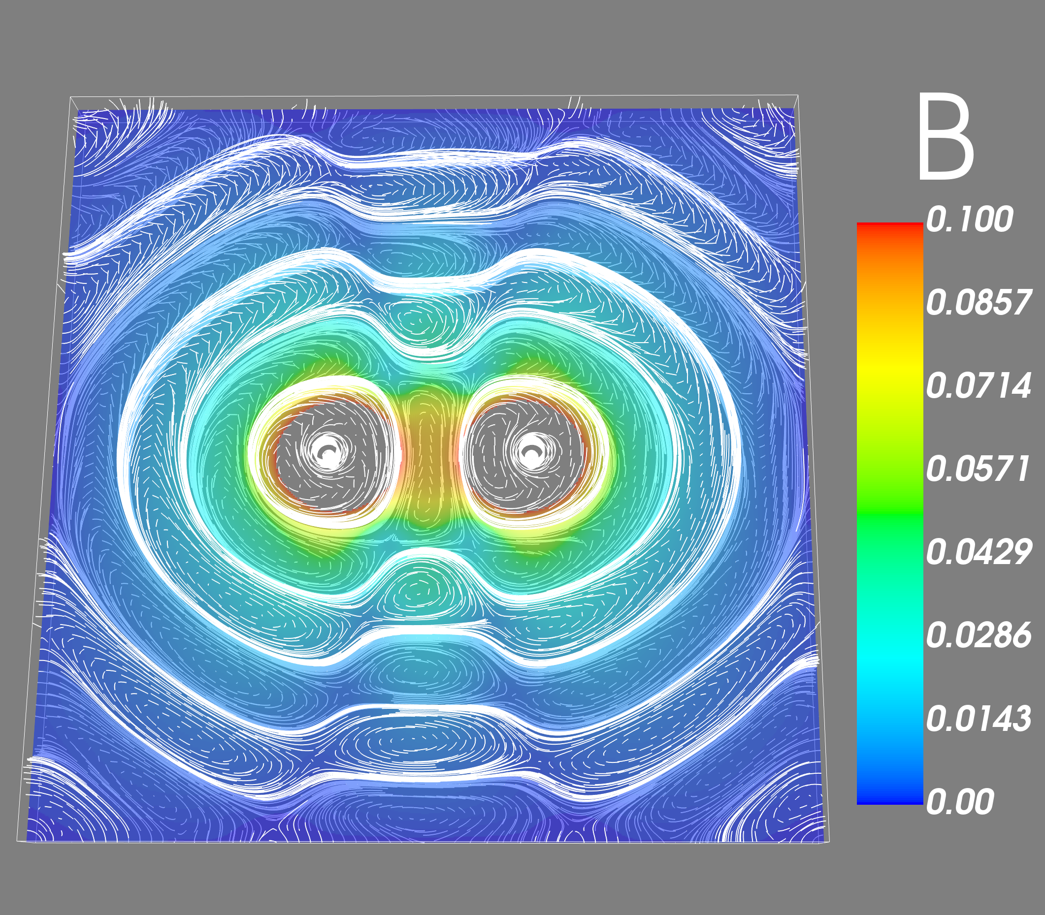
This behavior is due to the fact that in noncentrosymmetric superconductor vortices are represented by “circularly polarized” cylindrical magnetic field Eq. (52) with period approximately equal to , see Fig. 2 and Fig. 8. Two or more of them brought together will form an interference pattern of two-point sources which, when moving them apart, will alternate between in-phase and out of phase with the same period.
In the London limit, interaction can be easily generalized to an arbitrary number of vortices. Namely, using Eq. (61) pairwise interaction will be given by the same Eq. (62). Hence we can suggest that vortices can form lattices with the distance between neighboring vortices given by one of the minima of Eq. (62). Similarly, lattices of vortices and antivortices can be formed.
We obtained the bound states numerically in the full nonlinear GL model given by Eq. (29). The Fig. 8 shows two examples of such bound states.

VIII Vortex-boundary interaction
In this section, we show that in noncentrosymmetric superconductors physics of vortex-boundary interaction is unconventional. Consider a half infinite superconductor positioned at and right-handed vortex with winding placed at and . Here we study the problem in the London limit and thus neglect the effects associated with the gap variations near the surface Samoilenka and Babaev 2020, and the nonlinear effects appearing at the scale of the vortex core Benfenati et al. 2020. External magnetic field is set to be . Then auxiliary field should satisfy the following equation inside the superconductor Eq. (45):
| (65) |
supplemented by the boundary conditions that is zero at . From Eq. (34) or equivalently Eq. (56) we obtain the following boundary conditions at :
| (66) |
Since Eq. (65) is linear in it is convenient to write solution as superposition of Meissner state, vortex and image of a vortex as:
| (67) |
where and were found in the previous sections. Note, that since Meissner state satisfies boundary conditions Eq. (66), the vortex and image should satisfy Eq. (66) with zero right hand side.
Remember that with the London model, for usual superconductor image of the vortex is just its mirror reflection in the boundary, which is modeled by antivortex positioned outside the superconductor, see Bean and Livingston 1964. This configuration then satisfies both equation Eq. (65) and boundary conditions Eq. (66). By contrast in our case for noncentrosymmetric superconductor unfortunately it is not possible to use this approach. Namely, mirror reflection of right-handed vortex inside the superconductor is left-handed antivortex outside, which indeed satisfies boundary conditions Eq. (66), but equation for Eq. (35) (more complicated version of Eq. (65)) is not satisfied. This is simply because antivortex is left-handed but the equation is right-handed, or vice versa for . Inserted as an image right-handed anti-vortex satisfies Eq. (65), but not boundary conditions Eq. (66).
So to obtain an “image” configuration we have to solve explicitly the Eq. (65). We did that by performing Fourier transform in direction and solving corresponding equations Eq. (65) for together subjected to boundary condition Eq. (66) with zero right-hand side, which gives:
| (68) |
where we obtain, compared to Eq. (61), the last term which is boundary integral. Now inserting solutions Eq. (67) and Eq. (68) up to constant terms we obtain energy of a vortex interacting with a boundary, see Fig. 9:
| (70) |
where is energy of a single vortex in the bulk of superconductor Eq. (55) and other terms represent interaction energy of vortex and boundary. For a large distance away from the boundary , the main contribution to the interaction energy comes from first term in Eq. (70) and hence it has similar asymptotics as for vortex vortex interaction, namely we obtain , which has minimums with period , see Fig. 9.
Physically it means that the vortex-surface interaction in a noncentrosymmetric superconductor is principally different from that in an ordinary one. Namely, in the latter case the interaction with a boundary is a barrier-like for non-zero fields and attractive for zero and inverted fields Bean and Livingston 1964; Kramer 1968; Kramer 1973; de Gennes 1964; Benfenati et al. 2020. By contrast, we found that in a noncentrosymmetric superconductor vortices should form a bound state with a boundary. Then in increasing magnetic field vortices will first tend to stick near the boundary and only when there will be a considerable amount of them occupying these minima vortices will be pushed into the bulk of superconductor in the form of multi-vortex bound state.
For in the second term in Eq. (70) corresponds to an antivortex as in Bean and Livingston 1964. But physical interpretation in Bean and Livingston 1964 of the first term in Eq. (70) as Meissner-vortex and the second term as vortex-image interactions is not fully justified. Firstly, when integrating by parts energy Eq. (49) these terms are obtained from combining energy and flux from the field configuration of vortex and image. Secondly, half of the first term in Eq. (70) comes from boundary integral in Eq. (69) due to vortex-image interaction.
IX Conclusions
We considered the physics of magnetic field behavior and vortex states in noncentrosymmetric superconductors. We microscopically derived a Ginzburg-Landau model for noncentrosymmetric superconductors which does not suffer from unphysical ground state instability, which was present in frequently used phenomenological models. The main conclusion of the microscopic part of the paper is that type of magnetic response in a noncentrosymmetric superconductor has significant temperature dependence and one can expect materials that are type-1 close to critical temperature to exhibit vortex states at lower temperatures. We find that the first critical magnetic field for single vortex entry becomes equal to the thermodynamical critical magnetic field at very different ratios of magnetic field penetration length to coherence lengths than in ordinary superconductors, and there is no Bogomolny point at .
The multivortex states in these systems are unconventional. The demonstrated spiral-like decay of the magnetic field away from a vortex leads to multiple minima in the intervortex interaction potentials and thus the formation of bound states of vortices and stable vortex-antivortex bound states.
We find that vortices have a similar oscillating sign of interaction with Meissner current close to the boundaries, and form bound states with boundaries. The properties may potentially be utilized for new types of control of vortex matter for fluxonics and vortex-based cryocomputing applications.
Note added: Similar results are obtained by Garaud, Chernodub, and Kharzeev in Ref. Garaud et al. 2020.
acknowledgements
We thank Filipp N. Rybakov and Julien Garaud for the discussions. The work was supported by the Swedish Research Council Grants No. 642-2013-7837, 2016-06122, 2018-03659, and Göran Gustafsson Foundation for Research in Natural Sciences and Medicine and Olle Engkvists Stiftelse.
References
- London (1961) Fritz London, Superfluids: Macroscopic theory of superconductivity, Vol. 1 (Dover Publications Inc., 1961).
- Tinkham (2004) Michael Tinkham, Introduction to superconductivity (Courier Corporation, 2004).
- Svistunov et al. (2015) Boris V Svistunov, Egor S Babaev, and Nikolay V Prokof’ev, Superfluid states of matter (Crc Press, 2015).
- Landau and Ginzburg (1950) Lev Davidovich Landau and VL Ginzburg, “On the theory of superconductivity,” Zh. Eksp. Teor. Fiz. 20, 1064 (1950).
- Babaev and Speight (2005) Egor Babaev and Martin Speight, “Semi-meissner state and neither type-i nor type-ii superconductivity in multicomponent superconductors,” Phys. Rev. B 72, 180502 (2005).
- Silaev and Babaev (2011) Mihail Silaev and Egor Babaev, “Microscopic theory of type-1.5 superconductivity in multiband systems,” Phys. Rev. B 84, 094515 (2011).
- Carlström et al. (2011a) Johan Carlström, Julien Garaud, and Egor Babaev, “Length scales, collective modes, and type-1.5 regimes in three-band superconductors,” Phys. Rev. B 84, 134518 (2011a).
- Carlström et al. (2011b) Johan Carlström, Egor Babaev, and Martin Speight, “Type-1.5 superconductivity in multiband systems: Effects of interband couplings,” Phys. Rev. B 83, 174509 (2011b).
- Babaev et al. (2017) Egor Babaev, J Carlström, Mihail Silaev, and JM Speight, “Type-1.5 superconductivity in multicomponent systems,” Physica C: Superconductivity and its Applications 533, 20–35 (2017).
- Silaev et al. (2018) Mihail Silaev, Thomas Winyard, and Egor Babaev, “Non-london electrodynamics in a multiband london model: Anisotropy-induced nonlocalities and multiple magnetic field penetration lengths,” Phys. Rev. B 97, 174504 (2018).
- Bauer and Sigrist (2012) Ernst Bauer and Manfred Sigrist, Non-centrosymmetric superconductors: introduction and overview, Vol. 847 (Springer Science & Business Media, 2012).
- Yip (2014) Sungkit Yip, “Noncentrosymmetric superconductors,” Annu. Rev. Condens. Matter Phys. 5, 15–33 (2014).
- Rebar et al. (2019) Drew J Rebar, Serena M Birnbaum, John Singleton, Mojammel Khan, JC Ball, PW Adams, Julia Y Chan, DP Young, Dana A Browne, and John F DiTusa, “Fermi surface, possible unconventional fermions, and unusually robust resistive critical fields in the chiral-structured superconductor aube,” Physical Review B 99, 094517 (2019).
- Shang et al. (2020) Tian Shang, M Smidman, A Wang, L-J Chang, C Baines, MK Lee, ZY Nie, GM Pang, W Xie, WB Jiang, et al., “Simultaneous nodal superconductivity and time-reversal symmetry breaking in the noncentrosymmetric superconductor captas,” Physical Review Letters 124, 207001 (2020).
- Hillier et al. (2009) Adrian D Hillier, Jorge Quintanilla, and Robert Cywinski, “Evidence for time-reversal symmetry breaking in the noncentrosymmetric superconductor lanic 2,” Physical review letters 102, 117007 (2009).
- Singh et al. (2020) D Singh, PK Biswas, AD Hillier, RP Singh, et al., “Unconventional superconducting properties of noncentrosymmetric re 5.5 ta,” Physical Review B 101, 144508 (2020).
- Levitov et al. (1985) LS Levitov, Yu V Nazarov, and GM Eliashberg, “Magnetostatics of superconductors without an inversion center,” JETP Lett 41 (1985).
- Lu and Yip (2008a) Chi-Ken Lu and Sungkit Yip, “Signature of superconducting states in cubic crystal without inversion symmetry,” Physical Review B 77, 054515 (2008a).
- Mineev and Samokhin (2008) VP Mineev and KV Samokhin, “Nonuniform states in noncentrosymmetric superconductors: Derivation of lifshitz invariants from microscopic theory,” Physical Review B 78, 144503 (2008).
- Samokhin (2004) KV Samokhin, “Magnetic properties of superconductors with strong spin-orbit coupling,” Physical Review B 70, 104521 (2004).
- Samokhin and Mineev (2008) KV Samokhin and VP Mineev, “Gap structure in noncentrosymmetric superconductors,” Physical Review B 77, 104520 (2008).
- Lu and Yip (2008b) Chi-Ken Lu and Sungkit Yip, “Zero-energy vortex bound states in noncentrosymmetric superconductors,” Phys. Rev. B 78, 132502 (2008b).
- Kashyap and Agterberg (2013) M. K. Kashyap and D. F. Agterberg, “Vortices in cubic noncentrosymmetric superconductors,” Phys. Rev. B 88, 104515 (2013).
- ryb (We thank Fillipp N. Rybakov for pointing that out) (We thank Fillipp N. Rybakov for pointing that out).
- Chandrasekhar and Kendall (1957) Subramanyan Chandrasekhar and Paul C Kendall, “On force-free magnetic fields.” The Astrophysical Journal 126, 457 (1957).
- Samokhin (2014) KV Samokhin, “Helical states and solitons in noncentrosymmetric superconductors,” Physical Review B 89, 094503 (2014).
- Samoilenka et al. (2020) Albert Samoilenka, Filipp N Rybakov, and Egor Babaev, “Synthetic nuclear skyrme matter in imbalanced fermi superfluids with a multicomponent order parameter,” Physical Review A 101, 013614 (2020).
- Samoilenka and Babaev (2020) Albert Samoilenka and Egor Babaev, “Boundary states with elevated critical temperatures in bardeen-cooper-schrieffer superconductors,” Physical Review B 101, 134512 (2020).
- Benfenati et al. (2020) Andrea Benfenati, Andrea Maiani, Filipp N Rybakov, and Egor Babaev, “Vortex nucleation barrier in superconductors beyond the bean-livingston approximation: A numerical approach for the sphaleron problem in a gauge theory,” Physical Review B 101, 220505 (2020).
- Bean and Livingston (1964) CP Bean and JD Livingston, “Surface barrier in type-ii superconductors,” Physical Review Letters 12, 14 (1964).
- Kramer (1968) L Kramer, “Stability limits of the meissner state and the mechanism of spontaneous vortex nucleation in superconductors,” Physical Review 170, 475 (1968).
- Kramer (1973) Lorenz Kramer, “Breakdown of the superheated meissner state and spontaneous vortex nucleation in type ii superconductors,” Zeitschrift für Physik A Hadrons and nuclei 259, 333–346 (1973).
- de Gennes (1964) PGf de Gennes, “Boundary effects in superconductors,” Reviews of Modern Physics 36, 225 (1964).
- Garaud et al. (2020) J. Garaud, M. N. Chernodub, and D. E. Kharzeev, “Vortices with magnetic field inversion in noncentrosymmetric superconductors,” Phys. Rev. B 102, 184516 (2020).