Equation of State of Four- and Five-Dimensional Hard-Hypersphere Mixtures

Mariano López de Haro Andrés Santos * Santos B. Yuste

Abstract

New proposals for the equation of state of four- and five-dimensional hard-hypersphere mixtures in terms of the equation of state of the corresponding monocomponent hard-hypersphere fluid are introduced. Such proposals (which are constructed in such a way so as to yield the exact third virial coefficient) extend, on the one hand, recent similar formulations for hard-disk and (three-dimensional) hard-sphere mixtures and, on the other hand, two of our previous proposals also linking the mixture equation of state and the one of the monocomponent fluid but unable to reproduce the exact third virial coefficient. The old and new proposals are tested by comparison with published molecular dynamics and Monte Carlo simulation results and their relative merit is evaluated.

keywords

equation of state; hard hyperspheres; fluid mixtures

^†^†firstpage: 1^†^†volume: xx^†^†issue: 1^†^†articlenumber: 1^†^†year: 2020^†^†copyright-year: 2020^†^†external-editor: Academic Editor: name^†^†authornames: Mariano López de Haro, Andrés Santos and Santos B. Yuste^†^†address: ¹ Instituto de Energías Renovables, Universidad Nacional Autónoma de México (U.N.A.M.), Temixco, Morelos 62580, Mexico; malopez@unam.mx
² Departamento de Física and Instituto de Computación Científica Avanzada (ICCAEx), Universidad de Extremadura, E-06006 Badajoz, Spain; santos@unex.es^†^†corresponding: Correspondence: andres@unex.es; Tel.: +34-924-289-651^†^†reftitle: References

\history

Received: date; Accepted: date; Published: date

1 Introduction

The interest in studying systems of $d$ -dimensional hard spheres has been present for many decades and still continues to stimulate intensive research Frisch et al. 1985; Luban 1986; Frisch et al. 1986; Klein and Frisch 1986; Wyler et al. 1987; Bagchi and Rice 1988; Elskens and Frisch 1988; Carmesin et al. 1991; Frisch and Percus 1999; Parisi and Slanina 2000; Yukhimets et al. 2000; Charbonneau et al. 2017; Santos and López de Haro 2005; Freasier and Isbister 1981; Leutheusser 1984; Michels and Trappeniers 1984; Baus and Colot 1986; Baus and Colot 1987; Rosenfeld 1987; Rosenfeld 1988; Amorós et al. 1989; Song et al. 1989; Song and Mason 1990; González et al. 1990; Luban and Michels 1990; Maeso et al. 1991; González et al. 1991; González et al. 1992; Velasco et al. 1999; Bishop et al. 1999; Finken et al. 2001; Santos et al. 1999; Mon and Percus 1999; Santos 2000; Yuste et al. 2000; González-Melchor et al. 2001; Santos et al. 2002; Robles et al. 2004; Santos et al. 2005; Bishop et al. 2005; Bishop and Whitlock 2005; Lue and Bishop 2006; López de Haro et al. 2006; Bishop and Whitlock 2007; Robles et al. 2007; Whitlock et al. 2007; Rohrmann and Santos 2007; López de Haro et al. 2008; Bishop et al. 2008; Adda-Bedia et al. 2008; Rohrmann et al. 2008; van Meel et al. 2009; Lue et al. 2010; Rohrmann and Santos 2011; Leithall and Schmidt 2011; Estrada and Robles 2011; Bishop and Whitlock 2012; Bishop and Whitlock 2013; Bishop and Whitlock 2016; Amorós and Ravi 2013; Amorós 2014; Heinen et al. 2015; Santos 2016; Santos et al. 2017; Akhouri 2017; Ivanizki 2018; Santos et al. 2001; Ree and Hoover 1964; Luban and Baram 1982; Joslin 1982; Loeser et al. 1991; Enciso et al. 2002; Bishop et al. 2004; Clisby and McCoy 2004a; Clisby and McCoy 2004b; Bishop et al. 2005; Clisby and McCoy 2005; Lyberg 2005; Clisby and McCoy 2006; Zhang and Pettitt 2016; Skoge et al. 2006; Torquato and Stillinger 2006a; Torquato and Stillinger 2006b; Torquato et al. 2006; Parisi and Zamponi 2006; Scardicchio et al. 2008; van Meel et al. 2009; Agapie and Whitlock 2010; Torquato and Stillinger 2010; Zhang and Torquato 2013; Kazav et al. 2019; Berthier et al. 2019; Santos et al. 2014; Bishop et al. 1985; Colot and Baus 1986; Lue 2005. This interest is based on the versatility of such systems that allows one to gain insight into, among other things, the equilibrium and dynamical properties of simple fluids, colloids, granular matter, and glasses with which they share similar phenomenology. For instance, it is well known that all $d$ -dimensional hard-sphere systems undergo a fluid-solid phase transition which occurs at smaller packing fractions as the spatial dimension is increased. This implies that mean-field-like descriptions of this transition become mathematically simpler and more accurate as one increases the number of dimensions. Additionally, in the limit of infinite dimension one may even derive analytical results for the thermodynamics, structure, and phase transitions of such hypersphere fluids Frisch et al. 1985; Luban 1986; Frisch et al. 1986; Klein and Frisch 1986; Wyler et al. 1987; Bagchi and Rice 1988; Elskens and Frisch 1988; Carmesin et al. 1991; Frisch and Percus 1999; Parisi and Slanina 2000; Yukhimets et al. 2000; Charbonneau et al. 2017; Santos and López de Haro 2005. In particular, the equation of state (EOS) truncated at the level of the second virial coefficient becomes exact in this limit Carmesin et al. 1991.

While of course real experiments cannot be performed in these systems, they are amenable to computer simulations and theoretical developments. Many aspects concerning hard hyperspheres have been already dealt with, such as thermodynamic and structural properties Freasier and Isbister 1981; Leutheusser 1984; Michels and Trappeniers 1984; Baus and Colot 1986; Baus and Colot 1987; Rosenfeld 1987; Rosenfeld 1988; Amorós et al. 1989; Song et al. 1989; Song and Mason 1990; González et al. 1990; Luban and Michels 1990; Maeso et al. 1991; González et al. 1991; González et al. 1992; Velasco et al. 1999; Bishop et al. 1999; Finken et al. 2001; Santos et al. 1999; Mon and Percus 1999; Santos 2000; Yuste et al. 2000; González-Melchor et al. 2001; Santos et al. 2001; Santos et al. 2002; Robles et al. 2004; Santos et al. 2005; Santos and López de Haro 2005; Bishop et al. 2005; Bishop and Whitlock 2005; Lue and Bishop 2006; López de Haro et al. 2006; Bishop and Whitlock 2007; Robles et al. 2007; Whitlock et al. 2007; Rohrmann and Santos 2007; López de Haro et al. 2008; Bishop et al. 2008; Adda-Bedia et al. 2008; Rohrmann et al. 2008; van Meel et al. 2009; Lue et al. 2010; Rohrmann and Santos 2011; Leithall and Schmidt 2011; Estrada and Robles 2011; Bishop and Whitlock 2012; Bishop and Whitlock 2013; Amorós and Ravi 2013; Amorós 2014; Heinen et al. 2015; Santos 2016; Bishop and Whitlock 2016; Akhouri 2017; Santos et al. 2017; Ivanizki 2018, virial coefficients Ree and Hoover 1964; Luban and Baram 1982; Joslin 1982; Loeser et al. 1991; Santos et al. 2001; Enciso et al. 2002; Bishop et al. 2004; Clisby and McCoy 2004a; Clisby and McCoy 2004b; Bishop et al. 2005; Clisby and McCoy 2005; Lyberg 2005; Clisby and McCoy 2006; Zhang and Pettitt 2016, and disordered packings Skoge et al. 2006; Torquato and Stillinger 2006b; Torquato and Stillinger 2006a; Torquato et al. 2006; Parisi and Zamponi 2006; Scardicchio et al. 2008; van Meel et al. 2009; van Meel et al. 2009; Agapie and Whitlock 2010; Torquato and Stillinger 2010; Zhang and Torquato 2013; Kazav et al. 2019 or glassy behavior Skoge et al. 2006; Torquato and Stillinger 2006a; Charbonneau et al. 2017; Berthier et al. 2019. Nevertheless, due to the fact that (except in the infinite dimensional case) no exact analytical results are available, efforts to clarify or reinforce theoretical developments are worth pursuing. In the case of mixtures of hard hyperspheres this is particularly important since, comparatively speaking, the literature pertaining to them is not very abundant. To the best of our knowledge, the first paper reporting an (approximate) EOS for additive binary hard-hypersphere fluid mixtures is the one by González et al. González et al. 1992, in which they used the overlap volume approach. What they did was to compute the partial direct correlation functions through an interpolation between the exact low-density and the Percus–Yevick high-density behavior of such functions to produce a Carnahan–Starling-like EOS which they subsequently compared with the (very few then) available simulation data for additive hard-disk mixtures. A few years later, we Santos et al. 1999; López de Haro et al. 2008 proposed an ansatz for the contact values of the partial radial distribution functions complying with some exact limiting conditions to derive an EOS (henceforth denoted with the label “e1”) of a multicomponent $d$ -dimensional hard-sphere fluid in terms of the one of the single monocomponent system. To our knowledge, the first simulation results for the structural and thermodynamic properties of additive hard-hypersphere mixtures were obtained via molecular dynamics (MD) for a few binary mixtures in four and five spatial dimensions by González-Melchor et al. González-Melchor et al. 2001, later confirmed by Monte Carlo (MC) computations by Bishop and Whitlock Bishop and Whitlock 2005. The comparison between such simulation results and our e1 EOS Santos et al. 1999 led to very reasonable agreement. Later, we proposed a closely related EOS (henceforth denoted with the label “e2”) stemming from additional exact limiting conditions applied to the contact values of the partial radial distribution functions López de Haro et al. 2008; Santos et al. 2002. A limitation of these proposals is that, except in the three-dimensional case, they are unable to yield the exact third virial coefficient. As shown below, extensions of these EOS (denoted as “ē1” and “ē2”) complying with the requirement that the third virial coefficient computed from them is the exact one, may be introduced with little difficulty. More recently, we have developed yet another approximate EOS (henceforth denoted with the label “sp”) for $d$ -dimensional hard-sphere fluid mixtures Santos et al. 2014; Santos et al. 2017; Santos 2016, and newer simulation results for hard hypersphere mixtures have also been obtained Bishop and Whitlock 2012; Bishop and Whitlock 2013; Bishop and Whitlock 2016. It is the aim of this paper to carry out a comparison between available simulation data for binary additive four- and five-dimensional hypersphere fluid mixtures and our theoretical proposals.

The paper is organized as follows. In order to make it self-contained, in Section 2 we provide a brief outline of the approaches we have followed to link the EOS of a polydisperse $d$ -dimensional hard-sphere mixture and that of the corresponding monocomponent system. Section 3 presents the specific cases of four and five spatial dimensions, the choice of the EOS of the monocomponent system to complete the mapping, and the comparison with the simulation data. We close the paper in Section 4 with a discussion of the results and some concluding remarks.

2 Mappings Between the Equation of State of the Polydisperse Mixture and that of the Monocomponent System

Let us begin by considering a mixture of additive hard spheres in $d$ dimensions with an arbitrary number $s$ of components. This number $s$ may even be infinite, i.e., the system may also be a polydisperse mixture with a continuous size distribution. The additive hard core of the interaction between a sphere of species $i$ and a sphere of species $j$ is $\sigma_{ij}=\frac{1}{2}(\sigma_{i}+\sigma_{j})$ , where the diameter of a sphere of species $i$ is $\sigma_{ii}=\sigma_{i}$ . Let the number density of the mixture be $\rho$ and the mole fraction of species $i$ be $x_{i}=\rho_{i}/\rho$ , where $\rho_{i}$ is the number density of species $i$ . In terms of these quantities, the packing fraction is given by $\eta=v_{d}\rho M_{d}$ , where $v_{d}=(\pi/4)^{d/2}/\Gamma(1+d/2)$ is the volume of a $d$ -dimensional sphere of unit diameter, $\Gamma(\cdot)$ is the Gamma function, and $M_{n}\equiv\langle\sigma^{n}\rangle=\sum_{i=1}^{s}x_{i}\sigma_{i}^{n}$ denotes the $n$ th moment of the diameter distribution.

Unfortunately, no exact explicit EOS for a fluid mixture of $d$ -dimensional hard spheres is available. The (formal) virial expression for such EOS involves only the contact values $g_{ij}(\sigma_{ij}^{+})$ of the radial distribution functions $g_{ij}(r)$ , where $r$ is the distance, namely

Z(\eta)=1+\frac{2^{d-1}}{M_{d}}\eta\sum_{i,j=1}^{s}x_{i}x_{j}{\sigma_{ij}^{d}}g_{ij}(\sigma_{ij}^{+}),

(1)

where $Z=p/\rho k_{B}T$ is the compressibility factor of the mixture, $p$ being the pressure, $k_{B}$ the Boltzmann constant, and $T$ the absolute temperature. Hence, a useful way to obtain approximate expressions for the EOS of the mixture is to propose or derive approximate expressions for the contact values $g_{ij}(\sigma_{ij}^{+})$ . We have already followed this route and the outcome is briefly described in Sections 2.1 and . More details may be found in Ref. López de Haro et al. 2008 and references therein.

2.1 The e1 Approximation

The basic assumption is that, at a given packing fraction $\eta$ , the dependence of $g_{ij}(\sigma_{ij}^{+})$ on the sets of $\{\sigma_{k}\}$ and $\{x_{k}\}$ takes place only through the scaled quantity

z_{ij}\equiv\frac{\sigma_{i}\sigma_{j}}{\sigma_{ij}}\frac{M_{d-1}}{M_{d}},

(2)

which we express as

g_{ij}(\sigma_{ij}^{+})=\mathcal{G}(\eta,z_{ij}),

(3)

where the function $\mathcal{G}(\eta,z)$ is universal, i.e., it is a common function for all the pairs $(i,j)$ , regardless of the composition and number of components of the mixture. Next, making use of some consistency conditions, we have derived two approximate expressions for the EOS of the mixture. The first one, labeled “e1,” indicating that (i) the contact values $g_{ij}(\sigma_{ij}^{+})$ used are an extension of the monocomponent fluid contact value $g_{\text{s}}\equiv g(\sigma^{+})$ and that (ii) $\mathcal{G}(\eta,z)$ is a linear polynomial in $z$ , leads to an EOS that exhibits an excellent agreement with simulations in $2$ , $3$ , $4$ , and $5$ dimensions, provided that an accurate $g_{\text{s}}$ is used as input Santos et al. 1999; Santos et al. 2001; González-Melchor et al. 2001; Bishop and Whitlock 2012; Bishop and Whitlock 2016. This EOS may be written as

Z_{\text{e1}}(\eta)=1+\frac{\eta}{1-\eta}2^{d-1}(\Omega_{0}-\Omega_{1})+\left[Z_{\text{s}}(\eta)-1\right]\Omega_{1},

(4)

where the coefficients $\Omega_{m}$ depend only on the composition of the mixture and are defined by

\Omega_{m}=2^{-(d-m)}\frac{M_{d-1}^{m}}{M_{d}^{m+1}}\sum_{n=0}^{d-m}\binom{d-m}{n}{M_{n+m}}{M_{d-n}}.

(5)

It is interesting to point out that from Equation (4) one may write the virial coefficients of the mixture $B_{n}$ , defined by

Z(\rho)=1+\sum_{n=1}^{\infty}B_{n+1}\rho^{n},

(6)

in terms of the (reduced) virial coefficients of the single component fluid $b_{n}$ defined by

Z_{\text{s}}(\eta)=1+\sum_{n=1}^{\infty}b_{n+1}\eta^{n}.

(7)

The result is

\bar{B}_{n}^{\text{e1}}=\Omega_{1}b_{n}+2^{d-1}(\Omega_{0}-\Omega_{1}),

(8)

where $\bar{B}_{n}\equiv B_{n}/(v_{d}M_{d})^{n-1}$ are reduced virial coefficients. Since $b_{2}=2^{d-1}$ , Equation (8) yields the exact second virial coefficient Santos 2016

\bar{B}_{2}=2^{d-1}\Omega_{0}.

(9)

In general, however, $\bar{B}_{n}^{\text{e1}}$ with $n\geq 3$ are only approximate. In particular,

	$\bar{B}_{3}^{\text{e1}}=1+\left(\frac{b_{3}}{4}+2\right)\frac{M_{1}M_{3}}{M_{4}}+3\frac{M_{2}^{2}}{M_{4}}+\left(\frac{3b_{3}}{4}-6\right)\frac{M_{2}M_{3}^{2}}{M_{4}^{2}},\quad(d=4),$		(10a)
	$\bar{B}_{3}^{\text{e1}}=1+\frac{65}{4}\frac{M_{1}M_{4}}{M_{5}}+10\frac{M_{2}M_{3}}{M_{5}}+45\frac{M_{2}M_{4}^{2}}{M_{5}^{2}}+\frac{135}{4}\frac{M_{3}^{2}M_{4}}{M_{5}^{2}},\quad(d=5).$		(10b)

In Equation (10a),

b_{3}=64\left(\frac{4}{3}-\frac{3\sqrt{3}}{2\pi}\right),\quad(d=4),

(11)

is the reduced third virial coefficient of a monocomponent four-dimensional fluid, while in Equation (10b) we have taken into account that $b_{3}=106$ if $d=5$ .

It is interesting to note that, by eliminating $\Omega_{0}$ and $\Omega_{1}$ in favor of $\bar{B}_{2}$ and $\bar{B}_{3}^{\text{e1}}$ , Equation (4) can be rewritten as

Z_{\text{e1}}(\eta)=1+\frac{\eta}{1-\eta}\frac{b_{3}\bar{B}_{2}-b_{2}\bar{B}_{3}^{\text{e1}}}{b_{3}-b_{2}}+\left[Z_{\text{s}}(\eta)-1\right]\frac{\bar{B}_{3}^{\text{e1}}-\bar{B}_{2}}{b_{3}-b_{2}}.

(12)

2.2 The e2 Approximation

The second approximation, labeled “e2,” similarly indicates that (i) the resulting contact values represent an extension of the single component contact value $g_{\text{s}}$ and that (ii) ${\mathcal{G}}(\eta,z)$ is a quadratic polynomial in $z$ . In this case, one also gets a closed expression for the compressibility factor in terms of the packing fraction $\eta$ and the first few moments $M_{n}$ , $n\leq d$ . Such an expression is

Z_{\text{e2}}(\eta)=Z_{\text{e1}}(\eta)-(\Omega_{2}-\Omega_{1})\left[Z_{\text{s}}(\eta)\left(1-2^{d-2}\eta\right)-1-2^{d-2}\frac{\eta}{1-\eta}\right].

(13)

The associated (reduced) virial coefficients are

\bar{B}_{n}^{\text{e2}}=\bar{B}_{n}^{\text{e1}}-(\Omega_{2}-\Omega_{1})\left[b_{n}-2^{d-2}\left(1+b_{n-1}\right)\right].

(14)

Again, since $b_{1}=1$ and $b_{2}=2^{d-1}$ , the exact second virial coefficient, Equation (9), is recovered for any dimensionality. Additionally, in the case of spheres ( $d=3$ ), $b_{3}=10$ and thus $\bar{B}_{3}^{\text{e1}}=\bar{B}_{3}^{\text{e2}}=4\Omega_{0}+6\Omega_{1}$ , which is the exact result for that dimensionality. In the cases of $d=4$ and $d=5$ , one has

	$\bar{B}_{3}^{\text{e2}}=1+\left(\frac{b_{3}}{2}-7\right)\frac{M_{1}M_{3}}{M_{4}}+3\frac{M_{2}^{2}}{M_{4}}+\left(b_{3}-15\right)\frac{M_{2}M_{3}^{2}}{M_{4}^{2}}+\left(18-\frac{b_{3}}{2}\right)\frac{M_{3}^{4}}{M_{4}^{3}},\quad(d=4),$		(15a)
	$\bar{B}_{3}^{\text{e2}}=1+\frac{25}{2}\frac{M_{1}M_{4}}{M_{5}}+10\frac{M_{2}M_{3}}{M_{5}}+\frac{75}{2}\frac{M_{2}M_{4}^{2}}{M_{5}^{2}}+\frac{45}{2}\frac{M_{3}^{2}M_{4}}{M_{5}^{2}}+\frac{45}{2}\frac{M_{3}M_{4}^{3}}{M_{5}^{3}},\quad(d=5).$		(15b)

It is also worthwhile noting that $\Omega_{1}=\Omega_{2}$ in the case of disks ( $d=2$ ) and thus $Z_{\text{e1}}(\eta)=Z_{\text{e2}}(\eta)$ for those systems.

2.3 Exact Third Virial Coefficient. Modified Versions of the e1 and e2 Approximations

As said above, both $\bar{B}_{3}^{\text{e1}}$ and $\bar{B}_{3}^{\text{e2}}$ differ from the exact third virial coefficient, except in the three-dimensional case ( $d=3$ ). The exact expression is Santos 2016

	$\bar{B}_{3}=\frac{1}{M_{d}^{2}}\sum_{i,j,k=1}^{s}x_{i}x_{j}x_{k}\widehat{B}_{ijk},$		(16a)
	$\widehat{B}_{ijk}=\frac{d^{2}}{3}2^{5d/2-1}\Gamma(d/2)\left(\sigma_{ij}\sigma_{ik}\sigma_{jk}\right)^{d/2}\int_{0}^{\infty}\frac{\text{d}\kappa}{\kappa^{1+d/2}}J_{d/2}(\kappa\sigma_{ij})J_{d/2}(\kappa\sigma_{ik})J_{d/2}(\kappa\sigma_{jk}),$		(16b)

where $J_{n}(\cdot)$ is the Bessel function of the first kind of order $n$ .

For odd dimensionality, it turns out that the composition-independent coefficients $\widehat{B}_{ijk}$ have a polynomial dependence on $\sigma_{i}$ , $\sigma_{j}$ , and $\sigma_{k}$ . As a consequence, the third virial coefficient $\bar{B}_{3}$ can be expressed in terms of moments $M_{n}$ with $1\leq n\leq d$ . In particular Santos 2016,

\bar{B}_{3}=1+10\frac{M_{1}M_{4}}{M_{5}}+20\frac{M_{2}M_{3}}{M_{5}}+25\frac{M_{2}M_{4}^{2}}{M_{5}^{2}}+50\frac{M_{3}^{2}M_{4}}{M_{5}^{2}},\quad(d=5).

(17)

On the other hand, for even dimensionality the dependence of $\widehat{B}_{ijk}$ on $\sigma_{i}$ , $\sigma_{j}$ , and $\sigma_{k}$ is more complex than polynomial. In particular, for a binary mixture ( $s=2$ ) with $d=4$ one has

$\widehat{B}_{111}=b_{3}\sigma_{1}^{8},\quad(d=4),$		(18a)

$\displaystyle\widehat{B}_{112}=$	$\displaystyle\sigma_{1}^{8}\frac{16(1+q)^{4}}{3}\Big[1-\frac{1}{8\pi}(1-q)(3+q)(5+2q+q^{2})\arcsin\frac{1}{1+q}-\frac{\sqrt{q(2+q)}}{24\pi(1+q)^{4}}\left(45+138q\right.$
	$\displaystyle\left.+113q^{2}+68q^{3}+47q^{4}+18q^{5}+3q^{6}\right)\Big],\quad(d=4),$	(18b)

where $q\equiv\sigma_{2}/\sigma_{1}$ is the size ratio. The expressions for $\widehat{B}_{222}$ and $\widehat{B}_{122}$ can be obtained from Equations (18a) and (18), respectively, by the replacements $\sigma_{1}\to\sigma_{2}$ , $q\to q^{-1}$ .

Figure 1 displays the size-ratio dependence of the exact second and third virial coefficients for three representative binary compositions of four- and five-dimensional systems. The degree of bidispersity of a certain binary mixture can be measured by the distances $1-\bar{B}_{2}/b_{2}$ and $1-\bar{B}_{3}/b_{3}$ . In this sense, Figure 1 shows that, as expected, the degree of bidispersity grows monotonically as the small-to-big size ratio decreases at a given mole fraction. It also increases as the concentration of the big spheres decreases at a given size ratio, except if the latter ratio is close enough to unity.

Refer to caption — Figure 1: Plot of the ratios $\bar{B}_{2}/b_{2}$ (dashed lines) and $\bar{B}_{3}/b_{3}$ (solid lines) vs the size ratio $\sigma_{2}/\sigma_{1}$ for binary mixtures with mole fractions $x_{1}=0.2$ , $0.5$ , and $0.8$ . Panel (a) corresponds to $d=4$ , while panel (b) corresponds to $d=5$ .

To assess the quality of the approximate coefficients (10) and (15), we plot in Figure 2 the ratios $B_{3}^{\text{e1}}/B_{3}$ and $B_{3}^{\text{e2}}/B_{3}$ as functions of the size ratio $\sigma_{2}/\sigma_{1}$ for the same three representative binary compositions as in Figure 1. As we can observe, both the e1 and e2 approximations predict values for the third virial coefficient in overall good agreement with the exact values, especially as the concentration of the big spheres increases. The e1 approximation overestimates $B_{3}$ and generally performs worse than the e2 approximation, which tends to overestimate (underestimate) $B_{3}$ if the concentration of the big spheres is sufficiently small (large). Additionally, the agreement is better in the four-dimensional case than for five-dimensional hyperspheres. The latter point is relevant because, as said before, the exact expressions of $B_{3}$ for $d=4$ are relatively involved [see Equations (18) in the binary case], whereas $B_{3}^{\text{e1}}$ and $B_{3}^{\text{e2}}$ are just simple combinations of moments [see Equations (10a) and (15a)].

The structure of Equation (12) suggests the introduction of a modified version (henceforth labeled as “ē1”) of the e1 EOS by replacing the approximate third virial coefficient $\bar{B}_{3}^{\text{e1}}$ by the exact one. More specifically,

Z_{\text{\={e}1}}(\eta)=Z_{\text{e1}}(\eta)+\frac{\bar{B}_{3}-\bar{B}_{3}^{\text{e1}}}{b_{3}-b_{2}}\left[Z_{\text{s}}(\eta)-1-b_{2}\frac{\eta}{1-\eta}\right].

(19)

Analogously, we introduce the modified version (“ē2”) of the e2 approximation as

Z_{\text{\={e}2}}(\eta)=Z_{\text{e2}}(\eta)+\frac{\bar{B}_{3}-\bar{B}_{3}^{\text{e2}}}{b_{3}-b_{2}}\left[Z_{\text{s}}(\eta)-1-b_{2}\frac{\eta}{1-\eta}\right].

(20)

By construction, both $Z_{\text{\={e}1}}(\eta)$ and $Z_{\text{\={e}2}}(\eta)$ are consistent with the exact second and third virial coefficients. Moreover, $Z_{\text{\={e}1}}(\eta)=Z_{\text{\={e}2}}(\eta)$ for $d=2$ , while $Z_{\text{\={e}1}}(\eta)=Z_{\text{e1}}(\eta)$ and $Z_{\text{\={e}2}}(\eta)=Z_{\text{e2}}(\eta)$ for $d=3$ .

2.4 The sp Approximation

Additionally, in previous work Santos et al. 2014; Santos 2016; Santos et al. 2017, we have adopted an approach to relate the EOS of the polydisperse mixture of $d$ -dimensional hard spheres to the one of the monocomponent fluid which differs from the e1 and e2 approaches in that it does not make use of Equation (1). This involves expressing the excess free energy per particle ( $a^{\text{ex}}$ ) of a polydisperse mixture of packing fraction $\eta$ in terms of the one of the corresponding monocomponent fluid ( $a_{\text{s}}^{\text{ex}}$ ) of an effective packing fraction $\eta_{\text{eff}}$ as

\frac{a^{\text{ex}}(\eta)}{k_{B}T}+\ln(1-\eta)=\frac{\alpha}{\lambda}\left[\frac{a_{\text{s}}^{\text{ex}}(\eta_{\text{eff}})}{k_{B}T}+\ln(1-\eta_{\text{eff}})\right].

(21)

In Equation (21), $\eta_{\text{eff}}$ and $\eta$ are related through

\frac{\eta_{\text{eff}}}{1-\eta_{\text{eff}}}=\frac{1}{\lambda}\frac{\eta}{1-\eta},\quad\eta_{\text{eff}}=\left[1+\lambda\left(\eta^{-1}-1\right)\right]^{-1},

(22)

while the parameters $\lambda$ and $\alpha$ are determined by imposing consistency with the (exact) second and third virial coefficients of the mixture, Equations (9) and (16). More specifically Santos 2016; Santos et al. 2017,

\lambda=\frac{\bar{B}_{2}-1}{b_{2}-1}\frac{b_{3}-2b_{2}+1}{\bar{B}_{3}-2\bar{B}_{2}+1},\quad\alpha=\lambda^{2}\frac{\bar{B}_{2}-1}{b_{2}-1}.

(23)

Note that the ratio $\eta/(1-\eta)$ represents a rescaled packing fraction, i.e., the ratio between the volume occupied by the spheres and the remaining void volume. Thus, according to Equation (22), the effective monocomponent fluid associated with a given mixture has a rescaled packing fraction $\eta_{\text{eff}}/(1-\eta_{\text{eff}})$ that is $\lambda$ times smaller than that of the mixture. Moreover, in the case of three-dimensional hard-sphere mixtures, Equations (21)–(23) can be derived in the context of consistent fundamental-measure theories Santos 2012a; Santos 2012b; Santos 2016; Santos et al. 2017.

Taking into account the thermodynamic relation

Z(\eta)=1+\eta\frac{\partial a^{\text{ex}}(\eta)/k_{B}T}{\partial\eta},

(24)

the mapping between the compressibility factor of the $d$ -dimensional monocomponent system ( $Z_{\text{s}}$ ) and the approximate one of the polydisperse mixture that is then obtained from Equation (21) may be expressed as

\eta Z_{\text{sp}}(\eta)-\frac{\eta}{1-\eta}=\alpha\left[\eta_{\text{eff}}Z_{\text{s}}(\eta_{\text{eff}})-\frac{\eta_{\text{eff}}}{1-\eta_{\text{eff}}}\right],

(25)

where a label “sp”, motivated by the nomenclature already introduced in connection with the “surplus” pressure $\eta Z(\eta)-\eta/(1-\eta)$ Santos 2016, has been added to distinguish this compressibility factor from the previous approximations.

Equation (25) shares with Equations (19) and (20) the consistency with the exact second and third virial coefficients. On the other hand, while $Z_{\text{\={e}1}}(\eta)$ and $Z_{\text{\={e}2}}(\eta)$ are related to the monocomponent compressibility factor $Z_{\text{s}}(\eta)$ evaluated at the same packing fraction $\eta$ as that of the mixture, $Z_{\text{sp}}(\eta)$ is related to $Z_{\text{s}}(\eta_{\text{eff}})$ evaluated at a different (effective) packing fraction $\eta_{\text{eff}}$ .

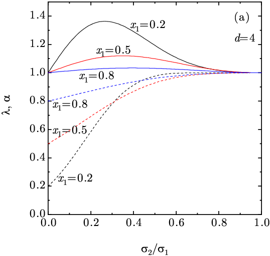
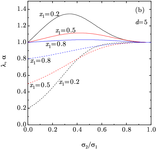
Figure 3 shows that $\lambda>1$ , while $\alpha<1$ , except if the mole fraction of the big spheres is large enough (not shown). According to Equations (22) and (25), this implies that (i) $\eta_{\text{eff}}<\eta$ and (ii) the surplus pressure of the mixture at a packing fraction $\eta$ is generally smaller than that of the monocomponent fluid at the equivalent packing fraction $\eta_{\text{eff}}$ . It is also worthwhile noting that, in contrast to what happens with $\bar{B}_{2}$ and $\bar{B}_{3}$ (see Figure 1), $\lambda$ has a nonmonotonic dependence on the size ratio and $\alpha$ also exhibits a nonmonotonic behavior if $x_{1}$ is small enough.

While we have proved the sp approach to be successful for both hard-disk ( $d=2$ ) Santos et al. 2017 and hard-sphere ( $d=3$ ) Santos et al. 2014 mixtures, one of our goals is to test it for $d=4$ and $d=5$ as well.

3 Comparison with Computer Simulation Results

In order to obtain explicit numerical results for the different approximations to the EOS of four- and five-dimensional hard-sphere mixtures, we require an expression for $Z_{\text{s}}(\eta)$ . While other choices are available, we considered here the empirical proposal that works for both dimensionalities by Luban and Michels (LM) Luban and Michels 1990, which reads

Z_{\text{s}}(\eta)=1+b_{2}\eta\frac{1+\left[b_{3}/b_{2}-\zeta(\eta)b_{4}/b_{3}\right]\eta}{1-\zeta(\eta)(b_{4}/b_{3})\eta+\left[\zeta(\eta)-1\right](b_{4}/b_{2})\eta^{2}},

(26)

where $\zeta(\eta)=\zeta_{0}+\zeta_{1}\eta/\eta_{\text{cp}}$ , $\eta_{\text{cp}}$ being the crystalline close-packing value. The values of $b_{2}$ , $b_{3}$ , $b_{4}$ , $\zeta_{0}$ , $\zeta_{1}$ , and $\eta_{\text{cp}}$ are given in Table 1.

Table 1: Values of

b_{2}

–

b_{4}

\zeta_{0}

\zeta_{1}

, and

\eta_{\text{cp}}

for

d=4

and

5

	$d=4$	$d=5$
$b_{2}$	$8$	$16$
$b_{3}$	$2^{6}\left(\frac{4}{3}-\frac{3\sqrt{3}}{2\pi}\right)\simeq 32.406$	$106$
$b_{4}$	$2^{9}\left(2-\frac{27\sqrt{3}}{4\pi}+\frac{832}{45\pi^{2}}\right)\simeq 77.7452$	$\frac{25\,315\,393}{8\,008}+\frac{3\,888\,425\sqrt{2}}{4\,004\pi}-\frac{67\,183\,425\arccos(1/3)}{8\,008\pi}\simeq 311.183$
$\zeta_{0}$	$1.2973(59)$	$1.074(16)$
$\zeta_{1}$	$-0.062(13)$	$0.163(45)$
$\eta_{\text{cp}}$	$\frac{\pi^{2}}{16}\simeq 0.617$	$\frac{\pi^{2}\sqrt{2}}{30}\simeq 0.465$

In Table 2 we list the systems whose compressibility factor has been obtained from simulation, either using MD González-Melchor et al. 2001 or MC Bishop and Whitlock 2012; Bishop and Whitlock 2016 methods. The values of the corresponding coefficients $\bar{B}_{2}$ [see Equation (9)], $\bar{B}_{3}$ [see Equations (16)–(18)], $\lambda$ , and $\alpha$ [see Equation (23)] are also included. We assigned a three-character label to each system, where the first (capital) letter denotes the size ratio (A–F for $\sigma_{2}/\sigma_{1}=\frac{1}{4}$ , $\frac{1}{3}$ , $\frac{2}{5}$ , $\frac{1}{2}$ , $\frac{3}{5}$ , and $\frac{3}{4}$ , respectively), the second (lower-case) letter denotes the mole fraction (a, b, and c for $x_{1}=0.25$ , $0.50$ , and $0.75$ , respectively), and the digit ( $4$ or $5$ ) denotes the dimensionality.

Table 2: Binary mixtures of four- and five-dimensional hard spheres studied through simulations (Monte Carlo—MC or molecular dynamics—MD) and the values of their coefficients

\bar{B}_{2}

[see Equation (9)],

\bar{B}_{3}

[see Equations (16)–(18)],

\lambda

, and

\alpha

[see Equation (23)].

$d$	Label	$\sigma_{2}/\sigma_{1}$	$x_{1}$	Simulation method	$\bar{B}_{2}$	$\bar{B}_{3}$	$\lambda$	$\alpha$
$4$	Aa4	${1}/{4}$	$0.25$	MD ¹¹footnotemark: 1	$3.85618$	$12.2253$	$1.28824$	$0.677138$
	Ab4	${1}/{4}$	$0.50$	MD ¹¹footnotemark: 1	$5.21595$	$18.8828$	$1.10923$	$0.741033$
	Ac4	${1}/{4}$	$0.75$	MD ¹¹footnotemark: 1	$6.60436$	$25.6326$	$1.03810$	$0.862800$
	Ba4	${1}/{3}$	$0.25$	MD ¹¹footnotemark: 1	$4.42857$	$14.4931$	$1.28470$	$0.808392$
	Bb4	${1}/{3}$	$0.50$	MD ¹¹footnotemark: 1	$5.56098$	$20.2530$	$1.11943$	$0.816497$
	Bc4	${1}/{3}$	$0.75$	MD ¹¹footnotemark: 1	$6.77049$	$26.2935$	$1.04334$	$0.897356$
	Cb4	${2}/{5}$	$0.50$	MC ²²footnotemark: 2	$5.87285$	$21.5939$	$1.11692$	$0.868418$
	Da4	${1}/{2}$	$0.25$	MD ¹¹footnotemark: 1	$5.82895$	$20.8444$	$1.17876$	$0.958523$
	Db4	${1}/{2}$	$0.50$	MD ¹¹footnotemark: 1 and MC ²²footnotemark: 2	$6.38235$	$23.9444$	$1.09883$	$0.928396$
	Dc4	${1}/{2}$	$0.75$	MD ¹¹footnotemark: 1	$7.15816$	$28.0333$	$1.04047$	$0.952376$
	Eb4	${3}/{5}$	$0.50$	MC ²²footnotemark: 2	$6.90085$	$26.5045$	$1.07078$	$0.966532$
	Fa4	${3}/{4}$	$0.25$	MD ¹¹footnotemark: 1	$7.55661$	$29.9061$	$1.03231$	$0.998173$
	Fb4	${3}/{4}$	$0.50$	MD ¹¹footnotemark: 1	$7.56231$	$29.9832$	$1.02894$	$0.992515$
	Fc4	${3}/{4}$	$0.75$	MD ¹¹footnotemark: 1	$7.73940$	$30.9790$	$1.01561$	$0.993060$
$5$	Aa5	${1}/{4}$	$0.25$	MD ¹¹footnotemark: 1	$6.30550$	$32.9426$	$1.24358$	$0.546995$
	Ab5	${1}/{4}$	$0.50$	MD ¹¹footnotemark: 1	$9.52439$	$57.2455$	$1.08739$	$0.671954$
	Ac5	${1}/{4}$	$0.75$	MD ¹¹footnotemark: 1	$12.7601$	$81.6145$	$1.02988$	$0.831562$
	Ba5	${1}/{3}$	$0.25$	MD ¹¹footnotemark: 1	$7.21951$	$37.7995$	$1.27656$	$0.675687$
	Bb5	${1}/{3}$	$0.50$	MD ¹¹footnotemark: 1	$10.0984$	$60.3097$	$1.10651$	$0.742645$
	Bc5	${1}/{3}$	$0.75$	MD ¹¹footnotemark: 1	$13.0411$	$83.1175$	$1.03739$	$0.863898$
	Cb5	${2}/{5}$	$0.50$	MC ³³footnotemark: 3 ^,4	$10.6565$	$63.6666$	$1.11369$	$0.798464$
	Da5	${1}/{2}$	$0.25$	MD ¹¹footnotemark: 1	$9.89286$	$55.1378$	$1.22316$	$0.886983$
	Db5	${1}/{2}$	$0.50$	MD ¹¹footnotemark: 1 and MC ³³footnotemark: 3 ^,5	$11.6818$	$70.5615$	$1.10812$	$0.874437$
	Dc5	${1}/{2}$	$0.75$	MD ¹¹footnotemark: 1	$13.7964$	$88.0120$	$1.04172$	$0.925768$
	Fa5	${3}/{4}$	$0.25$	MD ¹¹footnotemark: 1	$14.5176$	$92.4875$	$1.04866$	$0.990981$
	Fb5	${3}/{4}$	$0.50$	MD ¹¹footnotemark: 1	$14.6327$	$93.8346$	$1.03957$	$0.982162$
	Fc5	${3}/{4}$	$0.75$	MD ¹¹footnotemark: 1	$15.2162$	$99.1168$	$1.02005$	$0.986104$

¹ Ref. González-Melchor et al. 2001, ² Ref. Bishop and Whitlock 2012, ³ Ref. Bishop and Whitlock 2016, ⁴

x_{1}=\frac{971}{1944}=0.499486

, ⁵

x_{1}=\frac{973}{1944}=0.500514

If, as before, the degree of bidispersity is measured by $1-\bar{B}_{2}/b_{2}$ and $1-\bar{B}_{3}/b_{3}$ , we can observe the following ordering of decreasing bidispersity in the four-dimensional systems: Aa, Ba, Ab, Bb, Da, Cb, Db, Ac, Bc, Eb, Dc, Fa, Fb, and Fc. The same ordering applies in the case of the five-dimensional systems, except that, apart from the absence of the system Eb, the sequence {Ab, Bb, Da} is replaced by either {Ab, Da, Bb} or by {Da, Ab, Bb} if either $1-\bar{B}_{2}/b_{2}$ or $1-\bar{B}_{3}/b_{3}$ are used, respectively.

It should be stressed that the proposals implied by Equations (4), (13), (19), (20), and (25) may be interpreted in two directions. On the one hand, if $Z_{\text{s}}$ is known as a function of the packing fraction, then one can readily compute the compressibility factor of the mixture for any packing fraction and composition [ $\eta_{\text{eff}}$ and $\eta$ being related through Equation (22) in the case of $Z_{\text{sp}}$ ]; this is the standard view. On the other hand, if simulation data for the EOS of the mixture are available for different densities, size ratios, and mole fractions, Equations (4), (13), (19), (20), and (25) can be used to infer the compressibility factor of the monocomponent fluid. This is particularly important in the high-density region, where obtaining data from simulation may be accessible in the case of mixtures but either difficult or not feasible in the case of the monocomponent fluid, as happens in the metastable fluid branch Santos et al. 2017; Santos et al. 2014.

In principle, simulation data for different mixtures would yield different inferred functions $Z_{\text{s}}(\eta)$ . Thus, without having to use an externally imposed monocomponent EOS, the degree of collapse of the mapping from mixture compressibility factors onto a common function $Z_{\text{s}}(\eta)$ is an efficient way of assessing the performance of Equations (4), (13), (19), (20), and (25). As shown in Figure 4, the usefulness of those mappings is confirmed by the nice collapse obtained for all the points corresponding to the mixtures described in Table 2. The inferred data associated with $Z_{\text{\={e}2}}$ are almost identical to those associated with $Z_{\text{e2}}$ and thus they are omitted in Figure 4. Figure 4 also shows that the inferred curves are very close to the LM (monocomponent) EOS, Equation (26), what validates its choice as an accurate function $Z_{\text{s}}(\eta)$ in what follows. Notwithstanding this, one can observe in the high-density regime that the values inferred from simulation data via $Z_{\text{e1}}$ and $Z_{\text{\={e}1}}$ tend to underestimate the LM curve for both $d=4$ and $d=5$ , while the values inferred via $Z_{\text{e2}}$ tend to overestimate it for $d=5$ . Overall, one can say that the best agreement with the LM EOS is obtained by using $Z_{\text{e2}}$ and $Z_{\text{sp}}$ for $d=4$ and $d=5$ , respectively.

Now we turn to a more a direct comparison between the simulation data and the approximate EOS for mixtures. As expected from the indirect representation of Figure 4, we observed a very good agreement (not shown) between the simulation data for the systems displayed in Table 2 and the theoretical predictions obtained from Equations (4), (13), (19), (20), and (25), supplemented by Equation (26).

In order to perform a more stringent assessment of the five theoretical EOS, we chose $Z_{\text{e1}}(\eta)$ as a reference theory and focused on the percentage deviation $100[Z(\eta)/Z_{\text{e1}}(\eta)-1]$ from it. The results are displayed in Figures 5 and 7 for $d=4$ and Figures 8 and 9 for $d=5$ . Those figures reinforce the view that all our theoretical proposals are rather accurate: the errors in $Z_{\text{e1}}$ were typically smaller than $1$ % and they are even smaller in the other approximate EOS. Note that we have not put error bars in the MD data since they were unfortunately not reported in Reference González-Melchor et al. 2001. We must also mention that the MD data were generally more scattered than the MC ones. Moreover, certain (small) discrepancies between MC and MD points can be observed in Figure 7c, MC data generally lying below MD data. The same feature is also present (although somewhat less apparent) in Figure 9c. This may be due to larger finite-size effects in the MD simulations than in the MC simulations: the MD simulations used $648$ hyperspheres for $d=4$ and $512$ or $1024$ hyperspheres for $d=5$ , while the MC simulations used 10,000 hyperspheres for $d=4$ and 3888 or 7776 for $d=5$ . In any case, since the MC data were statistically precise, the discrepancy might be eliminated by the inclusion of the (unknown) error bars in the MD results. It is also worth pointing out that the representation of Figures 5–9 is much more demanding than a conventional representation of $Z$ vs $\eta$ for each mixture or even the representation of Figure 4.

4 Discussion and Concluding Remarks

In this paper we have carried out a thorough comparison between our theoretical proposals for the EOS of a multicomponent $d$ -dimensional mixture of hard hyperspheres and the available simulation results for binary mixtures of both four- and five-dimensional hard hyperspheres. It should be stressed that in this comparison we have restricted ourselves to the liquid branch. Let us now summarize the outcome of the different theories for the compressibility factor.

First, we note that $Z_{\text{\={e}2}}(\eta)\approx Z_{\text{e2}}(\eta)<Z_{\text{sp}}(\eta)<Z_{\text{\={e}1}}(\eta)<Z_{\text{e1}}(\eta)$ . The fact that $Z_{\text{\={e}2}}(\eta)\approx Z_{\text{e2}}(\eta)$ is a consequence of the small deviations of $B_{3}^{\text{e2}}$ from the exact third virial coefficient (see Figure 2). Thus, there does not seem to be any practical advantage in choosing $Z_{\text{\={e}2}}$ instead of $Z_{\text{e2}}$ , especially if $d=4$ [where the exact $B_{3}$ has a rather involved expression, see Equations (18)]. If one restricts oneself to the comparison between those approximate EOS that do not yield the exact $B_{3}$ , namely $Z_{\text{e1}}$ and $Z_{\text{e2}}$ , we find that $Z_{\text{e2}}$ performs generally better. On the other hand, if approximations requiring the exact $B_{3}$ as input are considered, namely $Z_{\text{\={e}1}}$ , $Z_{\text{\={e}2}}$ , and $Z_{\text{sp}}$ , the conclusion is that $Z_{\text{sp}}$ generally outperforms the other two.

The comparison with the simulation data confirms that the good agreement between the results of $Z_{\text{e1}}(\eta)$ that had been found earlier in connection with both MD González-Melchor et al. 2001 and MC Bishop and Whitlock 2012; Bishop and Whitlock 2016 simulation data are even improved by the other approximate theories. In fact, in both the four- and five-dimensional cases, the best agreement with the MD results is generally obtained from $Z_{\text{\={e}1}}$ and $Z_{\text{sp}}$ . On the other hand, for the four-dimensional case, the best agreement with the MC results corresponds to $Z_{\text{\={e}2}}\approx Z_{\text{e2}}$ , while that for the five-dimensional case corresponds to $Z_{\text{sp}}$ .

Finally, it must be pointed out that it seems that overall $Z_{\text{sp}}$ exhibits the best global behavior. However, more accurate simulation data would be needed to confirm this conclusion. It should also be stressed that the performance of the analyzed approximate EOS for fluid mixtures might be affected by the reliability of the (monocomponent) LM EOS. In any event, one may reasonably argue that the mapping between the compressibility factor of the mixture and the one of the monocomponent system with an effective packing fraction [see Equations (22) and (25)] that had already been tested in two- Santos et al. 2017 and three-dimensional Santos et al. 2014 mixtures is confirmed as an excellent approach also for higher dimensions.

Author Contributions

A.S. proposed the idea and the three authors performed the calculations. The three authors also participated in the analysis and discussion of the results and worked on the revision and writing of the final manuscript. All authors have read and agreed to the published version of the manuscript.

Funding

A.S. and S.B.Y. acknowledge financial support from the Spanish Agencia Estatal de Investigación through Grant No. FIS2016-76359-P and the Junta de Extremadura (Spain) through Grant No. GR18079, both partially financed by Fondo Europeo de Desarrollo Regional funds.

Conflicts of Interest

The authors declare no conflict of interest.

The following abbreviations are used in this manuscript:
EOS Equation of state LM Luban–Michels MC Monte Carlo MD Molecular dynamics

References

Frisch et al. (1985) Frisch, H.L.; Rivier, N.; Wyler, D. Classical Hard-Sphere Fluid in Infinitely Many Dimensions. Phys. Rev. Lett. 1985, 54, 2061–2063, doi:10.1103/PhysRevLett.54.2061.
Luban (1986) Luban, M. Comment on “Classical Hard-Sphere Fluid in Infinitely Many Dimensions”. Phys. Rev. Lett. 1986, 56, 2330–2330, doi:10.1103/PhysRevLett.56.2330.
Frisch et al. (1986) Frisch, H.L.; Rivier, N.; Wyler, D. Frisch, Rivier, and Wyler Respond. Phys. Rev. Lett. 1986, 56, 2331–2331, doi:10.1103/PhysRevLett.56.2331.
Klein and Frisch (1986) Klein, W.; Frisch, H.L. Instability in the infinite dimensional hard-sphere fluid. J. Chem. Phys. 1986, 84, 968–970, doi:10.1063/1.450544.
Wyler et al. (1987) Wyler, D.; Rivier, N.; Frisch, H.L. Hard-sphere fluid in infinite dimensions. Phys. Rev. A 1987, 36, 2422–2431, doi:10.1103/PhysRevA.36.2422.
Bagchi and Rice (1988) Bagchi, B.; Rice, S.A. On the stability of the infinite dimensional fluid of hard hyperspheres: A statistical mechanical estimate of the density of closest packing of simple hypercubic lattices in spaces of large dimensionality. J. Chem. Phys. 1988, 88, 1177–1184, doi:10.1063/1.454237.
Elskens and Frisch (1988) Elskens, Y.; Frisch, H.L. Kinetic theory of hard spheres in infinite dimensions. Phys. Rev. A 1988, 37, 4351–4353, doi:10.1103/PhysRevA.37.4351.
Carmesin et al. (1991) Carmesin, H.O.; Frisch, H.; Percus, J. Binary nonadditive hard-sphere mixtures at high dimension. J. Stat. Phys. 1991, 63, 791–795, doi:10.1007/BF01029212.
Frisch and Percus (1999) Frisch, H.L.; Percus, J.K. High dimensionality as an organizing device for classical fluids. Phys. Rev. E 1999, 60, 2942–2948, doi:10.1103/PhysRevE.60.2942.
Parisi and Slanina (2000) Parisi, G.; Slanina, F. Toy model for the mean-field theory of hard-sphere liquids. Phys. Rev. E 2000, 62, 6554–6559, doi:10.1103/PhysRevE.62.6554.
Yukhimets et al. (2000) Yukhimets, A.; Frisch, H.L.; Percus, J.K. Molecular Fluids at High Dimensionality. J. Stat. Phys. 2000, 100, 135–151, doi:10.1023/A:1018635527522.
Charbonneau et al. (2017) Charbonneau, P.; Kurchan, J.; Parisi, G.; Urbani, P.; Zamponi, F. Glass and Jamming Transitions: From Exact Results to Finite-Dimensional Descriptions. Annu. Rev. Cond. Matter Phys. 2017, 8, 265–288, doi:10.1146/annurev-conmatphys-031016-025334.
Santos and López de Haro (2005) Santos, A.; López de Haro, M. Demixing can occur in binary hard-sphere mixtures with negative non-additivity. Phys. Rev. E 2005, 72, 010501(R), doi:10.1103/PhysRevE.72.010501.
Freasier and Isbister (1981) Freasier, C.; Isbister, D.J. A remark on the Percus–Yevick approximation in high dimensions. Hard core systems. Mol. Phys. 1981, 42, 927–936, doi:10.1080/00268978100100711.
Leutheusser (1984) Leutheusser, E. Exact solution of the Percus–Yevick equation for a hard-core fluid in odd dimensions. Physica A 1984, 127, 667–676, doi:10.1016/0378-4371(84)90050-5.
Michels and Trappeniers (1984) Michels, J.P.J.; Trappeniers, N.J. Dynamical computer simulations on hard hyperspheres in four- and five-dimensional space. Phys. Lett. A 1984, 104, 425–429, doi:10.1016/0375-9601(84)90749-7.
Baus and Colot (1986) Baus, M.; Colot, J.L. Theoretical structure factors for hard-core fluids. J. Phys. C 1986, 19, L643–L648, doi:10.1088/0022-3719/19/28/002.
Baus and Colot (1987) Baus, M.; Colot, J.L. Thermodynamics and structure of a fluid of hard rods, disks, spheres, or hyperspheres from rescaled virial expansions. Phys. Rev. A 1987, 36, 3912–3925, doi:10.1103/PhysRevA.36.3912.
Rosenfeld (1987) Rosenfeld, Y. Distribution function of two cavities and Percus–Yevick direct correlation functions for a hard sphere fluid in $D$ dimensions: Overlap volume function representation. J. Chem. Phys. 1987, 87, 4865–4869, doi:10.1063/1.452797.
Rosenfeld (1988) Rosenfeld, Y. Scaled field particle theory of the structure and thermodynamics of isotropic hard particle fluids. J. Chem. Phys. 1988, 89, 4272–4287, doi:10.1063/1.454810.
Amorós et al. (1989) Amorós, J.; Solana, J.R.; Villar, E. Equations of state for four- and five-dimensional hard hypersphere fluids. Phys. Chem. Liq. 1989, 19, 119–124, doi:10.1080/00319108908028443.
Song et al. (1989) Song, Y.; Mason, E.A.; Stratt, R.M. Why does the Carnahan-Starling equation work so well? J. Phys. Chem. 1989, 93, 6916–6919, doi:10.1021/j100356a008.
Song and Mason (1990) Song, Y.; Mason, E.A. Equation of state for fluids of spherical particles in $d$ dimensions. J. Chem. Phys. 1990, 93, 686–688, doi:10.1063/1.459517.
González et al. (1990) González, D.J.; González, L.E.; Silbert, M. Thermodynamics of a fluid of hard $D$ -dimensional spheres: Percus-Yevick and Carnahan-Starling-like results for $D=4$ and $5$ . Phys. Chem. Liq. 1990, 22, 95–102, doi:10.1080/00319109008036415.
Luban and Michels (1990) Luban, M.; Michels, J.P.J. Equation of state of hard $D$ -dimensional hyperspheres. Phys. Rev. A 1990, 41, 6796–6804, doi:10.1103/PhysRevA.41.6796.
Maeso et al. (1991) Maeso, M.J.; Solana, J.R.; Amorós, J.; Villar, E. Equations of state for D-dimensional hard sphere fluids. Mater. Chem. Phys. 1991, 30, 39–42, doi:10.1016/0254-0584(91)90151-J.
González et al. (1991) González, D.J.; González, L.E.; Silbert, M. Structure and thermodynamics of hard $D$ -dimensional spheres: overlap volume function approach. Mol. Phys. 1991, 74, 613–627, doi:10.1080/00268979100102461.
González et al. (1992) González, L.E.; González, D.J.; Silbert, M. Structure and thermodynamics of mixtures of hard $D$ -dimensional spheres: Overlap volume function approach. J. Chem. Phys. 1992, 97, 5132–5141, doi:10.1063/1.463810.
Velasco et al. (1999) Velasco, E.; Mederos, L.; Navascués, G. Analytical approach to the thermodynamics and density distribution of crystalline phases of hard spheres spheres. Mol. Phys. 1999, 97, 1273–1277, doi:10.1080/00268979909482929.
Bishop et al. (1999) Bishop, M.; Masters, A.; Clarke, J.H.R. Equation of state of hard and Weeks–Chandle–Anderson hyperspheres in four and five dimensions. J. Chem. Phys. 1999, 110, 11449–11453, doi:10.1063/1.479086.
Finken et al. (2001) Finken, R.; Schmidt, M.; Löwen, H. Freezing transition of hard hyperspheres. Phys. Rev. E 2001, 65, 016108, doi:10.1103/PhysRevE.65.016108.
Santos et al. (1999) Santos, A.; Yuste, S.B.; López de Haro, M. Equation of state of a multicomponent $d$ -dimensional hard-sphere fluid. Mol. Phys. 1999, 96, 1–5, doi:10.1080/00268979909482932.
Mon and Percus (1999) Mon, K.K.; Percus, J.K. Virial expansion and liquid-vapor critical points of high dimension classical fluids. J. Chem. Phys. 1999, 110, 2734–2735, doi:10.1063/1.477998.
Santos (2000) Santos, A. An equation of state à La Carnahan-Starling A Five-Dimens. Fluid Hard Hyperspheres. J. Chem. Phys. 2000, 112, 10680–10681, doi:10.1063/1.481701.
Yuste et al. (2000) Yuste, S.B.; Santos, A.; López de Haro, M. Demixing in binary mixtures of hard hyperspheres. Europhys. Lett. 2000, 52, 158–164, doi:10.1209/epl/i2000-00411-9.
González-Melchor et al. (2001) González-Melchor, M.; Alejandre, J.; López de Haro, M. Equation of state and structure of binary mixtures of hard $d$ -dimensional hyperspheres. J. Chem. Phys. 2001, 114, 4905–4911, doi:10.1063/1.1349094.
Santos et al. (2002) Santos, A.; Yuste, S.B.; López de Haro, M. Contact values of the radial distribution functions of additive hard-sphere mixtures in $d$ dimensions: A new proposal. J. Chem. Phys. 2002, 117, 5785–5793, doi:10.1063/1.1502247.
Robles et al. (2004) Robles, M.; López de Haro, M.; Santos, A. Equation of state of a seven-dimensional hard-sphere fluid. Percus–Yevick theory and molecular-dynamics simulations. J. Chem. Phys. 2004, 120, 9113–9122, doi:10.1063/1.1701840.
Santos et al. (2005) Santos, A.; López de Haro, M.; Yuste, S.B. Equation of state of nonadditive $d$ -dimensional hard-sphere mixtures. J. Chem. Phys. 2005, 122, 024514, doi:10.1063/1.1832591.
Bishop et al. (2005) Bishop, M.; Whitlock, P.A.; Klein, D. The structure of hyperspherical fluids in various dimensions. J. Chem. Phys. 2005, 122, 074508, doi:10.1063/1.1848091.
Bishop and Whitlock (2005) Bishop, M.; Whitlock, P.A. The equation of state of hard hyperspheres in four and five dimensions. J. Chem. Phys. 2005, 123, 014507, doi:10.1063/1.1874793.
Lue and Bishop (2006) Lue, L.; Bishop, M. Molecular dynamics study of the thermodynamics and transport coefficients of hard hyperspheres in six and seven dimensions. Phys. Rev. E 2006, 74, 021201, doi:10.1103/PhysRevE.74.021201.
López de Haro et al. (2006) López de Haro, M.; Yuste, S.B.; Santos, A. Test of a universality ansatz for the contact values of the radial distribution functions of hard-sphere mixtures near a hard wall. Mol. Phys. 2006, 104, 3461–3467, doi:10.1080/00268970601028963.
Bishop and Whitlock (2007) Bishop, M.; Whitlock, P.A. Monte Carlo Simulation of Hard Hyperspheres in Six, Seven and Eight Dimensions for Low to Moderate Densities. J. Stat. Phys. 2007, 126, 299–314, doi:10.1007/s10955-006-9266-9.
Robles et al. (2007) Robles, M.; López de Haro, M.; Santos, A. Percus–Yevick theory for the structural properties of the seven-dimensional hard-sphere fluid. J. Chem. Phys. 2007, 126, 016101, doi:10.1063/1.2424459.
Whitlock et al. (2007) Whitlock, P.A.; Bishop, M.; Tiglias, J.L. Structure factor for hard hyperspheres in higher dimensions. J. Chem. Phys. 2007, 126, 224505, doi:10.1063/1.2743031.
Rohrmann and Santos (2007) Rohrmann, R.D.; Santos, A. Structure of hard-hypersphere fluids in odd dimensions. Phys. Rev. E 2007, 76, 051202, doi:10.1103/PhysRevE.76.051202.
López de Haro et al. (2008) López de Haro, M.; Yuste, S.B.; Santos, A. Alternative Approaches to the Equilibrium Properties of Hard-Sphere Liquids. In Theory and Simulation of Hard-Sphere Fluids and Related Systems; Mulero, A., Ed.; Lecture Notes in Physics; Springer: Berlin, Germany, 2008; Volume 753, pp. 183–245.
Bishop et al. (2008) Bishop, M.; Clisby, N.; Whitlock, P.A. The equation of state of hard hyperspheres in nine dimensions for low to moderate densities. J. Chem. Phys. 2008, 128, 034506, doi:10.1063/1.2821962.
Adda-Bedia et al. (2008) Adda-Bedia, M.; Katzav, E.; Vella, D. Solution of the Percus–Yevick equation for hard hyperspheres in even dimensions. J. Chem. Phys. 2008, 129, 144506, doi:10.1063/1.2991338.
Rohrmann et al. (2008) Rohrmann, R.D.; Robles, M.; López de Haro, M.; Santos, A. Virial series for fluids of hard hyperspheres in odd dimensions. J. Chem. Phys. 2008, 129, 014510, doi:10.1063/1.2951456.
van Meel et al. (2009) van Meel, J.A.; Charbonneau, B.; Fortini, A.; Charbonneau, P. Hard-sphere crystallization gets rarer with increasing dimension. Phys. Rev. E 2009, 80, 061110, doi:10.1103/PhysRevE.80.061110.
Lue et al. (2010) Lue, L.; Bishop, M.; Whitlock, P.A. The fluid to solid phase transition of hard hyperspheres in four and five dimensions. J. Chem. Phys. 2010, 132, 104509, doi:10.1063/1.3354115.
Rohrmann and Santos (2011) Rohrmann, R.D.; Santos, A. Multicomponent fluids of hard hyperspheres in odd dimensions. Phys. Rev. E 2011, 83, 011201, doi:10.1103/PhysRevE.83.011201.
Leithall and Schmidt (2011) Leithall, G.; Schmidt, M. Density functional for hard hyperspheres from a tensorial-diagrammatic series. Phys. Rev. E 2011, 83, 021201, doi:10.1103/PhysRevE.83.021201.
Estrada and Robles (2011) Estrada, C.D.; Robles, M. Fluid–solid transition in hard hypersphere systems. J. Chem. Phys. 2011, 134, 044115, doi:10.1063/1.3530780.
Bishop and Whitlock (2012) Bishop, M.; Whitlock, P.A. Monte Carlo study of four dimensional binary hard hypersphere mixtures. J. Chem. Phys. 2012, 136, 014506, doi:10.1063/1.3671651.
Bishop and Whitlock (2013) Bishop, M.; Whitlock, P.A. Phase transitions in four-dimensional binary hard hypersphere mixtures. J. Chem. Phys. 2013, 138, 084502, doi:10.1063/1.4789953.
Bishop and Whitlock (2016) Bishop, M.; Whitlock, P.A. Five dimensional binary hard hypersphere mixtures: A Monte Carlo study. J. Chem. Phys. 2016, 145, 154502, doi:10.1063/1.4964614.
Amorós and Ravi (2013) Amorós, J.; Ravi, S. On the application of the Carnahan–Starling method for hard hyperspheres in several dimensions. Phys. Lett. A 2013, 377, 2089–2092, doi:10.1016/j.physleta.2013.06.004.
Amorós (2014) Amorós, J. Equations of state for tetra-dimensional hard-sphere fluids. Phys. Chem. Liq. 2014, 52, 287–290, doi:10.1080/00319104.2013.820301.
Heinen et al. (2015) Heinen, M.; Horbach, J.; Löwen, H. Liquid pair correlations in four spatial dimensions: Theory versus simulation. Mol. Phys. 2015, 113, 1164–1169, doi:10.1080/00268976.2014.993736.
Santos (2016) Santos, A. A Concise Course on the Theory of Classical Liquids. Basics and Selected Topics; Lecture Notes in Physics; Springer: New York, NY, USA, 2016; Volume 923.
Santos et al. (2017) Santos, A.; Yuste, S.B.; López de Haro, M.; Ogarko, V. Equation of state of polydisperse hard-disk mixtures in the high-density regime. Phys. Rev. E 2017, 93, 062603, doi:10.1103/PhysRevE.062603.
Akhouri (2017) Akhouri, B.P. Equations of state for hard hypersphere fluids in high dimensional spaces. Int. J. Chem. Stud. 2017, 5, 39–45, doi:10.22271/chemi.
Ivanizki (2018) Ivanizki, D. A generalization of the Carnahan–Starling approach with applications to four- and five-dimensional hard spheres. Phys. Lett. A 2018, 382, 1745–1751, doi:10.1016/j.physleta.2018.04.036.
Santos et al. (2001) Santos, A.; Yuste, S.B.; López de Haro, M. Virial coefficients and equations of state for mixtures of hard discs, hard spheres, and hard hyperspheres. Mol. Phys. 2001, 99, 1959–1972, doi:10.1080/00268970110063890.
Ree and Hoover (1964) Ree, F.H.; Hoover, W.G. On the Signs of the Hard Sphere Virial Coefficients. J. Chem. Phys. 1964, 40, 2048–2049, doi:10.1063/1.1725456.
Luban and Baram (1982) Luban, M.; Baram, A. Third and fourth virial coefficients of hard hyperspheres of arbitrary dimensionality. J. Chem. Phys. 1982, 76, 3233–3241, doi:10.1063/1.443316.
Joslin (1982) Joslin, C.G. Third and fourth virial coefficients of hard hyperspheres of arbitrary dimensionality. J. Chem. Phys. 1982, 77, 2701–2702, doi:10.1063/1.444104.
Loeser et al. (1991) Loeser, J.G.; Zhen, Z.; Kais, S.; Herschbach, D.R. Dimensional interpolation of hard sphere virial coefficients. J. Chem. Phys. 1991, 95, 4525–4544, doi:10.1063/1.461776.
Enciso et al. (2002) Enciso, E.; Almarza, N.G.; González, M.A.; Bermejo, F.J. The virial coefficients of hard hypersphere binary mixtures. Mol. Phys. 2002, 100, 1941–1944, doi:10.1080/00268970110108322.
Bishop et al. (2004) Bishop, M.; Masters, A.; Vlasov, A.Y. Higher virial coefficients of four and five dimensional hard hyperspheres. J. Chem. Phys. 2004, 121, 6884–6886, doi:10.1063/1.1777574.
Clisby and McCoy (2004a) Clisby, N.; McCoy, B.M. Analytic Calculation of ${B_{4}}$ for Hard Spheres in Even Dimensions. J. Stat. Phys. 2004, 114, 1343–1360, doi:10.1023/B:JOSS.0000013959.30878.d2.
Clisby and McCoy (2004b) Clisby, N.; McCoy, B. Negative Virial Coefficients and the Dominance of Loose Packed Diagrams for $D$ -Dimensional Hard Spheres. J. Stat. Phys. 2004, 114, 1361–1392, doi:10.1023/B:JOSS.0000013960.83555.7d.
Bishop et al. (2005) Bishop, M.; Masters, A.; Vlasov, A.Y. The eighth virial coefficient of four- and five-dimensional hard hyperspheres. J. Chem. Phys. 2005, 122, 154502, doi:10.1063/1.1882273.
Clisby and McCoy (2005) Clisby, N.; McCoy, B.M. New results for virial coeffcients of hard spheres in ${D}$ dimensions. Pramana 2005, 64, 775–783, doi:10.1007/BF02704582.
Lyberg (2005) Lyberg, I. The fourth virial coefficient of a fluid of hard spheres in odd dimensions. J. Stat. Phys. 2005, 119, 747–764, doi:10.1007/s10955-005-3020-6.
Clisby and McCoy (2006) Clisby, N.; McCoy, B.M. Ninth and Tenth Order Virial Coefficients for Hard Spheres in ${D}$ Dimensions. J. Stat. Phys. 2006, 122, 15–57, doi:10.1007/s10955-005-8080-0.
Zhang and Pettitt (2016) Zhang, C.; Pettitt, B.M. Computation of high-order virial coefficients in high-dimensional hard-sphere fluids by Mayer sampling. Mol. Phys. 2016, 112, 1427–1447, doi:10.1080/00268976.2014.904945.
Skoge et al. (2006) Skoge, M.; Donev, A.; Stillinger, F.H.; Torquato, S. Packing Hyperspheres in high-dimensional Euclidean spaces. Phys. Rev. E 2006, 74, 041127, doi:10.1103/PhysRevE.74.041127.
Torquato and Stillinger (2006a) Torquato, S.; Stillinger, F.H. New Conjectural Lower Bounds on the Optimal Density of Sphere Packings. Exp. Math. 2006, 15, 307–331, doi:10.1080/10586458.2006.10128964.
Torquato and Stillinger (2006b) Torquato, S.; Stillinger, F.H. Exactly Solvable Disordered Hard-Sphere Packing Model in Arbitrary-Dimensional Euclidean Spaces. Phys. Rev. E 2006, 73, 031106, doi:10.1103/PhysRevE.73.031106.
Torquato et al. (2006) Torquato, S.; Uche, O.U.; Stillinger, F.H. Random sequential addition of hard spheres in high Euclidean dimensions. Phys. Rev. E 2006, 74, 061308, doi:10.1103/PhysRevE.74.061308.
Parisi and Zamponi (2006) Parisi, G.; Zamponi, F. Amorphous packings of hard spheres for large space dimension. J. Stat. Mech. 2006, P03017, doi:10.1088/1742-5468/2006/03/p03017.
Scardicchio et al. (2008) Scardicchio, A.; Stillinger, F.H.; Torquato, S. Estimates of the optimal density of sphere packings in high dimensions. J. Math. Phys. 2008, 49, 043301, doi:10.1063/1.2897027.
van Meel et al. (2009) van Meel, J.A.; Frenkel, D.; Charbonneau, P. Geometrical frustration: A study of four-dimensional hard spheres. Phys. Rev. E 2009, 79, 030201(R), doi:10.1103/PhysRevE.79.030201.
Agapie and Whitlock (2010) Agapie, S.C.; Whitlock, P.A. Random packing of hyperspheres and Marsaglia’s parking lot test. Monte Carlo Methods Appl. 2010, 16, 197–209, doi:10.1515/mcma.2010.019.
Torquato and Stillinger (2010) Torquato, S.; Stillinger, F.H. Jammed hard-particle packings: From Kepler to Bernal and beyond. Rev. Mod. Phys. 2010, 82, 2633–2672, doi:10.1103/RevModPhys.82.2633.
Zhang and Torquato (2013) Zhang, G.; Torquato, S. Precise algorithm to generate random sequential addition of hard hyperspheres at saturation. Phys. Rev. E 2013, 88, 053312, doi:10.1103/PhysRevE.88.053312.
Kazav et al. (2019) Kazav, E.; Berdichevsky, R.; Schwartz, M. Random close packing from hard-sphere Percus-Yevick theory. Phys. Rev. E 2019, 99, 012146, doi:10.1103/PhysRevE.99.012146.
Berthier et al. (2019) Berthier, L.; Charbonneau, P.; Kundu, J. Bypassing sluggishness: SWAP algorithm and glassiness in high dimensions. Phys. Rev. E 2019, 99, 031301(R), doi:10.1103/PhysRevE.99.031301.
Santos et al. (2014) Santos, A.; Yuste, S.B.; López de Haro, M.; Odriozola, G.; Ogarko, V. Simple effective rule to estimate the jamming packing fraction of polydisperse hard spheres. Phys. Rev. E 2014, 89, 040302(R), doi:10.1103/PhysRevE.89.040302.
Bishop et al. (1985) Bishop, M.; Michels, J.P.J.; de Schepper, I.M. The short-time behavior of the velocity autocorrelation function of smooth, hard hyperspheres in three, four and five dimensions. Phys. Lett. A 1985, 111, 169–170, doi:10.1016/0375-9601(85)90568-7.
Colot and Baus (1986) Colot, J.L.; Baus, M. The freezing of hard disks and hyperspheres. Phys. Lett. A 1986, 119, 135–139, doi:10.1016/0375-9601(86)90432-9.
Lue (2005) Lue, L. Collision statistics, thermodynamics, and transport coefficients of hard hyperspheres in three, four, and five dimensions. J. Chem. Phys. 2005, 122, 044513, doi:10.1063/1.1834498.
Santos (2012a) Santos, A. Note: An exact scaling relation for truncatable free energies of polydisperse hard-sphere mixtures. J. Chem. Phys. 2012, 136, 136102, doi:10.1063/1.3702439.
Santos (2012b) Santos, A. Class of consistent fundamental-measure free energies for hard-sphere mixtures. Phys. Rev. E 2012, 86, 040102(R), doi:10.1103/PhysRevE.86.040102.