Hysteretic Mutual Synchronization of PERP-STNO Pairs Analyzed by a Generalized Pendulum-like ModelPreprint: APS/123-QED

For a two-dimensional auto-oscillator, the stability is a vital and fundamental issue, from which one can find out the physical conditions to maintain persistent oscillatory states qualitatively and quantitatively. For this reason, we need to develop a new theoretical viewpoint and approach that is independent of coordinate system in order to determine the stability of two-dimensional auto-oscillators in a more straightforward way. Another reason we develop this new approach is to quantitatively estimate the perturbation level of auto-oscillatory trajectories caused by weak interactions among multiple auto-oscillators, and therefore obtain the equations of the phase angle dynamics for multiple coupled auto-oscillators (see Appendix A). This cannot be directly achieved from the approach based on the energy-averaging techniqueMayergoyz et al. 2009.

The general vector form for a two-dimensional autonomous system can be expressed as Mayergoyz et al. 2009

Here, $\mathbf{x}$ indicates the state vector of the system on a two dimensional phase plane. According to the Helmholz decomposition theoremMayergoyz et al. 2009, the tangent vector field $\textbf{f}(\textbf{x})$ on the phase plane can be uniquely decomposed into two components: one is the divergence free term $\textbf{f}_{\mathrm{d}}(\textbf{x})=(-\nabla_{\mathbf{x}}E_{0})\times\mathbf{n}$; the other is curl free term $\textbf{f}_{\mathrm{c}}(\textbf{x})=-\nabla_{\mathbf{x}}\Omega$. Here, $E_{0}(\mathbf{x})$, $\Omega(\mathbf{x})$, and $\mathbf{n}$ are scalar potentials and the unit vector normal to the plane, respectively. Furthermore, according to the balance equation of $E_{0}(\mathbf{x})$, only the component of $\textbf{f}_{\mathrm{c}}(\textbf{x})$ normal to $\textbf{f}_{\mathrm{d}}(\textbf{x})$ can contribute to the time rate of $E_{0}(\mathbf{x})$. Also, if $E_{0}(\mathbf{x})$ and $\textbf{f}_{\mathrm{c}}(\textbf{x})$ can be treated as energy and damping terms, respectively, then the component of $\textbf{f}_{\mathrm{c}}(\textbf{x})$ along $\textbf{f}_{\mathrm{d}}(\textbf{x})$ is sufficiently weak to hardly affect the oscillatory states governed by $\textbf{f}_{\mathrm{d}}(\textbf{x})$ through microscopic interactions with the environment. Thus, it is quite reasonable to assume $\textbf{f}_{\mathrm{d}}(\textbf{x})$ and $\textbf{f}_{\mathrm{c}}(\textbf{x})$ are normal to each other everywhere on the phase planeMayergoyz et al. 2009, that is, $\textbf{f}_{\mathrm{c}}(\mathbf{x})\approx-\Gamma(\mathbf{x})\nabla_{\mathbf{x}}E_{0}$. Here, $\Gamma(\mathbf{x})$ is the damping rate, which contains the positive and negative damping effects.

Therefore, Eq. (1) can be further written as

The first term on the right side of Eq. (2) defines a group of energy conserved trajectories(states) $C(E_{0})$ designated by $E_{0}$, implying that the effective particle is moving along the direction normal to $-\nabla_{\mathbf{x}}E_{0}(\mathbf{x})$. Besides, the first and second expressions in Eq. (2) are both equivalent. The damping term in the second expression is derived from the Rayleigh dissipation function. The unit vector $\mathbf{p}\equiv\nabla_{\mathbf{x}}E_{0}/|\nabla_{\mathbf{x}}E_{0}|$ is normal to the conservative trajectories. In the second expression, the non-conservative part contains two terms: first one is the positive damping term with a positive damping factor $\alpha(\mathbf{x})>0$; second one is the negative damping term with a negative damping factor $a(\mathbf{x},\mu)$, in which $\mu$ is used to adjust its intensity.

Actually, Eq. (2) can also be equivalently expressed in the viewpoint of force/fieldThiele 1973:

The left-hand side of Eq. (3) describes the gyro-force/field. The three forces/fields on the right side of Eq. (3) are given in turn as: restoring force/field $\mathbf{F}_{\mathrm{re}}(\mathbf{x})=-\nabla_{\mathbf{x}}E_{0}$ ; positive damping force/field $\mathbf{F}_{\mathrm{pd}}(\mathbf{x})=-\alpha(\mathbf{x})(d\mathbf{x}/dt)$; negative damping force/field $\mathbf{F}_{\mathrm{nd}}(\mathbf{x})=a(\mathbf{x},\mu)(\mathbf{p}\times\mathbf{n})$. As illustrated in Fig. 1 (a) and (b), when $\mathbf{F}_{\mathrm{pd}}(\mathbf{x})$ and $\mathbf{F}_{\mathrm{nd}}(\mathbf{x})$ compensate for each other, the dynamic states satisfying $\partial E_{0}/\partial p\neq 0$ (see Fig. 1(b)) can be driven by $\mathbf{F}_{\mathrm{nd}}(\mathbf{x,\mu})$. Here, the state vector can be expressed as $\mathbf{x}=p(\mathbf{x})\mathbf{p}+\phi(\mathbf{x})\mathbf{\hat{\phi}}$, and $\mathbf{\hat{\phi}}\equiv\mathbf{n}\times\mathbf{p}$.

As illustrated in Fig. 1, to confirm the stability of the dynamic states, one can use the following transformation to ensure that the moving effective particle is stationary in the new frame:

Here, the abbreviations ”N” and ”O” denote the new and old frames, respectively. Besides, $v_{p}(\mathbf{x})$ is a scalar velocity field, so here Eq. (4) is termed as a local coordinate transformation. By using Eq. (4), there are two new forces/fields induced in the new frame (see Fig. 1(c)): one is the fictitious force/field $\mathbf{F}_{\mathrm{fi}}(\mathbf{x})=-v_{p}(\mathbf{x})\mathbf{p}$; the other is the anti-negative damping force/field $\mathbf{F}_{\mathrm{and}}(\mathbf{x})=-\alpha(\mathbf{x})v_{p}(\mathbf{x})(\mathbf{p}\times\mathbf{n})$. If $\mathbf{v}_{p}$ is chosen so that $\mathbf{F}_{\mathrm{and}}$ cancels $\mathbf{F}_{\mathrm{nd}}$ on the phase plane, Eq. (3) will take the following form in the new frame:

Here, $\mathbf{F}_{\mathrm{N,re}}(\mathbf{x})=-\nabla_{\mathbf{x}}E_{N}$, $E_{N}(\mathbf{x})=E_{0}(\mathbf{x})+U^{\prime}_{N}(\mathbf{x})$, and $U^{\prime}_{N}(\mathbf{x})\equiv\int^{\mathbf{x}}d\mathbf{x}^{\prime}\cdot[v_{p}(\mathbf{x}^{\prime})\mathbf{p}]$. Also, $\mathbf{F}_{\mathrm{N,pd}}(\mathbf{x})=-\alpha(\mathbf{x})(d\mathbf{x}/dt)_{\mathrm{N}}$, and $\alpha(\mathbf{x})v_{p}(\mathbf{x})=a(\mathbf{x},\mu)$ has been utilized.

In principle, for stable auto-oscillatory states, the contour of $E_{N}$ exhibits canyon-like shapes, i.e. stable limit cycles. At anywhere on the bottom of the canyon, the values of $E_{N}$ are all equal, implying that the effective particle can be static at anywhere on the bottom of the canyon. For these canyons, one can determine them by walking along $\mathbf{p}_{N}=\nabla_{\mathbf{x}}E_{N}/|\nabla_{\mathbf{x}}E_{N}|$. And then, since the state vector in the new frame can be expanded as $\mathbf{x}=p_{N}(\mathbf{x})\mathbf{p}_{N}+\phi_{N}(\mathbf{x})\mathbf{\hat{\phi}}_{N}$, where $\mathbf{\hat{\phi}}_{N}\equiv\mathbf{n}\times\mathbf{p}_{N}$, $E_{N}$ must be only a function of $p_{N}(\mathbf{x})$. Thus, by requiring $(\partial E_{N}/\partial P_{N})_{P_{N0}}=0$ as well as $(\partial^{2}E_{N}/\partial P_{N}^{2})_{P_{N0}}>0$, we can find out the positions of these canyons and confirm their stability exactly, as illustrated in Fig. 1(d).

Strictly speaking, because $\mathbf{v}_{p}(\mathbf{x})$ in Eq. (4) depends not only on $p$ but also on $\phi$ (see also Appendix A.1), the actual auto-oscillatory trajectories, which are the meta-stable states of $E_{N}(\mathbf{x})$, are not exactly the same as the dynamic ones of $E_{0}(\mathbf{x})$, as illustrated in Figs. 1 (a) and (c). However, for most cases of auto-oscillators, due to the much larger order of $|\mathbf{F}_{\mathrm{re}}(\mathbf{x})|$ than those of $|\mathbf{F}_{\mathrm{pd}}(\mathbf{x})|$ and $|\mathbf{F}_{\mathrm{nd}}(\mathbf{x},\mu)|$, the auto-oscillations can be roughly treated as the dynamic states of $E_{0}(\mathbf{x})$, that is, $p_{N}(\mathbf{x})\approx p(\mathbf{x})$.

In the following, we take two simple examples, namely PERP-STNOsChen et al. 2019 and PMA-STNOsTaniguchi et al. 2013, to briefly introduce the practical usage of this new theory in analyzing the stability of STNOs. First, since these two types of STNOs both have axial symmetric anisotropic energies, their dynamic states (out-of-plane (OP) precessions) can both be designated by the z-component of the magnetization, i.e. $m_{z}$. Subsequently, their the dynamic state energies can be expressed as $E_{0}=(-k/2)m^{2}_{z}$, where $k<0$ in PERP-STNOs and $k>0$ in PMA-STNOs. Interestingly, notice that in PERP-STNOs the dynamic state energy has a positive curvature $\partial^{2}E_{0}/\partial m_{z}^{2}=-k>0$; while in PMA-STNOs the curvature is negative, $\partial^{2}E_{0}/\partial m_{z}^{2}=-k<0$. From the viewpoint of $E_{N}(m_{z})$, this implies that the dynamic state energy of PERP-STNOs itself possesses the potential to produce the stability of OP precessions. The effective energy $U^{\prime}_{N}(m_{z})$ produced by the STT was proven to just shift the equilibrium OP precessional point $m_{z0}$ away from the film plane, instead of changing the curvature of $E_{0}(m_{z})$ (see Ref.Chen et al. 2019). Thus, PERP-STNOs can be excited solely by currents with opposite injection directions without the assistance of an external magnetic field.

However, in PMA-STNOs we need a different type of STT. It has been proven that this can be provided by an in-plane polarizer with an asymmetric spin polarization factor, in order to turn the negative curvature of $E_{0}$ into a positive one of $E_{N}(m_{z})$(see Ref.Taniguchi et al. 2013). Thereby, PMA-STNOs can be excited only by positive current. Notably, due to the non-axially symmetric polarizer in PMA-STNOs, one can calculate $U^{\prime}_{N}(m_{z})$ by using the approach introduced in Appendix A.1. Furthermore, since the STT fails to shift the equilibrium point $m_{z0}$ of the OP state in PMA-STNOs, it is necessary to apply an external field along the z-axis to shift $m_{z0}$ away from the film plane. Here, the zeeman energy produced by the external field does not change the curvature of $E_{N}(m_{z0})$.

From the brief analyses above, we can conclude that for different types of two-dimensional dynamic state energies, the physical conditions to excite auto-oscillatory states are also different. In principle, all types of dynamic state energies have the potential to excite auto-oscillatory states, including (anti-)ferromagnetic exchange coupling, shape anisotropic energy, perpendicular magnetic anisotropic energy, zeeman energy, etc. However, in nature there are only a limited number of negative damping forces that exist, e.g. STT, and so dynamic states of some type do not remain stable. Finally, due to the positive curvature of $E_{N}(\mathrm{x})$ for all types of stable auto-oscillatory states, one can straightforwardly obtain the governing equation of phase angle for coupled multiple oscillators, as described in the following section.

For auto-oscillators with a strong nonlinear frequency shift coefficient $(\partial^{2}E_{0}/\partial p^{2})_{p_{0}}$ (see Fig. 1(b)as an example), the dynamics of phase angle $\phi$ will be coupled with that of momentum $p$Slavin and Tiberkevich 2009; Zhou et al. 2010, as detailed in the Appendix A.2. Based on this finding, the generalized pendulum-like particles for coupled auto-oscillators by weak interactions can be straightforwardly derived through the local coordinate transformation as (see Appendix A.2):

where $\alpha_{\mathrm{eff},i}(p_{i0})\equiv\alpha_{i}S_{i}(p_{i0})H^{(2)}_{N,i0}(p_{i0})$ and $F_{\mathrm{eff},i}(p_{i0})\equiv H_{N,i0}^{(2)}(p_{i0})a_{i}(p_{i0},\mu)$ are the effective damping constants and effective driving forces, respectively. Also, $H^{(2)}_{N,i0}(p_{i0})$, $S_{i}(p_{i0})$, $a_{i}(p_{i0},\mu_{i})$, and $H^{(2)}_{Oi}(p_{i0})$ are the stability, positive damping function, negative damping function, and nonlinear frequency shift coefficient Slavin and Tiberkevich 2009 of auto-oscillators, respectively, which are defined in Appendix A.2. $p_{i0}$ and $\phi_{i}$ indicate the stable equilibrium generalized canonical momenta and coordinates, respectively, which are defined in Appendix A.1. $U_{I}$ denote weak interactions. The details of the derivation can be found in Appendix A.2.

To obtain insight into the the synchronization of coupled auto-oscillators, it is very instructive to understand how to phase-lock a driven pendulum by a tangent force placed in a free space, as illustrated in Fig. 2. An individual driven pendulum actually contains all four ingredients of a typical two-dimensional non-linear auto-oscillatorSlavin and Tiberkevich 2009(see also Appendix A.2), including a non-linear dynamic state energy (kinetic energy) associated with the amplitude of angular (phase) velocity $|\dot{\phi}|$, positive damping (friction force $-\alpha\dot{\phi}$), negative damping (dc driving force $F_{\mathrm{dc}}$), and stability of oscillatory states (positive ratio of $\alpha/m$). Here, both the pendulum mass $m$ and the rob length $l$ has been normalized to one. Once $\alpha\dot{\phi}$ and $F_{\mathrm{dc}}$ come to balance, the pendulum will rotate permanently around the pivot with a terminal angular velocity $\dot{\phi}_{T}=F_{\mathrm{dc}}/\alpha$ without the assistance of the ac driving force $F_{\mathrm{ac}}$. Such a terminal velocity motion just reflects the nature of non-linear auto-oscillators, where the angular velocity (frequency) is strongly coupled with the momentum (amplitude or dynamic energy). This feature is very different from that of quasi-linear auto-oscillators with a very small non-linear frequency shift coefficientSlavin and Tiberkevich 2009, as the frequency is hardly affected by the momentum or positive (negative) damping force (see also Appendix A.2)Adler 1973.

Notably, the fourth ingredient is an indispensable feature for non-linear auto-oscillators, which can be easily seen from the transient process of angular velocity: $\dot{\phi}(\tau)=Ce^{-(\alpha/m)\tau}-F_{\mathrm{dc}}/\alpha$. This means only a positive $\alpha/m$ can ensure that a velocity value slightly away from $\dot{\phi}_{T}$ will return to $\dot{\phi}_{T}$. This point satisfies with the stability of auto-oscillators defined by the local coordinate transformation.

As illustrated in the left and right panels of Fig. 2(a), a forced pendulum fails to be phase-locked by adding a small ac component $F_{\mathrm{ac}}(t)$ to $F_{\mathrm{dc}}$. This can be easily seen for such a case in the rotating frame, whose angular velocity is $\omega_{0}(t)=F_{0}/\alpha$, where the pendulum can oscillate around anywhere with $\Phi_{0}\in[0,2\pi]$ without al binding force to trap it (see the right panel of Fig 2(a)). That means some kind of anisotropic coupling force as a function of $\Phi$ is needed here to trap the particle, e.g. a uniform gravitational field/force, which is illustrated by the left panel of Fig. 2(b).

Interestingly, when transforming back to the laboratory frame, the constant gravity will be turned into a circularly polarized oscillating gravity (see the right panel of Fig. 2(b)), whose angular velocity $\omega_{e}$ is close to that of the pendulum, i.e. $\omega_{e}\approx F_{\mathrm{dc}}/\alpha$. Then, the equation of motion for this case takes the following form:

where $\Phi_{0}$ is the initial phase angle of the oscillating gravity. Thus, it can be concluded that, in order to phase-lock a free-running non-linear auto-oscillator, it is necessary to introduce an effective anisotropic force as a function of phase angle difference ($\Phi\equiv\phi-\omega_{e}t$). In other words, if the ac driving force shown in Fig. 2(a) can be replaced with one of the form $F_{\mathrm{ac}}\cos(\phi-\omega_{e}t+\eta_{0})$ by a certain mechanism, then the phase-locking can be achieved as well.

In terms of $\Phi$, Eq. (7) becomes

where $\Delta F=F_{\mathrm{dc}}-\alpha\omega_{e}$.

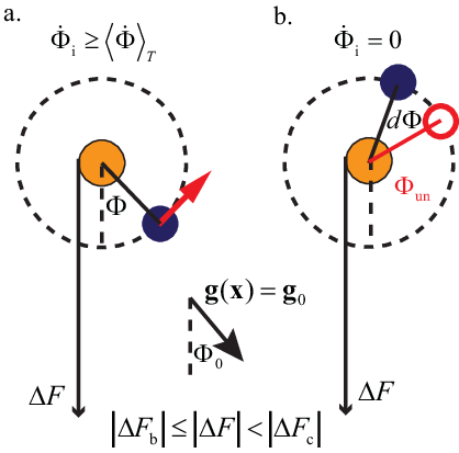
In the absence of $\alpha$ and $\Delta F$, there are two kinds of dynamic modes produced by the locking potential, i.e. uniform gravity: one is local oscillation with energy $E<g_{0}$ around the minimum of the potential; the other is rotation around the pivot with energy $E>g_{0}$. For the local oscillations, $\Delta F$ must be treated as a conservative-like forceChen et al. 2017, where the effective potential becomes $U_{\mathrm{eff}}(\Phi)=-g_{0}\cos(\Phi-\Phi_{0})-\Delta F\Phi$. By requiring $dU_{\mathrm{eff}}/d\Phi=0$ and $d^{2}U_{\mathrm{eff}}/d\Phi^{2}>0$, the unstable and stable equilibrium points are $\Phi_{\mathrm{un}}=\Phi_{0}+\pi-\sin^{-1}(\Delta F/g_{0})$ and $\Phi_{\mathrm{PL}}=\Phi_{0}+\sin^{-1}(\Delta F/g_{0})$, respectively. Thus, the stable phase-locking (PL) state $\Phi_{\mathrm{PL}}$ of Eq. (8) occurs when $|\Delta F|<g_{0}$, and $\Phi_{\mathrm{PL}}$ corresponds to the minimum of $U_{\mathrm{eff}}(\Phi)$. Obviously, there exists a upper limit value of $\Delta F$:

below which the existence of PL state can be assured.

For the rotations, i.e. asynchronized (AS) states, $\Delta F$ must be considered as a non-conservative force Chen et al. 2017, that is, a negative damping force. Thereby, one can use the theoretical approach developed in II.1 to analyze their stability. First, due to the presence of anisotropic potential, one can choose thel energy $E=\dot{\Phi}^{2}/2-g_{0}\cos(\Phi-\Phi_{0})$ as a canonical momentum $p$. By following the approach given in appendix A.1, one can easily obtain

Here, $T(p)=\int_{0}^{2\pi}d\Phi/\sqrt{2p+2g_{0}\cos(\Phi-\Phi_{0})}$ and $H_{O}(p)=2\pi\int^{p}dp^{\prime}[T(p^{\prime})]^{-1}$. Compared to Eq. (52), the positive and damping functions are $S(p)=(1/2\pi)\int_{0}^{2\pi}d\Phi\sqrt{2p+2g_{0}\cos(\Phi-\Phi_{0})}$ and $a(p,\Delta F)=(\mp)[2\pi/T(p)]\Delta F$, respectively. Accordingly, the Hamiltonian in the new frame is: $H_{N}(p)=H_{O}(p)-\int^{p}dp^{\prime}v_{p}(p^{\prime})$, where $v(p)=a(p,\Delta F)/[\alpha S(p)]$. By requiring $\partial H_{N}/\partial p=0$ and $\partial^{2}H_{N}/\partial p^{2}>0$, one can easily obtain the criteria for stable AS states labeled by $p_{0}$:

Since $\alpha S(p_{0})>0$, a minus sign must be applied to the left-hand side of the first equation for negative $\Delta F$. In addition, the second equation implies that equilibrium AS states ($p_{0}>g_{0}$) must be stable. For $p_{0}$ close to the energy minimum of an AS state, i.e. $E=g_{0}$, one can easily estimate the threshold of $\Delta F$ needed to drive the AS state:

where $S^{\prime}=\int_{0}^{2\pi}d\Phi\sqrt{1+\cos(\Phi-\Phi_{0})}\approx 5.6569$.

Note that Eq. (11) is valid for $|\Delta E|=|\int_{0}^{2\pi}d\Phi\Delta F_{\mathrm{b}}|=2\pi|\Delta F_{\mathrm{b}}|<g_{0}$ (see appendix A.1), implying that the order of $|\Delta F_{\mathrm{b}}|$ should be significantly smaller than that of $|\Delta F_{\mathrm{c}}|$. More importantly, this means there must exist a coexistent state (PL/AS) appearing within $|\Delta F_{\mathrm{b}}|<|\Delta F|<|\Delta F_{\mathrm{c}}|$. However, outside $|\Delta F_{\mathrm{b}}|<|\Delta F|<|\Delta F_{\mathrm{c}}|$, the existing stable states are only PL and AS, respectively. Moreover, Eq. (11) shows that the existent criterion for PL/AS states is dependent on the damping constant, i.e. there exists an upper limit of $\alpha$ that ensures $|\Delta F_{\mathrm{b}}|=|\Delta F_{\mathrm{c}}|$, i.e.

below which the existence of the PL/AS state can be assured.

We would like to emphasize here that due to the existence of PL/AS state, the phase-locking dynamics of a pendulum is very different from that of Adler’s equationAdler 1973. The PL/AS state also implies that even if $|\Delta F|<|\Delta F_{\mathrm{c}}|$ is satisfied, there still exist some initial states that eventually evolve into AS statesBonin et al. 2009; Tabor et al. 2010; Li et al. 2011; D’Aquino et al. 2017. This can be explained physically as follows. For a large enough frequency mismatch $|\Delta\omega|=|(F_{\textrm{dc}}/\alpha)-\omega_{e}|$, i.e. $|\Delta F_{\mathrm{b}}|<|\Delta F|<|\Delta F_{\mathrm{c}}|$, there must exist some initial states where particle gains sufficient kinetic energy from $\Delta F$ to permanently escape from the trap of the locking potential. As indicated in Fig. 3, we take two initial states apparently evolving into AS states as examples. One has a higher initial velocity than the terminal one $|\langle\dot{\Phi}\rangle_{T}|$ and is parallel to $\Delta F$; the other is initially static at the point approaching $\Phi_{\mathrm{un}}$ from its right (left) side for positive (negative) $\Delta F$. Here, $\Phi_{\mathrm{un}}$ corresponds to the maximum of the potential $U_{\mathrm{eff}}(\Phi)$. In other words, due to the assistance of sufficient kinetic energy with $\alpha<\alpha_{\mathrm{c}}$ at these states, $\Delta F_{\mathrm{b}}$ can be further lowered compared to $\Delta F_{\mathrm{c}}$. Finally, we would like to point out that due to the relationship between the non-linear frequency shift and kinetic-like energy, for any non-linear auto-oscillators, e.g. STNOs, the presence of the PL/AS state should be their common characteristic.

As shown in Fig. 4(a), one can analytically obtain the phase diagram of stable dynamic states as a function of $g_{0}$ and $\Delta F$ from Eqs. (9), (11), and (12). Moreover, when $\Delta F$ is shifted through the PL/AS state back and forth along the direction of a constant $g_{0}$ at a very slow pace, a hysteretic frequency mismatch response $\langle\dot{\Phi}\rangle_{T}$ can be observed, as shown by the gray areas of Fig. 4(b). Here, the black arrows indicate the process of hysteretic loops. When $\Delta F$ increases from PL state, i.e. $|\Delta F|<|\Delta F_{\mathrm{b}}|$ the particle will stay in PL state until $\Delta F=\pm\Delta F_{\mathrm{c}}$. Once $|\Delta F|>|\Delta F_{\mathrm{c}}|$, an abrupt jump from non-zero $\langle\dot{\Phi}\rangle_{T}$ occurs, and the dependence of $\langle\dot{\Phi}\rangle_{T}$ on $\Delta F$ can be linearly approximated by $\langle\dot{\Phi}\rangle_{T}=\Delta F/\alpha$. However, when $\Delta F$ reduces from $|\Delta F|>|\Delta F_{\mathrm{c}}|$, the particle will stay in the AS state until $|\Delta F|=|\Delta F_{\mathrm{b}}|$, and a non-linear dependence of $\langle\dot{\Phi}\rangle_{T}$ on $\Delta F$ appears, which is due to the locking potential. By solving Eq. () and using $T(p)=\int_{0}^{2\pi}d\Phi/\sqrt{2p+2g_{0}\cos(\Phi-\Phi_{0})}$, one can analytically obtain $\langle\dot{\Phi}\rangle_{T}$ as a function of $\Delta F$, as indicated by the black solid curve in Fig. 4(b). Notably, for the trajectories with an energy close to $g_{0}$, the particle will spend much more time traversing the maximum point of the potential than its minimum point, resulting in a much lower $\langle\dot{\Phi}\rangle_{T}$ relative to $\langle\dot{\Phi}\rangle_{T}=\Delta F/\alpha$.

Similarly, when one changes the amplitude of $g_{0}$ along the direction of a constant $\Delta F$ at a very slow pace, a hysteretic response $\langle\dot{\Phi}\rangle_{T}$ can be also observed, as shown in Fig. 4(c). Also, at the two ends of the hysteretic loop marked by the gray area, there exist two critical values of $g_{0}$. One indicates the bifurcation occurring at the border between AS and PL/AS states ($g_{0}=g_{0\mathrm{c}}$); the other indicates the one occurring at the border between PL/AS and AS states ($g_{0}=g_{0\mathrm{b}}$). In these, $g_{0\mathrm{c}}$ is smaller than $g_{0\mathrm{b}}$, meaning that for the locking potential with a higher energy barrier the more economic way to stimulate the AS state is relying on the assistance of kinetic energy rather than lowering the barrier hight. To summarise, the hysteretic phase-locking criterion confirms that the PL/AS state appears between the PL and AS states.

In addition to the initial state sensitivity of PL states, the pendulum-like equation also predicts the transient regime of PL states, different from that of Adler’s equation. By linearizing Eq. (8) about the stable phase-locked angle $\Phi_{\mathrm{PL}}$, i.e. $\delta\Phi\equiv\Phi-\Phi_{\mathrm{PL}}$, one can easily obtain

Here, $\omega_{0}=\sqrt{g_{0}}[1-(\Delta F/g_{0})^{2}]^{1/4}$. In the under damped case, i.e. $\omega_{0}>\alpha/2$, we obtain an oscillatory decaying solution $\delta\Phi(t)=C_{0}e^{-\alpha t/2}\cos(\omega^{\prime}t+C_{1})$, with $\omega^{\prime}=\sqrt{4\omega_{0}^{2}-\alpha^{2}}/2$. This means that the transient time of PL states is decided only by $\alpha$ rather than $g_{0}$. In the critical damped case, i.e. $\omega_{0}=\alpha/2$, the solution is $\delta\Phi(t)=(C_{0}+C_{1}t)e^{-\alpha t/2}$, where the oscillatory regime starts to disappear. In the over damped case, i.e. $\omega_{0}<\alpha/2$, the solution becomes $\delta\Phi(t)=(C_{0}e^{-i\omega^{\prime}t}+C_{1}e^{i\omega^{\prime}t})e^{-\alpha t/2}$, where the decaying transient time is dependent on $\alpha$, $g_{0}$, as well as the initial states. Notably, in this case, the initial state with more potential energy or less kinetic energy, i.e. $|C_{1}|>|C_{0}|$, will have a longer transient time scale.

Moreover, due to the periodicity of the anisotropic force in $\phi$, Eq. (7) can be generalized to the more complex case by the Fourier expansion

Here, we would like to point out that the expansion coefficients $g_{n0}$ contains not only the information about the form of the anisotropic force, but also about the geometry of the conserved trajectory. As an example, if the conservative trajectory has no axial symmetry, the projection of the force with even the simplest from, e.g. a uniform gravity, on the trajectory will also take a complicated form.

In the following, we extend the case of an individual phase-locked pendulum to that of an asymmetric pair of mutually phase-locking pendulums, which can be used to analyze the mutual phase-locking of STNO pairs. First of all, the governing equations for pendulum pairs take the following form:

Here, $\alpha_{1}\neq\alpha_{2}$ and $F_{1}\neq F_{2}$. Also, the form of the coupling force means that the two pendulums become each other’s locking potential sources, emitting effective circularly polarized oscillating uniform gravitational forces on the otherl pendulum, respectively. Moreover, using a new set of variables $\phi_{+}\equiv\phi_{1}+\phi_{2}$ and $\phi_{-}\equiv\phi_{1}-\phi_{2}$, Eq. (15) becomes

where $\alpha_{\pm}\equiv\alpha_{1}\pm\alpha_{2}$ and $F_{\pm}\equiv F_{1}\pm F_{2}$. According to Eq. (16), we know that the rotation excitation and phase-locking of the pendulum pairs are governed by $\phi_{+}$ and $\phi_{-}$ equations, respectively. Accordingly, by comparison with the free-running pendulum equation one can obtain the stable $\dot{\phi}_{+}$ as follows:

By substituting Eq. (17) into the $\phi_{-}$ equation defined by Eq. (16), one gets the $\phi_{-}$ equation decoupled with $\phi_{+}$:

Here, $\alpha^{\prime}_{+}=[\alpha_{+}-(\alpha_{-}^{2}/\alpha_{+})]/2$ and $F^{\prime}_{-}=F_{-}-\left(\alpha_{-}/\alpha_{+}\right)F_{+}$. Comparing Eqs. (18) and (8), one can easily conclude here that the hysteretic frequency response still exists in mutually phase-locked pendulum pairs. The criteria for PL/AS continue to be $|F^{\prime}_{-\mathrm{b}}|<|F^{\prime}_{-}|<|F^{\prime}_{-\mathrm{c}}|$ and $\alpha^{\prime}_{+}<\alpha^{\prime}_{+\mathrm{c}}$, where we only need to replace $\alpha$ and $\Delta F$ in Eqs. (9) and (11) by $\alpha^{\prime}_{+}$ and $F^{\prime}_{-}$, respectively.

As depicted in Fig. 5, we consider two types of electrically connected nano-pillar-based PERP-STNO pairs with an edge-to-edge separation $d_{\mathrm{ee}}$. One type is connected in parallel (Fig. 5(a)), and the other type is connected in series (Fig. 5(b)). Each pillar is composed of a spin polarizer layer (P) with a perpendicular-to-plane magnetization, a free layer (F) with an in-plane magnetization, and a synthetic antiferromagnetic (SAF) trilayer as an analyzer on top of the free layer. The thickness of the analyzing layer is designed to be one-tenth of the spin diffusion lengthHoussameddine et al. 2007, so the reflecting STT from the analyzer is relatively much smaller than that of the P layer to be neglected. Here we would like to first stress that in the parallel case the same injected current direction implies the pair of free layer magnetic moments precess with the same directionLee et al. 2005; Houssameddine et al. 2007; Chang et al. 2011; Chen et al. 2017. In contrast, in the serial case the two moments will precess in opposite directions due to the opposite injected currents.

Here we assume thatl the magnetization dynamics of the free layers are governed by the macrospin model, i.e. the Landau-Lifshitz-Gilbert-Slonczewski (LLGS) equation containing the STT effect, as detailed in Refs. Chen et al. 2016; Chen et al. 2019. Compared to Eq. (2), the vectors $\mathbf{x}$ and $\mathbf{n}$ have been both replaced by the magnetization unit vector $\mathbf{m}$ in the LLGS equation. In this model, the scaled total energy density $E$ reads as

where the cylindrical coordinate $(m_{iz},\phi_{i})$ has been used to express the energy. The terms on the right-hand side are the demagnetization and interaction energies, respectively. For $U_{I}$, we here take the magnetic dipolar interaction as an exampleChen et al. 2016; Chen et al. 2018:

where $A_{\mathrm{disc}}(d_{\mathrm{ee}})$ indicates that the dipolar coupling strength is calculated from the quasi-uniformly magnetized circular disc modelChen et al. 2016. Note that the spin polarization vector $\mathbf{z}$ coincides with the symmetric axis $\mathbf{p}$ of the demagnetization energy, so the STT here can be directly treated as a negative damping term and the Slonczewski’s asymmetirc factor in the STT can be absorbed into the negative damping factor, as indicated in Eq. (2).

In our study, the lateral dimension of FL is supposed to be $60\times 60$ $\textrm{nm}^{2}$ and the thickness $d=3$ nm. The standard material parameters of Permalloy $(\textrm{Ni}_{80}\textrm{Fe}_{20})$ are used for the FL: saturation magnetization $M_{s}=866$ $\textrm{emu}/\textrm{cm}^{3}$, and dimensionless quantities of spin-polarization efficiency $P=0.38$, and $\Lambda=1.8$Xiao et al. 2004.

Based on the axial symmetry of an individual PERP-STNO, including the demagnetization energy as well as the spin polarization vector, the canonical momentum $p_{i}\equiv-m_{iz}$. The stable OP precessional states given by $(\partial H_{Ni,0}/\partial p_{i})_{p_{i0}}=0$ and $(\partial^{2}H_{Ni,0}/\partial p_{i}^{2})_{p_{i0}}>0$ (see Appendix A.1) are

As illustrated in the dynamical state phase diagram (see Ref. Chen et al. 2019), the regions that allow field and current for $p_{i0}$ are $h_{zi}=0$ and $I_{\mathrm{u}i}<I_{i}<I_{\mathrm{c}i}$, respectively. Here $I_{\mathrm{u}i}$ and $I_{\mathrm{c}i}$ are the critical currents

and

respectively. The stability $H_{Ni,0}^{(2)}(p_{i0})$, positive damping function $S_{i}(p_{i0})$, negative damping function $a_{i}(p_{i0},\mu_{i})$, nonlinear frequency shift coefficient $H^{(2)}_{Oi}(p_{i0})$, as well as the dipolar interaction energy $U_{I}$ at $p_{i0}$ appearing in Eq. (6) are

and

respectively. Here, $\mu_{i}$ indicates the spin-polarization efficiencies $(P_{i},\Lambda_{i})$. Notably, in terms of Eq. (), the stability of OP states is mainly provided by the demagnetization energy with a blue frequency shift ($H^{(2)}_{Oi}(p_{i0})>0$), and the STT is mainly responsible for shifting the position of $p_{i0}$, which is very different from PMA-STNOs with a red frequency shift Taniguchi et al. 2013. Thus, PERP-STNO can be driven solely by current without the assistance of an external field (see also Ref.Chen et al. 2019). Compared with Eqs. (7) and (15), the magnetic dipolar coupling forces appearing in Eq. () have an anisotropy as a function of both $\phi_{-}$ and $\phi_{+}$, implying that the dipolar coupling can induce the phase-locking both in the parallel and serial connections. Note, also, that the strength of the dipolar coupling depends not only on the separation $d_{\mathrm{ee}}$ but also $p_{i0}$, and thereby, it is also dependent upon current and damping constant.

Interestingly, due to the blue frequency shift of a PERP-STNO ($H^{(2)}_{Oi}(p_{i0})>0$), its phase-locked angle will coincide with the minima of the locking potential, which is similar to the OP mode in IP-STNOs Kang et al. 2018, vortex oscillators Abreu Araujo et al. 2015, and SHE oscillators Awad et al. 2016; Awad et al. 2018. In contrast, if a certain kind of STNO has a red frequency shift ($H^{(2)}_{Oi}(p_{i0})<0$), its phase-locked angle will coincide with the maxima of the locking potential Wang et al. 2018, which is anti-parallel to that of the STNO with a blue frequency shift.

Before analyzing the phase-locking of STNO pairs, we have to further simplify Eq. (6). Firstly, since $\alpha_{i}S(p_{i0})\ll 1$, where $\alpha_{1,2}$ are both taken as $0.02$, the $2^{\mathrm{nd}}$ term on the right-hand side of Eq. (6) can be reasonably neglected. Secondly, from the expression of the last term on the right-hand side of Eq. (6) for STNO-1 as an example,

one can easily deduce two points for the parallel connection. First, $\phi_{+}$ increases with time faster than that of $\phi_{-}$, so $\langle\sin\phi_{+}\rangle_{T}\approx 0$ in the time order of $\phi_{-}$. Second, for the phase-locking state due to $\dot{\phi}_{1}\approx\dot{\phi}_{2}$, the term associated with $\sin\phi_{-}$ is also reasonably neglected. As for the serial connection, the situation is also similar. Thus, for the stable phase-locking of STNO pairs, the last term on the right-hand side of Eq. (6) can be reasonably neglected. Interestingly, this also reflects that the way that the coupling mechanism affects the STNO frequency mainly relies on shifting the canonical momentum $p_{i}$, rather than the phase angle $\phi_{i}$ directly (see also Appendix A.2)Li et al. 2010.

Subsequently, Eq. (6) for the pair of STNOs can be turned into

References

- Slonczewski (1996) J. C. Slonczewski, J. Magn. Magn. Mater. 159, L1 (1996).
- Berger (1996) L. Berger, Phys. Rev. B 54, 9353 (1996).
- Slonczewski (2002) J. Slonczewski, J. Magn. Magn. Mater. 247, 324 (2002).
- Xiao et al. (2004) J. Xiao, A. Zangwill, and M. D. Stiles, Phys. Rev. B 70, 172405 (2004).
- Hirsch (1999) J. E. Hirsch, Phys. Rev. Lett. 83, 1834 (1999).
- Kiselev et al. (2003) S. I. Kiselev et al., Nature 425, 380 (2003).
- Houssameddine et al. (2007) D. Houssameddine et al., Nat. Mater. 6, 447 (2007).
- Kubota et al. (2013) H. Kubota et al., Appl. Phys Express 6, 103003 (2013).
- Kaka et al. (2005) S. Kaka et al., Nature 437, 389 (2005).
- Pribiag et al. (2007) V. S. Pribiag et al., Nat. Phys. 3, 498 (2007).
- Khvalkovskiy et al. (2009) A. Khvalkovskiy, J. Grollier, A. Dussaux, K. Zvezdin, and V. Cros, Phys. Rev. B 80, 140401(R) (2009).
- Hoefer et al. (2010) M. A. Hoefer, T. J. Silva, and M. W. Keller, Phys. Rev. B 82, 054432 (2010).
- Xiao et al. (2017) D. Xiao et al., Phys. Rev. B 95, 024106 (2017).
- Garcia-Sanchez et al. (2016) F. Garcia-Sanchez et al., New J. Phys. 18, 075011 (2016).
- Cheng et al. (2016) R. Cheng, D. Xiao, and A. Brataas, Phys. Rev. Lett. 116, 207603 (2016).
- Khymyn et al. (2017) R. Khymyn et al., Sci. Rep. 7, 43705 (2017).
- Shen et al. (2019) L. Shen et al., Appl. Phys. Lett. 114, 042402 (2019).
- Consolo et al. (2010) G. Consolo et al., IEEE Trans. Magn. 46, 3629 (2010).
- Choi et al. (2014) H. S. Choi et al., Sci. Rep. 4, 5486 (2014).
- Romera et al. (2018) M. Romera et al., Nature 563, 230 (2018).
- Mancoff et al. (2005) F. B. Mancoff et al., Nature 437, 393 (2005).
- Grollier et al. (2006) J. Grollier, V. Cros, and A. Fert, Phys. Rev. B 73, 060409(R) (2006).
- Taniguchi et al. (2018) T. Taniguchi, S. Tsunegi, and H. Kubota, Appl. Phys Express 11, 013005 (2018).
- CHEN et al. (2011) H. CHEN, J. CHANG, and C. CHANG, SPIN 01, 1 (2011).
- Chen et al. (2012) H.-H. Chen et al., in Proc. IEEE (INTERMAG 2012), CD-01 (Taipei, Taiwan, 2012) p. 72.
- Belanovsky et al. (2012) A. D. Belanovsky, N. Locatelli, P. N. Skirdkov, F. AbreuAraujo, J. Grollier, K. A. Zvezdin, V. Cros, and A. K. Zvezdin, Phys. Rev. B 85, 100409(R) (2012).
- Abreu Araujo et al. (2015) F. Abreu Araujo et al., Phys. Rev. B 92, 045419 (2015).
- Chen et al. (2016) H. Chen, C. Lee, Z. Zhang, Y. Liu, J. Wu, L. Horng, and C. Chang, Phys. Rev. B 93, 224410 (2016).
- Kang et al. (2018) D. H. Kang et al., IEEE Trans. Nanotechnol. 17, 122 (2018).
- Chen et al. (2018) H.-H. Chen et al., SPIN 08, 1850013 (2018).
- Mancilla-Almonacid et al. (2019) D. Mancilla-Almonacid, A. Leon, R. Arias, S. Allende, and D. Altbir, Phys. Rev. E 99, 032210 (2019).
- Li et al. (2017) Y. Li, X. deMilly, F. AbreuAraujo, O. Klein, V. Cros, J. Grollier, and G. deLoubens, Phys. Rev. Lett. 118, 247202 (2017).
- Wang et al. (2017) C. Wang, D. Xiao, Y. Zhou, J. Åkerman, and Y. Liu, AIP Adv. 7, 056019 (2017).
- Wang et al. (2018) C. Wang, D. Xiao, and Y. Liu, AIP Adv. 8, 056021 (2018).
- Awad et al. (2016) A. A. Awad et al., Nat. Phys. 13, 292 (2016).
- Awad et al. (2018) A. Awad, M. Zahedinejad, P. Dürrenfeld, A. Houshang, M. Dvornik, E. Iacocca, R. Dumas, and J. Åkerman, in SPIE Nanoscience + Engineering, Vol. 10732 (SPIE, 2018).
- Chen et al. (2017) H.-H. Chen et al., J Appl Phys 121, 013902 (2017).
- Acebrón et al. (2005) J. A. Acebrón, L. L. Bonilla, C. J. Pérez Vicente, F. Ritort, and R. Spigler, Rev. Mod. Phys. 77, 137 (2005).
- Taniguchi et al. (2013) T. Taniguchi, H. Arai, S. Tsunegi, S. Tamaru, H. Kubota, and H. Imamura, Appl. Phys Express 6, 123003 (2013).
- Bonin et al. (2009) R. Bonin, G. Bertotti, C. Serpico, I. D. Mayergoyz, and M. D’Aquino, Eur. Phys. J. B 68, 221 (2009).
- Tabor et al. (2010) P. Tabor, V. Tiberkevich, A. Slavin, and S. Urazhdin, Phys. Rev. B 82, 020407(R) (2010).
- Zhou et al. (2010) Y. Zhou, V. Tiberkevich, G. Consolo, E. Iacocca, B. Azzerboni, A. Slavin, and J. Åkerman, Phys. Rev. B 82, 012408 (2010).
- Li et al. (2010) D. Li, Y. Zhou, C. Zhou, and B. Hu, Phys. Rev. B 82, 140407 (2010).
- Li et al. (2011) D. Li, Y. Zhou, B. Hu, and C. Zhou, Phys. Rev. B 84, 104414 (2011).
- D’Aquino et al. (2017) M. D’Aquino, S. Perna, A. Quercia, V. Scalera, and C. Serpico, IEEE Trans. Magn. PP, 1 (2017).
- Tortarolo et al. (2018) M. Tortarolo, B. Lacoste, J. Hem, C. Dieudonné, M.-C. Cyrille, J. A. Katine, D. Mauri, A. Zeltser, L. D. Buda-Prejbeanu, and U. Ebels, Sci. Rep. 8, 1728 (2018).
- Mayergoyz et al. (2009) I. D. Mayergoyz, G. Bertotti, and C. Serpico, Nonlinear magnetization dynamics in nanosystems (Elsevier, 2009).
- Thiele (1973) A. A. Thiele, Phys. Rev. Lett. 30, 230 (1973).
- Chen et al. (2019) H. Chen et al., SPIN 09, 1950008 (2019).
- Slavin and Tiberkevich (2009) A. Slavin and V. Tiberkevich, IEEE Trans. Magn. 45, 1875 (2009).
- Adler (1973) R. Adler, Proc. IEEE 61, 1380 (1973).
- Lee et al. (2005) K. J. Lee, O. Redon, and B. Dieny, Appl. Phys. Lett. 86, 022505 (2005).
- Chang et al. (2011) J. H. Chang, H. H. Chen, and C. R. Chang, Phys. Rev. B 83, 054425 (2011).
- Goldstein et al. (2014) H. Goldstein, C. P. Poole, and J. L. Safko, Classical Mechanics: Pearson New International Edition (Pearson Higher Ed, 2014).
- Taniguchi (2014) T. Taniguchi, Appl. Phys Express 7, 053004 (2014).
- Barone and Paterno (1982) A. Barone and G. Paterno, Physics and applications of the Josephson effect (Wiley, 1982).
- Ebels et al. (2008) U. Ebels, D. Houssameddine, I. Firastrau, D. Gusakova, C. Thirion, B. Dieny, and L. Buda-Prejbeanu, Phys. Rev. B 78, 024436 (2008).
- Chen et al. (2015) H.-H. Chen et al., IEEE Trans. Magn. 51, 1401104 (2015).