跳到论文正文
W Papers独立论文阅读器 arXiv:2003.10725 论文正文 计算阅读时间 · 0%
引用这篇论文根据当前论文元数据生成,正式投稿前建议核对。


License: arXiv.org perpetual non-exclusive license
arXiv:2003.10725v2 [math-ph] 06 Dec 2020

Three-dimensional Elastic Scattering Coefficients and Enhancement of the Elastic Near Cloaking

Hongyu Liu11 1 Corresponding Author. E-mail address: hongyu.liuip@gmail.com.  22 2 Department of Mathematics, City University of Hong Kong, Kowloon, Hong Kong SAR, China (hongyu.liuip@gmail.com; hongyliu@cityu.edu.hk).    Wing Yan Tsui33 3 Department of Mathematics, Hong Kong Baptist University, Kowloon, Hong Kong SAR, China (wytsui.yan@gmail.com).    Abdul Wahab44 4 School of Sciences and Humanities, Nazarbayev University, 53 Kabanbay Batyr Ave. Nur-Sultan 010000, Kazakhstan (abdul.wahab@nu.edu.kz).    Xianchao Wang55 5 Department of Mathematics, City University of Hong Kong, Kowloon, Hong Kong SAR, China, and School of Astronautics, Harbin Institute of Technology, Harbin 150001, Heilongjiang, China (xcwang90@gmail.com).
Abstract

This paper is concerned with the elastic near cloaking for the Lamé system in three-dimensions using the notion of elastic scattering coefficients (ESC). Accordingly, the ESC of arbitrary three-dimensional objects are designed and some of their properties are discussed using elements of the elastic layer potential theory. Then, near-cloaking structures, coined as ESC-vanishing-structures, are constructed for the elastic cloaking at a fixed frequency or a band of frequencies. These multi-layered structures are designed so that their first few significant ESC vanish ahead of transformation-elastodynamics. The invisibility effect is achieved as the arbitrary elastic object inside the cloak has near-zero scattering cross-section for a band of frequencies. The cloaking effect for the Lamé system is significantly enhanced by the proposed near-cloaking structures.

AMS subject classifications 2000. 35L05; 35R30; 74B05; 74J20; 78A46.

Key words. Elastic scattering; Scattering coefficients; Elastic cloaking; Inverse scattering.

1 Introduction

Invisibility is always the subject that draws human curiosity. A region is said to be cloaked if its contents together with the cloak are invisible and undetectable in the background for a particular class of wave measurements. Many studies on cloaking appeared in recent past thanks to the convenience of the transformation-optics. Proposals of cloaking for conductivity equations with zero frequencies were given in 2003 by Greenleaf, Lassas, and Uhlmann (see [15, 14]). Other pioneering works on transformation-optics by Pendry, Schuring, and Smith [29] and by Leonhardt [20] in 2006 gave a design for singular transformation to make objects invisible to electromagnetic waves.

Recently, the idea of transformation-optics was also applied in elastic cloaking theory [16, 13, 8, 25, 21, 28, 12]. However, it is more difficult to achieve invisibility effect in elasticity than the Maxwell equations or the Helmholtz equation for the optical waves since the Lamé system governing elastic wave propagation lacks invariance [21]. Towards this end, the idea of transformation-elastodynamics was proposed by Hu and Liu [16] in 2015 which is similar to the transformation-optics. A diffeomorphism is designed that blows up a point to form a hole (the cloaked region) and compresses the ambient space around the point to form a shell (the cloaking layer). Using the transformation-elastodynamics, an illusion is created by the customized effects on wave propagation. As the scattering measurements between the virtual space (the homogeneous background with the point) and the physical space (composed of the cloaking layer, the cloaked region, and the interface between them) are coincident, everything can be hidden to achieve an invisibility effect. Thus, the cloaking layer and anything inside it becomes hidden from the observers outside the cloaking layer.

The blow-up-a-point scheme considers a singular transformation mapping which introduces singularities for the elastic material tensors. Such singularities make both the mathematical analysis and physical application difficult. In order to avoid the singular structures, a regularized approximate cloaking scheme is considered. The general framework for constructing elastic near-cloak using the transformation-elastodynamics is introduced by Hu and Liu in [16].

In 2013, Ammari et al. [4] showed that near-cloaking from boundary measurements for the conductivity equation can be enhanced by canceling significant generalized polarization tensors (GPTs) of the cloaking device. It is established that the GPTs-vanishing structures (multi-layered coating with vanishing GPTs) can be combined with the transformation-optics, making the inclusion nearly invisible from the far-field measurements. Ammari and his coworkers also showed that similar enhancement schemes for near-cloaking can also be applied in the Helmholtz equation and Maxwell equations. For doing so, they considered the scattering cross-sections and expressed the scattering amplitudes in terms of the so-called scattering coefficients. Their multi-layered structures were designed to cancel out the scattering coefficients up to an arbitrary order. Applying the transformation-optics to the S-vanishing structures, it is established that one can enhance the invisibility effect. The numerical experiments also confirmed their results [3]. Recently, Abbas et al. [1] discussed ESC in two-dimensions and designed ESC-vanishing structures for the enhancement of the near-elastic cloaking frameworks. The study was focused on the design of two-dimensional ESC, their properties, and their reconstruction from multi-static response measurements. They briefly discussed the use of ESC for enhancing the performance of near-cloaking devices.

In this work, our aim is to apply the idea of regularized approximate elastic cloaks in [16] to improve the near-cloaking result. We extend the method of [1, 3, 4, 5, 6] to the three-dimensional elastic scattering problem in order to achieve drastically enhanced invisibility effect from the scattering cross-section measurements at a fixed frequency via transformation-elastodynamics approach. We first design three-dimensional ESC of an arbitrary elastic inclusion and introduce new multi-layered structures around the small ball in the virtual space. After vanishing the first few terms of scattering coefficients, we apply the transformation-elastodynamics to achieve invisibility. We show that arbitrary elastic object inside the cloaked region has near-zero scattering cross-section for a band of frequencies. We also substantiate that the new near-cloaking structures can enhance the cloaking effect for the Lamé system significantly. The three-dimensional ESC are not the straightforward extension of two-dimensional ESC and the design of ESC-vanishing structures in three-dimensions is much more involved than the two-dimensional case. Moreover, this study is focused on near-cloaking.

The rest of the paper is organized as follows. In Section 2, we recall a few fundamental results from the layer potential theory for scattering in linear isotropic elastic media. In Section 3, we derive the multipole expansion of the solution to the Lamé system and introduce three-dimensional ESC of an arbitrary elastic inclusion. Some of the properties of ESC are also discussed. The multi-layered structures with vanishing ESC are designed in Section 4. Section 5 deals with nearly ESC-vanishing structures and the procedure for the enhancement of nearly elastic cloaking using transformation-elastodynamics. Finally, the contributions of the paper are summarized in Section 6.

2 Elements of Layer Potential Theory

The primary concern of this article is the enhancement of the near-elastic cloaking devices using the concept of the ESC. Accordingly, our methodology is based on the integral formulations of the scattered elastic fields. Therefore, it is important to introduce the key components of the integral formulation in linear isotropic time-harmonic elasticity and provide some background material first. For details beyond those provided in this section, the readers are suggested to consult the monographs [2, 7, 18, 19].

2.1 Preliminaries and Notation

Let D⊂ℝ3D\subset\mathbb{R}^{3} be a smooth, open, and bounded domain with a connected Lipschitz boundary ∂D\partial D. Let L2​(D)L^{2}(D) be the space of square-integrable functions defined in the usual way with norm

‖v‖L2​(D):=(∫D|v|2​𝑑𝒙)1/2.\displaystyle\|v\|_{L^{2}(D)}:=\left(\int_{D}|v|^{2}d{{\itbf x}}\right)^{1/2}.

We define the Hilbert space H1​(D)H^{1}(D) by

H1(D)={v∈L2(D)|∇v∈L2(D)},\displaystyle H^{1}(D)=\left\{v\in L^{2}(D)|\quad\nabla v\in L^{2}(D)\right\},

equipped with the norm

‖v‖H1​(D)=(∫D|v|2​𝑑x+∫D|∇v|2​𝑑𝒙)1/2.\displaystyle\|v\|_{H^{1}(D)}=\left(\int_{D}|v|^{2}dx+\int_{D}|\nabla v|^{2}d{{\itbf x}}\right)^{1/2}.

We also define the Hilbert space H2​(D)H^{2}(D) containing the functions v∈H1​(D)v\in H^{1}(D) such that ∂p​qv∈L2​(D)\partial_{pq}v\in L^{2}(D) for all p,q∈{1,2,3}p,q\in\{1,2,3\}. We denote the interpolation space [H1​(D),H2​(D)]1/2[H^{1}(D),H^{2}(D)]_{1/2} by H3/2​(D)H^{3/2}(D). Let {𝐭1,𝐭2}\{\mathbf{t}_{1},\mathbf{t}_{2}\} form an orthonormal basis for the tangent plane to ∂D\partial D at point 𝒙{{\itbf x}} and ∂/∂𝐭:=∑i=12(∂/∂𝐭i)​𝐭i\partial/\partial\mathbf{t}:=\sum_{i=1}^{2}(\partial/\partial\mathbf{t}_{i})\mathbf{t}_{i} be the tangential derivative at 𝒙∈∂D{{\itbf x}}\in\partial D. Then, we say that v∈H1​(∂D)v\in H^{1}(\partial D) if v∈L2​(∂D)v\in L^{2}(\partial D) and ∂v/∂𝐭∈L2​(∂D)\partial v/\partial\mathbf{t}\in L^{2}(\partial D). We refer the interested readers to [7] for details.

Let DD be occupied by a homogeneous isotropic linear elastic material having compression modulus λ1\lambda_{1}, shear modulus μ1\mu_{1}, and volume density ρ1∈ℝ+\rho_{1}\in\mathbb{R}_{+}. Let the background domain ℝ3∖D¯\mathbb{R}^{3}\setminus\overline{D} be occupied by a different homogeneous isotropic linear elastic material having corresponding Lamé parameters (λ0,μ0)(\lambda_{0},\mu_{0}) and volume density ρ0∈ℝ+\rho_{0}\in\mathbb{R}_{+}. It is supposed that the interior and exterior Lamé parameters satisfy the strong convexity conditions, i.e.,

(1) μ0>0,3λ0+2μ0>0,μ1>0,and3λ1+2μ1>0.\displaystyle\mu_{0}>0,\quad 3\lambda_{0}+2\mu_{0}>0,\quad\mu_{1}>0,\quad\text{and}\quad 3\lambda_{1}+2\mu_{1}>0.

Moreover, it is assumed that

(2) (μ0−μ1)​(λ0−λ1)≥0and(μ0−μ1)2+(λ0−λ1)2≠0.\displaystyle(\mu_{0}-\mu_{1})(\lambda_{0}-\lambda_{1})\geq 0\quad\text{and}\quad(\mu_{0}-\mu_{1})^{2}+(\lambda_{0}-\lambda_{1})^{2}\neq 0.

Let us define the material parameters of the background medium in the presence of DD by

(3) [λ;μ;ρ]​(𝒙)=[λ0;μ0;ρ0]​χℝ3∖D¯​(𝒙)+[λ1;μ1;ρ1]​χD​(𝒙),\displaystyle[\lambda;\mu;\rho]({{\itbf x}})=[\lambda_{0};\mu_{0};\rho_{0}]\chi_{\mathbb{R}^{3}\setminus\overline{D}}({{\itbf x}})+[\lambda_{1};\mu_{1};\rho_{1}]\chi_{D}({{\itbf x}}),

where χD\chi_{D} represents the characteristic function of the domain DD.

Let ω∈ℝ+\omega\in\mathbb{R}_{+} denote the frequency of the mechanical oscillations and let 𝒖inc{{\itbf u}}^{\rm inc} be an incident time-harmonic elastic field impinging on DD with time-variations e−i​ω​te^{-i\omega t} being suppressed, i.e.,

(4) ∇⋅(ℭ0:∇𝒖inc)+ω2​ρ0​𝒖inc=𝟎,in ​ℝ3.\nabla\cdot{(\mathfrak{C}^{0}:\nabla{{\itbf u}}^{\rm inc})}+\omega^{2}\rho_{0}{{\itbf u}}^{\rm inc}=\mathbf{0},\quad\text{in }\mathbb{R}^{3}.

Here, ℭ0=(Ci​j​k​l0)i,j,k,l=13\mathfrak{C}^{0}=(C^{0}_{ijkl})_{i,j,k,l=1}^{3} is the background elasticity tensor defined by

Ci​j​k​l0=μ0​(δi​k​δj​l+δi​l​δj​k)+λ0​δi​j​δk​l,\displaystyle C^{0}_{ijkl}=\mu_{0}(\delta_{ik}\delta_{jl}+\delta_{il}\delta_{jk})+\lambda_{0}\delta_{ij}\delta_{kl},

where δi​j\delta_{ij} is the Kronecker’s delta function and ‘::’ is the contraction operator defined by

ℭ0:𝐀:=∑k,l=13Ci​j​k​l0​ak​l,\displaystyle\mathfrak{C}^{0}:\mathbf{A}:=\sum_{k,l=1}^{3}C^{0}_{ijkl}a_{kl},

for arbitrary matrix 𝐀=(ai​j)i,j=13\mathbf{A}=(a_{ij})_{i,j=1}^{3}. For ease of notation, we define the linear isotropic elasticity operator corresponding to the Lamé parameters (λ0,μ0)(\lambda_{0},\mu_{0}) by

ℒλ0,μ0[𝒘]:=(ℭ0:∇𝒘)=μ0∇𝒘+(λ0+μ0)∇∇⋅𝒘,\displaystyle\mathcal{L}_{\lambda_{0},\mu_{0}}[{{\itbf w}}]:=(\mathfrak{C}^{0}:\nabla{{\itbf w}})=\mu_{0}\nabla{{\itbf w}}+(\lambda_{0}+\mu_{0})\nabla\nabla\cdot{{\itbf w}},

for an arbitrary smooth function 𝒘:ℝ3→ℝ3{{\itbf w}}:\mathbb{R}^{3}\to\mathbb{R}^{3}. Without loss of generality, we assume that ρ0=1\rho_{0}=1, henceforth.

Let 𝒖sc{{\itbf u}}^{\rm sc} be the scattered field generated by the interaction of the incident field 𝒖inc{{\itbf u}}^{\rm inc} with DD. We define the pressure and shear parts of 𝒖sc{{\itbf u}}^{\rm sc}, respectively, by

𝒖Psc(𝒙):=−1κP2∇∇⋅𝒖sc(𝒙)and𝒖Ssc(𝒙):=1κS2∇×∇×𝒖sc(𝒙),\displaystyle{{\itbf u}}^{\rm sc}_{P}({{\itbf x}}):=\displaystyle-\frac{1}{\kappa_{P}^{2}}\nabla\nabla\cdot{{\itbf u}}^{\rm sc}({{\itbf x}})\quad\text{and}\quad{{\itbf u}}^{\rm sc}_{S}({{\itbf x}}):=\frac{1}{\kappa_{S}^{2}}\displaystyle\nabla\times\nabla\times{{\itbf u}}^{\rm sc}({{\itbf x}}),

for all 𝒙∈ℝ3∖D¯{{\itbf x}}\in\mathbb{R}^{3}\setminus{\overline{D}}. Here, the constants κP\kappa_{P} and κS\kappa_{S} are the longitudinal and transverse wave-numbers, respectively, i.e.,

κα:=ωcα,wherecP=λ0+2​μ0,cS=μ0,andα=P,S.\displaystyle\kappa_{\alpha}:=\frac{\omega}{c_{\alpha}},\quad\text{where}\quad c_{P}=\sqrt{{\lambda_{0}+2\mu_{0}}},\quad c_{S}=\sqrt{{\mu_{0}}},\quad\text{and}\quad\alpha=P,S.

It can be easily verified that 𝒖Psc{{\itbf u}}^{\rm sc}_{P} and 𝒖Ssc{{\itbf u}}^{\rm sc}_{S} satisfy

(Δ+κP2)​𝒖Psc=𝟎and(Δ+κS2)​𝒖Ssc=𝟎,in ​ℝ3∖D¯,\displaystyle\left(\Delta+\kappa_{P}^{2}\right){{\itbf u}}^{\rm sc}_{P}=\mathbf{0}\quad\text{and}\quad\left(\Delta+\kappa_{S}^{2}\right){{\itbf u}}^{\rm sc}_{S}=\mathbf{0},\quad\text{in }\mathbb{R}^{3}\setminus\overline{D},
such that ∇⋅𝒖scS=0and∇×𝒖scP=𝟎.\displaystyle\text{ such that }\nabla\cdot{{\itbf u}}^{\rm sc}_{S}=0\quad\text{and}\quad\nabla\times{{\itbf u}}^{\rm sc}_{P}=\mathbf{0}.

The scattered field is said to satisfy the Kupradze radiation condition if

lim|𝒙|→+∞|𝒙|(∂𝒖αsc∂|𝒙|−ικα𝒖αsc)=𝟎,α=P,S,ι=−1,\displaystyle\displaystyle\lim_{|{{\itbf x}}|\to+\infty}|{{\itbf x}}|\left(\frac{\partial{{\itbf u}}^{\rm sc}_{\alpha}}{\partial|{{\itbf x}}|}-\iota\kappa_{\alpha}{{\itbf u}}^{\rm sc}_{\alpha}\right)=\mathbf{0},\quad\alpha=P,S,\quad\iota=\sqrt{-1},

uniformly in all directions 𝒙^∈𝕊2:={𝒙∈ℝ3:|𝒙|=1}{\hat{{{\itbf x}}}}\in\mathbb{S}^{2}:=\{{{\itbf x}}\in\mathbb{R}^{3}\,:\,\,|{{\itbf x}}|=1\}. Here, 𝒙^:=𝒙/|𝒙|{\hat{{{\itbf x}}}}:={{\itbf x}}/|{{\itbf x}}| for any 𝒙∈ℝ3∖{𝟎}{{\itbf x}}\in\mathbb{R}^{3}\setminus\{\mathbf{0}\} and ∂/∂|𝒙|\partial/\partial|{{\itbf x}}| denotes the derivative in the radial direction.

Let 𝒖tot:=𝒖sc+𝒖inc{{\itbf u}}^{\rm tot}:={{\itbf u}}^{\rm sc}+{{\itbf u}}^{\rm inc} be the total field generated by the interaction of the incident field 𝒖inc{{\itbf u}}^{\rm inc} with DD. Then, 𝒖tot{{\itbf u}}^{\rm tot} is the solution to the Lamé system

(5) {∇⋅(ℭ:∇𝒖tot​(𝒙))+ω2​ρ​𝒖tot​(𝒙)=0,𝒙​ in ​ℝ3,𝒖sc​(𝒙)satisfies the Kupradze radiation condition as|𝒙|→+∞.\displaystyle\begin{cases}\nabla\cdot(\mathfrak{C}:\nabla{{\itbf u}}^{\rm tot}({{\itbf x}}))+\omega^{2}\rho{{\itbf u}}^{\rm tot}({{\itbf x}})=0,&{{\itbf x}}\text{ in }\mathbb{R}^{3},\\ {{\itbf u}}^{\rm sc}({{\itbf x}})\quad\text{satisfies the Kupradze radiation condition as}&|{{\itbf x}}|\to+\infty.\end{cases}

Here, ℭ\mathfrak{C} is the elasticity tensor of the elastic formation in the presence of DD and is defined in terms of the piece-wise constant parameters (λ,μ,ρ)(\lambda,\mu,\rho). It is well known that the scattering problem (5) is well-posed in H1​(ℝ3∖∂D)3H^{1}(\mathbb{R}^{3}\setminus\partial D)^{3} (see, e.g., [18, 19]).

Henceforth, the surface traction, denoted by 𝐓⁡[𝒘]\mathbf{T}[{{\itbf w}}], associated to the Lamé parameters (λ0,μ0)(\lambda_{0},\mu_{0}) is defined by

(6) 𝐓⁡[𝒘]:=𝝂⋅(ℭ:∇𝒘)=λ0​(∇⋅𝒘)​𝝂+μ0​(∇𝒘+∇𝒖⊤)​𝝂,\mathbf{T}[{{\itbf w}}]:=\bm{\nu}\cdot(\mathfrak{C}:\nabla{{\itbf w}})=\lambda_{0}(\nabla\cdot{{\itbf w}})\bm{\nu}+\mu_{0}(\nabla{{\itbf w}}+\nabla{{\itbf u}}^{\top})\bm{\nu},

for an arbitrary vector field 𝒘:ℝ3→ℂ3{{\itbf w}}:\mathbb{R}^{3}\to\mathbb{C}^{3}. Here, ∇𝒘\nabla{{\itbf w}} denotes the Jacobian matrix of 𝒘{{\itbf w}}, 𝝂\bm{\nu} is the outward unit normal vector at the boundary ∂D\partial D, and the superposed ⊤\top indicates the matrix transpose. At the interface ∂D\partial D, the solution 𝒖tot{{\itbf u}}^{\rm tot} satisfies the transmission conditions

(7) 𝒖tot|+=𝒖tot|−and𝐓⁡[𝒖tot]|+=𝐓⁡[𝒖tot]|−,{{\itbf u}}^{\rm tot}|_{+}={{{\itbf u}}^{\rm tot}|_{-}}\quad\text{and}\quad{\mathbf{T}[{{\itbf u}}^{\rm tot}]\Big|_{+}}={\mathbf{T}[{{\itbf u}}^{\rm tot}]\Big|_{-}},

where

v|±​(𝒙)=limϵ→0+v⁡(𝒙±ϵ​𝝂),𝒙∈∂D,v\big|_{\pm}({{\itbf x}})=\lim_{\epsilon\to 0^{+}}v({{\itbf x}}\pm\epsilon\bm{\nu}),\quad{{\itbf x}}\in\partial D,

for an arbitrary function vv.

2.2 Integral Representation of Scattered Field

In this section, we summarize the layer potential technique for time-harmonic linear elasticity in order to facilitate the definition of the scattering coefficients of DD. Towards this end, we first introduce the Kupradze matrix 𝚪ω\mathbf{\Gamma}^{\omega} as the fundamental solution of the time-harmonic elasticity equation in ℝ3\mathbb{R}^{3} with parameters (λ0,μ0,ρ0)(\lambda_{0},\mu_{0},\rho_{0}), i.e., 𝚪ω\mathbf{\Gamma}^{\omega} satisfies

∇⋅(ℭ0:∇𝚪ω​(𝒙))+ω2​ρ0​𝚪ω​(𝒙)=−δ𝟎​(𝒙)​𝐈3,𝒙∈ℝ3,\displaystyle\nabla\cdot\left(\mathfrak{C}^{0}:\nabla\mathbf{\Gamma}^{\omega}({{\itbf x}})\right)+\omega^{2}\rho_{0}\mathbf{\Gamma}^{\omega}({{\itbf x}})=-\delta_{\mathbf{0}}({{\itbf x}})\mathbf{I}_{3},\qquad{{\itbf x}}\in\mathbb{R}^{3},

subject to Kupradze’s outgoing radiation conditions. Here, δ𝒚\delta_{{{\itbf y}}} is the Dirac mass at 𝒚∈ℝ3{{\itbf y}}\in\mathbb{R}^{3} and 𝐈3∈ℝ3×3\mathbf{I}_{3}\in\mathbb{R}^{3\times 3} is the identity matrix. It is well known that (see, for instance, [23])

(8) 𝚪ω(𝒙)=1μ0[(𝐈2+1κS2∇∇⊤)g(𝒙,κS)−1κS2∇∇⊤g(𝒙,κP)],𝒙∈ℝ2∖{𝟎}.\mathbf{\Gamma}^{\omega}({{\itbf x}})=\frac{1}{\mu_{0}}\left[\displaystyle\left(\mathbf{I}_{2}+\frac{1}{\kappa_{S}^{2}}\nabla\nabla^{\top}\right)g({{\itbf x}},\kappa_{S})-\frac{1}{\kappa_{S}^{2}}\nabla\nabla^{\top}g({{\itbf x}},\kappa_{P})\right],\quad{{\itbf x}}\in\mathbb{R}^{2}\setminus\{\mathbf{0}\}.

The function g⁡(⋅,κα)g(\cdot,\kappa_{\alpha}), for α=P,S\alpha=P,S, is the fundamental solution to the Helmholtz operator −(Δ+κα2)-(\Delta+\kappa_{\alpha}^{2}) in ℝ3\mathbb{R}^{3} with wave-number κα∈ℝ+\kappa_{\alpha}\in\mathbb{R}_{+} (κα=κP\kappa_{\alpha}=\kappa_{P} or κS\kappa_{S}), i.e.,

Δ​g​(𝒙,κα)+κα2​g​(𝒙,κα)=−δ𝟎​(𝒙),𝒙∈ℝ3,\Delta g({{\itbf x}},\kappa_{\alpha})+\kappa_{\alpha}^{2}g({{\itbf x}},\kappa_{\alpha})=-\delta_{\bf 0}({{\itbf x}}),\quad{{\itbf x}}\in\mathbb{R}^{3},

subject to Sommerfeld’s outgoing radiation condition

lim|𝒙|→+∞|𝒙|​[∂g⁡(𝒙,κα)∂|𝒙|−ι​κα​g​(𝒙,κα)]=0,𝒙∈ℝ3.\lim_{|{{\itbf x}}|\to+\infty}|{{\itbf x}}|\left[\frac{\partial g({{\itbf x}},\kappa_{\alpha})}{\partial|{{\itbf x}}|}-\iota\kappa_{\alpha}g({{\itbf x}},\kappa_{\alpha})\right]=0,\qquad{{\itbf x}}\in\mathbb{R}^{3}.

It is easy to see that

(9) g⁡(𝒙,κα)=14​π​|𝒙|​eι​κα​|𝒙|,∀𝒙∈ℝ3∖{𝟎}.g({{\itbf x}},\kappa_{\alpha})=\displaystyle\frac{1}{4\pi|{{\itbf x}}|}e^{\iota\kappa_{\alpha}|{{\itbf x}}|},\quad\forall{{\itbf x}}\in\mathbb{R}^{3}\setminus\{\mathbf{0}\}.

In the sequel, we denote 𝚪ω​(𝒙,𝒚):=𝚪ω​(𝒙−𝒚)\mathbf{\Gamma}^{\omega}({{\itbf x}},{{\itbf y}}):=\mathbf{\Gamma}^{\omega}({{\itbf x}}-{{\itbf y}}).

Let us now introduce the elastic single-layer potential by

𝒮Dω​[𝝋]​(𝒙):=∫∂D𝚪ω​(𝒙,𝒚)​𝝋​(𝒚)​𝑑σ​(𝒚),∀𝒙∈ℝ3∖∂D,\displaystyle\mathcal{S}_{D}^{\omega}[{\bm{\varphi}}]({{\itbf x}}):=\displaystyle\int_{\partial D}\mathbf{\Gamma}^{\omega}({{\itbf x}},{{\itbf y}}){\bm{\varphi}}({{\itbf y}})d\sigma({{\itbf y}}),\quad\forall{{\itbf x}}\in\mathbb{R}^{3}\setminus\partial D,

for all densities 𝝋∈L2​(∂D)3{\bm{\varphi}}\in L^{2}(\partial D)^{3}. Here and throughout this article, d​σd\sigma denotes the infinitesimal boundary differential element. The traces 𝒮Dω​[𝝋]|±\mathcal{S}^{\omega}_{D}[{\bm{\varphi}}]\big|_{\pm} and 𝐓⁡[𝒮Dω​[𝝋]]|±\mathbf{T}\left[\mathcal{S}_{D}^{\omega}[{\bm{\varphi}}]\right]\big|_{\pm} across the interface ∂D\partial D are well-defined and satisfy the jump conditions (see, for instance, [10])

(10) {𝒮Dω​[𝝋]|+​(𝒙)=𝒮Dω​[𝝋]|−​(𝒙),𝐓⁡[𝒮Dω​[𝝋]]|±​(𝒙)=(±12​ℐ+(𝒦Dω)∗)​[𝝋]​(𝒙),a.e.𝒙∈∂D,\displaystyle\begin{cases}\displaystyle\mathcal{S}_{D}^{\omega}[{\bm{\varphi}}]\big|_{+}({{\itbf x}})=\mathcal{S}_{D}^{\omega}[{\bm{\varphi}}]\big|_{-}({{\itbf x}}),\\ \displaystyle\mathbf{T}\left[\mathcal{S}_{D}^{\omega}[{\bm{\varphi}}]\right]\big|_{\pm}({{\itbf x}})=\left(\pm\frac{1}{2}\mathcal{I}+(\mathcal{K}_{D}^{\omega})^{*}\right)[{\bm{\varphi}}]({{\itbf x}}),\quad{\rm a.e.}\quad{{\itbf x}}\in\partial D,\end{cases}

where the boundary integral operator (𝒦Dω)∗(\mathcal{K}_{D}^{\omega})^{*} is defined by

(𝒦Dω)∗​[𝝋]​(𝒙)=p.v.∫∂D𝐓⁡[𝚪ω]​(𝒙,𝒚)​𝝋​(𝒚)​𝑑σ​(𝒚),a.e.𝒙∈∂D,(\mathcal{K}_{D}^{\omega})^{*}[{\bm{\varphi}}]({{\itbf x}})={\rm p.v.}\displaystyle\int_{\partial D}\mathbf{T}\left[\mathbf{\Gamma}^{\omega}\right]({{\itbf x}},{{\itbf y}}){\bm{\varphi}}({{\itbf y}})d\sigma({{\itbf y}}),\quad{\rm a.e.}\quad{{\itbf x}}\in\partial D,

for all 𝝋∈L2​(∂D)3{\bm{\varphi}}\in L^{2}(\partial D)^{3} and p.v. stands for the Cauchy principle value of the integral. We precise that the surface traction of matrix 𝚪ω\mathbf{\Gamma}^{\omega} is defined column-wise, i.e., for all constant vectors 𝐩∈ℝ3\mathbf{p}\in\mathbb{R}^{3},

𝐓⁡[𝚪ω]​𝐩=𝐓⁡[𝚪ω​𝐩].\mathbf{T}\left[\mathbf{\Gamma}^{\omega}\right]\mathbf{p}=\mathbf{T}\left[\mathbf{\Gamma}^{\omega}\mathbf{p}\right].

In the layer potential technique, the total displacement field 𝒖tot{{\itbf u}}^{\rm tot} in the presence of inclusion DD is first represented in terms of the single-layer potentials 𝒮Dω\mathcal{S}^{\omega}_{D} and 𝒮~Dω\widetilde{\mathcal{S}}^{\omega}_{D} of unknown densities 𝝋,𝝍∈L2​(∂D)3{\bm{\varphi}},{\bm{\psi}}\in L^{2}(\partial D)^{3} as (see [2, Theorem 1.8])

(11) 𝒖tot​(𝒙,ω)={𝒖inc​(𝒙,ω)+𝒮Dω​[𝝍]​(𝒙,ω),𝒙∈ℝ3∖D¯,𝒮~Dω​[𝝋]​(𝒙,ω),𝒙∈D.{{\itbf u}}^{\rm tot}({{\itbf x}},\omega)=\begin{cases}{{\itbf u}}^{\rm inc}({{\itbf x}},\omega)+\mathcal{S}^{\omega}_{D}[{\bm{\psi}}]({{\itbf x}},\omega),&{{\itbf x}}\in\mathbb{R}^{3}\setminus\overline{D},\\ \widetilde{\mathcal{S}}^{\omega}_{D}[{\bm{\varphi}}]({{\itbf x}},\omega),&{{\itbf x}}\in D.\end{cases}

Then, the densities 𝝋,𝝍∈L2​(∂D)3{\bm{\varphi}},{\bm{\psi}}\in L^{2}(\partial D)^{3} are uniquely sought by solving the system of integral equations

(12) (𝒮~Dω−𝒮Dω𝐓~​[𝒮~Dω]|−−𝐓⁡[𝒮Dω]|+)​(𝝋𝝍)=(𝒖inc𝐓⁡[𝒖inc])|∂D.\begin{pmatrix}\widetilde{\mathcal{S}}_{D}^{\omega}&-{\mathcal{S}}_{D}^{\omega}\\ \displaystyle\widetilde{{\mathbf{T}}}[\widetilde{\mathcal{S}}_{D}^{\omega}]\Big|_{-}&\displaystyle-\mathbf{T}[\mathcal{S}_{D}^{\omega}]\Big|_{+}\end{pmatrix}\begin{pmatrix}{\bm{\varphi}}\\ {\bm{\psi}}\end{pmatrix}=\displaystyle\begin{pmatrix}{{\itbf u}}^{\rm inc}\\ \displaystyle\mathbf{T}[{{\itbf u}}^{\rm inc}]\end{pmatrix}\Bigg|_{\partial D}.

Here, the superposed ∼\sim is used to distinguish the single-layer potential and the surface traction defined using the interior parameters (λ1,μ1,ρ1)(\lambda_{1},\mu_{1},\rho_{1}). To simplify the matters, the dependence of 𝒖inc{{\itbf u}}^{\rm inc}, 𝒖sc{{\itbf u}}^{\rm sc}, 𝒖tot{{\itbf u}}^{\rm tot}, 𝝋{\bm{\varphi}}, and 𝝍{\bm{\psi}} on frequency ω\omega is suppressed unless it is necessary.

The following result from [2, Theorem 1.7] guarantees the unique solvability of system (12) and consequently that of problems (5) and (11).

Theorem 2.1.

Let DD be a Lipschitz bounded domain in ℝ3\mathbb{R}^{3} with parameters 0<λ1,μ1,ρ1<∞0<\lambda_{1},\mu_{1},\rho_{1}<\infty satisfying condition (2) and let ω2​ρ1\omega^{2}\rho_{1} be different from Dirichlet eigenvalues of the operator −ℒλ1,μ1-\mathcal{L}_{\lambda_{1},\mu_{1}} on DD. For any function 𝐮inc∈H1​(∂D)3{{\itbf u}}^{\rm inc}\in H^{1}(\partial D)^{3}, there exists a unique solution (𝛗,𝛙)∈L2​(∂D)3×L2​(∂D)3({\bm{\varphi}},{\bm{\psi}})\in L^{2}(\partial D)^{3}\times L^{2}(\partial D)^{3} to the integral system (12). Moreover, there exists a constant C>0C>0 such that

(13) ‖𝝋‖L2​(∂D)3+‖𝝍‖L2​(∂D)3≤C⁡(‖𝒖inc‖H1​(∂D)3+‖𝐓⁡[𝒖inc]‖L2​(∂D)3).\displaystyle\|{\bm{\varphi}}\|_{L^{2}(\partial D)^{3}}+\|{\bm{\psi}}\|_{L^{2}(\partial D)^{3}}\leq C\left(\|{{\itbf u}}^{\rm inc}\|_{H^{1}(\partial D)^{3}}+\left\|\mathbf{T}[{{\itbf u}}^{\rm inc}]\right\|_{L^{2}(\partial D)^{3}}\right).

3 Three-dimensional ESC

In this section, we seek the multipolar expansions of the scattered elastic field and the Kupradze matrix in terms of the spherical elastic waves. Our main goal is to introduce the ESC of an inclusion and highlight some of their important features.

3.1 Multipolar Expansions of Elastic Fields

Let 𝒙=(x1,x2,x3){{\itbf x}}=(x_{1},x_{2},x_{3}) be a point in the Cartesian coordinate system and be equivalently defined by (rsinθ𝒙cosφ𝒙,rsinθ𝒙sinφ𝒙,rcosθ𝒙)(r\sin\theta_{{\itbf x}}\cos\varphi_{{\itbf x}},r\sin\theta_{{\itbf x}}\sin\varphi_{{\itbf x}},r\cos\theta_{{\itbf x}}) in spherical coordinate system with r:=|𝒙|r:=|{{\itbf x}}|, θ𝒙∈[0,π]\theta_{{\itbf x}}\in[0,\pi], and φ𝒙∈[0,2​π)\varphi_{{\itbf x}}\in[0,2\pi). Let {𝒆r,𝒆θ,𝒆φ}\{{{\itbf e}}_{r},{{\itbf e}}_{\theta},{{\itbf e}}_{\varphi}\} be the standard orthonormal basis for the spherical coordinate system, where

(14) 𝒆r:=𝒙r,𝒆θ:=(cos⁡θ​cos⁡φ,cos⁡θ​sin⁡φ,−sin⁡θ),𝒆φ:=(−sin⁡φ,cos⁡φ,0).\displaystyle{{\itbf e}}_{r}:=\frac{{{\itbf x}}}{r},\quad{{\itbf e}}_{\theta}:=\left(\cos\theta\cos\varphi,\cos\theta\sin\varphi,-\sin\theta\right),\quad{{\itbf e}}_{\varphi}:=\left(-\sin\varphi,\cos\varphi,0\right).

For all integers n≥0n\geq 0 and m=−n,⋯,nm=-n,\cdots,n, let Yn​mY_{nm} denote the n​mnm-th spherical harmonics defined on the unit sphere 𝕊2\mathbb{S}^{2} by

Yn​m​(𝒙^):=Yn​m​(θ𝒙,φ𝒙)=(−1)m​(n−m)!​(2​n+1)4​π​(n+m)!​Pnm​(cos⁡θ𝒙)​ei​m​φ𝒙,\displaystyle Y_{nm}({\hat{{{\itbf x}}}}):=Y_{nm}(\theta_{{\itbf x}},\varphi_{{\itbf x}})=(-1)^{m}\sqrt{\frac{(n-m)!(2n+1)}{4\pi(n+m)!}}P_{n}^{m}(\cos\theta_{{\itbf x}})e^{im\varphi_{{\itbf x}}},

where PnmP^{m}_{n} is the mm-th associated Legendre function of order nn (see, e.g., [24, 2.4.78]). The vector spherical harmonics are then defined as

{𝐀n​m​(𝒙^):=𝒆r​Yn​m​(θ𝒙,φ𝒙),n≥0,𝐁n​m​(𝒙^):=1n⁡(n+1)​∇𝕊2Yn​m​(θ𝒙,φ𝒙),n>0,𝐂n​m​(𝒙^):=𝐁n​m​(θ𝒙,φ𝒙)×𝒆r,n>0,\displaystyle\begin{cases}\displaystyle\mathbf{A}_{nm}({\hat{{{\itbf x}}}}):={{\itbf e}}_{r}Y_{nm}(\theta_{{\itbf x}},\varphi_{{\itbf x}}),&n\geq 0,\\ \displaystyle\mathbf{B}_{nm}({\hat{{{\itbf x}}}}):=\frac{1}{\sqrt{n(n+1)}}\nabla_{\mathbb{S}^{2}}Y_{nm}(\theta_{{\itbf x}},\varphi_{{\itbf x}}),&n>0,\\ \displaystyle\mathbf{C}_{nm}({\hat{{{\itbf x}}}}):=\mathbf{B}_{nm}(\theta_{{\itbf x}},\varphi_{{\itbf x}})\times{{\itbf e}}_{r},&n>0,\end{cases}

where ∇𝕊2\nabla_{\mathbb{S}^{2}} denotes the surface gradient on 𝕊2\mathbb{S}^{2}, i.e.,

∇𝕊2=𝒆θ​∂∂θ+𝒆φ​1s​i​n​θ​∂∂φ.\displaystyle\nabla_{\mathbb{S}^{2}}={{\itbf e}}_{\theta}\frac{\partial}{\partial\theta}+{{\itbf e}}_{\varphi}\frac{1}{sin\theta}\frac{\partial}{\partial\varphi}.

It is well known that the vector spherical harmonics {𝐀n​m,𝐁n​m,𝐂n​m}\{\mathbf{A}_{nm},\mathbf{B}_{nm},\mathbf{C}_{nm}\} form a complete orthonormal basis of L2​(𝕊2)3L^{2}(\mathbb{S}^{2})^{3} (see, e.g., [23, p. 1900]). In fact, we have the orthogonality conditions,

(15) ∫Ω𝐀n​m⋅𝐁k​l¯​𝑑Ω=∫Ω𝐀n​m⋅𝐂k​l¯​𝑑Ω=∫Ω𝐁n​m⋅𝐂k​l¯​𝑑Ω=0,n,k>0,\displaystyle\int_{\Omega}\mathbf{A}_{nm}\cdot\overline{\mathbf{B}_{kl}}d\Omega=\int_{\Omega}\mathbf{A}_{nm}\cdot\overline{\mathbf{C}_{kl}}d\Omega=\int_{\Omega}\mathbf{B}_{nm}\cdot\overline{\mathbf{C}_{kl}}d\Omega=0,\quad n,k>0,
(16) ∫Ω𝐀n​m⋅𝐀k​l¯​𝑑Ω=∫Ω𝐁n​m⋅𝐁k​l¯​𝑑Ω=∫Ω𝐂n​m⋅𝐂k​l¯​𝑑Ω=δn​k​δm​l,\displaystyle\int_{\Omega}\mathbf{A}_{nm}\cdot\overline{\mathbf{A}_{kl}}d\Omega=\int_{\Omega}\mathbf{B}_{nm}\cdot\overline{\mathbf{B}_{kl}}d\Omega=\int_{\Omega}\mathbf{C}_{nm}\cdot\overline{\mathbf{C}_{kl}}d\Omega=\delta_{nk}\delta_{ml},

for all n≥0n\geq 0, m=−n,⋯,nm=-n,\cdots,n, k≥0k\geq 0, and l=−k,⋯,kl=-k,\cdots,k. Here, the integration is over a spherical surface Ω\Omega of unit radius with differential element d​Ω=sin⁡d​θ​d​φd\Omega=\sin d\theta d\varphi and angles (θ,φ)∈[0,π]×[0,2​π)(\theta,\varphi)\in[0,\pi]\times[0,2\pi).

Let jnj_{n} and hn(1)h^{(1)}_{n} be the order nn spherical Bessel and first kind Hankel functions, respectively. For each κα∈ℝ+\kappa_{\alpha}\in\mathbb{R}_{+}, α=P,S\alpha=P,S, n≥0n\geq 0, and m=−n,⋯,nm=-n,\cdots,n, we construct the functions vn​m​(⋅,κα)v_{nm}(\cdot,\kappa_{\alpha}) and wn​m​(⋅,κα)w_{nm}(\cdot,\kappa_{\alpha}) by

{vn​m​(𝒙,κα):=hn(1)​(κα​r)​Yn​m​(θ𝒙,φ𝒙),wn​m​(𝒙,κα):=jn​(κα​r)​Yn​m​(θ𝒙,φ𝒙).\displaystyle\begin{cases}v_{nm}({{\itbf x}},\kappa_{\alpha}):=h^{(1)}_{n}(\kappa_{\alpha}r)Y_{nm}(\theta_{{\itbf x}},\varphi_{{\itbf x}}),\\ w_{nm}({{\itbf x}},\kappa_{\alpha}):=j_{n}(\kappa_{\alpha}r)Y_{nm}(\theta_{{\itbf x}},\varphi_{{\itbf x}}).\end{cases}

The functions vn​m​(⋅,κα)v_{nm}(\cdot,\kappa_{\alpha}) and wn​m​(⋅,κα)w_{nm}(\cdot,\kappa_{\alpha}) are called the Debye’s potentials and are the outgoing radiating and entire solutions to the Helmholtz equation Δ​v+κα2​v=0\Delta v+\kappa_{\alpha}^{2}v=0 in ℝ3∖{𝟎}\mathbb{R}^{3}\setminus\{\mathbf{0}\} and ℝ3\mathbb{R}^{3}, respectively (see, e.g., [22, Theorem 9.14]).

Using vector spherical harmonics 𝐀n​m\mathbf{A}_{nm}, 𝐁n​m\mathbf{B}_{nm}, 𝐂n​m\mathbf{C}_{nm} and scalar Debye’s potentials vn​mv_{nm}, wn​mw_{nm}, we define the exterior and interior vector Debye’s potentials, for all κP,κS∈ℝ+\kappa_{P},\kappa_{S}\in\mathbb{R}_{+}, n∈ℕ∪{0}n\in\mathbb{N}\cup\{0\}, and m=−n,⋯,nm=-n,\cdots,n, respectively, as

(17) {𝐋n​m=1κP∇[vn​m(𝒙,κP)]=(hn(1))′(κPr)𝐀n​m+hn(1)​(κP​r)κP​rn⁡(n+1)𝐁n​m,n≥0,𝐌n​m=∇×[𝒙​vn​m​(𝒙,κS)]=hn(1)​(κS​r)​n⁡(n+1)​𝐂n​m,n>0,𝐍n​m=1κS∇×𝐌n​m=n⁡(n+1)κS​rhn(1)(κSr)𝐀n​m+n⁡(n+1)κS​rℋn(κSr)𝐁n​m,n>0,\displaystyle\begin{cases}\displaystyle{\mathbf{L}_{nm}}=\displaystyle\frac{1}{\kappa_{P}}\nabla[v_{nm}({{\itbf x}},\kappa_{P})]=(h_{n}^{(1)})^{\prime}(\kappa_{P}r)\mathbf{A}_{nm}+\frac{h_{n}^{(1)}(\kappa_{P}r)}{\kappa_{P}r}\sqrt{n(n+1)}{\mathbf{B}_{nm}},&n\geq 0,\\ \displaystyle{\mathbf{M}_{nm}}=\nabla\times[{{\itbf x}}v_{nm}({{\itbf x}},\kappa_{S})]=h_{n}^{(1)}(\kappa_{S}r)\sqrt{n(n+1)}\mathbf{C}_{nm},&n>0,\\ \displaystyle{\mathbf{N}_{nm}}=\frac{1}{\kappa_{S}}\nabla\times{\mathbf{M}_{nm}}=\frac{n(n+1)}{\kappa_{S}r}h_{n}^{(1)}(\kappa_{S}r){\mathbf{A}_{nm}}+\frac{\sqrt{n(n+1)}}{\kappa_{S}r}\mathcal{H}_{n}(\kappa_{S}r){\mathbf{B}_{nm}},&n>0,\end{cases}

and

(18) {𝐋~n​m=1κP∇[wn​m(𝒙,κP)]=(jn)′(κPr)𝐀n​m+jn​(κP​r)κP​rn⁡(n+1)𝐁n​m,n≥0,𝐌~n​m=∇×[𝒙​wn​m​(𝒙,κS)]=jn​(κS​r)​n⁡(n+1)​𝐂n​m,n>0,𝐍~n​m=1κS∇×𝐌~n​m=n⁡(n+1)κS​rjn(κSr)𝐀n​m+n⁡(n+1)κS​r𝒥n(κSr)𝐁n​m,n>0,\displaystyle\begin{cases}\displaystyle{\widetilde{\mathbf{L}}_{nm}}=\displaystyle\frac{1}{\kappa_{P}}\nabla[w_{nm}({{\itbf x}},\kappa_{P})]=(j_{n})^{\prime}(\kappa_{P}r)\mathbf{A}_{nm}+\frac{j_{n}(\kappa_{P}r)}{\kappa_{P}r}\sqrt{n(n+1)}{\mathbf{B}_{nm}},&n\geq 0,\\ \displaystyle{\widetilde{\mathbf{M}}_{nm}}=\nabla\times[{{\itbf x}}w_{nm}({{\itbf x}},\kappa_{S})]=j_{n}(\kappa_{S}r)\sqrt{n(n+1)}\mathbf{C}_{nm},&n>0,\\ \displaystyle{\widetilde{\mathbf{N}}_{nm}}=\frac{1}{\kappa_{S}}\nabla\times{\widetilde{\mathbf{M}}_{nm}}=\frac{n(n+1)}{\kappa_{S}r}j_{n}(\kappa_{S}r){\mathbf{A}_{nm}}+\frac{\sqrt{n(n+1)}}{\kappa_{S}r}\mathcal{J}_{n}(\kappa_{S}r){\mathbf{B}_{nm}},&n>0,\end{cases}

where ℋn​(t)=hn(1)​(t)+t​(hn(1))′​(t)\mathcal{H}_{n}(t)=h_{n}^{(1)}(t)+t{(h_{n}^{(1)})}^{\prime}(t) and 𝒥n​(t)=jn​(t)+t​(jn)′​(t)\mathcal{J}_{n}(t)=j_{n}(t)+t(j_{n})^{\prime}(t) (see, e.g., [23, p.1865-66]). Here and throughout in this paper, a prime over a function denotes the derivative with respect to its argument. It is easy to verify that the functions 𝐋n​m\mathbf{L}_{nm}, 𝐌n​m\mathbf{M}_{nm}, and 𝐍n​m\mathbf{N}_{nm} are the radiating solutions to the Lamé equation in ℝ3∖{𝟎}\mathbb{R}^{3}\setminus\{\mathbf{0}\} and 𝐋~n​m\widetilde{\mathbf{L}}_{nm}, 𝐌~n​m\widetilde{\mathbf{M}}_{nm}, and 𝐍~n​m\widetilde{\mathbf{N}}_{nm} are the entire solutions to the Lamé equation in ℝ3\mathbb{R}^{3}.

Let 𝐩{{\bf p}} be a fixed vector in ℝ3\mathbb{R}^{3}. Then, for all |𝒙|>|𝒚||{{\itbf x}}|>|{{\itbf y}}| (see, e.g., [9, Eqs. 6.73–6.74]),

𝚪ω​(𝒙−𝒚)​𝐩=\displaystyle\mathbf{\Gamma}^{\omega}({{\itbf x}}-{{\itbf y}}){{\bf p}}= ∑n=0∞ι​κPcP2​∑m=−nn𝐋n​m​(𝒙,κP)​𝐋~n​m​(𝒚,κP)¯⋅𝐩\displaystyle\sum_{n=0}^{\infty}\frac{\iota\kappa_{P}}{c_{P}^{2}}\sum_{m=-n}^{n}\mathbf{L}_{nm}({{\itbf x}},\kappa_{P})\overline{\widetilde{\mathbf{L}}_{nm}({{\itbf y}},\kappa_{P})}\cdot{{\bf p}}
+∑n=1∞ι​κSn⁡(n+1)​cS2∑m=−nn𝐌n​m(𝒙,κS)𝐌~n​m​(𝒚,κS)¯⋅𝐩\displaystyle+\sum_{n=1}^{\infty}\frac{\iota\kappa_{S}}{n(n+1)c_{S}^{2}}\sum_{m=-n}^{n}\mathbf{M}_{nm}({{\itbf x}},\kappa_{S})\overline{\widetilde{\mathbf{M}}_{nm}({{\itbf y}},\kappa_{S})}\cdot{{\bf p}}
(19) +∑n=1∞ι​κSn⁡(n+1)​cS2∑m=−nn𝐍n​m(𝒙,κS)𝐍~n​m​(𝒚,κS)¯⋅𝐩.\displaystyle+\sum_{n=1}^{\infty}\frac{\iota\kappa_{S}}{n(n+1)c_{S}^{2}}\sum_{m=-n}^{n}\mathbf{N}_{nm}({{\itbf x}},\kappa_{S})\overline{\widetilde{\mathbf{N}}_{nm}({{\itbf y}},\kappa_{S})}\cdot{{\bf p}}.

Similarly, the plane elastic waves can be also expressed in terms of the vector Debye’s potentials. In this article, we will consider the incident elastic waves of the form of either a plane shear wave

𝒖inc​(𝒙)=𝒖Sinc​(𝒙):=𝐪​eι​κS​𝒙⋅𝐝,\displaystyle{{\itbf u}}^{\rm inc}({{\itbf x}})={{\itbf u}}_{S}^{\rm inc}({{\itbf x}}):=\mathbf{q}e^{\iota\kappa_{S}{{\itbf x}}\cdot{{\bf d}}},

or a plane pressure wave

𝒖inc​(𝒙)=𝒖Pinc​(𝒙):=𝐝​eι​κP​𝒙⋅𝐝,\displaystyle{{\itbf u}}^{\rm inc}({{\itbf x}})={{\itbf u}}_{P}^{\rm inc}({{\itbf x}}):={{\bf d}}e^{\iota\kappa_{P}{{\itbf x}}\cdot{{\bf d}}},

where 𝐝∈𝕊2{{\bf d}}\in\mathbb{S}^{2} is the direction of incidence and 𝐪∈𝕊2\mathbf{q}\in\mathbb{S}^{2} is any vector orthogonal to 𝐝{{\bf d}}, i.e., 𝐪⋅𝐝=0\mathbf{q}\cdot{{\bf d}}=0. Using the vector version of the Jacobi-Anger expansion, the multipolar expansion of the plane shear wave is derived as (see, e.g., [9, Theorem 6.26])

(20) 𝒖Sinc(𝒙)=−∑k=1∞4​π​ιkk⁡(k+1)∑l=−kk\displaystyle{{\itbf u}}_{S}^{\rm inc}({{\itbf x}})=-\sum_{k=1}^{\infty}\frac{4\pi\iota^{k}}{\sqrt{k(k+1)}}\sum_{l=-k}^{k} ((𝐂k​l​(𝐝)¯⋅𝐩)​𝐌~k​l​(𝒙,κS)+ι⁡(𝐁k​l​(𝐝)¯⋅𝐩)​𝐍~k​l​(𝒙,κS)),\displaystyle\Bigg((\overline{\mathbf{C}_{kl}({{\bf d}})}\cdot{{\bf p}})\widetilde{\mathbf{M}}_{kl}({{\itbf x}},\kappa_{S})+\iota(\overline{\mathbf{B}_{kl}({{\bf d}})}\cdot{{\bf p}})\widetilde{\mathbf{N}}_{kl}({{\itbf x}},\kappa_{S})\Bigg),

where 𝐩=(𝐝×𝐪)×𝐝{{\bf p}}=({{\bf d}}\times\mathbf{q})\times{{\bf d}} with 𝐪∈ℝ3\mathbf{q}\in\mathbb{R}^{3} being the polarization direction. Similarly, the expansion of the plane pressure wave solution to the elastodynamics equation can be derived as (see, e.g., [17])

𝒖Pinc(𝒙)=−∑k=0∞4πιk+1∑l=−kk((𝐀k​l​(𝐝)¯⋅𝐝)𝐋k​l(𝒙,κP)).{{\itbf u}}^{\rm inc}_{P}({{\itbf x}})=-\sum^{\infty}_{k=0}4\pi\iota^{k+1}\sum_{l=-k}^{k}\left(\left(\overline{\mathbf{A}_{kl}({{\bf d}})}\cdot{{\bf d}}\right)\mathbf{L}_{kl}({{\itbf x}},\kappa_{P})\right).

3.2 Scattering Coefficients of Elastic Inclusions

For ease of presentation, we shall make use of the notation

𝐇k​lL​(𝒙):=𝐋k​l​(𝒙,κP),𝐇k​lM​(𝒙):=𝐌k​l​(𝒙,κS),𝐇k​lN​(𝒙):=𝐍k​l​(𝒙,κS),\displaystyle\mathbf{H}_{kl}^{L}({{\itbf x}}):=\mathbf{L}_{kl}({{\itbf x}},\kappa_{P}),\quad\mathbf{H}^{M}_{kl}({{\itbf x}}):=\mathbf{M}_{kl}({{\itbf x}},\kappa_{S}),\quad\mathbf{H}^{N}_{kl}({{\itbf x}}):=\mathbf{N}_{kl}({{\itbf x}},\kappa_{S}),
𝐉k​lL​(𝒙):=𝐋~k​l​(𝒙,κP),𝐉k​lM​(𝒙):=𝐌~k​l​(𝒙,κS),𝐉k​lN​(𝒙):=𝐍~k​l​(𝒙,κS).\displaystyle\mathbf{J}_{kl}^{L}({{\itbf x}}):=\widetilde{\mathbf{L}}_{kl}({{\itbf x}},\kappa_{P}),\quad\mathbf{J}^{M}_{kl}({{\itbf x}}):=\widetilde{\mathbf{M}}_{kl}({{\itbf x}},\kappa_{S}),\quad\mathbf{J}^{N}_{kl}({{\itbf x}}):=\widetilde{\mathbf{N}}_{kl}({{\itbf x}},\kappa_{S}).

Moreover, we reserve the notation ȷ,ȷ′=L,M,N\jmath,\jmath^{\prime}=L,M,N, and introduce nȷn_{\jmath} and kȷk_{\jmath} such that nȷ,kȷ=0n_{\jmath},k_{\jmath}=0 if ȷ=L\jmath=L and nȷ,kȷ=1n_{\jmath},k_{\jmath}=1 otherwise.

The multipolar expansion (3.1) of the Kupradze matrix 𝚪ω\mathbf{\Gamma}^{\omega} renders the series representation of the single-layer potential in terms of 𝐉n​mȷ\mathbf{J}^{\jmath}_{nm} and 𝐇n​mȷ\mathbf{H}^{\jmath}_{nm}, and subsequently, leads to the multipolar expansion of the scattered field 𝒖sc{{\itbf u}}^{\rm sc} therefrom thanks to the integral representation (11). Specifically, for 𝒙∈ℝ3∖D¯{{\itbf x}}\in\mathbb{R}^{3}\setminus\overline{D} sufficiently far from the boundary ∂D\partial D,

𝒖sc​(𝒙)=\displaystyle{{\itbf u}}^{\rm sc}({{\itbf x}})= ∑n=0∞ι​κPcP2​∑m=−nnβn​mL​𝐇n​mL​(𝒙)+∑n=1∞ι​κSn⁡(n+1)​cS2​∑m=−nnβn​mM​𝐇n​mM​(𝒙)\displaystyle\sum_{n=0}^{\infty}\frac{\iota\kappa_{P}}{c_{P}^{2}}\sum_{m=-n}^{n}\beta^{L}_{nm}\mathbf{H}^{L}_{nm}({{\itbf x}})+\sum_{n=1}^{\infty}\frac{\iota\kappa_{S}}{n(n+1)c_{S}^{2}}\sum_{m=-n}^{n}\beta^{M}_{nm}\mathbf{H}^{M}_{nm}({{\itbf x}})
+∑n=1∞ι​κSn⁡(n+1)​cS2∑m=−nnβn​mN𝐇n​mN(𝒙),\displaystyle+\sum_{n=1}^{\infty}\frac{\iota\kappa_{S}}{n(n+1)c_{S}^{2}}\sum_{m=-n}^{n}\beta^{N}_{nm}\mathbf{H}^{N}_{nm}({{\itbf x}}),

where

βn​mȷ=∫∂D𝐉n​mȷ​(𝒚)¯⋅𝝍⁡(𝒚)​𝑑σ​(𝒚).\displaystyle\beta^{\jmath}_{nm}=\int_{\partial D}\overline{\mathbf{J}^{\jmath}_{nm}({{\itbf y}})}\cdot{\bm{\psi}}({{\itbf y}})d\sigma({{\itbf y}}).

Here, (𝝋,𝝍)({\bm{\varphi}},{\bm{\psi}}) is the solution of the system of integral equations (12).

We are now fully equipped to announce the ESC of an inclusion in three-dimensions. We have the following definition.

Definition 3.1.

Let (𝛗k​lȷ,𝛙k​lȷ)({\bm{\varphi}}_{kl}^{\jmath},{\bm{\psi}}_{kl}^{\jmath}) be the solution of the integral system (12) when 𝐮inc=𝐉k​lȷ{{\itbf u}}^{\rm inc}=\mathbf{J}^{\jmath}_{kl}, for all integers k≥kȷk\geq k_{\jmath} and l=−k,⋯,kl=-k,\cdots,k. Then, the ESC, denoted by W(n,m)​(k,l)ȷ,ȷ′W_{(n,m)(k,l)}^{\jmath,\jmath^{\prime}}, for all n≥nȷn\geq n_{\jmath} and m=−n,⋯,nm=-n,\cdots,n, associated to the compression modulus λ\lambda, shear modulus μ\mu, density ρ\rho, and frequency ω\omega, is defined by

W(n,m)​(k,l)ȷ,ȷ′​[λ,μ,ρ,ω]=∫∂D𝐉n​mȷ​(𝒚)¯⋅𝝍k​lȷ′​(𝒚)​𝑑σ​(𝒚),∀ȷ,ȷ′=L,M,N.\displaystyle W_{(n,m)(k,l)}^{\jmath,\jmath^{\prime}}[\lambda,\mu,\rho,\omega]=\int_{\partial D}\overline{\mathbf{J}^{\jmath}_{nm}({{\itbf y}})}\cdot{\bm{\psi}}_{kl}^{\jmath^{\prime}}({{\itbf y}})d\sigma({{\itbf y}}),\quad\forall\,\jmath,\jmath^{\prime}=L,M,N.

The following result on the decay rate of the ESC holds.

Lemma 3.2.

For each ȷ,ȷ′=L,M,N\jmath,\jmath^{\prime}=L,M,N, there exist a constant Cȷ,ȷ′C_{\jmath,\jmath^{\prime}} depending only on the material parameters (λ,μ,ρ,ω)(\lambda,\mu,\rho,\omega) such that

|W(n,m)​(k,l)ȷ,ȷ′​[λ,μ,ρ,ω]|≤Cȷ,ȷ′n+k−2nn−1​kk−1,\displaystyle\left|W_{(n,m)(k,l)}^{\jmath,\jmath^{\prime}}[\lambda,\mu,\rho,\omega]\right|\leq\frac{C_{\jmath,\jmath^{\prime}}^{n+k-2}}{n^{n-1}k^{k-1}},

for all n≥nȷn\geq n_{\jmath}, m=−n,⋯,nm=-n,\cdots,n, k≥kȷ′k\geq k_{\jmath^{\prime}} and l=−k,⋯,kl=-k,\cdots,k.

Proof.

The proof is very similar to that of Lemma 3.1 in [6]. For the sake of completeness, we briefly sketch the proof below. First, recall that, by the Stirling’s formula, we have

k!=2​π​k​(k/e)​k​(1+O⁡(1)),as ​k→+∞.k!=\sqrt{2\pi k}(k/e)k(1+O(1)),\quad\text{as }\,k\to+\infty.

Therefore, there exists a constant C>0C>0 independent of kk such that, when k→+∞k\to+\infty and tt is fixed,

(21) jk​(t)=tk1⋅3⋯(2k+1)​(1+O⁡(1k))=O⁡(Ck​tkkk),\displaystyle j_{k}(t)=\frac{t^{k}}{1\cdot 3\cdots(2k+1)}\left(1+O\left(\frac{1}{k}\right)\right)=O\left(\frac{C^{k}t^{k}}{k^{k}}\right),

uniformly on compact subsets of ℝ\mathbb{R}. Moreover, by the recurrence formula (see, e.g., [26, Formula 10.51.2]),

(22) jk′​(t)=−jk+1​(t)+kt​jk​(t),\displaystyle j_{k}^{\prime}(t)=-j_{k+1}(t)+\frac{k}{t}j_{k}(t),

it is easy to get

(23) jk′​(t)=O⁡(Ck​tk−1kk−1),as ​k→+∞,\displaystyle j_{k}^{\prime}(t)=O\left(\frac{C^{k}t^{k-1}}{k^{k-1}}\right),\quad\text{as }\,k\to+\infty,

where the constant CC is independent of kk. Consequently, by the definition of functions 𝐉k​lȷ​(𝒙)\mathbf{J}^{\jmath}_{kl}({{\itbf x}}), Theorem 2.1, and estimates (21)-(23), we have

‖𝐉n​mȷ‖L2​(∂D)3≤(C1ȷn)n−1,\displaystyle\left\|\mathbf{J}^{\jmath}_{nm}\right\|_{L^{2}(\partial D)^{3}}\leq\left(\frac{C_{1}^{\jmath}}{n}\right)^{n-1},
‖𝝍k​lȷ′‖L2​(∂D)3≤C⁡(‖𝐉k​lȷ′‖H1​(∂D)3+‖𝐓⁡[𝐉k​lȷ′]‖L2​(∂D)3)≤(C2ȷ′k)k−1,\displaystyle\left\|{\bm{\psi}}_{kl}^{\jmath^{\prime}}\right\|_{L^{2}(\partial D)^{3}}\leq C\left(\left\|\mathbf{J}^{\jmath^{\prime}}_{kl}\right\|_{H^{1}(\partial D)^{3}}+\left\|\mathbf{T}\left[\mathbf{J}^{\jmath^{\prime}}_{kl}\right]\right\|_{L^{2}(\partial D)^{3}}\right)\leq\left(\frac{C_{2}^{\jmath^{\prime}}}{k}\right)^{k-1},

for some constants C1ȷC_{1}^{\jmath} and C2ȷ′C_{2}^{\jmath^{\prime}} dependent on material parameters and frequency ω\omega but independent of nn and kk. Finally, the proof is completed by substituting the estimates for the norms of 𝐉n​mȷ\mathbf{J}^{\jmath}_{nm} and 𝝍k​lȷ′{\bm{\psi}}_{kl}^{\jmath^{\prime}} in the definition of the ESC and choosing Cȷ,ȷ′C_{\jmath,\jmath^{\prime}} appropriately in terms of C1ȷC_{1}^{\jmath} and C2ȷ′C_{2}^{\jmath^{\prime}}. ∎

We conclude this subsection with Theorem 3.3 on the symmetry of the ESC in three-dimensions. In fact, this is the statement of the reciprocity principle for the elastic fields in terms of the ESC. The reciprocity principle in elastic media refers to the link between the far-field amplitudes of the scattered fields in two reciprocal configurations: (a) when the scattered field is radiated by a source with a specific incidence direction and is observed along another direction, (b) when the positions of the source and the observer are swapped and the orientation of all the momenta is reversed. We refer the interested readers to consult [11, 30, 31] for further discussion on the reciprocity in elastic media. The proof of Theorem 3.3 is furnished in Appendix A.

Theorem 3.3.

For all integers n≥nȷn\geq n_{\jmath}, k≥kȷ′k\geq k_{\jmath^{\prime}}, m=−n,⋯,nm=-n,\cdots,n, k=−l,⋯,lk=-l,\cdots,l, and ȷ,ȷ′=L,M,N\jmath,\jmath^{\prime}=L,M,N, we have

W(n,m),(k,l)ȷ,ȷ′​[D]=W(k,l),(n,m)ȷ′,ȷ​[D]¯.\displaystyle W^{\jmath,\jmath^{\prime}}_{(n,m),(k,l)}[D]=\overline{W^{\jmath^{\prime},\jmath}_{(k,l),(n,m)}[D]}.

3.3 Far-Field Amplitudes and Elastic Scattering Coefficients

Consider a general incident field of the form

(24) 𝒖inc=\displaystyle{{\itbf u}}^{\rm inc}= ∑k=1∞1k⁡(k+1)​∑l=−kk(bk​l​𝐉k​lM+ck​l​𝐉k​lN)+∑k=0∞∑l=−kkak​l​𝐉k​lL,\displaystyle\displaystyle\sum_{k=1}^{\infty}\frac{1}{\sqrt{k(k+1)}}\sum_{l=-k}^{k}\Bigg(b_{kl}\mathbf{J}^{M}_{kl}+c_{kl}\mathbf{J}^{N}_{kl}\Bigg)+\displaystyle\sum_{k=0}^{\infty}\sum_{l=-k}^{k}a_{kl}\mathbf{J}^{L}_{kl},

for some constants ak​la_{kl}, bk​lb_{kl}, and ck​lc_{kl}. Then, by the superposition principle, the solution 𝝍{\bm{\psi}} to the integral system (12) corresponding to 𝒖inc{{\itbf u}}^{\rm inc} in (24) is given by

(25) 𝝍=∑k=1∞1k⁡(k+1)​∑l=−kk(bk​l​𝝍k​lM+ck​l​𝝍k​lN)+∑k=0∞∑l=−kkak​l​𝝍k​lL.{\bm{\psi}}=\sum_{k=1}^{\infty}\frac{1}{\sqrt{k(k+1)}}\sum_{l=-k}^{k}\left(b_{kl}{\bm{\psi}}_{kl}^{M}+c_{kl}{\bm{\psi}}_{kl}^{N}\right)+\sum_{k=0}^{\infty}\sum_{l=-k}^{k}a_{kl}{\bm{\psi}}_{kl}^{L}.

Substituting (25) into (11) and using Definition 3.1, one can represent the scattered field 𝒖sc{{\itbf u}}^{\rm sc} as

𝒖sc​(𝒙)=\displaystyle{{\itbf u}}^{\rm sc}({{\itbf x}})= ∑n=0∞ι​κPcP2​∑m=−nnγn​mL​𝐇n​mL​(𝒙)+∑n=1∞ι​κSn⁡(n+1)​cS2​∑m=−nnγn​mM​𝐇n​mM​(𝒙)\displaystyle\sum_{n=0}^{\infty}\frac{\iota\kappa_{P}}{c_{P}^{2}}\sum_{m=-n}^{n}\gamma^{L}_{nm}\mathbf{H}^{L}_{nm}({{\itbf x}})+\sum_{n=1}^{\infty}\frac{\iota\kappa_{S}}{n(n+1)c_{S}^{2}}\sum_{m=-n}^{n}\gamma^{M}_{nm}\mathbf{H}^{M}_{nm}({{\itbf x}})
(26) +∑n=1∞ι​κSn⁡(n+1)​cS2∑m=−nnγn​mN𝐇n​mN(𝒙),as |𝒙|→+∞,\displaystyle+\sum_{n=1}^{\infty}\frac{\iota\kappa_{S}}{n(n+1)c_{S}^{2}}\sum_{m=-n}^{n}\gamma^{N}_{nm}\mathbf{H}^{N}_{nm}({{\itbf x}}),\qquad\text{as }\,|{{\itbf x}}|\to+\infty,

where, for all n≥nȷn\geq n_{\jmath}, m=−n,⋯,nm=-n,\cdots,n, and ȷ=L,M,N\jmath=L,M,N,

(27) γn​mȷ=\displaystyle\gamma^{\jmath}_{nm}= ∑k=0∞∑l=−kkak​l​W(n,m)​(k,l)ȷ,L+∑k=1∞1k⁡(k+1)​∑l=−kk(bk​l​W(n,m)​(k,l)ȷ,M+ck​l​W(n,m)​(k,l)ȷ,N).\displaystyle\sum_{k=0}^{\infty}\sum_{l=-k}^{k}a_{kl}W_{(n,m)(k,l)}^{\jmath,L}+\sum_{k=1}^{\infty}\frac{1}{\sqrt{k(k+1)}}\sum_{l=-k}^{k}\Bigg(b_{kl}W_{(n,m)(k,l)}^{\jmath,M}+c_{kl}W_{(n,m)(k,l)}^{\jmath,N}\Bigg).

On the other hand, the Kupradze radiation condition guarantees the existence of two analytic functions 𝒖P∞,𝒖S∞:𝕊2→ℂ3{{\itbf u}}^{\infty}_{P},{{\itbf u}}^{\infty}_{S}:\mathbb{S}^{2}\to\mathbb{C}^{3}, respectively called the longitudinal and transverse far-field patterns or far-field scattering amplitudes, such that

(28) 𝒖sc​(𝒙)=eι​κP​|𝒙|κP​|𝒙|​𝒖P∞​[λ,μ,ρ,ω]​(𝒙^)+eι​κS​|𝒙|κS​|𝒙|​𝒖S∞​[λ,μ,ρ,ω]​(𝒙^)+O⁡(1|𝒙|2),\displaystyle{{\itbf u}}^{\rm sc}({{\itbf x}})=\frac{e^{\iota\kappa_{P}|{{\itbf x}}|}}{\kappa_{P}|{{\itbf x}}|}{{\itbf u}}^{\infty}_{P}[\lambda,\mu,\rho,\omega](\hat{{{\itbf x}}})+\frac{e^{\iota\kappa_{S}|{{\itbf x}}|}}{\kappa_{S}|{{\itbf x}}|}{{\itbf u}}^{\infty}_{S}[\lambda,\mu,\rho,\omega](\hat{{{\itbf x}}})+O\left(\frac{1}{{|{{\itbf x}}|}^{2}}\right),

as |𝒙|→+∞|{{\itbf x}}|\to+\infty. In fact, it can be seen from (17) and (29) that the multipole fields behave as (see, e.g., [27])

𝐇Ln​m​(𝒙)∼eι​κP​|𝒙|κP​|𝒙|​(e−ι​n​π2​𝐀n​m),\displaystyle{\mathbf{H}^{L}}_{nm}({{\itbf x}})\thicksim\frac{e^{\iota\kappa_{P}|{{\itbf x}}|}}{\kappa_{P}|{{\itbf x}}|}\left(e^{-\frac{\iota n\pi}{2}}\mathbf{A}_{nm}\right),
𝐇n​mM​(𝒙)∼eι​κS​|𝒙|κS​|𝒙|​(e−ι⁡(n+1)​π2​n⁡(n+1)​𝐂n​m),\displaystyle\mathbf{H}^{M}_{nm}({{\itbf x}})\thicksim\frac{e^{\iota\kappa_{S}|{{\itbf x}}|}}{\kappa_{S}|{{\itbf x}}|}\left(e^{-\frac{\iota(n+1)\pi}{2}}\sqrt{n(n+1)}\mathbf{C}_{nm}\right),
𝐇n​mN​(𝒙)∼eι​κS​|𝒙|κS​|𝒙|​(e−ι​n​π2​n⁡(n+1)​𝐁n​m),\displaystyle\mathbf{H}^{N}_{nm}({{\itbf x}})\thicksim\frac{e^{\iota\kappa_{S}|{{\itbf x}}|}}{\kappa_{S}|{{\itbf x}}|}\left(e^{-\frac{\iota n\pi}{2}}\sqrt{n(n+1)}\mathbf{B}_{nm}\right),

since the spherical Bessel functions hn(1)h_{n}^{(1)} and (hn(1))′(h^{(1)}_{n})^{\prime} behave like

(29) (hn(1))​(t)∼1t​eι​t​e−ι⁡(n+1)​π2and(hn(1))′​(t)∼1t​eι​t​e−ι​n​π2,(h^{(1)}_{n})(t)\thicksim\frac{1}{t}e^{\iota t}e^{-\frac{\iota(n+1)\pi}{2}}\quad\text{and}\quad\left(h^{(1)}_{n}\right)^{\prime}(t)\thicksim\frac{1}{t}e^{\iota t}e^{-\frac{\iota n\pi}{2}},

as t→+∞t\to+\infty (see, e.g., [9, Eq. 2.41]). Here, f⁡(t)∼g⁡(t)f(t)\thicksim g(t) indicates that the terms of order O⁡(t−2)O(t^{-2}) are neglected, i.e, f⁡(t)=g⁡(t)+O⁡(t−2)f(t)=g(t)+O(t^{-2}). Hence, the following result holds.

Proposition 3.4.

If 𝐮inc{{\itbf u}}^{\rm inc} is of the form (24) then the corresponding scattering amplitudes of the scattered field can be represented as

(30) 𝒖P∞​[λ,μ,ρ,ω]​(𝒙^)=\displaystyle{{\itbf u}}^{\infty}_{P}[\lambda,\mu,\rho,\omega](\hat{{{\itbf x}}})= ∑n=0∞ι​κPcP2​∑m=−nnγn​mL​(e−ι​n​π2​𝐀n​m),\displaystyle\sum_{n=0}^{\infty}\frac{\iota\kappa_{P}}{c^{2}_{P}}\sum_{m=-n}^{n}\gamma^{L}_{nm}\left(e^{-\frac{\iota n\pi}{2}}\mathbf{A}_{nm}\right),
(31) 𝒖S∞​[λ,μ,ρ,ω]​(𝒙^)=\displaystyle{{\itbf u}}^{\infty}_{S}[\lambda,\mu,\rho,\omega](\hat{{{\itbf x}}})= ∑n=1∞ι​κSn⁡(n+1)​cS2​∑m=−nn[γn​mN​(e−ι⁡(n+1)​π2​𝐂n​m)+γn​mM​(e−ι​n​π2​𝐁n​m)],\displaystyle\sum_{n=1}^{\infty}\frac{\iota\kappa_{S}}{\sqrt{n(n+1)}c^{2}_{S}}\sum_{m=-n}^{n}\Bigg[\gamma^{N}_{nm}\left(e^{-\frac{\iota(n+1)\pi}{2}}\mathbf{C}_{nm}\right)+\gamma^{M}_{nm}\left(e^{-\frac{\iota n\pi}{2}}\mathbf{B}_{nm}\right)\Bigg],

where the constants γn​mȷ\gamma^{\jmath}_{nm}, for ȷ=L,M,N\jmath=L,M,N, are given in (27).

Remark 3.5.

The following remarks are in order. Since {𝐀n​m,𝐁n​m,𝐂n​m}\{\mathbf{A}_{nm},\mathbf{B}_{nm},\mathbf{C}_{nm}\} is an orthonormal set in the inner-product space, one can estimate the near-field scattering signature of the inclusion DD from its far-field scattering amplitudes by using (26) and (30)-(31). Further, if one can calculate the scattering coefficients of the inclusion DD then the scattering amplitudes 𝐮P∞{{\itbf u}}^{\infty}_{P} and 𝐮S∞{{\itbf u}}^{\infty}_{S} can also be calculated. For example, if we consider the plane shear incident wave 𝐮inc=𝐪​eι​κS​𝐱⋅𝐝{{\itbf u}}^{\rm inc}=\mathbf{q}e^{\iota\kappa_{S}{{\itbf x}}\cdot{{\bf d}}} as in (20) then

ak​l=0,bk​l=−4​π​ιk​(𝐂k​l​(𝐝)¯⋅𝐪),ck​l=−4​π​ιk+1​(𝐁k​l​(𝐝)¯⋅𝐪).a_{kl}=0,\quad b_{kl}=-4\pi\iota^{k}(\overline{\mathbf{C}_{kl}({{\bf d}})}\cdot\mathbf{q}),\quad c_{kl}=-4\pi\iota^{k+1}(\overline{\mathbf{B}_{kl}({{\bf d}})}\cdot\mathbf{q}).

Hence, the scattering amplitudes 𝐮P∞{{\itbf u}}^{\infty}_{P} and 𝐮S∞{{\itbf u}}_{S}^{\infty} defined in (30)-(31), respectively, admit the scattering coefficients

γn​mȷ=−∑k=1∞4​π​ιkk⁡(k+1)∑l=−kk((𝐂k​l​(𝐝)¯⋅𝐪)\displaystyle\gamma^{\jmath}_{nm}=-\sum_{k=1}^{\infty}\frac{4\pi\iota^{k}}{\sqrt{k(k+1)}}\sum_{l=-k}^{k}\Bigg((\overline{\mathbf{C}_{kl}({{\bf d}})}\cdot\mathbf{q}) OPENW(n,m)​(k,l)ȷ,M+ι⁡(𝐁k​l​(𝐝)¯⋅𝐪)​W(n,m)​(k,l)ȷ,N).\displaystyle W_{(n,m)(k,l)}^{\jmath,M}+\iota(\overline{\mathbf{B}_{kl}({{\bf d}})}\cdot\mathbf{q})W_{(n,m)(k,l)}^{\jmath,N}\Bigg).

4 Three-dimensional ESC-Vanishing Structures

In this section, we design concentric multi-layered spherical coatings for an elastic object so that its ESC vanish at a fixed frequency in order to construct an effective elastic cloaking device for rendering the objects inside the core invisible. These structures are coined as the ESC-vanishing structures [1, 3, 4, 5, 6].

4.1 Design of ESC-Vanishing Structure

We first choose an integer 𝔏∈ℕ\mathfrak{L}\in\mathbb{N} as a parameter for the desired number of layers and pick 𝔏+1\mathfrak{L}+1 real numbers, r1,r2,⋯,r𝔏+1∈ℝ+r_{1},r_{2},\cdots,r_{\mathfrak{L}+1}\in\mathbb{R}_{+}, such that 2=r1>r2>⋯>r𝔏+1=12=r_{1}>r_{2}>\cdots>r_{\mathfrak{L}+1}=1. Then, we construct a sequence of layers, A0,A1,⋯,A𝔏+1⊂ℝ3A_{0},A_{1},\cdots,A_{\mathfrak{L}+1}\subset\mathbb{R}^{3}, by

(32) Aℓ={ℝ3∖⋃ℓ=1𝔏+1Aℓ¯, for ​ℓ=0,{𝒙:rℓ+1≤|𝒙|<rℓ}, for ​ℓ=1,⋯,𝔏,{𝒙:|𝒙|<1}, for ​ℓ=𝔏+1,\displaystyle A_{\ell}=\begin{cases}\mathbb{R}^{3}\setminus\overline{\bigcup^{\mathfrak{L}+1}_{\ell=1}A_{\ell}},&\text{ for }\ \ell=0,\\ \{{{\itbf x}}:r_{\ell+1}\leq|{{\itbf x}}|<r_{\ell}\},&\text{ for }\ \ell=1,\cdots,\mathfrak{L},\\ \{{{\itbf x}}:|{{\itbf x}}|<1\},&\text{ for }\ \ell=\mathfrak{L}+1,\end{cases}

and denote the interfaces between the adjacent layers by Γℓ\Gamma_{\ell}. Precisely,

Γℓ:={|𝒙|=rℓ},ℓ=1,⋯,𝔏+1.\displaystyle\Gamma_{\ell}:=\{|{{\itbf x}}|=r_{\ell}\},\quad\ell=1,\cdots,\mathfrak{L}+1.

Let AℓA_{\ell}, for ℓ=1,⋯,𝔏+1\ell=1,\cdots,\mathfrak{L}+1, be loaded with an elastic material with the pair of compression and shear moduli (λℓ,μℓ)(\lambda_{\ell},\mu_{\ell}) and density ρℓ\rho_{\ell}. Accordingly, we define piece-wise constant material parameters of the entire layered elastic formation by

(33) [λ;μ;ρ]​(𝒙):=∑ℓ=0𝔏+1[λℓ;μℓ;ρℓ]​χAℓ​(𝒙),𝒙∈ℝ3.\displaystyle\left[\lambda;\mu;\rho\right]({{\itbf x}}):=\sum_{\ell=0}^{\mathfrak{L}+1}\left[\lambda_{\ell};\mu_{\ell};\rho_{\ell}\right]\chi_{A_{\ell}}({{\itbf x}}),\qquad{{\itbf x}}\in\mathbb{R}^{3}.

Further, the scattering coefficients W(n,m)​(k,l)ȷ,ȷ′W_{(n,m)(k,l)}^{\jmath,\jmath^{\prime}}, for ȷ,ȷ′=L,M,N\jmath,\jmath^{\prime}=L,M,N, are defined in this section as in Definition 3.1.

We will employ the transmission conditions on each interface Γℓ\Gamma_{\ell}, i.e., we impose

(34) 𝒖tot|+=𝒖tot|−​and​𝐓ℓ​[𝒖tot]|+=𝐓ℓ+1​[𝒖tot]|−, at ​Γℓ,ℓ=1,⋯,𝔏,{{\itbf u}}^{\rm tot}\big|_{+}={{\itbf u}}^{\rm tot}\big|_{-}\,\,\text{and}\,\,\mathbf{T}_{\ell}[{{\itbf u}}^{\rm tot}]\big|_{+}=\mathbf{T}_{\ell+1}[{{\itbf u}}^{\rm tot}]\big|_{-},\quad\text{ at }\Gamma_{\ell},\quad\ell=1,\cdots,\mathfrak{L},

where

𝐓ℓ[𝒘]:=λℓ(∇⋅𝒘)𝝂+μℓ(∇𝒖+∇𝒘⊤),ℓ=0,⋯,𝔏+1,\displaystyle\mathbf{T}_{\ell}[{{\itbf w}}]:=\lambda_{\ell}(\nabla\cdot{{\itbf w}})\bm{\nu}+\mu_{\ell}(\nabla{{\itbf u}}+\nabla{{\itbf w}}^{\top}),\quad\ell=0,\cdots,\mathfrak{L}+1,

for an arbitrary smooth function 𝒘{{\itbf w}}. It is assumed that the cloaked region, A𝔏+1A_{\mathfrak{L}+1}, is a cavity so that 𝒖tot{{\itbf u}}^{\rm tot} satisfies a traction-free boundary condition,

(35) 𝐓𝔏+1​[𝒖tot]=𝟎,on​Γ𝔏+1=∂A𝔏+1=∂𝕊2.\mathbf{T}_{\mathfrak{L}+1}[{{\itbf u}}^{\rm tot}]=\mathbf{0},\qquad\text{on}\ \Gamma_{\mathfrak{L}+1}=\partial A_{\mathfrak{L}+1}=\partial\mathbb{S}^{2}.

We have the following definition of a three-dimensional ESC-vanishing structure.

Definition 4.1.

The multi-layered medium (32) together with parameters (λ,μ,ρ)(\lambda,\mu,\rho) defined in (33) is called the ESC-vanishing structure at frequency ω\omega if W(n,m)​(k,l)ȷ,ȷ′=0W_{(n,m)(k,l)}^{\jmath,\jmath^{\prime}}=0 for all ȷ,ȷ′=L,M,N\jmath,\jmath^{\prime}=L,M,N, integers n≥nȷn\geq n_{\jmath}, k≥kȷ′k\geq k_{\jmath^{\prime}}, m=−n,⋯,nm=-n,\cdots,n, and l=−k,⋯,kl=-k,\cdots,k.

In order to design the ESC-vanishing structure, it suffices to find appropriate (λ,μ,ρ)(\lambda,\mu,\rho) such that W(n,m)​(k,l)ȷ,ȷ′=0W_{(n,m)(k,l)}^{\jmath,\jmath^{\prime}}=0. In the rest of this section, we establish constitutive relations in order to design parameters (λ,μ,ρ)(\lambda,\mu,\rho) . Towards this end, we seek the solution 𝒖n​mtot{{\itbf u}}_{nm}^{\rm tot} of Lamé system (5) of the form

𝒖n​mtot(𝒙)=𝒖n​minc(𝒙)+𝒖n​msc(𝒙),n>0,m=−n,⋯,n,\displaystyle{{\itbf u}}_{nm}^{\rm tot}({{\itbf x}})={{\itbf u}}_{nm}^{\rm inc}({{\itbf x}})+{{\itbf u}}_{nm}^{\rm sc}({{\itbf x}}),\qquad n>0,\quad m=-n,\cdots,n,

with

𝒖n​minc​(𝒙)=∑ȷ=L,M,Naℓȷ​𝐉ȷn​m​(𝒙),\displaystyle{{\itbf u}}_{nm}^{\rm inc}{({{\itbf x}})}=\sum_{\jmath=L,M,N}a^{\jmath}_{\ell}{\mathbf{J}^{\jmath}}_{nm}({{\itbf x}}), 𝒙∈Aℓ,ℓ=0,⋯,𝔏,\displaystyle{{\itbf x}}\in A_{\ell},\,\,\ell=0,\cdots,\mathfrak{L},
𝒖n​msc​(𝒙)=∑ȷ=L,M,Nbℓȷ​𝐇ȷn​m​(𝒙),\displaystyle{{\itbf u}}_{nm}^{\rm sc}({{\itbf x}})=\sum_{\jmath=L,M,N}b^{\jmath}_{\ell}{\mathbf{H}^{\jmath}}_{nm}({{\itbf x}}), 𝒙∈Aℓ,ℓ=0,⋯,𝔏,\displaystyle{{\itbf x}}\in A_{\ell},\,\ell=0,\cdots,\mathfrak{L},

where the coefficients aℓȷ,bℓȷ∈ℂa^{\jmath}_{\ell},b^{\jmath}_{\ell}\in\mathbb{C}, for ℓ=0,⋯,𝔏\ell=0,\cdots,\mathfrak{L}, are to be determined subject to

(a0L)2+(a0M)2+(a0N)2≠0andb0ȷ=0,for all ​ȷ=L,M,N.\displaystyle(a_{0}^{L})^{2}+(a_{0}^{M})^{2}+(a_{0}^{N})^{2}\neq 0\quad\text{and}\quad b_{0}^{\jmath}=0,\quad\text{for all }\,\jmath=L,M,N.

In fact, the coefficients a0ȷa_{0}^{\jmath} control the proportion of 𝐉n​mȷ\mathbf{J}^{\jmath}_{nm} in the incident field whereas b0ȷb_{0}^{\jmath} control the proportion of 𝐇ȷ\mathbf{H}^{\jmath} in the scattered field. By comparison with multipolar expansion (26)-(27), it is evident that

(36) W(n,m)​(k,l)ȷ,ȷ′=ζ0ȷ​b0ȷwhen​a0ȷ′′=δȷ′​ȷ′′,∀ȷ,ȷ′,ȷ′′=L,M,N.\displaystyle W_{(n,m)(k,l)}^{\jmath,\jmath^{\prime}}=\zeta^{\jmath}_{0}\,b^{\jmath}_{0}\quad\text{when}\,\,a_{0}^{\jmath^{\prime\prime}}=\delta_{\jmath^{\prime}\jmath^{\prime\prime}},\qquad\forall\jmath,\jmath^{\prime},\jmath^{\prime\prime}=L,M,N.

Here,

ζ0L:=−ι​cP,𝔏+12κP,𝔏+1,andζ0N=ζ0M:=−ι​n​(n+1)​cS,𝔏+12κS,𝔏+1,\displaystyle\zeta^{L}_{0}:=-\frac{\iota c_{P,\mathfrak{L}+1}^{2}}{\kappa_{P,\mathfrak{L}+1}},\quad\text{and}\quad\zeta^{N}_{0}=\zeta^{M}_{0}:=-\frac{\iota n(n+1)c_{S,\mathfrak{L}+1}^{2}}{\kappa_{S,\mathfrak{L}+1}},

with

cP,ℓ=λℓ+2​μℓρℓ,cS,ℓ=μℓρℓ,κα,ℓ=ωcα,ℓ,∀ℓ=0,⋯,𝔏+1.\displaystyle c_{P,\ell}=\sqrt{\frac{\lambda_{\ell}+2\mu_{\ell}}{\rho_{\ell}}},\quad c_{S,\ell}=\sqrt{\frac{\mu_{\ell}}{\rho_{\ell}}},\quad\kappa_{\alpha,\ell}=\frac{\omega}{c_{\alpha,\ell}},\qquad\forall\ell=0,\cdots,\mathfrak{L}+1.

4.2 Determination of Coefficients aℓȷa_{\ell}^{\jmath} and bℓȷb_{\ell}^{\jmath}

In order to determine the coefficients aℓȷa_{\ell}^{\jmath} and bℓȷb_{\ell}^{\jmath}, we require six equations for each ℓ=1,⋯,𝔏+1\ell=1,\cdots,\mathfrak{L}+1. Towards this end, we will effectively use the transmission conditions (34) and the traction-free boundary condition (35).

We first use the transmission condition in (34) for the Dirichlet data to get

∑ȷ=L,M,N[aℓ−1ȷ​[𝐉n​mȷ]ℓ−1+bℓ−1ȷ​[𝐇n​mȷ]ℓ−1]\displaystyle\sum_{\jmath=L,M,N}\Big[a^{\jmath}_{\ell-1}{[\mathbf{J}^{\jmath}_{nm}]}_{\ell-1}+b^{\jmath}_{\ell-1}{[\mathbf{H}^{\jmath}_{nm}]}_{\ell-1}\Big]
(37) =∑ȷ=L,M,N[aℓȷ[𝐉n​mȷ]ℓ+bℓȷ[𝐇n​mȷ]ℓ],on Γℓ for ℓ=1,⋯,𝔏,\displaystyle\qquad\qquad=\sum_{\jmath=L,M,N}\Big[a^{\jmath}_{\ell}[\mathbf{J}^{\jmath}_{nm}]_{\ell}+b^{\jmath}_{\ell}[\mathbf{H}^{\jmath}_{nm}]_{\ell}\Big],\quad\text{on }\,\Gamma_{\ell}\,\text{ for }\,\ell=1,\cdots,\mathfrak{L},

where the notation [𝒘]ℓ[{{\itbf w}}]_{\ell} indicates that the quantity 𝒘{{\itbf w}} is associated to the parameters (λℓ,μℓ,ρℓ)(\lambda_{\ell},\mu_{\ell},\rho_{\ell}) and to the corresponding wave-numbers κα,ℓ\kappa_{\alpha,\ell}. Substituting the expressions (17)-(18) for the vector potentials 𝐉n​mȷ\mathbf{J}^{\jmath}_{nm} and 𝐇n​mȷ\mathbf{H}^{\jmath}_{nm} into (37), we get

[En]ℓ−1​(rℓ)​𝐀n​m\displaystyle[E_{n}]_{\ell-1}(r_{\ell})\mathbf{A}_{nm} +[Fn]ℓ−1​(rℓ)​𝐁n​m+[Gn]ℓ−1​(rℓ)​𝐂n​m\displaystyle+[F_{n}]_{\ell-1}(r_{\ell}){\mathbf{B}_{nm}}+[G_{n}]_{\ell-1}(r_{\ell})\mathbf{C}_{nm}
(38) =\displaystyle= [En]ℓ​(rℓ)​𝐀n​m+[Fn]ℓ​(rℓ)​𝐁n​m+[Gn]ℓ​(rℓ)​𝐂n​m,\displaystyle[E_{n}]_{\ell}(r_{\ell})\mathbf{A}_{nm}+[F_{n}]_{\ell}(r_{\ell})\mathbf{B}_{nm}+[G_{n}]_{\ell}(r_{\ell})\mathbf{C}_{nm},

for all ℓ=1,⋯,𝔏\ell=1,\cdots,\mathfrak{L}, with

(39) [En]ℓ​(r)=\displaystyle[E_{n}]_{\ell}(r)= aℓL​(jn)′​(κP,ℓ​r)+aℓN​n⁡(n+1)κS,ℓ​r​jn​(κS,ℓ​r)+bℓL​(hn(1))′​(κP,ℓ​r)+bℓN​n⁡(n+1)κS,ℓ​r​hn(1)​(κS,ℓ​r),\displaystyle a^{L}_{\ell}(j_{n})^{\prime}(\kappa_{P,\ell}r)+a^{N}_{\ell}\frac{n(n+1)}{\kappa_{S,\ell}r}j_{n}(\kappa_{S,\ell}r)+b^{L}_{\ell}(h_{n}^{(1)})^{\prime}(\kappa_{P,\ell}r)+b^{N}_{\ell}\frac{n(n+1)}{\kappa_{S,\ell}r}h_{n}^{(1)}(\kappa_{S,\ell}r),
(40) [Fn]ℓ​(r)=\displaystyle[F_{n}]_{\ell}(r)= [aℓL​jn​(κP,ℓ​r)κP,ℓ​r+aℓN​𝒥n​(κS,ℓ​r)κS,ℓ​r+bℓL​hn(1)​(κP,ℓ​r)κP,ℓ​r+bℓN​ℋn​(κS,ℓ​r)κS,ℓ​r]​n⁡(n+1),\displaystyle\Bigg[a^{L}_{\ell}\frac{j_{n}(\kappa_{P,\ell}r)}{\kappa_{P,\ell}r}+a^{N}_{\ell}\frac{\mathcal{J}_{n}(\kappa_{S,\ell}r)}{\kappa_{S,\ell}r}+b^{L}_{\ell}\frac{h_{n}^{(1)}(\kappa_{P,\ell}r)}{\kappa_{P,\ell}r}+b^{N}_{\ell}\frac{\mathcal{H}_{n}(\kappa_{S,\ell}r)}{\kappa_{S,\ell}r}\Bigg]\sqrt{n(n+1)},
(41) [Gn]ℓ​(r)=\displaystyle[G_{n}]_{\ell}(r)= [aℓM​jn​(κS,ℓ​r)+bℓM​hn(1)​(κS,ℓ​r)]​n⁡(n+1).\displaystyle\Big[a^{M}_{\ell}j_{n}({\kappa_{S,\ell}r})+b^{M}_{\ell}h_{n}^{(1)}(\kappa_{S,\ell}r)\Big]\sqrt{n(n+1)}.

Therefore, multiplying (38) with 𝐀k​l¯\overline{\mathbf{A}_{kl}}, 𝐁k​l¯\overline{\mathbf{B}_{kl}}, and 𝐂k​l¯\overline{\mathbf{C}_{kl}}, respectively, to form a dot product and then applying orthogonality conditions (15)-(16), one gets three recursive relations,

[En]ℓ−1=[En]ℓ,[Fn]ℓ−1=[Fn]ℓ,[Gn]ℓ−1=[Gn]ℓ,on Γℓ,\displaystyle[E_{n}]_{\ell-1}=[E_{n}]_{\ell},\quad[F_{n}]_{\ell-1}={[F_{n}]}_{\ell},\quad[G_{n}]_{\ell-1}=[G_{n}]_{\ell},\quad\text{on }\,\Gamma_{\ell},

for n∈ℕn\in\mathbb{N}, m=−n,⋯,nm=-n,\cdots,n, and ℓ=1,⋯,𝔏\ell=1,\cdots,\mathfrak{L}. In the same spirit, we form another set of three equations using the transmission condition (34) for the surface traction and subsequently invoking the orthogonality conditions (15)-(16). The interested readers are referred to Appendix B for the expressions of the surface traction for different multipole elastic fields.

The aforementioned procedure renders six simultaneous equations in six unknowns that can be written in a matrix form as

(42) [[𝐏nL,N]ℓ​(rℓ)𝟎4×2𝟎2×4[𝐏nM]ℓ​(rℓ)]​[aℓLaℓNbℓLbℓNaℓMbℓM]=[[𝐏nL,N]ℓ−1​(rℓ)𝟎4×2𝟎2×4[𝐏nM]ℓ−1​(rℓ)]​[aℓ−1Laℓ−1Nbℓ−1Lbℓ−1Naℓ−1Mbℓ−1M],\begin{bmatrix}[\mathbf{P}_{n}^{L,N}]_{\ell}(r_{\ell})&\mathbf{0}_{4\times 2}\\ \\ \mathbf{0}_{2\times 4}&[\mathbf{P}_{n}^{M}]_{\ell}(r_{\ell})\end{bmatrix}\begin{bmatrix}a^{L}_{\ell}\\ a^{N}_{\ell}\\ b^{L}_{\ell}\\ b^{N}_{\ell}\\ a^{M}_{\ell}\\ b^{M}_{\ell}\end{bmatrix}=\begin{bmatrix}[\mathbf{P}_{n}^{L,N}]_{\ell-1}(r_{\ell})&\mathbf{0}_{4\times 2}\\ \\ \mathbf{0}_{2\times 4}&[\mathbf{P}_{n}^{M}]_{\ell-1}(r_{\ell})\end{bmatrix}\begin{bmatrix}a^{L}_{\ell-1}\\ a^{N}_{\ell-1}\\ b^{L}_{\ell-1}\\ b^{N}_{\ell-1}\\ a^{M}_{\ell-1}\\ b^{M}_{\ell-1}\end{bmatrix},

where [𝐏nL,N]ℓ​(rℓ):=[𝐏nL,N]ℓ​(rℓ,λ,μ,ρ,ω){[\mathbf{P}_{n}^{L,N}]}_{\ell}(r_{\ell}):={[\mathbf{P}_{n}^{L,N}]}_{\ell}(r_{\ell};\lambda,\mu,\rho,\omega) is a 4×44\times 4 sub-matrix corresponding to the fields (𝐉n​mL,𝐉n​mN,𝐇n​mL,𝐇n​mN)(\mathbf{J}^{L}_{nm},\mathbf{J}^{N}_{nm},\mathbf{H}^{L}_{nm},\mathbf{H}^{N}_{nm}), whereas [𝐏nM]ℓ​(rℓ):=[𝐏nM]ℓ​(rℓ,λ,μ,ρ,ω)[\mathbf{P}_{n}^{M}]_{\ell}(r_{\ell}):=[\mathbf{P}_{n}^{M}]_{\ell}(r_{\ell};\lambda,\mu,\rho,\omega) is a 2×22\times 2 sub-matrix corresponding to (𝐉n​mM,𝐇n​mM)(\mathbf{J}^{M}_{nm},\mathbf{H}^{M}_{nm}). The expressions of the elements of [𝐏nL,N]ℓ{[\mathbf{P}_{n}^{L,N}]}_{\ell} and [𝐏nM]ℓ{[\mathbf{P}_{n}^{M}]}_{\ell} can be found in C. It is worth mentioning that the sub-matrices [𝐏nL,N]ℓ[\mathbf{P}_{n}^{L,N}]_{\ell} and [𝐏nM]ℓ[\mathbf{P}_{n}^{M}]_{\ell} are invertible. Therefore, matrix equation (42) yields a recursive relation

(43) [aℓLaℓNbℓLbℓNaℓMbℓM]=[[𝐏nL,N]ℓ−1​[𝐏nL,N]ℓ−1𝟎4×2𝟎2×4[𝐏nM]ℓ−1​[𝐏nM]ℓ−1]​[aℓ−1Laℓ−1Nbℓ−1Lbℓ−1Naℓ−1Mbℓ−1M],\begin{bmatrix}a^{L}_{\ell}\\ a^{N}_{\ell}\\ b^{L}_{\ell}\\ b^{N}_{\ell}\\ a^{M}_{\ell}\\ b^{M}_{\ell}\end{bmatrix}=\begin{bmatrix}[\mathbf{P}_{n}^{L,N}]_{\ell}^{-1}[\mathbf{P}_{n}^{L,N}]_{\ell-1}&\mathbf{0}_{4\times 2}\\ \\ \mathbf{0}_{2\times 4}&[\mathbf{P}_{n}^{M}]_{\ell}^{-1}[\mathbf{P}_{n}^{M}]_{\ell-1}\end{bmatrix}\begin{bmatrix}a^{L}_{\ell-1}\\ a^{N}_{\ell-1}\\ b^{L}_{\ell-1}\\ b^{N}_{\ell-1}\\ a^{M}_{\ell-1}\\ b^{M}_{\ell-1}\end{bmatrix},

for all ℓ=1,⋯𝔏\ell=1,\cdots\mathfrak{L}.

In order to solve the recursive relation (43), we invoke the zero-traction condition (35) on Γ𝔏+1(i.e.,r𝔏+1=1)\Gamma_{\mathfrak{L}+1}(i.e.,r_{\mathfrak{L}+1}=1). This furnishes

(44) [000000]=[[𝐐nL,N]𝔏𝟎4×2𝟎2×4[𝐐nM]𝔏]​[a𝔏La𝔏Nb𝔏Lb𝔏Na𝔏Mb𝔏M],\begin{bmatrix}0\\ 0\\ 0\\ 0\\ 0\\ 0\end{bmatrix}=\begin{bmatrix}{[\mathbf{Q}_{n}^{L,N}]}_{\mathfrak{L}}&\mathbf{0}_{4\times 2}\\ \\ \mathbf{0}_{2\times 4}&{[\mathbf{Q}_{n}^{M}]}_{\mathfrak{L}}\end{bmatrix}\begin{bmatrix}a^{L}_{\mathfrak{L}}\\ a^{N}_{\mathfrak{L}}\\ b^{L}_{\mathfrak{L}}\\ b^{N}_{\mathfrak{L}}\\ a^{M}_{\mathfrak{L}}\\ b^{M}_{\mathfrak{L}}\end{bmatrix},

where [𝐐nL,N]𝔏[\mathbf{Q}_{n}^{L,N}]_{\mathfrak{L}} and [𝐐nM]𝔏[\mathbf{Q}_{n}^{M}]_{\mathfrak{L}} are 4×44\times 4 and 2×22\times 2 sub-matrices, respectively and the superscripts indicate their dependence on different wave-modes. The expressions of the elements of these matrices are also provided in Appendix C.

Substituting (43) into (44), one arrives at

(45) [000000]=[𝐑nL,N𝟎4×2𝟎2×4𝐑nM]​[a0La0Nb0Lb0Na0Mb0M],\begin{bmatrix}0\\ 0\\ 0\\ 0\\ 0\\ 0\end{bmatrix}=\begin{bmatrix}\mathbf{R}_{n}^{L,N}&\mathbf{0}_{4\times 2}\\ \\ \mathbf{0}_{2\times 4}&\mathbf{R}_{n}^{M}\end{bmatrix}\begin{bmatrix}a^{L}_{0}\\ a^{N}_{0}\\ b^{L}_{0}\\ b^{N}_{0}\\ a^{M}_{0}\\ b^{M}_{0}\end{bmatrix},

where

(46) {𝐑nL,N​[λ,μ,ρ,ω]:=((RnL,N)p,q)=[𝐐nL,N]𝔏​∏ℓ=1𝔏[𝐏nL,N]ℓ(−1)​[𝐏nL,N]ℓ−1,𝐑nM​[λ,μ,ρ,ω]:=((RnM)p,q)=[𝐐nM]𝔏​∏ℓ=1𝔏[𝐏nM]ℓ(−1)​[𝐏nM]ℓ−1.\displaystyle\begin{cases}\mathbf{R}_{n}^{L,N}[\lambda,\mu,\rho,\omega]:=\left({(R_{n}^{L,N})}_{p,q}\right)=\displaystyle[\mathbf{Q}_{n}^{L,N}]_{\mathfrak{L}}\prod_{\ell=1}^{{\mathfrak{L}}}[\mathbf{P}_{n}^{L,N}]_{\ell}^{(-1)}{[\mathbf{P}_{n}^{L,N}]}_{\ell-1},\\ \mathbf{R}_{n}^{M}[\lambda,\mu,\rho,\omega]:=\left({(R_{n}^{M})}_{p,q}\right)=\displaystyle[\mathbf{Q}_{n}^{M}]_{\mathfrak{L}}\prod_{\ell=1}^{\mathfrak{L}}[\mathbf{P}_{n}^{M}]_{\ell}^{(-1)}[\mathbf{P}_{n}^{M}]_{\ell-1}.\end{cases}

4.3 Constitutive Equations for Material Parameters

If we consider an incident pressure wave 𝐉n​mL\mathbf{J}^{L}_{nm} for n>0n>0 (i.e., a0L=1a_{0}^{L}=1, a0M=0a_{0}^{M}=0, and a0N=0a_{0}^{N}=0) then (45) renders

(47) {(RnL,N)1,1+b0L​(RnL,N)1,3+b0N​(RnL,N)1,4=0,(RnL,N)2,1+b0L​(RnL,N)2,3+b0N​(RnL,N)2,4=0,b0M=0.\displaystyle\begin{cases}\displaystyle(R^{L,N}_{n})_{1,1}+b^{L}_{0}(R^{L,N}_{n})_{1,3}+b^{N}_{0}(R^{L,N}_{n})_{1,4}&=0,\\ \ \displaystyle(R^{L,N}_{n})_{2,1}+b^{L}_{0}(R^{L,N}_{n})_{2,3}+b^{N}_{0}(R^{L,N}_{n})_{2,4}&=0,\\ \displaystyle b^{M}_{0}&=0.\end{cases}

Solving system of equations (47), we get

(48) {b0L​L:=b0L=(RnL,N)1,1​(RnL,N)2,4−(RnL,N)1,4​(RnL,N)2,1(RnL,N)1,4​(RnL,N)2,3−(RnL,N)1,3​(RnL,N)2,4,b0N​L:=b0N=(RnL,N)1,3​(RnL,N)2,1−(RnL,N)1,1​(RnL,N)2,3(RnL,N)1,4​(RnL,N)2,3−(RnL,N)1,3​(RnL,N)2,4,b0M​L:=b0M=0.\begin{cases}b^{LL}_{0}:=b^{L}_{0}=\displaystyle\frac{(R^{L,N}_{n})_{1,1}(R^{L,N}_{n})_{2,4}-(R^{L,N}_{n})_{1,4}(R^{L,N}_{n})_{2,1}}{(R^{L,N}_{n})_{1,4}(R^{L,N}_{n})_{2,3}-(R^{L,N}_{n})_{1,3}(R^{L,N}_{n})_{2,4}},\\ b^{NL}_{0}:=b^{N}_{0}=\displaystyle\frac{(R^{L,N}_{n})_{1,3}(R^{L,N}_{n})_{2,1}-(R^{L,N}_{n})_{1,1}(R^{L,N}_{n})_{2,3}}{(R^{L,N}_{n})_{1,4}(R^{L,N}_{n})_{2,3}-(R^{L,N}_{n})_{1,3}(R^{L,N}_{n})_{2,4}},\\ b^{ML}_{0}:=b^{M}_{0}=0.\end{cases}

In the above relations, we use the original coefficients b0Lb_{0}^{L}, b0Nb_{0}^{N}, and b0Mb_{0}^{M} but with an explicit notation b0L​Lb_{0}^{LL}, b0N​Lb_{0}^{NL}, and b0M​Lb_{0}^{ML}, in order to highlight both the incident and scattered wave-modes. More specifically, the first superscript represents the type of the scattered wave whereas the second represents the type of the incident field.

Similarly, if we consider an incident 𝐉n​mN\mathbf{J}^{N}_{nm}- wave for n>0n>0 (i.e., a0L=0,a0M=0a_{0}^{L}=0,a_{0}^{M}=0, and a0N=1a_{0}^{N}=1) then we get system of equations from (45) that will furnish

(49) {b0L​N=(RnL,N)1,2​(RnL,N)2,4−(RnL,N)1,4​(RnL,N)2,2(RnL,N)1,4​(RnL,N)2,3−(RnL,N)1,3​(RnL,N)2,4,b0N​N=(RnL,N)1,3​(RnL,N)2,2−(RnL,N)1,2​(RnL,N)2,3(RnL,N)1,4​(RnL,N)2,3−(RnL,N)1,3​(RnL,N)2,4,b0M​N=0.\begin{cases}b^{LN}_{0}=\displaystyle\frac{(R^{L,N}_{n})_{1,2}(R^{L,N}_{n})_{2,4}-(R^{L,N}_{n})_{1,4}(R^{L,N}_{n})_{2,2}}{(R^{L,N}_{n})_{1,4}(R^{L,N}_{n})_{2,3}-(R^{L,N}_{n})_{1,3}(R^{L,N}_{n})_{2,4}},\\ b^{NN}_{0}=\displaystyle\frac{(R^{L,N}_{n})_{1,3}(R^{L,N}_{n})_{2,2}-(R^{L,N}_{n})_{1,2}(R^{L,N}_{n})_{2,3}}{(R^{L,N}_{n})_{1,4}(R^{L,N}_{n})_{2,3}-(R^{L,N}_{n})_{1,3}(R^{L,N}_{n})_{2,4}},\\ b^{MN}_{0}=0.\end{cases}

Finally, when 𝐉n​mM\mathbf{J}^{M}_{nm}-wave is incident for n>0n>0 (i.e., a0L=0a_{0}^{L}=0, a0M=1a_{0}^{M}=1, and a0N=0a_{0}^{N}=0), then

(50) bL​M0=0,bN​M0=0,andbM​M0=(RnM)1,1(RnM)1,2.b^{LM}_{0}=0,\quad b^{NM}_{0}=0,\quad\text{and}\quad b^{MM}_{0}=\displaystyle\frac{{(R^{M}_{n})}_{1,1}}{{(R^{M}_{n})}_{1,2}}.
Remark 4.2.

The following remarks are in order.

  1. 1.

    The coefficients b0ȷ​ȷ′b^{\jmath\jmath^{\prime}}_{0} in (48)-(50) indicate that a scattered 𝐇n​mN\mathbf{H}^{N}_{nm}-wave can emerge from an incidence of a 𝐉n​mL\mathbf{J}^{L}_{nm}-wave and vise versa —the so-called mode-conversion phenomenon. However, this is not the case for 𝐇n​mM\mathbf{H}^{M}_{nm}, i.e., there is no mode-conversion when the incident field only consists of 𝐉n​mM\mathbf{J}^{M}_{nm}-wave.

  2. 2.

    Note that, the denominators, (Rn​mL,N)1,4​(Rn​mL,N)2,3−(Rn​mL,N)1,3​(Rn​mL,N)2,4{(R^{L,N}_{nm})_{1,4}(R^{L,N}_{nm})_{2,3}-(R^{L,N}_{nm})_{1,3}(R^{L,N}_{nm})_{2,4}} and (Rn​mM)1,2(R^{M}_{nm})_{1,2}, in (48)-(50) can not vanish. Otherwise, a contradiction to the uniqueness of the forward scattering problem can be derived exactly as in the case of acoustic and electromagnetic problems discussed in [5, 6].

  3. 3.

    In the spherically layered structure defined by the sets AℓA_{\ell}, the expressions of the ESC become much simpler than the general case. Specifically, thanks to (48)-(50), relation (36) results in

    W(n,m)​(k,l)M,L=W(n,m)​(k,l)M,N=W(n,m)​(k,l)L,M=W(n,m)​(k,l)N,M=0,∀n,m,k,l.\displaystyle W^{M,L}_{(n,m)(k,l)}=W^{M,N}_{(n,m)(k,l)}=W^{L,M}_{(n,m)(k,l)}=W^{N,M}_{(n,m)(k,l)}=0,\quad\forall n,m,k,l.

    Moreover, thanks to the reciprocity result in Theorem 3.3, and Eqs. (48)-(50),

    W(n,m)​(k,l)L,L=W(n,m)​(k,l)N,N=W(n,m)​(k,l)M,M=W(n,m)​(k,l)N,L=W(n,m)​(k,l)L,N=0,\displaystyle W^{L,L}_{(n,m)(k,l)}=W^{N,N}_{(n,m)(k,l)}=W^{M,M}_{(n,m)(k,l)}=W^{N,L}_{(n,m)(k,l)}=W^{L,N}_{(n,m)(k,l)}=0,

    whenever (n,m)≠(k,l)(n,m)\neq(k,l).

  4. 4.

    As the coefficients b0ȷ​ȷ′b_{0}^{\jmath\jmath^{\prime}} depend only on the integer nn and are completely independent of mm. Therefore,

    (51) {W(n,0)​(n,0)ȷ,ȷ′=W(n,m)​(k,l)ȷ,ȷ′=:Wnȷ,ȷ′,m=−n,⋯,n,ȷ,ȷ′=L,N,W(n,0)​(n,0)M,M=W(n,m)​(k,l)M,M=:WnM,M,m=−n,⋯,n.\begin{cases}W^{\jmath,\jmath^{\prime}}_{(n,0)(n,0)}=W^{\jmath,\jmath^{\prime}}_{(n,m)(k,l)}=:W^{\jmath,\jmath^{\prime}}_{n},&m=-n,\cdots,n,\quad\jmath,\jmath^{\prime}=L,N,\\ W^{M,M}_{(n,0)(n,0)}=W^{M,M}_{(n,m)(k,l)}=:W^{M,M}_{n},&m=-n,\cdots,n.\end{cases}
  5. 5.

    Finally, the degenerate case n=0n=0 can be dealt with analogously as the case n>0n>0 discussed in Sections 4.2-4.3. In this case, only a pressure wave 𝐉00L​(𝒙)=(j0)′​(κp​r)​𝒆r/4​π\mathbf{J}^{L}_{00}({{\itbf x}})=\left(j_{0}\right)^{\prime}(\kappa_{p}r){{\itbf e}}_{r}/\sqrt{4\pi} will be incident. In fact, thanks to the spherical symmetry of the structure, we will look for solution 𝒖00tot{{\itbf u}}^{\rm tot}_{00} of the Lamé system (5) of the form

    𝒖00tot​(𝒙)=𝒖00inc​(𝒙)+𝒖00sc​(𝒙),\displaystyle{{\itbf u}}_{00}^{\rm tot}({{\itbf x}})={{\itbf u}}_{00}^{\rm inc}({{\itbf x}})+{{\itbf u}}_{00}^{\rm sc}({{\itbf x}}),

    with

    𝒖00inc​(𝒙)=aℓL​𝐉L00​(𝒙)and𝒖00sc​(𝒙)=bℓL​𝐇L00​(𝒙),\displaystyle{{\itbf u}}_{00}^{\rm inc}{({{\itbf x}})}=a^{L}_{\ell}{\mathbf{J}^{L}}_{00}({{\itbf x}})\quad\text{and}\quad{{\itbf u}}_{00}^{\rm sc}({{\itbf x}})=b^{L}_{\ell}{\mathbf{H}^{L}}_{00}({{\itbf x}}), 𝒙∈Aℓ,ℓ=0,⋯,𝔏,\displaystyle{{\itbf x}}\in A_{\ell},\,\ell=0,\cdots,\mathfrak{L},

    where 𝐇00L​(𝒙)=(h0(1))′​(κp​r)​𝒆r/4​π\mathbf{H}^{L}_{00}({{\itbf x}})=\left(h^{(1)}_{0}\right)^{\prime}(\kappa_{p}r){{\itbf e}}_{r}/\sqrt{4\pi} and the coefficients aℓL,bℓL∈ℂa^{L}_{\ell},b^{L}_{\ell}\in\mathbb{C}, for ℓ=0,⋯,𝔏\ell=0,\cdots,\mathfrak{L}, are to be determined using transmission conditions subject to restrictions

    a0L≠0andb0L=0.\displaystyle a_{0}^{L}\neq 0\quad\text{and}\quad b_{0}^{L}=0.

In view of the relationship (36) and the notation in (51), the scattering coefficients of the core A𝔏+1A_{\mathfrak{L}+1} in the spherically layered structure are given by

(52) {WnL,L=ζ0L​[(RnL,N)1,1​(RnL,N)2,4−(RnL,N)1,4​(RnL,N)2,1(RnL,N)1,4​(RnL,N)2,3−(RnL,N)1,3​(RnL,N)2,4],WnN,L=ζ0N​[(RnL,N)1,3​(RnL,N)2,1−(RnL,N)1,1​(RnL,N)2,3(RnL,N)1,4​(RnL,N)2,3−(RnL,N)1,3​(RnL,N)2,4],WnL,N=ζ0L​[(RnL,N)1,2​(RnL,N)2,4−(RnL,N)1,4​(RnL,N)2,2(RnL,N)1,4​(RnL,N)2,3−(RnL,N)1,3​(RnL,N)2,4],WnN,N=ζ0N​[(RnL,N)1,3​(RnL,N)2,2−(RnL,N)1,2​(RnL,N)2,3(RnL,N)1,4​(RnL,N)2,3−(RnL,N)1,3​(RnL,N)2,4],WnM,M=ζ0M​[(RnM)1,1(RnM)1,2].\displaystyle\begin{cases}W^{L,L}_{n}=\displaystyle\zeta^{L}_{0}\left[\frac{(R^{L,N}_{n})_{1,1}(R^{L,N}_{n})_{2,4}-(R^{L,N}_{n})_{1,4}(R^{L,N}_{n})_{2,1}}{(R^{L,N}_{n})_{1,4}(R^{L,N}_{n})_{2,3}-(R^{L,N}_{n})_{1,3}(R^{L,N}_{n})_{2,4}}\right],\\ W^{N,L}_{n}=\displaystyle\zeta^{N}_{0}\left[\frac{(R^{L,N}_{n})_{1,3}(R^{L,N}_{n})_{2,1}-(R^{L,N}_{n})_{1,1}(R^{L,N}_{n})_{2,3}}{(R^{L,N}_{n})_{1,4}(R^{L,N}_{n})_{2,3}-(R^{L,N}_{n})_{1,3}(R^{L,N}_{n})_{2,4}}\right],\\ W^{L,N}_{n}=\displaystyle\zeta^{L}_{0}\left[\frac{(R^{L,N}_{n})_{1,2}(R^{L,N}_{n})_{2,4}-(R^{L,N}_{n})_{1,4}(R^{L,N}_{n})_{2,2}}{(R^{L,N}_{n})_{1,4}(R^{L,N}_{n})_{2,3}-(R^{L,N}_{n})_{1,3}(R^{L,N}_{n})_{2,4}}\right],\\ W^{N,N}_{n}=\displaystyle\zeta^{N}_{0}\left[\frac{(R^{L,N}_{n})_{1,3}(R^{L,N}_{n})_{2,2}-(R^{L,N}_{n})_{1,2}(R^{L,N}_{n})_{2,3}}{(R^{L,N}_{n})_{1,4}(R^{L,N}_{n})_{2,3}-(R^{L,N}_{n})_{1,3}(R^{L,N}_{n})_{2,4}}\right],\\ W^{M,M}_{n}=\displaystyle\zeta^{M}_{0}\left[\frac{(R^{M}_{n})_{1,1}}{(R^{M}_{n})_{1,2}}\right].\end{cases}

Finally, from the expressions (52) for the ESC, we conclude that in order to construct an ESC-vanishing structure, it suffices to look for the parameters λℓ\lambda_{\ell}, μℓ\mu_{\ell}, and ρℓ\rho_{\ell}, for ℓ=1,⋯,𝔏\ell=1,\cdots,\mathfrak{L}, from the nonlinear algebraic equations

(RnM)1,1=0and(RnL,N)p,q=0,∀p,q=1,2,n∈ℕ.\displaystyle(R_{n}^{M})_{1,1}=0\quad\text{and}\quad(R_{n}^{L,N})_{p,q}=0,\quad\forall p,q=1,2,\quad n\in\mathbb{N}.

4.4 Numerical examples

In this section, we present several numerical examples to demonstrate the existence of ESC-vanishing structures, i.e., structures (λ,μ,ρ)(\lambda,\,\mu,\,\rho) of the form (33) satisfying (52). The parameters can be obtained by solving the following optimization problem

min⁡𝔍⁡(λ,μ,ρ)=∑n=0T∑i,j=L,M,N|Wni,j|2,T∈ℕ,\min\mathfrak{J}(\lambda,\,\mu,\,\rho)=\sum_{n=0}^{T}\sum_{i,j=L,M,N}\left|W_{n}^{i,j}\right|^{2},\quad T\in\mathbb{N},

where TT denotes the truncated order. Here we use the gradient descent method to identify the parameters. We emphasize that it is challenging to minimize the quantity for a large truncated order TT. In the following examples, we take T=2T=2, that is n=0,1,2n=0,1,2. In addition, we let the frequency be ω=1\omega=1.

Refer to caption
Refer to caption
Refer to caption
Refer to caption
Refer to caption
Refer to caption
Refer to caption
Refer to caption
Refer to caption
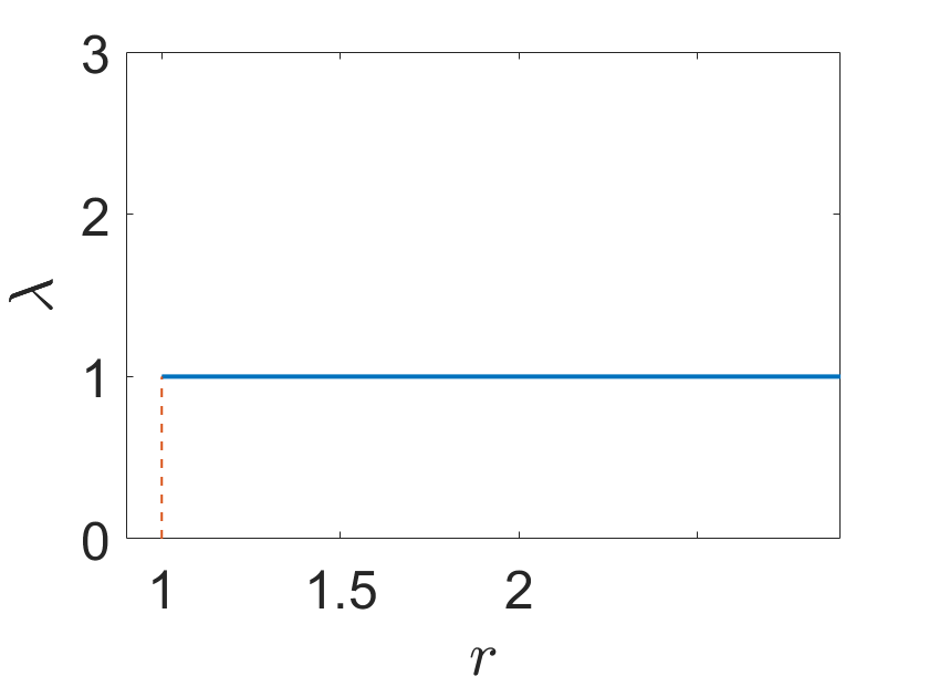
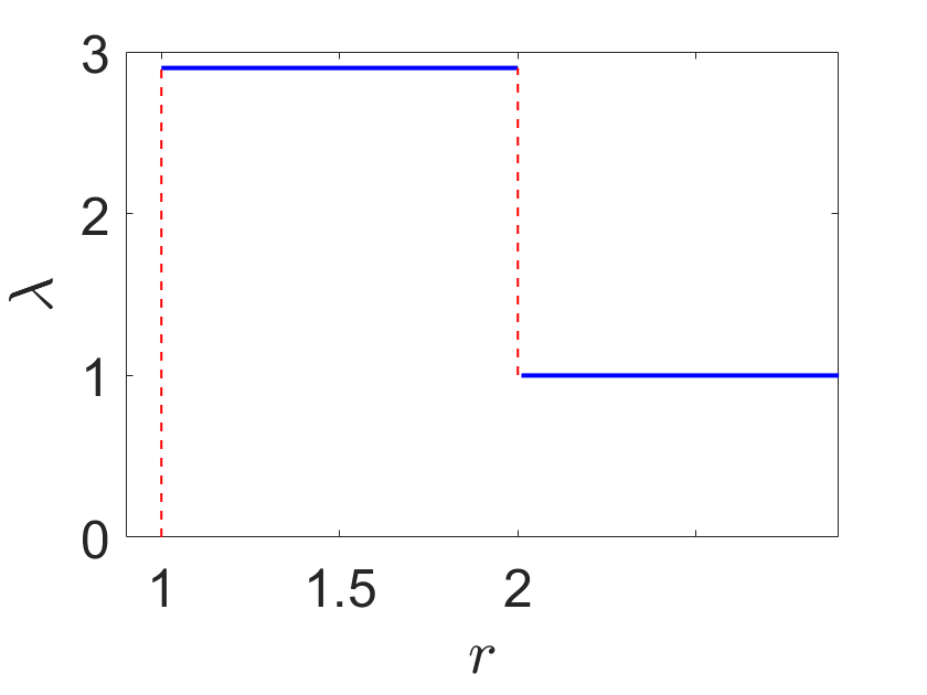
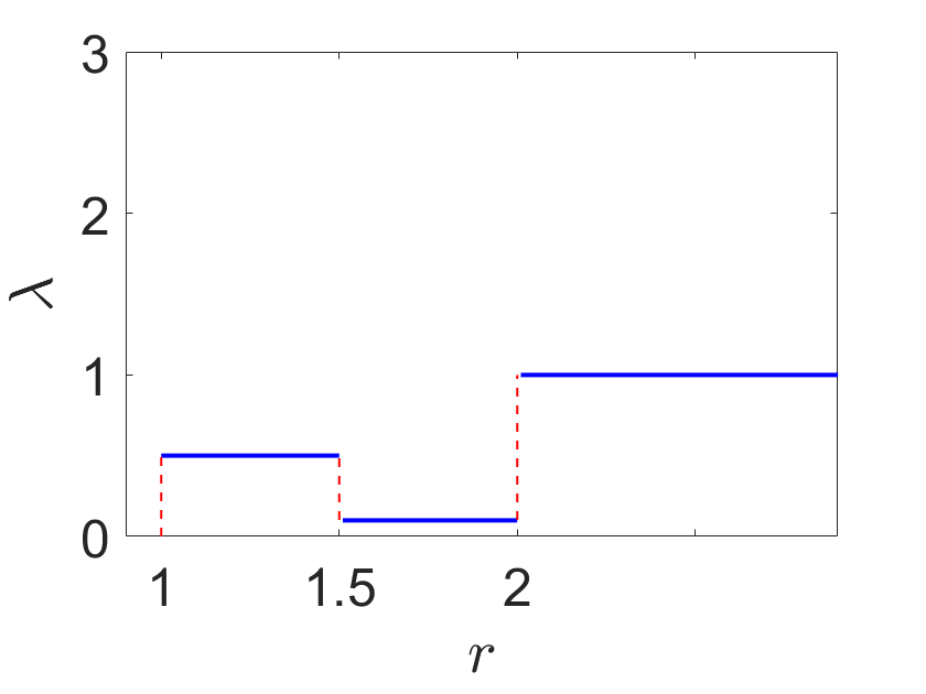
Figure 1: The top row, center row and bottom row denote parameters λ\lambda, μ\mu and ρ\rho, respectively. The left column denotes the case with no layer, the center column denotes the case with 11 cloaking layer, and the right column denotes the case with 22 cloaking layers.
Refer to caption
(a) 0 layer
Refer to caption
(b) 1 layer
Refer to caption
(c) 2 layers
Refer to caption
(d) 0 layer
Refer to caption
(e) 1 layer
Refer to caption
(f) 2 layers
Figure 2: Scatter plots of the elastic scattering coefficients (WnL​LW_{n}^{LL} and WnN​LW_{n}^{NL}) by using the parameters in Figure 1.

In the first example, we consider an incident wave

uinc​(𝒙)=∑n=0T∑m=−nn𝑱n,mL​(𝒙).u^{\mathrm{inc}}(\bm{x})=\sum_{n=0}^{T}\sum_{m=-n}^{n}\bm{J}_{n,m}^{L}(\bm{x}).

Figure 1 shows the computed material parameters with different layers. The parameters are λ=2.9\lambda=2.9, μ=0.7\mu=0.7 and ρ=0.9\rho=0.9 when using one layer, and λ=(0.1,0.5)\lambda=(0.1,0.5), μ=(1.9,0.1)\mu=(1.9,0.1) and ρ=(0.1,1.6)\rho=(0.1,1.6) when using two layers. The elastic scattering coefficients WnL​LW_{n}^{LL} and WnN​LW_{n}^{NL} are shown in Figure 2. It is clear that the elastic scattering coefficients get smaller as the number of layers increases.

Refer to caption
(a) 0 layer
Refer to caption
(b) 1 layer
Refer to caption
(c) 2 layers
Refer to caption
(d) 0 layer
Refer to caption
(e) 1 layer
Refer to caption
(f) 2 layers
Figure 3: Scatter plots of the scattering coefficients (WnL​NW_{n}^{LN} and WnN​NW_{n}^{NN}) by using different parameters.

In the second example, we consider an incident wave

uinc​(𝒙)=∑n=0T∑m=−nn𝑱n,mN​(𝒙).u^{\mathrm{inc}}(\bm{x})=\sum_{n=0}^{T}\sum_{m=-n}^{n}\bm{J}_{n,m}^{N}(\bm{x}).

Through calculation, the material parameters are λ=0.5\lambda=0.5, μ=0.1\mu=0.1 and ρ=2.7\rho=2.7 when using one layer, and λ=(1.9,1.5)\lambda=(1.9,1.5), μ=(1.5,1.1)\mu=(1.5,1.1) and ρ=(1.1,0.6)\rho=(1.1,0.6) when using two layers. Figure 3 presents the computed elastic scattering coefficients with different layers.

In the final example, we consider an incident wave

uinc​(𝒙)=∑n=0T∑m=−nn𝑱n,mM​(𝒙).u^{\mathrm{inc}}(\bm{x})=\sum_{n=0}^{T}\sum_{m=-n}^{n}\bm{J}_{n,m}^{M}(\bm{x}).

The computed material parameters are λ=0.1\lambda=0.1, μ=2.5\mu=2.5 and ρ=1.2\rho=1.2 when using one layer, and λ=(0.1,0.1)\lambda=(0.1,0.1), μ=(1.9,0.1)\mu=(1.9,0.1) and ρ=(1.6,0.1)\rho=(1.6,0.1) when using two layers. Figure 4 presents the computed elastic scattering coefficient WnM​MW_{n}^{MM} with different layers.

Refer to caption
(a) 0 layer
Refer to caption
(b) 1 layer
Refer to caption
(c) 2 layers
Figure 4: Scatter plots of the elastic scattering coefficient WnM​MW_{n}^{MM} by using different parameters.

5 Nearly ESC-Vanishing Structures and Enhancement of the Near-Cloaking

In this section, we are interested in a nearly ESC-vanishing structure of order K∈ℕK\in\mathbb{N} at low frequencies in order to construct an effective near-elastic cloaking device. Precisely, we would like to design (λ,μ,ρ)(\lambda,\mu,\rho) such that

Wnȷ,ȷ′​[λ,μ,ρ,ϵ​ω]=o⁡(ϵ2​K+2),∀ȷ,ȷ′=L,M,N,\displaystyle W^{\jmath,\jmath^{\prime}}_{n}[\lambda,\mu,\rho,\epsilon\omega]=o(\epsilon^{2K+2}),\qquad\forall\,\jmath,\jmath^{\prime}=L,M,N,

for all n≤Kn\leq K and ϵ≤ϵ0\epsilon\leq\epsilon_{0} for some ϵ0∈ℝ+\epsilon_{0}\in\mathbb{R}_{+}. Towards this end, we will first perform a low-frequency asymptotic analysis of the ESC. Then, we will explain the idea of enhancing the capabilities of near-cloaking devices using the concept of nearly ESC-vanishing structures at low-frequencies.

5.1 Low-Frequency Behavior of ESC

Let us first derive an asymptotic expansion of the entries of 𝐑nL,N​[λ,μ,ρ,τ]\mathbf{R}_{n}^{L,N}[\lambda,\mu,\rho,\tau] and 𝐑nM​[λ,μ,ρ,τ]\mathbf{R}_{n}^{M}[\lambda,\mu,\rho,\tau] where τ=ϵ​ω\tau=\epsilon\omega. Towards this end, let us recall the series expansions of the spherical Bessel functions of the first and second kinds (see, e.g., [22, Eqs. 9.39-9.40]),

jn​(τ)=∑k=0∞(−1)k​τn+2​k2kk!1⋅3⋯(2n+2k+1),\displaystyle j_{n}(\tau)=\sum_{k=0}^{\infty}\frac{{(-1)}^{k}\tau^{n+2k}}{2^{k}k!1\cdot 3\cdots(2n+2k+1)},
yn(τ)=−(2​n)!2n​n!∑k=0∞(−1)k​τ2​k−n−12kk!(−2n+1)(−2n+3)⋯(−2n+2k+1).\displaystyle y_{n}(\tau)=-\frac{{(2n)}!}{2^{n}n!}\sum_{k=0}^{\infty}\frac{{(-1)}^{k}\tau^{2k-n-1}}{2^{k}k!(-2n+1)(-2n+3)\cdots(-2n+2k+1)}.

If we use the notation

k!!={k⋅(k−2)⋯3⋅1if​k>0​is odd,k⋅(k−2)⋯4⋅2if​k>0​is even,1if​k=−1,0,k!!=\begin{cases}k\cdot(k-2)\cdots 3\cdot 1&\text{if}\ k>0\ \text{is odd},\\ k\cdot(k-2)\cdots 4\cdot 2&\text{if}\ k>0\ \text{is even},\\ 1&\text{if}\ k=-1,0,\end{cases}

then

(53) jn​(τ)=τn(2​n+1)!!​(1+o⁡(τ)),\displaystyle j_{n}(\tau)=\frac{\tau^{n}}{(2n+1)!!}(1+o(\tau)), for​τ≪1,\displaystyle\text{for}\ \tau\ll 1,
(54) yn​(τ)=((2​n−1)!!)​τ−n−1​(1+o⁡(τ)),\displaystyle y_{n}(\tau)=((2n-1)!!)\tau^{-n-1}(1+o(\tau)), for​τ≫1.\displaystyle\text{for}\ \tau\gg 1.

Based on the behavior of the spherical Bessel functions (53)-(54), the following result holds. Refer to Appendix D for a sketch of the proof.

Lemma 5.1.

Let K∈ℕK\in\mathbb{N} be fixed, n∈ℕn\in\mathbb{N} be such that n≤Kn\leq K, and p,q=1,⋯,4p,q=1,\cdots,4. Then, there exist functions fn,kMf^{M}_{n,k}, gn,kMg^{M}_{n,k}, fn,k,p,qL,Nf^{L,N}_{n,k,p,q}, and gn,k,p,qL,Ng^{L,N}_{n,k,p,q} independent of τ\tau such that, as τ=ϵ​ω→0\tau=\epsilon\omega\to 0,

(55) {(RnM)1,1​[τ]=τn​(∑k=0K−nfn,kM​(λ,μ,ρ)​τ2​k+o⁡(τ2​K−2​n)),(RnM)1,2​[τ]=τ−n−1​(∑k=0K−ngn,kM​(λ,μ,ρ)​τ2​k+o⁡(τ2​K−2​n)),(RnL,N)p,q​[τ]=τn−1​(∑k=0K−nfn,k,p,qL,N​(λ,μ,ρ)​τ2​k+o⁡(τ2​K−2​n)),q=1,2,(RnL,N)p,q​[τ]=τ−n−2​(∑k=0K−ngn,k,p,qL,N​(λ,μ,ρ)​τ2​k+o⁡(τ2​K−2​n)),q=3,4.\displaystyle\begin{cases}\displaystyle{(R^{M}_{n})}_{1,1}[\tau]=\tau^{n}\left(\sum_{k=0}^{K-n}f^{M}_{n,k}(\lambda,\mu,\rho)\tau^{2k}+o(\tau^{2K-2n})\right),\\ \displaystyle{(R^{M}_{n})}_{1,2}[\tau]=\tau^{-n-1}\left(\sum_{k=0}^{K-n}g^{M}_{n,k}(\lambda,\mu,\rho)\tau^{2k}+o(\tau^{2K-2n})\right),\\ \displaystyle(R_{n}^{L,N})_{p,q}[\tau]=\tau^{n-1}\left(\sum_{k=0}^{K-n}f^{L,N}_{n,k,p,q}(\lambda,\mu,\rho)\tau^{2k}+o(\tau^{2K-2n})\right),&q=1,2,\\ \displaystyle(R_{n}^{L,N})_{p,q}[\tau]=\tau^{-n-2}\left(\sum_{k=0}^{K-n}g^{L,N}_{n,k,p,q}(\lambda,\mu,\rho)\tau^{2k}+o(\tau^{2K-2n})\right),&q=3,4.\end{cases}

Let us assume that for any (λ,μ,ρ)(\lambda,\mu,\rho),

gn,0M​(λ,μ,ρ)≠0andgn,0,p,qL,N​(λ,μ,ρ)≠0,∀p,q=3,4,\displaystyle g^{M}_{n,0}(\lambda,\mu,\rho)\neq 0\quad\text{and}\quad g^{L,N}_{n,0,p,q}(\lambda,\mu,\rho)\neq 0,\quad\forall p,q=3,4,

where the functions gn,0Mg^{M}_{n,0} and gn,0,k,lL,Ng^{L,N}_{n,0,k,l} are given in Lemma 5.1. Then, the following result can be easily verified using simple algebra.

Theorem 5.2.

Let K∈ℕK\in\mathbb{N} be fixed and n∈ℕn\in\mathbb{N} be such that n≤Kn\leq K. Then, there exist functions Wn,kȷ,ȷ′​[λ,μ,ρ]W_{n,k}^{\jmath,\jmath^{\prime}}[\lambda,\mu,\rho] and Wn,kM,M​[λ,μ,ρ]W_{n,k}^{M,M}[\lambda,\mu,\rho] independent of τ\tau for 0≤k≤K−n0\leq k\leq K-n such that, as τ=ϵ​ω→0\tau=\epsilon\omega\to 0,

Wnȷ,ȷ′​[λ,μ,ρ,τ]=τ2​n​∑k=0K−nWn,kȷ,ȷ′​[λ,μ,ρ]​τ2​p+o⁡(τ2​K),\displaystyle\displaystyle W_{n}^{\jmath,\jmath^{\prime}}[\lambda,\mu,\rho,\tau]=\tau^{2n}\sum_{k=0}^{K-n}W_{n,k}^{\jmath,\jmath^{\prime}}[\lambda,\mu,\rho]\tau^{2p}+o(\tau^{2K}),
WnM,M​[λ,μ,ρ,τ]=τ2​n​∑p=0K−nWn,kM,M​[λ,μ,ρ]​τ2​k+o⁡(τ2​K),ȷ,ȷ′=L,N.\displaystyle\displaystyle W_{n}^{M,M}[\lambda,\mu,\rho,\tau]=\tau^{2n}\sum_{p=0}^{K-n}W_{n,k}^{M,M}[\lambda,\mu,\rho]\tau^{2k}+o(\tau^{2K}),\qquad\jmath,\jmath^{\prime}=L,N.

Notice that, thanks to Lemma 3.2, we have

|Wnȷ,ȷ′​[λ,μ,ρ,ϵ​ω]|≤C2​n−2n2​n−2​ϵ2​n−2,∀ȷ,ȷ′=L,Norȷ=ȷ′=M,\displaystyle\Big|W_{n}^{\jmath,\jmath^{\prime}}[\lambda,\mu,\rho,\epsilon\omega]\Big|\leq\frac{C^{2n-2}}{n^{2n-2}}\epsilon^{2n-2},\quad\forall\jmath,\jmath^{\prime}=L,N\quad\text{or}\quad\jmath=\jmath^{\prime}=M,

for all n∈ℕn\in\mathbb{N}. Hence, if we can find a structure (λ,μ,ρ)(\lambda,\mu,\rho) at low frequencies such that the coefficients

Wn,kL,L=Wn,kN,L=Wn,kN,N=Wn,kL,N=Wn,kM,M=0,\displaystyle W_{n,k}^{L,L}=W_{n,k}^{N,L}=W_{n,k}^{N,N}=W_{n,k}^{L,N}=W_{n,k}^{M,M}=0,

for all 0≤n≤K0\leq n\leq K and 0≤k≤(K−n)0\leq k\leq(K-n), then

Wnȷ,ȷ′​[λ,μ,ρ,ϵ​ω]=o⁡(ϵ2​K−2),ȷ,ȷ′=L,N,\displaystyle W_{n}^{\jmath,\jmath^{\prime}}[\lambda,\mu,\rho,\epsilon\omega]=o(\epsilon^{2K-2}),\quad\jmath,\jmath^{\prime}=L,N,
WnM,M​[λ,μ,ρ,ϵ​ω]=o⁡(ϵ2​K−2),\displaystyle W_{n}^{M,M}[\lambda,\mu,\rho,\epsilon\omega]=o(\epsilon^{2K-2}),

for all ϵ≤ϵ0\epsilon\leq\epsilon_{0} for some ϵ0∈ℝ+\epsilon_{0}\in\mathbb{R}_{+} thanks to Theorem 5.2. In that case, the far-field signature of the core is also of order o⁡(ϵ2​K−2)o(\epsilon^{2K-2}) for all ϵ≤ϵ0\epsilon\leq\epsilon_{0}. For example, consider an incident wave 𝐪​eι​κS​𝒙⋅𝐝\mathbf{q}e^{\iota\kappa_{S}{{\itbf x}}\cdot{{\bf d}}} given by (20). Then, the scattering amplitudes, defined in (28), satisfy

𝒖P∞​[λ,μ,ρ,ϵ​ω]=o⁡(ϵ2​K−2)and𝒖S∞​[λ,μ,ρ,ϵ​ω]=o⁡(ϵ2​K−2),\displaystyle{{\itbf u}}^{\infty}_{P}[\lambda,\mu,\rho,\epsilon\omega]=o(\epsilon^{2K-2})\quad\text{and}\quad{{\itbf u}}^{\infty}_{S}[\lambda,\mu,\rho,\epsilon\omega]=o(\epsilon^{2K-2}),

for all ϵ≤ϵ0\epsilon\leq\epsilon_{0} thanks to Proposition 3.4. Hence, the application of the nearly ESC-vanishing structure can effectively reduce the visibility of the scattering signature of an object.

5.2 Enhancement of Near-Cloaking in Elasticity

In this section, we combine the transformation-elastodynamic and the ESC-vanishing structures to enhance the performance of near-elastic cloaking procedures. Let us first briefly review the transformation-elastodynamics and recall the following Lemma from [16].

Lemma 5.3.

Let 𝐱~=(x~1,x~2,x~3)=ℱ:ℝ3→ℝ3\widetilde{{{\itbf x}}}=(\widetilde{x}_{1},\widetilde{x}_{2},\widetilde{x}_{3})=\mathcal{F}:\mathbb{R}^{3}\to\mathbb{R}^{3} be an orientation-preserving bi-Lipschitz continuous diffeomorphism such that ℱ=ℐ\mathcal{F}=\mathcal{I} for |𝐱||{{\itbf x}}| large enough, where ℐ\mathcal{I} is the identity map. Then, 𝐮∈H1​(ℝ3){{\itbf u}}\in H^{1}(\mathbb{R}^{3}) is a solution to

{∇⋅(ℭ:∇𝒖)+ω2​ρ​𝒖=0,in ​ℝ3,𝒖−𝒖incsatisfies Kupradze’s radiation condition,\begin{cases}\nabla\cdot(\mathfrak{C}:\nabla{{\itbf u}})+\omega^{2}\rho{{\itbf u}}=0,\quad\text{in }\,\mathbb{R}^{3},\\ {{\itbf u}}-{{\itbf u}}^{\rm inc}\quad\text{satisfies Kupradze's radiation condition},\end{cases}

if and only if 𝐮~​(𝐲~)=𝐮∘ℱ−1​(𝐲~)∈H1​(ℝ3)\widetilde{{{\itbf u}}}(\widetilde{{{\itbf y}}})={{\itbf u}}\circ\mathcal{F}^{-1}(\widetilde{{{\itbf y}}})\in H^{1}(\mathbb{R}^{3}) is a solution to

{∇~⋅(ℭ~:∇~​𝒖~)+ω2​ρ~​𝒖~=0,in ​ℝ3,𝒖~−𝒖~inc satisfies Kupradze’s radiation condition,\begin{cases}\widetilde{\nabla}\cdot(\widetilde{\mathfrak{C}}:\widetilde{\nabla}\widetilde{{{\itbf u}}})+\omega^{2}\widetilde{\rho}\widetilde{{{\itbf u}}}=0,\quad\text{in }\,\mathbb{R}^{3},\\ \widetilde{{{\itbf u}}}-\widetilde{{{\itbf u}}}^{\rm inc}\quad\text{ satisfies Kupradze's radiation condition},\end{cases}

where ∇~:=∇𝐱~\widetilde{\nabla}:=\nabla_{\widetilde{{{\itbf x}}}} and 𝐮~inc:=𝐮inc​(ℱ−1)​(𝐲~)\widetilde{{{\itbf u}}}^{\rm inc}:={{\itbf u}}^{\rm inc}(\mathcal{F}^{-1})(\widetilde{{{\itbf y}}}). Here, the transformed stiffness tensor and the volume density are given by ℭ~=(C~i​j​k​l​(x~))i,j,k,l=13=ℱ∗​ℭ\widetilde{\mathfrak{C}}=\left(\widetilde{C}_{ijkl}(\widetilde{x})\right)_{i,j,k,l=1}^{3}=\mathcal{F}_{\ast}\mathfrak{C} with 𝐌=(∂x~i/∂xj)i,j=13\mathbf{M}={\left({\partial\widetilde{x}_{i}}/{\partial{x}_{j}}\right)}^{3}_{i,j=1} and

C~i​j​k​l​(x~)=1det(𝐌)​(∑p,q=13Ci​p​k​q​∂x~j∂xp​∂x~l∂xq)|𝒙=ℱ−1​(𝒚~),\displaystyle\widetilde{C}_{ijkl}(\widetilde{x})=\frac{1}{\det(\mathbf{M})}\left.\left(\sum_{p,q=1}^{3}C_{ipkq}\frac{\partial\widetilde{x}_{j}}{\partial{x}_{p}}\frac{\partial\widetilde{x}_{l}}{\partial x_{q}}\right)\right|_{{{\itbf x}}=\mathcal{F}^{-1}(\widetilde{{{\itbf y}}})},
ρ~=ℱ∗​ρ=(ρdet(𝐌))|𝒙=ℱ−1​(𝒚~).\displaystyle\widetilde{\rho}=\mathcal{F}_{\ast}\rho=\left.\left(\frac{\rho}{\det(\mathbf{M})}\right)\right|_{{{\itbf x}}=\mathcal{F}^{-1}(\widetilde{{{\itbf y}}})}.

Hence,

𝒖α∞[ℭ,ρ,ω]=𝒖~α∞[ℱ∗ℭ,ℱ∗ρ,ω],α=P,S.{{\itbf u}}^{\infty}_{\alpha}[\mathfrak{C},\rho,\omega]=\widetilde{{{\itbf u}}}^{\infty}_{\alpha}[\mathcal{F}_{\ast}\mathfrak{C},\mathcal{F}_{\ast}\rho,\omega],\qquad\alpha=P,S.

We would like to point out that in Lemma 5.3, the transformed elastic tensor C~\widetilde{C} does not possess the minor symmetry required for an elastic tensor, namely C~i​j​k​l\widetilde{C}_{ijkl} lacks the (i,j)(i,j)-symmetry. This poses a significant challenge for the practical value of the transformation-elastodynamics-based cloaks. In fact, it was pointed by Milton et al. [21] that the invariance of the Lamé system can be achieved only if one relaxes the minor symmetry of the transformed elastic tensor. In order to overcome this practical challenge, Norris and Shuvalov [25] and Parnell [28] have explored the elastic cloaking by using Cosserat material or by employing non-linear pre-stress in a neo-Hookean elastomeric material. Designs of transformation-elastodynamics-based Cosserat elastic cloaks without the minor symmetry have been numerically studied in [8, 13]. We refer Remark 2.1 in [16] for more relevant discussions on this point.

In order to apply transformation-elastodynamics, we need to find the scattering amplitudes corresponding to the material parameters beforehand. Towards this end, we introduce the scaling function

ψ1/ϵ:ℝ3→ℝ3,𝒙↦𝒙/ϵ,\psi_{{1}/{\epsilon}}:\mathbb{R}^{3}\to\mathbb{R}^{3},\quad{{\itbf x}}\mapsto{{{\itbf x}}}/{\epsilon},

for transforming the small parameter ϵ\epsilon. Our aim is to obtain the following relation between two scattering amplitudes corresponding to different scaled material parameters and frequency. Consider 𝒖{{\itbf u}} as a solution to

{∇⋅(ℭ:∇𝒖(𝒙))+ω2ρ𝒖(x)=𝟎,for𝒙∈ℝ3∖Bϵ​(𝟎)¯,𝐓⁡[𝒖]​(𝒙)=0,on​∂Bϵ​(𝟎),(𝒖−𝒖inc)​(𝒙)satisfies the Kupradze’s radiation condition,\begin{cases}\nabla\cdot(\mathfrak{C}:\nabla{{\itbf u}}({{\itbf x}}))+\omega^{2}\rho{{\itbf u}}(x)=\mathbf{0},\quad\text{for}\ {{\itbf x}}\in\mathbb{R}^{3}\setminus\overline{B_{\epsilon}(\mathbf{0})},\\ \mathbf{T}[{{\itbf u}}]({{\itbf x}})=0,\quad\text{on}\ \partial B_{\epsilon}(\mathbf{0}),\\ ({{\itbf u}}-{{\itbf u}}^{\rm inc})({{\itbf x}})\quad\text{satisfies the Kupradze's radiation condition},\end{cases}

where the incident wave is 𝒖inc=𝐪​eι​κS​𝒙⋅𝐝{{\itbf u}}^{\rm inc}=\mathbf{q}e^{\iota\kappa_{S}{{{\itbf x}}\cdot{{\bf d}}}} given in (20). Here, Bϵ​(𝟎)B_{\epsilon}(\mathbf{0}) denotes the ball centered at origin and of radius ϵ\epsilon. Let 𝒚=𝒙/ϵ{{\itbf y}}={{{\itbf x}}}/{\epsilon} and define

𝒖~​(𝒚):=(𝒖∘ψ1/ϵ−1)​(𝒚)=(𝒖∘ψϵ)​(𝒚),\displaystyle\widetilde{{{\itbf u}}}({{\itbf y}}):=\left({{\itbf u}}\circ\psi_{{1}/{\epsilon}}^{-1}\right)({{\itbf y}})=({{\itbf u}}\circ\psi_{\epsilon})({{\itbf y}}),
𝒖~inc​(𝒚):=(𝒖inc∘ψ1/ϵ−1)​(𝒚)=(𝒖inc∘ψϵ)​(𝒚),\displaystyle\widetilde{{{\itbf u}}}^{\rm inc}({{\itbf y}}):=\left({{\itbf u}}^{\rm inc}\circ\psi_{{1}/{\epsilon}}^{-1}\right)({{\itbf y}})=({{\itbf u}}^{\rm inc}\circ\psi_{\epsilon})({{\itbf y}}),
𝐓⁡[𝒖~]​(𝒚):=λ⁡(∇~⋅𝒖~​(𝒚))​𝝂~+μ⁡(∇~​𝒖~​(𝒚)+∇~​𝒖~⊤​(𝒚))​𝝂~.\displaystyle\mathbf{T}[\widetilde{{{\itbf u}}}]({{\itbf y}}):=\lambda\big(\widetilde{\nabla}\cdot\widetilde{{{\itbf u}}}({{\itbf y}})\big)\widetilde{\bm{\nu}}+\mu\big(\widetilde{\nabla}\widetilde{{{\itbf u}}}({{\itbf y}})+\widetilde{\nabla}\widetilde{{{\itbf u}}}^{\top}({{\itbf y}})\big)\widetilde{\bm{\nu}}.

Then, the scattering amplitudes are given by

(𝒖−𝒖inc)​(𝒙)∼eι​κP​|𝒙|κP​|𝒙|​𝒖P∞​[ℭ∘ψ1/ϵ,ρ∘ψ1/ϵ,ϵ​ω]​(𝒙^)\displaystyle({{\itbf u}}-{{\itbf u}}^{\rm inc})({{\itbf x}})\thicksim\frac{e^{\iota\kappa_{P}|{{\itbf x}}|}}{\kappa_{P}|{{\itbf x}}|}{{\itbf u}}^{\infty}_{P}[\mathfrak{C}\circ\psi_{{1}/{\epsilon}},\rho\circ\psi_{{1}/{\epsilon}},\epsilon\omega](\hat{{{\itbf x}}})
+eι​κS​|𝒙|κS​|𝒙|​𝒖S∞​[ℭ∘ψ1/ϵ,ρ∘ψ1/ϵ,ϵ​ω]​(𝒙^),as ​|𝒙|→∞,\displaystyle\phantom{({{\itbf u}}-{{\itbf u}}^{\rm inc})({{\itbf x}})\thicksim}+\frac{e^{\iota\kappa_{S}|{{\itbf x}}|}}{\kappa_{S}|{{\itbf x}}|}{{\itbf u}}^{\infty}_{S}[\mathfrak{C}\circ\psi_{{1}/{\epsilon}},\rho\circ\psi_{{1}/{\epsilon}},\epsilon\omega]({\hat{{{\itbf x}}}}),\quad\text{as }\,|{{\itbf x}}|\to\infty,
(𝒖~−𝒖~inc)​(𝒚)∼eι​κP​|𝒚|κP​|𝒚|​𝒖P∞​[ℭ,ρ,ϵ​ω]​(𝒚^)+eι​κS​|𝒚|κS​|𝒚|​𝒖S∞​[ℭ,ρ,ϵ​ω]​(𝒚^),as ​|𝒚|→∞.\displaystyle(\widetilde{{{\itbf u}}}-\widetilde{{{\itbf u}}}^{\rm inc})({{\itbf y}})\thicksim\frac{e^{\iota\kappa_{P}|{{\itbf y}}|}}{\kappa_{P}|{{\itbf y}}|}{{\itbf u}}^{\infty}_{P}[\mathfrak{C},\rho,\epsilon\omega]({\hat{{{\itbf y}}}})+\frac{e^{\iota\kappa_{S}|{{\itbf y}}|}}{\kappa_{S}|{{\itbf y}}|}{{\itbf u}}^{\infty}_{S}[\mathfrak{C},\rho,\epsilon\omega]({\hat{{{\itbf y}}}}),\,\,\text{as }\,|{{\itbf y}}|\to\infty.

Since (𝒖−𝒖inc)​(𝒙){({{\itbf u}}-{{\itbf u}}^{\rm inc})({{\itbf x}})} and (𝒖~−𝒖~inc)​(𝒚){(\widetilde{{{\itbf u}}}-\widetilde{{{\itbf u}}}^{\rm inc})({{\itbf y}})} should coincide, we have

𝒖α∞[ℭ∘ψ1/ϵ𝒙,ρ∘ψ1/ϵ(𝒙),ω]=𝒖α∞[ℭ,ρ,ϵω],α=P,S.{{\itbf u}}^{\infty}_{\alpha}[\mathfrak{C}\circ\psi_{{1}/{\epsilon}}{{\itbf x}},\rho\circ\psi_{{1}/{\epsilon}}({{\itbf x}}),\omega]={{\itbf u}}^{\infty}_{\alpha}[\mathfrak{C},\rho,\epsilon\omega],\qquad\alpha=P,S.

Suppose that (λ,μ,ρ)(\lambda,\mu,\rho) is an ESC-vanishing structure of order KK at low frequencies ϵ​ω\epsilon\omega for all ϵ<ϵ0\epsilon<\epsilon_{0} for some ϵ0\epsilon_{0}. Then, we have

(56) 𝒖P∞​[ℭ∘ψ1/ϵ​(𝒙),ρ∘ψ1/ϵ​(𝒙),ω]=o⁡(ϵ2​K−2)=𝒖S∞​[ℭ∘ψ1/ϵ​𝒙,ρ∘ψ1/ϵ​𝒙,ω],\displaystyle\itbf{{\displaystyle u}}^{\infty}_{P}[\mathfrak{C}\circ\psi_{{1}/{\epsilon}}{({{\itbf x}})},\rho\circ\psi_{{1}/{\epsilon}}({{\itbf x}}),\omega]=o(\epsilon^{2K-2})={{\itbf u}}^{\infty}_{S}[\mathfrak{C}\circ\psi_{{1}/{\epsilon}}{{\itbf x}},\rho\circ\psi_{{1}/{\epsilon}}{{\itbf x}},\omega],

and the diffeomorphism ℱϵ\mathcal{F}_{\epsilon} is defined by

ℱϵ​(𝒙):={𝒙,for ​|𝒙|≥2,(3−4​ϵ2​(1−ϵ)+|𝒙|4​(1−ϵ))​𝒙|𝒙|,for ​ 2​ϵ≤|𝒙|≤2,(12+|𝒙|2​ϵ)​𝒙|𝒙|,for ​ϵ≤|𝒙|≤2​ϵ,𝒙ϵ,for ​|𝒙|≤ϵ.\mathcal{F}_{\epsilon}({{\itbf x}}):=\begin{cases}{{\itbf x}},&\text{for }\,|{{\itbf x}}|\geq 2,\\ \displaystyle\left(\frac{3-4\epsilon}{2(1-\epsilon)}+\frac{|{{\itbf x}}|}{4(1-\epsilon)}\right){\frac{{{\itbf x}}}{|{{\itbf x}}|}},&\text{for }\,2\epsilon\leq|{{\itbf x}}|\leq 2,\\ \displaystyle\left(\frac{1}{2}+\frac{|{{\itbf x}}|}{2\epsilon}\right)\frac{{{\itbf x}}}{|{{\itbf x}}|},&\text{for }\,\epsilon\leq|{{\itbf x}}|\leq 2\epsilon,\\ \displaystyle\frac{{{\itbf x}}}{\epsilon},&\text{for }\,|{{\itbf x}}|\leq\epsilon.\end{cases}

Therefore, estimate (56), Proposition 5.2, and Lemma 5.3 yield the following key result of this paper.

Theorem 5.4.

If (λ,μ,ρ)(\lambda,\mu,\rho) is a nearly ESC-vanishing structure of order KK at low frequencies then there exists ϵ0∈ℝ+\epsilon_{0}\in\mathbb{R}_{+} such that, for all ϵ≤ϵ0\epsilon\leq\epsilon_{0},

𝒖∞​[(ℱϵ)∗​(ℭ∘ψ1/ϵ​(𝒙)),(ℱϵ)∗​(ρ∘ψ1/ϵ​(𝒙)),ω]=o⁡(ϵ2​K−2).\displaystyle{{\itbf u}}^{\infty}\left[(\mathcal{F}_{\epsilon})_{\ast}\left(\mathfrak{C}\circ\psi_{{1}/{\epsilon}}({{\itbf x}})\right),(\mathcal{F}_{\epsilon})_{\ast}\left(\rho\circ\psi_{{1}/{\epsilon}}({{\itbf x}})\right),\omega\right]=o(\epsilon^{2K-2}).

6 Conclusion

A new method for the design of a near-cloaking structure has been presented at a fixed frequency that enhanced the invisibility effect based on the scheme of vanishing scattering coefficients to elastic scattering problems in three-dimensions. We have achieved a cloaking effect for an arbitrary elastic object inside the cloaked region with approximately zero scattering amplitudes. Such a cloaking device is obtained by using the transformation-elastodynamics approach of a multi-layered inclusion with a traction-free boundary condition. The cloaking effect for the Lamé system is significantly enhanced by the proposed near cloaking structures.

Acknowledgement

The research of H Liu was supported by the startup fund from City University of Hong Kong and the Hong Kong RGC General Research Fund ( projects 12302017, 12301218 and 12302919). The research of X Wang was supported by the Hong Kong Scholars Program grant XJ2019005 and the NSFC grant (11971133 and 12001140).

Appendix A Proof of Theorem 3.3

Let us first introduce some notation. For all functions 𝒗,𝒘∈H3/2​(D)3{{\itbf v}},{{\itbf w}}\in H^{3/2}(D)^{3} and a,b∈ℝa,b\in\mathbb{R}, we define the quadratic form

⟨𝒗,𝒘⟩Da,b:=∫D[a(∇⋅𝒗)(∇⋅𝒘)+b2(∇𝒗+∇𝒗⊤):(∇𝒘+∇𝒘⊤)]d𝒙.\displaystyle\langle{{\itbf v}},{{\itbf w}}\rangle^{a,b}_{D}:=\int_{D}\left[a(\nabla\cdot{{\itbf v}})(\nabla\cdot{{\itbf w}})+\frac{b}{2}(\nabla{{\itbf v}}+\nabla{{\itbf v}}^{\top}):(\nabla{{\itbf w}}+\nabla{{\itbf w}}^{\top})\right]d{{\itbf x}}.

Here, by slight abuse of notation, we use ‘::’ for denoting the matrix contraction, i.e., 𝐀:𝐁:=∑i,jai​j​bi​j\mathbf{A}:\mathbf{B}:=\sum_{i,j}a_{ij}b_{ij} for all matrices 𝐀=(ai​j)\mathbf{A}=(a_{ij}) and 𝐁=(bi​j)\mathbf{B}=(b_{ij}) having the same dimensions. From the definition, we know that

(57) ∫∂D𝒗⋅𝐓a,b​[𝒘]​𝑑σ​(𝒙)=∫D𝒗⋅ℒa,b​[𝒘]​𝑑𝒙+⟨𝒗,𝒘⟩Da,b,\int_{\partial D}{{\itbf v}}\cdot\mathbf{T}_{a,b}[{{\itbf w}}]d\sigma({{\itbf x}})=\int_{D}{{\itbf v}}\cdot\mathcal{L}_{a,b}[{{\itbf w}}]d{{\itbf x}}+\langle{{\itbf v}},{{\itbf w}}\rangle^{a,b}_{D},

where 𝐓a,b\mathbf{T}_{a,b} is the surface traction defined in terms of parameters a,ba,b. If 𝒘{{\itbf w}} solves the Lamé system ℒa,b​[𝒘]+c​ω2​𝒘=𝟎\mathcal{L}_{a,b}[{{\itbf w}}]+c\omega^{2}{{\itbf w}}=\mathbf{0}, for some c∈ℝ+c\in\mathbb{R}_{+}, then

∫∂D𝒗⋅𝐓a,b[𝒘]dσ(𝒙)=−cω2∫∂D𝒗⋅𝒘d𝒙+⟨𝒗,𝒘⟩Da,b,\displaystyle\int_{\partial D}{{\itbf v}}\cdot\mathbf{T}_{a,b}[{{\itbf w}}]d\sigma({{\itbf x}})=-c\omega^{2}\int_{\partial D}{{\itbf v}}\cdot{{\itbf w}}d{{\itbf x}}+\langle{{\itbf v}},{{\itbf w}}\rangle^{a,b}_{D},

and hence from (57), we have

(58) ∫∂D𝒗⋅𝐓a,b​[𝒘]​𝑑σ​(𝒙)=\displaystyle\int_{\partial D}{{\itbf v}}\cdot\mathbf{T}_{a,b}[{{\itbf w}}]d\sigma({{\itbf x}})= ∫∂D𝐓a,b​[𝒗]⋅𝒘​𝑑σ​(𝒙)−c​ω2​∫∂D𝒗⋅𝒘​𝑑𝒙−∫Dℒa,b​[𝒗]⋅𝒘​𝑑𝒙.\displaystyle\int_{\partial D}\mathbf{T}_{a,b}[{{\itbf v}}]\cdot{{\itbf w}}d\sigma({{\itbf x}})-c\omega^{2}\int_{\partial D}{{\itbf v}}\cdot{{\itbf w}}d{{\itbf x}}-\int_{D}\mathcal{L}_{a,b}[{{\itbf v}}]\cdot{{\itbf w}}d{{\itbf x}}.

In addition, if 𝒗{{\itbf v}} is a solution of ℒa,b​[𝒗]+c​ω2​𝒗=𝟎\mathcal{L}_{a,b}[{{\itbf v}}]+c\omega^{2}{{\itbf v}}=\mathbf{0} then

(59) ∫∂D𝒗⋅𝐓a,b​[𝒘]​𝑑σ​(𝒙)=∫∂D𝐓a,b​[𝒗]⋅𝒘​𝑑σ​(𝒙).\int_{\partial D}{{\itbf v}}\cdot\mathbf{T}_{a,b}[{{\itbf w}}]d\sigma({{\itbf x}})=\int_{\partial D}\mathbf{T}_{a,b}[{{\itbf v}}]\cdot{{\itbf w}}d\sigma({{\itbf x}}).

Henceforth, we use the notation

{ηL:=μ0μ1−μ0,η~L:=μ1μ1−μ0,ηM=ηN:=3​λ0+2​μ03​(λ1−λ0)+2​(μ1−μ0),η~M=η~N:=3​λ1+2​μ13​(λ1−λ0)+2​(μ1−μ0).\begin{cases}\displaystyle\eta_{L}:=\frac{\mu_{0}}{\mu_{1}-\mu_{0}},\\ \displaystyle\widetilde{\eta}_{L}:=\frac{\mu_{1}}{\mu_{1}-\mu_{0}},\\ \displaystyle\eta_{M}=\eta_{N}:=\frac{3\lambda_{0}+2\mu_{0}}{3(\lambda_{1}-\lambda_{0})+2(\mu_{1}-\mu_{0})},\\ \displaystyle\widetilde{\eta}_{M}=\widetilde{\eta}_{N}:=\frac{3\lambda_{1}+2\mu_{1}}{3(\lambda_{1}-\lambda_{0})+2(\mu_{1}-\mu_{0})}.\end{cases}

Let (𝝋n​mȷ,𝝍n​mȷ)({\bm{\varphi}}_{nm}^{\jmath},{\bm{\psi}}_{nm}^{\jmath}) and (𝝋k​lȷ′,𝝍k​lȷ′)({\bm{\varphi}}_{kl}^{\jmath^{\prime}},{\bm{\psi}}_{kl}^{\jmath^{\prime}}) be, respectively, the solutions to

(60) 𝒮~Dω​[𝝋n​mȷ]−𝒮Dω​[𝝍n​mȷ]=𝐉n​mȷ|∂D,𝐓~​[𝒮~Dω​[𝝋n​mȷ]]|−−𝐓⁡[𝒮Dω​[𝝍n​mȷ]]|+=𝐓⁡[𝐉n​mȷ]|∂D,\displaystyle\begin{aligned} &\displaystyle\widetilde{\mathcal{S}}^{\omega}_{D}[{\bm{\varphi}}_{nm}^{\jmath}]-\mathcal{S}^{\omega}_{D}[{\bm{\psi}}_{nm}^{\jmath}]=\mathbf{J}^{\jmath}_{nm}\big|_{\partial D},\\ &\displaystyle\widetilde{\mathbf{T}}\big[\widetilde{\mathcal{S}}^{\omega}_{D}[{\bm{\varphi}}_{nm}^{\jmath}]\big]\Big|_{-}-\mathbf{T}\left[\mathcal{S}^{\omega}_{D}[{\bm{\psi}}_{nm}^{\jmath}]\right]\Big|_{+}=\displaystyle\mathbf{T}\left[\mathbf{J}^{\jmath}_{nm}\right]\Big|_{\partial D},\end{aligned}

and

(61) 𝒮~Dω​[𝝋k​lȷ′]−𝒮Dω​[𝝍k​lȷ′]=𝐉k​lȷ′|∂D,𝐓~​[𝒮~Dω​[𝝋k​lȷ′]]|−−𝐓⁡[𝒮Dω​[𝝍k​lȷ′]]|+=𝐓⁡[𝐉k​lȷ′]|∂D.\displaystyle\begin{aligned} &\displaystyle\widetilde{\mathcal{S}}^{\omega}_{D}[{\bm{\varphi}}_{kl}^{\jmath^{\prime}}]-\mathcal{S}^{\omega}_{D}[{\bm{\psi}}_{kl}^{\jmath^{\prime}}]=\mathbf{J}^{\jmath^{\prime}}_{kl}\big|_{\partial D},\\ &\displaystyle\widetilde{\mathbf{T}}\left[\widetilde{\mathcal{S}}^{\omega}_{D}[{\bm{\varphi}}_{kl}^{\jmath^{\prime}}]\right]\Big|_{-}-\mathbf{T}\left[\mathcal{S}^{\omega}_{D}[{\bm{\psi}}_{kl}^{\jmath^{\prime}}]\right]\Big|_{+}=\displaystyle\mathbf{T}\left[\mathbf{J}^{\jmath^{\prime}}_{kl}\right]\Big|_{\partial D}.\end{aligned}

Thanks to jump conditions (10), the scattering coefficients W(n,m),(k,l)ȷ,ȷ′W_{(n,m),(k,l)}^{\jmath,\jmath^{\prime}} can be expressed as

W(n,m),(k,l)ȷ,ȷ′=\displaystyle W_{(n,m),(k,l)}^{\jmath,\jmath^{\prime}}= ∫∂D𝐉n​mȷ¯⋅𝝋k​lȷ′​𝑑σ​(𝒙)\displaystyle\displaystyle\int_{\partial D}\overline{\mathbf{J}_{nm}^{\jmath}}\cdot{\bm{\varphi}}_{kl}^{\jmath^{\prime}}d\sigma({{\itbf x}})
(62) =\displaystyle= ∫∂D𝐉n​mȷ¯⋅[𝐓⁡[𝒮Dω​[𝝋k​lȷ′]]|+−𝐓⁡[𝒮Dω​[𝝋k​lȷ′]]|−]​𝑑σ​(𝒙).\displaystyle\displaystyle\int_{\partial D}\overline{\mathbf{J}_{nm}^{\jmath}}\cdot\left[{\mathbf{T}\left[\mathcal{S}^{\omega}_{D}[{\bm{\varphi}}^{\jmath^{\prime}}_{kl}]\right]}\Big|_{+}-{\mathbf{T}\left[\mathcal{S}^{\omega}_{D}[{\bm{\varphi}}^{\jmath^{\prime}}_{kl}]\right]}\Big|_{-}\right]d\sigma({{\itbf x}}).

Using (61) in (62) and then invoking (58)-(59), one gets

W(n,m),(k,l)ȷ,ȷ′=\displaystyle W_{(n,m),(k,l)}^{\jmath,\jmath^{\prime}}= −∫∂D𝐉n​mȷ¯⋅𝐓[𝐉k​lȷ′]dσ(𝒙)\displaystyle-\int_{\partial D}\overline{\mathbf{J}_{nm}^{\jmath}}\cdot\mathbf{T}\left[\mathbf{J}_{kl}^{\jmath^{\prime}}\right]d\sigma({{\itbf x}})
+∫∂D𝐉n​mȷ¯⋅[𝐓~[𝒮~Dω[𝝍k​lȷ′]]|−−𝐓[𝒮Dω[𝝋k​lȷ′]]|+]dσ(𝒙),\displaystyle+\int_{\partial D}\overline{\mathbf{J}_{nm}^{\jmath}}\cdot\left[\widetilde{\mathbf{T}}\left[\widetilde{\mathcal{S}}_{D}^{\omega}[{\bm{\psi}}^{\jmath^{\prime}}_{kl}]\right]\Big|_{-}-\mathbf{T}\left[\mathcal{S}^{\omega}_{D}[{\bm{\varphi}}^{\jmath^{\prime}}_{kl}]\right]\Big|_{+}\right]d\sigma({{\itbf x}}),

or equivalently

W(n,m),(k,l)ȷ,ȷ′=\displaystyle W_{(n,m),(k,l)}^{\jmath,\jmath^{\prime}}= −∫∂D𝐉n​mȷ¯⋅𝐓[𝐉k​lȷ′]dσ(𝒙)\displaystyle-\int_{\partial D}\overline{\mathbf{J}_{nm}^{\jmath}}\cdot\mathbf{T}\left[\mathbf{J}_{kl}^{\jmath^{\prime}}\right]d\sigma({{\itbf x}})
+∫∂D[𝐓~[𝐉n​mȷ¯]⋅𝒮~Dω[𝝍k​lȷ′]−𝐓[𝐉n​mȷ¯]⋅𝒮Dω[𝝍k​lȷ′]]dσ(𝒙)\displaystyle+\int_{\partial D}\left[\widetilde{\mathbf{T}}\left[\overline{\mathbf{J}_{nm}^{\jmath}}\right]\cdot\widetilde{\mathcal{S}}_{D}^{\omega}[{\bm{\psi}}^{\jmath^{\prime}}_{kl}]-\mathbf{T}\left[\overline{\mathbf{J}_{nm}^{\jmath}}\right]\cdot\mathcal{S}_{D}^{\omega}[{\bm{\psi}}^{\jmath^{\prime}}_{kl}]\right]d\sigma({{\itbf x}})
−ρ1ω2∫D𝐉n​mȷ¯⋅𝒮~Dω[𝝍k​lȷ′]d𝒙−∫Dℒλ1,μ1[𝐉n​mȷ¯]⋅𝒮~Dω[𝝍k​lȷ′]d𝒙.\displaystyle-\rho_{1}\omega^{2}\int_{D}\overline{\mathbf{J}_{nm}^{\jmath}}\cdot\widetilde{\mathcal{S}}_{D}^{\omega}[{\bm{\psi}}^{\jmath^{\prime}}_{kl}]d{{\itbf x}}-\int_{D}\mathcal{L}_{\lambda_{1},\mu_{1}}[\overline{\mathbf{J}_{nm}^{\jmath}}]\cdot\widetilde{\mathcal{S}}_{D}^{\omega}[{\bm{\psi}}^{\jmath^{\prime}}_{kl}]d{{\itbf x}}.

Invoking the first equation of (61), this leads to

W(n,m),(k,l)ȷ,ȷ′=\displaystyle W_{(n,m),(k,l)}^{\jmath,\jmath^{\prime}}= −∫∂D𝐉n​mȷ¯⋅𝐓[𝐉k​lȷ′]dσ(𝒙)+∫∂D𝐓~[𝐉n​mȷ¯]⋅𝒮~Dω[𝝍k​lȷ′]dσ(𝒙)\displaystyle-\int_{\partial D}\overline{\mathbf{J}_{nm}^{\jmath}}\cdot\mathbf{T}\left[\mathbf{J}_{kl}^{\jmath^{\prime}}\right]d\sigma({{\itbf x}})+\int_{\partial D}\widetilde{\mathbf{T}}\left[\overline{\mathbf{J}_{nm}^{\jmath}}\right]\cdot\widetilde{\mathcal{S}}_{D}^{\omega}[{\bm{\psi}}^{\jmath^{\prime}}_{kl}]d\sigma({{\itbf x}})
−∫∂D𝐓[𝐉n​mȷ¯]⋅𝒮~Dω[𝝍k​lȷ′]dσ(𝒙)+∫∂D𝐓[𝐉n​mȷ¯]⋅𝐉k​lȷ′dσ(𝒙)\displaystyle-\int_{\partial D}\mathbf{T}\left[\overline{\mathbf{J}_{nm}^{\jmath}}\right]\cdot\widetilde{\mathcal{S}}_{D}^{\omega}[{\bm{\psi}}^{\jmath^{\prime}}_{kl}]d\sigma({{\itbf x}})+\int_{\partial D}\mathbf{T}\left[\overline{\mathbf{J}_{nm}^{\jmath}}\right]\cdot\mathbf{J}_{kl}^{\jmath^{\prime}}d\sigma({{\itbf x}})
−ρ1ω2∫D𝐉n​mȷ¯⋅𝒮~Dω[𝝍k​lȷ′]d𝒙−∫Dℒλ1,μ1[𝐉n​mȷ¯]⋅𝒮~Dω[𝝍k​lȷ′]d𝒙.\displaystyle-\rho_{1}\omega^{2}\int_{D}\overline{\mathbf{J}_{nm}^{\jmath}}\cdot\widetilde{\mathcal{S}}_{D}^{\omega}[{\bm{\psi}}^{\jmath^{\prime}}_{kl}]d{{\itbf x}}-\int_{D}\mathcal{L}_{\lambda_{1},\mu_{1}}[\overline{\mathbf{J}_{nm}^{\jmath}}]\cdot\widetilde{\mathcal{S}}_{D}^{\omega}[{\bm{\psi}}^{\jmath^{\prime}}_{kl}]d{{\itbf x}}.

Note that the first term and the fourth term on the right hand side of the above equation cancel out each other thanks to (59). Therefore,

W(n,m),(k,l)ȷ,ȷ′=\displaystyle W_{(n,m),(k,l)}^{\jmath,\jmath^{\prime}}= ∫∂D[𝐓~​[𝐉n​mȷ¯]−𝐓⁡[𝐉n​mȷ¯]]⋅𝒮~Dω​[𝝍k​lȷ′]​𝑑σ​(𝒙)\displaystyle\int_{\partial D}\left[\widetilde{\mathbf{T}}\left[\overline{\mathbf{J}_{nm}^{\jmath}}\right]-{\mathbf{T}}\left[\overline{\mathbf{J}_{nm}^{\jmath}}\right]\right]\cdot\widetilde{\mathcal{S}}_{D}^{\omega}[{\bm{\psi}}^{\jmath^{\prime}}_{kl}]d\sigma({{\itbf x}})
(63) −ρ1ω2∫D𝐉n​mȷ¯⋅𝒮~Dω[𝝍k​lȷ′]d𝒙−∫Dℒλ1,μ1[𝐉n​mȷ¯]⋅𝒮~Dω[𝝍k​lȷ′]d𝒙.\displaystyle-\rho_{1}\omega^{2}\int_{D}\overline{\mathbf{J}_{nm}^{\jmath}}\cdot\widetilde{\mathcal{S}}_{D}^{\omega}[{\bm{\psi}}^{\jmath^{\prime}}_{kl}]d{{\itbf x}}-\int_{D}\mathcal{L}_{\lambda_{1},\mu_{1}}[\overline{\mathbf{J}_{nm}^{\jmath}}]\cdot\widetilde{\mathcal{S}}_{D}^{\omega}[{\bm{\psi}}^{\jmath^{\prime}}_{kl}]d{{\itbf x}}.

Remark that, by the definition of the surface traction operator and the spherical wave functions 𝐉n​mȷ\mathbf{J}^{\jmath}_{nm}, it can be derived after fairly easy manipulations that

(64) 𝐓~​[𝐉n​mȷ¯]−𝐓⁡[𝐉n​mȷ¯]=1ηȷ​𝐓​[𝐉n​mȷ¯]and𝐓~​[𝐉n​mȷ¯]−𝐓⁡[𝐉n​mȷ¯]=1η~ȷ​𝐓~​[𝐉n​mȷ¯].\widetilde{\mathbf{T}}\left[\overline{\mathbf{J}_{nm}^{\jmath}}\right]-{\mathbf{T}}\left[\overline{\mathbf{J}_{nm}^{\jmath}}\right]=\frac{1}{\eta_{\jmath}}{\mathbf{T}}\left[\overline{\mathbf{J}_{nm}^{\jmath}}\right]\qquad\text{and}\qquad\widetilde{\mathbf{T}}\left[\overline{\mathbf{J}_{nm}^{\jmath}}\right]-{\mathbf{T}}\left[\overline{\mathbf{J}_{nm}^{\jmath}}\right]=\frac{1}{\widetilde{\eta}_{\jmath}}\widetilde{\mathbf{T}}\left[\overline{\mathbf{J}_{nm}^{\jmath}}\right].

Therefore, using Eq. (58) and the second relation from (64), one gets

η~ȷ​W(n,m),(k,l)ȷ,ȷ′=\displaystyle\widetilde{\eta}_{\jmath}W_{(n,m),(k,l)}^{\jmath,\jmath^{\prime}}= ∫∂D𝐓~​[𝐉n​mȷ]⋅𝒮~Dω​[𝝍k​lȷ′]​𝑑σ​(𝒙)−η~ȷ​ρ1​ω2​∫D𝐉n​mȷ¯⋅𝒮~Dω​[𝝍k​lȷ′]​𝑑𝒙\displaystyle\int_{\partial D}\widetilde{\mathbf{T}}\left[\mathbf{J}_{nm}^{\jmath}\right]\cdot\widetilde{\mathcal{S}}_{D}^{\omega}[{\bm{\psi}}^{\jmath^{\prime}}_{kl}]d\sigma({{\itbf x}})-\widetilde{\eta}_{\jmath}\rho_{1}\omega^{2}\int_{D}\overline{\mathbf{J}_{nm}^{\jmath}}\cdot\widetilde{\mathcal{S}}_{D}^{\omega}[{\bm{\psi}}^{\jmath^{\prime}}_{kl}]d{{\itbf x}}
−η~ȷ∫Dℒλ1,μ1[𝐉n​mȷ¯]⋅𝒮~Dω[𝝍k​lȷ′]d𝒙\displaystyle-\widetilde{\eta}_{\jmath}\int_{D}\mathcal{L}_{\lambda_{1},\mu_{1}}[\overline{\mathbf{J}_{nm}^{\jmath}}]\cdot\widetilde{\mathcal{S}}_{D}^{\omega}[{\bm{\psi}}^{\jmath^{\prime}}_{kl}]d{{\itbf x}}
=\displaystyle= ∫∂D𝐉n​mȷ¯⋅𝐓~​[𝒮~Dω​[𝝍k​lȷ′]]|−​𝑑σ​(𝒙)+(1−η~ȷ)​ρ1​ω2​∫D𝐉n​mȷ¯⋅𝒮~Dω​[𝝍k​lȷ′]​𝑑𝒙\displaystyle\int_{\partial D}\overline{\mathbf{J}_{nm}^{\jmath}}\cdot\widetilde{\mathbf{T}}\left[\widetilde{\mathcal{S}}_{D}^{\omega}[{\bm{\psi}}^{\jmath^{\prime}}_{kl}]\right]\Big|_{-}d\sigma({{\itbf x}})+(1-\widetilde{\eta}_{\jmath})\rho_{1}\omega^{2}\int_{D}\overline{\mathbf{J}_{nm}^{\jmath}}\cdot\widetilde{\mathcal{S}}_{D}^{\omega}[{\bm{\psi}}^{\jmath^{\prime}}_{kl}]d{{\itbf x}}
+(1−η~ȷ)∫Dℒλ1,μ1[𝐉n​mȷ¯]⋅𝒮~Dω[𝝍k​lȷ′]d𝒙.\displaystyle+(1-\widetilde{\eta}_{\jmath})\int_{D}\mathcal{L}_{\lambda_{1},\mu_{1}}[\overline{\mathbf{J}_{nm}^{\jmath}}]\cdot\widetilde{\mathcal{S}}_{D}^{\omega}[{\bm{\psi}}^{\jmath^{\prime}}_{kl}]d{{\itbf x}}.

This, together with (60)-(61), renders

η~ȷ​W(n,m),(k,l)ȷ,ȷ′=\displaystyle\widetilde{\eta}_{\jmath}W_{(n,m),(k,l)}^{\jmath,\jmath^{\prime}}= ∫∂D𝒮~Dω​[𝝍n​mȷ]¯⋅𝐓~​[𝒮~Dω​[𝝍k​lȷ′]]|−​𝑑σ​(𝒙)−∫∂D𝒮~Dω​[𝝋n​mȷ]¯⋅𝐓⁡[𝒮~Dω​[𝝋k​lȷ′]]|+​𝑑σ​(𝒙)\displaystyle\int_{\partial D}\overline{\widetilde{\mathcal{S}}^{\omega}_{D}[{\bm{\psi}}^{\jmath}_{nm}]}\cdot\widetilde{\mathbf{T}}\left[\widetilde{\mathcal{S}}_{D}^{\omega}[{\bm{\psi}}^{\jmath^{\prime}}_{kl}]\right]\big|_{-}d\sigma({{\itbf x}})-\int_{\partial D}\overline{\widetilde{\mathcal{S}}^{\omega}_{D}[{\bm{\varphi}}^{\jmath}_{nm}]}\cdot\mathbf{T}\left[\widetilde{\mathcal{S}}_{D}^{\omega}[{\bm{\varphi}}^{\jmath^{\prime}}_{kl}]\right]\big|_{+}d\sigma({{\itbf x}})
−∫∂D𝒮~Dω​[𝝋n​mȷ]¯⋅𝐓[𝐉k​lȷ′]dσ(𝒙)dσ(𝒙)+(1−η~ȷ)ρ1ω2∫D𝐉n​mȷ¯⋅𝒮~Dω[𝝍k​lȷ′]d𝒙\displaystyle-\int_{\partial D}\overline{\widetilde{\mathcal{S}}^{\omega}_{D}[{\bm{\varphi}}^{\jmath}_{nm}]}\cdot\mathbf{T}\left[\mathbf{J}_{kl}^{\jmath^{\prime}}\right]d\sigma({{\itbf x}})d\sigma({{\itbf x}})+(1-\widetilde{\eta}_{\jmath})\rho_{1}\omega^{2}\int_{D}\overline{\mathbf{J}_{nm}^{\jmath}}\cdot\widetilde{\mathcal{S}}_{D}^{\omega}[{\bm{\psi}}^{\jmath^{\prime}}_{kl}]d{{\itbf x}}
(65) +(1−η~ȷ)∫Dℒλ1,μ1[𝐉n​mȷ¯]⋅𝒮~Dω[𝝍k​lȷ′]d𝒙.\displaystyle+(1-\widetilde{\eta}_{\jmath})\int_{D}\mathcal{L}_{\lambda_{1},\mu_{1}}[\overline{\mathbf{J}_{nm}^{\jmath}}]\cdot\widetilde{\mathcal{S}}_{D}^{\omega}[{\bm{\psi}}^{\jmath^{\prime}}_{kl}]d{{\itbf x}}.

Similarly, on substituting the first relation from (64) into (63) and using the first equation of (61), we arrive at

ηȷ​W(n,m),(k,l)ȷ,ȷ′=\displaystyle{\eta}_{\jmath}W_{(n,m),(k,l)}^{\jmath,\jmath^{\prime}}= ∫∂D𝐓⁡[𝐉n​mȷ¯]⋅𝒮~Dω​[𝝍k​lȷ′]​𝑑σ​(𝒙)−ηȷ​ρ1​ω2​∫D𝐉n​mȷ¯⋅𝒮~Dω​[𝝍k​lȷ′]​𝑑𝒙\displaystyle\int_{\partial D}\mathbf{T}\left[\overline{\mathbf{J}_{nm}^{\jmath}}\right]\cdot\widetilde{\mathcal{S}}_{D}^{\omega}[{\bm{\psi}}^{\jmath^{\prime}}_{kl}]d\sigma({{\itbf x}})-\eta_{\jmath}\rho_{1}\omega^{2}\int_{D}\overline{\mathbf{J}_{nm}^{\jmath}}\cdot\widetilde{\mathcal{S}}_{D}^{\omega}[{\bm{\psi}}^{\jmath^{\prime}}_{kl}]d{{\itbf x}}
−ηȷ∫Dℒλ1,μ1[𝐉n​mȷ¯]⋅𝒮~Dω[𝝍k​lȷ′]d𝒙\displaystyle-\eta_{\jmath}\int_{D}\mathcal{L}_{\lambda_{1},\mu_{1}}[\overline{\mathbf{J}_{nm}^{\jmath}}]\cdot\widetilde{\mathcal{S}}_{D}^{\omega}[{\bm{\psi}}^{\jmath^{\prime}}_{kl}]d{{\itbf x}}
=\displaystyle= ∫∂D𝐓⁡[𝐉n​mȷ¯]⋅𝒮Dω​[𝝍k​lȷ′]​𝑑σ​(𝒙)+∫∂D𝐓⁡[𝐉n​mȷ¯]⋅𝐉k​lȷ′¯​𝑑σ​(𝒙)\displaystyle\int_{\partial D}\mathbf{T}\left[\overline{\mathbf{J}_{nm}^{\jmath}}\right]\cdot\mathcal{S}_{D}^{\omega}[{\bm{\psi}}^{\jmath^{\prime}}_{kl}]d\sigma({{\itbf x}})+\int_{\partial D}\mathbf{T}\left[\overline{\mathbf{J}_{nm}^{\jmath}}\right]\cdot\overline{\mathbf{J}_{kl}^{\jmath^{\prime}}}d\sigma({{\itbf x}})
(66) −ηȷρ1ω2∫D𝐉n​mȷ¯⋅𝒮~Dω[𝝍k​lȷ′]d𝒙−ηȷ∫Dℒλ1,μ1[𝐉n​mȷ¯]⋅𝒮~Dω[𝝍k​lȷ′]d𝒙.\displaystyle-\eta_{\jmath}\rho_{1}\omega^{2}\int_{D}\overline{\mathbf{J}_{nm}^{\jmath}}\cdot\widetilde{\mathcal{S}}_{D}^{\omega}[{\bm{\psi}}^{\jmath^{\prime}}_{kl}]d{{\itbf x}}-\eta_{\jmath}\int_{D}\mathcal{L}_{\lambda_{1},\mu_{1}}[\overline{\mathbf{J}_{nm}^{\jmath}}]\cdot\widetilde{\mathcal{S}}_{D}^{\omega}[{\bm{\psi}}^{\jmath^{\prime}}_{kl}]d{{\itbf x}}.

Finally, subtracting (66) from (65) and noting that η~ȷ−ηȷ=1\widetilde{\eta}_{\jmath}-\eta_{\jmath}=1, we get

W(n,m),(k,l)ȷ,ȷ′=\displaystyle W_{(n,m),(k,l)}^{\jmath,\jmath^{\prime}}= ∫∂D𝒮~Dω​[𝝍n​mȷ]¯⋅𝐓~​[𝒮~Dω​[ψk​lȷ′]]|−​𝑑σ​(𝒙)−∫∂D𝒮Dω​[𝝋n​mȷ]¯⋅𝐓⁡[𝒮Dω​[𝝋k​lȷ′]]|+​𝑑σ​(𝒙)\displaystyle\int_{\partial D}\overline{\widetilde{\mathcal{S}}^{\omega}_{D}[{\bm{\psi}}^{\jmath}_{nm}]}\cdot\widetilde{\mathbf{T}}\left[\widetilde{\mathcal{S}}_{D}^{\omega}[\psi^{\jmath^{\prime}}_{kl}]\right]\big|_{-}d\sigma({{\itbf x}})-\int_{\partial D}\overline{\mathcal{S}^{\omega}_{D}[{\bm{\varphi}}^{\jmath}_{nm}]}\cdot\mathbf{T}\left[\mathcal{S}_{D}^{\omega}[{\bm{\varphi}}^{\jmath^{\prime}}_{kl}]\right]|_{+}d\sigma({{\itbf x}})
−∫∂D𝒮Dω​[𝝋n​mȷ]¯⋅𝐓[𝐉k​lȷ′]dσ(𝒙)−∫∂D𝐓[𝐉n​mȷ¯]⋅𝒮Dω[𝝋k​lȷ′]dσ(𝒙)\displaystyle-\int_{\partial D}\overline{\mathcal{S}_{D}^{\omega}[{\bm{\varphi}}^{\jmath}_{nm}]}\cdot\mathbf{T}\left[\mathbf{J}_{kl}^{\jmath^{\prime}}\right]d\sigma({{\itbf x}})-\int_{\partial D}\mathbf{T}\left[\overline{\mathbf{J}_{nm}^{\jmath}}\right]\cdot\mathcal{S}_{D}^{\omega}[{\bm{\varphi}}^{\jmath^{\prime}}_{kl}]d\sigma({{\itbf x}})
(67) −∫∂D𝐓[𝐉n​mȷ¯]⋅𝐉k​lȷ′¯dσ(𝒙).\displaystyle-\int_{\partial D}\mathbf{T}\left[\overline{\mathbf{J}_{nm}^{\jmath}}\right]\cdot\overline{\mathbf{J}_{kl}^{\jmath^{\prime}}}d\sigma({{\itbf x}}).

By proceeding in the same fashion as above, W(n,m),(k,l)ȷ′,ȷW_{(n,m),(k,l)}^{\jmath^{\prime},\jmath} can be expressed as

W(k,l),(n,m)ȷ′,ȷ=\displaystyle W_{(k,l),(n,m)}^{\jmath^{\prime},\jmath}= ∫∂D𝒮~Dω​[𝝍k​lȷ′]¯⋅𝐓~​[𝒮~Dω​[𝝍n​mȷ]]|−​𝑑σ​(𝒙)−∫∂D𝒮Dω​[𝝋k​lȷ′]¯⋅𝐓⁡[𝒮Dω​[𝝋n​mȷ]]|+​𝑑σ​(𝒙)\displaystyle\int_{\partial D}\overline{\widetilde{\mathcal{S}}^{\omega}_{D}[{\bm{\psi}}^{\jmath^{\prime}}_{kl}]}\cdot\widetilde{\mathbf{T}}\left[\widetilde{\mathcal{S}}_{D}^{\omega}[{\bm{\psi}}^{\jmath}_{nm}]\right]\big|_{-}d\sigma({{\itbf x}})-\int_{\partial D}\overline{\mathcal{S}^{\omega}_{D}[{\bm{\varphi}}^{\jmath^{\prime}}_{kl}]}\cdot\mathbf{T}\left[\mathcal{S}_{D}^{\omega}[{\bm{\varphi}}^{\jmath}_{nm}]\right]\big|_{+}d\sigma({{\itbf x}})
−∫∂D𝒮Dω​[𝝋k​lȷ′]¯⋅𝐓[𝐉n​mȷ]dσ(𝒙)−∫∂D𝐓[𝐉k​lȷ′¯]⋅𝒮Dω[𝝋n​mȷ]dσ(𝒙)\displaystyle-\int_{\partial D}\overline{\mathcal{S}_{D}^{\omega}[{\bm{\varphi}}^{\jmath^{\prime}}_{kl}]}\cdot\mathbf{T}\left[\mathbf{J}_{nm}^{\jmath}\right]d\sigma({{\itbf x}})-\int_{\partial D}\mathbf{T}\left[\overline{\mathbf{J}_{kl}^{\jmath^{\prime}}}\right]\cdot\mathcal{S}_{D}^{\omega}[{\bm{\varphi}}^{\jmath}_{nm}]d\sigma({{\itbf x}})
−∫∂D𝐓[𝐉k​lȷ′¯]⋅𝐉n​mȷ¯dσ(𝒙),\displaystyle-\int_{\partial D}\mathbf{T}\left[\overline{\mathbf{J}_{kl}^{\jmath^{\prime}}}\right]\cdot\overline{\mathbf{J}_{nm}^{\jmath}}d\sigma({{\itbf x}}),

or equivalently,

W(k,l),(n,m)ȷ′,ȷ=\displaystyle W_{(k,l),(n,m)}^{\jmath^{\prime},\jmath}= ∫∂D𝐓~​[𝒮~Dω​[𝝍k​lȷ]¯]|−⋅𝒮~Dω​[𝝍n​mȷ]​𝑑σ​(𝒙)\displaystyle\int_{\partial D}\widetilde{\mathbf{T}}\left[\overline{\widetilde{\mathcal{S}}_{D}^{\omega}[{\bm{\psi}}^{\jmath}_{kl}]}\right]\big|_{-}\cdot\widetilde{\mathcal{S}}^{\omega}_{D}[{\bm{\psi}}^{\jmath}_{nm}]d\sigma({{\itbf x}})
−∫∂D𝐓[𝒮Dω​[𝝋k​lȷ′]¯]|+⋅𝒮Dω[𝝋n​mȷ]dσ(𝒙)−∫∂D𝒮Dω​[𝝋k​lȷ′]¯⋅𝐓[𝐉n​mȷ]dσ(𝒙)\displaystyle-\int_{\partial D}\mathbf{T}\left[\overline{\mathcal{S}^{\omega}_{D}[{\bm{\varphi}}^{\jmath^{\prime}}_{kl}]}\right]\big|_{+}\cdot\mathcal{S}_{D}^{\omega}[{\bm{\varphi}}^{\jmath}_{nm}]d\sigma({{\itbf x}})-\int_{\partial D}\overline{\mathcal{S}_{D}^{\omega}[{\bm{\varphi}}^{\jmath^{\prime}}_{kl}]}\cdot\mathbf{T}\left[\mathbf{J}_{nm}^{\jmath}\right]d\sigma({{\itbf x}})
(68) −∫∂D𝐓[𝐉k​lȷ′¯]⋅𝒮Dω[𝝋n​mȷ]dσ(𝒙)−∫∂D𝐉k​lȷ¯⋅𝐓[𝐉n​mȷ′¯]dσ(𝒙).\displaystyle-\int_{\partial D}\mathbf{T}\left[\overline{\mathbf{J}_{kl}^{\jmath^{\prime}}}\right]\cdot\mathcal{S}_{D}^{\omega}[{\bm{\varphi}}^{\jmath}_{nm}]d\sigma({{\itbf x}})-\int_{\partial D}\overline{\mathbf{J}_{kl}^{\jmath}}\cdot\mathbf{T}\left[\overline{\mathbf{J}_{nm}^{\jmath^{\prime}}}\right]d\sigma({{\itbf x}}).

The proof is completed by taking complex conjugate of expression (68) and comparing the result with equation (67).

Appendix B Surface Tractions of Multipole Elastic Fields

In spherical coordinate system, one can use vector spherical harmonics to get the surface tractions [23, Eq. 13.3.78, p. 1872]

𝐓⁡[𝐇n​mL]=\displaystyle\mathbf{T}[\mathbf{H}^{L}_{nm}]= 2μ0κP{[(n2+n−κS2​r22)hn(1)​(κP​r)(κP​r)2−2((hn(1)​(κP​r))′CLOSEκP​r]𝐀n​m\displaystyle 2\mu_{0}\kappa_{P}\Bigg\{\left[\left(n^{2}+n-\frac{\kappa_{S}^{2}r^{2}}{2}\right)\frac{h_{n}^{(1)}(\kappa_{P}r)}{{(\kappa_{P}r)}^{2}}-2\frac{((h_{n}^{(1)}(\kappa_{P}r))^{\prime}}{\kappa_{P}r}\right]\mathbf{A}_{nm}
+[hn(1)​(κP​r)κP​r]′n⁡(n+1)𝐁n​m},\displaystyle+\left[\frac{h_{n}^{(1)}(\kappa_{P}r)}{\kappa_{P}r}\right]^{\prime}\sqrt{n(n+1)}\mathbf{B}_{nm}\Bigg\},
𝐓⁡[𝐇n​mM]=\displaystyle\mathbf{T}[\mathbf{H}^{M}_{nm}]= μ0​κS​n⁡(n+1)​[(hn(1)​(κS​r))′−hn(1)​(κS​r)κS​r]​𝐂n​m,\displaystyle\mu_{0}\kappa_{S}\sqrt{n(n+1)}\left[{\left(h^{(1)}_{n}(\kappa_{S}r)\right)}^{\prime}-\frac{h^{(1)}_{n}(\kappa_{S}r)}{\kappa_{S}r}\right]\mathbf{C}_{nm},
𝐓⁡[𝐇n​mN]=\displaystyle\mathbf{T}[\mathbf{H}^{N}_{nm}]= 2μ0κSn⁡(n+1){[hn(1)​(κS​r)κS​r]′n(n+1)𝐀n​m\displaystyle 2\mu_{0}\kappa_{S}\sqrt{n(n+1)}\Bigg\{\left[\frac{h^{(1)}_{n}(\kappa_{S}r)}{\kappa_{S}r}\right]^{\prime}n(n+1)\mathbf{A}_{nm}
+[(n2+n−1−κS2​r22)hn(1)​(κS​r)(κS​r)2−(hn(1))′​(κS​r)κS​r]𝐁n​m}.\displaystyle+\left[\left(n^{2}+n-1-\frac{\kappa_{S}^{2}r^{2}}{2}\right)\frac{h^{(1)}_{n}(\kappa_{S}r)}{(\kappa_{S}r)^{2}}-\frac{(h^{(1)}_{n})^{\prime}(\kappa_{S}r)}{\kappa_{S}r}\right]\mathbf{B}_{nm}\Bigg\}.

The surface traction of the interior multipole elastic fields 𝐉ȷ\mathbf{J}^{\jmath} can be obtained by replacing hn(1)h_{n}^{(1)} with jnj_{n}.

Appendix C Expressions of Sub-Matrices

Let [𝐏nL,N]ℓ[\mathbf{P}_{n}^{L,N}]_{\ell} be defined by ([𝐏nL,N]ℓ​(r))p​q:=(Pℓ,nL,N)p,q​(r)\left([\mathbf{P}_{n}^{L,N}]_{\ell}(r)\right)_{pq}:=\left(P^{L,N}_{\ell,n}\right)_{p,q}(r), for all p,q=1,⋯,4p,q=1,\cdots,4. Then, the elements (Pℓ,nL,N)p,q{(P^{L,N}_{\ell,n})}_{p,q} are given by

(Pℓ,nL,N)1,1​(r)=(jn)′​(κP,ℓ​r),(Pℓ,nL,N)1,2​(r)=n⁡(n+1)κS,ℓ​r​jn​(κS,ℓ​r),\displaystyle{(P^{L,N}_{\ell,n})}_{1,1}(r)=(j_{n})^{\prime}(\kappa_{P,\ell}r),\qquad{(P^{L,N}_{\ell,n})}_{1,2}(r)=\frac{n(n+1)}{\kappa_{S,\ell}r}j_{n}(\kappa_{S,\ell}r),
(Pℓ,nL,N)2,1​(r)=jn​(κP,ℓ​r)κP,ℓ​r,(Pℓ,nL,N)2,2​(r)=𝒥n​(κS,ℓ​r)κS,ℓ​r,\displaystyle{(P^{L,N}_{\ell,n})}_{2,1}(r)=\frac{j_{n}(\kappa_{P,\ell}r)}{\kappa_{P,\ell}r},\qquad\quad{(P^{L,N}_{\ell,n})}_{2,2}(r)=\frac{\mathcal{J}_{n}(\kappa_{S,\ell}r)}{\kappa_{S,\ell}r},
(Pℓ,nL,N)3,1​(r)=μℓ​κP,ℓ​[(n2+n−(κS,ℓ​r)22)​jn​(κP,ℓ​r)(κP,ℓ​r)2−2​(jn)′​(κP,ℓ​rℓ)κP,ℓ​r],\displaystyle{(P^{L,N}_{\ell,n})}_{3,1}(r)=\mu_{\ell}\kappa_{P,\ell}\left[\left(n^{2}+n-\frac{(\kappa_{S,\ell}r)^{2}}{2}\right)\frac{j_{n}(\kappa_{P,\ell}r)}{{(\kappa_{P,\ell}r)}^{2}}-\frac{2(j_{n})^{\prime}(\kappa_{P,\ell}r_{\ell})}{\kappa_{P,\ell}r}\right],
(Pℓ,nL,N)3,2​(r)=μℓ​κS,ℓ​[jn​(κS,ℓ​r)κS,ℓ​r]′​n⁡(n+1),\displaystyle{(P^{L,N}_{\ell,n})}_{3,2}(r)=\mu_{\ell}\kappa_{S,\ell}\left[\frac{j_{n}(\kappa_{S,\ell}r)}{\kappa_{S,\ell}r}\right]^{\prime}\sqrt{n(n+1)},
(Pℓ,nL,N)4,1​(r)=μℓ​κP,ℓ​[jn​(κP,ℓ​r)κP,ℓ​r]′​n⁡(n+1),\displaystyle{(P^{L,N}_{\ell,n})}_{4,1}(r)=\mu_{\ell}\kappa_{P,\ell}\left[\frac{j_{n}(\kappa_{P,\ell}r)}{\kappa_{P,\ell}r}\right]^{\prime}\sqrt{n(n+1)},
(Pℓ,nL,N)4,2​(r)=μℓ​κS,ℓ​[(n2+n−1−(κS,ℓ​r)22)​jn​(κS,ℓ​r)(κS,ℓ​r)2−(jn)′​(κS,ℓ​r)κS,ℓ​r],\displaystyle{(P^{L,N}_{\ell,n})}_{4,2}(r)=\mu_{\ell}\kappa_{S,\ell}\left[\left(n^{2}+n-1-\frac{(\kappa_{S,\ell}r)^{2}}{2}\right)\frac{j_{n}(\kappa_{S,\ell}r)}{{(\kappa_{S,\ell}r)}^{2}}-\frac{{(j_{n})^{\prime}}(\kappa_{S,\ell}r)}{\kappa_{S,\ell}r}\right],

whereas (Pℓ,nL,N)p,q{(P^{L,N}_{\ell,n})}_{p,q}, for p=1,⋯,4,p=1,\cdots,4, and q=3,4q=3,4, can be defined by replacing the Bessel functions jnj_{n} in (Pℓ,nL,N)p,q−2{(P^{L,N}_{\ell,n})}_{p,q-2} with Hankel functions hn(1)h_{n}^{(1)}.

Similarly, if we define the sub-matrix [𝐏nM]ℓ[\mathbf{P}_{n}^{M}]_{\ell} by ([𝐏nM]ℓ​(r))p​q:=(Pℓ,nM)p,q​(r)\left([\mathbf{P}_{n}^{M}]_{\ell}(r)\right)_{pq}:=(P^{M}_{\ell,n})_{p,q}(r), for all p,q=1,⋯,4p,q=1,\cdots,4, then the elements (Pℓ,nM)p,q(P^{M}_{\ell,n})_{p,q} are given by

(Pℓ,nM)1,1​(r)=jn​(κS,ℓ​r),\displaystyle(P^{M}_{\ell,n})_{1,1}(r)=j_{n}(\kappa_{S,\ell}r),
(Pℓ,nM)1,2​(r)=hn(1)​(κS,ℓ​r),\displaystyle(P^{M}_{\ell,n})_{1,2}(r)=h^{(1)}_{n}(\kappa_{S,\ell}r),
(Pℓ,nM)2,1​(r)=μℓ​κS,ℓ​[(jn)′​(κS,ℓ​r)−jn​(κS,ℓ​r)κS,ℓ​r],\displaystyle(P^{M}_{\ell,n})_{2,1}(r)=\mu_{\ell}\kappa_{S,\ell}\left[\left(j_{n}\right)^{\prime}\left(\kappa_{S,\ell}r\right)-\frac{j_{n}\left(\kappa_{S,\ell}r\right)}{\kappa_{S,\ell}r}\right],
(Pℓ,nM)2,2​(r)=μℓ​κS,ℓ​[(hn(1))′​(κS,ℓ​r)−hn(1)​(κS,ℓ​r)κS,ℓ​r].\displaystyle(P^{M}_{\ell,n})_{2,2(r)}=\mu_{\ell}\kappa_{S,\ell}\left[\left(h^{(1)}_{n}\right)^{\prime}\left(\kappa_{S,\ell}r\right)-\frac{h^{(1)}_{n}\left(\kappa_{S,\ell}r\right)}{\kappa_{S,\ell}r}\right].

Let the matrix [𝐐nL,N]𝔏[\mathbf{Q}_{n}^{L,N}]_{\mathfrak{L}} be given by ([𝐐nL,N]𝔏)p​q=(Q𝔏,nL,N)p,q\left([\mathbf{Q}_{n}^{L,N}]_{\mathfrak{L}}\right)_{pq}=\left(Q^{L,N}_{\mathfrak{L},n}\right)_{p,q}, for all p,q=1,⋯,4p,q=1,\cdots,4. Then,

(Q𝔏,nL,N)1,1=\displaystyle{(Q^{L,N}_{\mathfrak{L},n})}_{1,1}= (n2+n−12​κS,𝔏2)​jn​(κP,𝔏)κP,𝔏−2​(jn)′​(κP,𝔏),\displaystyle\left(n^{2}+n-\frac{1}{2}\kappa_{S,{\mathfrak{L}}}^{2}\right)\frac{j_{n}(\kappa_{P,{\mathfrak{L}}})}{\kappa_{P,{\mathfrak{L}}}}-2{(j_{n})}^{\prime}(\kappa_{P,{\mathfrak{L}}}),
(Q𝔏,nL,N)1,2=\displaystyle{(Q^{L,N}_{{\mathfrak{L}},n})}_{1,2}= κS,𝔏​[jn​(κS,𝔏)κS,𝔏]′​n⁡(n+1),\displaystyle\kappa_{S,{\mathfrak{L}}}\left[\frac{j_{n}(\kappa_{S,{\mathfrak{L}}})}{\kappa_{S,{\mathfrak{L}}}}\right]^{\prime}\sqrt{n(n+1)},
(Q𝔏,nL,N)2,1=\displaystyle{(Q^{L,N}_{{\mathfrak{L}},n})}_{2,1}= κP,𝔏​[jn​(κP,𝔏)κP,𝔏]′​n⁡(n+1),\displaystyle\kappa_{P,{\mathfrak{L}}}\left[\frac{j_{n}(\kappa_{P,{\mathfrak{L}}})}{\kappa_{P,{\mathfrak{L}}}}\right]^{\prime}\sqrt{n(n+1)},
(Q𝔏,nL,N)2,2=\displaystyle(Q^{L,N}_{{\mathfrak{L}},n})_{2,2}= (n2+n−1−12​κS,𝔏2)​jn​(κS,𝔏)κS,𝔏−(jn)′​(κS,𝔏),\displaystyle\left(n^{2}+n-1-\frac{1}{2}\kappa_{S,{\mathfrak{L}}}^{2}\right)\frac{j_{n}(\kappa_{S,{\mathfrak{L}}})}{\kappa_{S,{\mathfrak{L}}}}-{(j_{n})}^{\prime}(\kappa_{S,{\mathfrak{L}}}),
(Q𝔏,nL,N)p,q=\displaystyle(Q^{L,N}_{{\mathfrak{L}},n})_{p,q}= 0,p=3,4andq=1,⋯,4,\displaystyle 0,\qquad p=3,4\quad\text{and}\quad q=1,\cdots,4,

and (Q𝔏,nL,N)p,q(Q^{L,N}_{{\mathfrak{L}},n})_{p,q}, for p=1,2p=1,2 and q=3,4q=3,4, can be defined by replacing jnj_{n} in (Q𝔏,nL,N)p,q−2{(Q^{L,N}_{{\mathfrak{L}},n})}_{p,q-2} with hn(1)h_{n}^{(1)}. Finally, the matrix [𝐐nM]𝔏[\mathbf{Q}_{n}^{M}]_{\mathfrak{L}} is given by

[𝐐nM]𝔏=[κS,𝔏​(jn)′​(κS,𝔏)−jn​(κS,𝔏)κS,𝔏​(hn(1))′​(κS,𝔏)−hn(1)​(κS,𝔏)00].\displaystyle[\mathbf{Q}_{n}^{M}]_{\mathfrak{L}}=\begin{bmatrix}\kappa_{S,{\mathfrak{L}}}{\left(j_{n}\right)}^{\prime}(\kappa_{S,{\mathfrak{L}}})-j_{n}(\kappa_{S,{\mathfrak{L}}})&\kappa_{S,{\mathfrak{L}}}\left(h_{n}^{(1)}\right)^{\prime}(\kappa_{S,{\mathfrak{L}}})-h_{n}^{(1)}(\kappa_{S,{\mathfrak{L}}})\\ \\ 0&0\end{bmatrix}.

Appendix D Proof of Lemma 5.1

We provide a sketch of the proof of Lemma 5.1 here. Towards this end, we first study the low-frequency behavior of sub-matrices [𝐏nL,N]𝔏[\mathbf{P}^{L,N}_{n}]_{\mathfrak{L}}, [𝐏nM]𝔏[\mathbf{P}^{M}_{n}]_{\mathfrak{L}}, [𝐐nL,N]𝔏[\mathbf{Q}^{L,N}_{n}]_{\mathfrak{L}}, and [𝐐nM]𝔏[\mathbf{Q}^{M}_{n}]_{\mathfrak{L}}. To facilitate the ensuing analysis, we introduce the shorthand notation ϕn=(2​n−1)!!\phi_{n}=(2n-1)!!, and tα,ℓ=1/cα,ℓt_{\alpha,\ell}=1/c_{\alpha,\ell}, for α=P,S\alpha=P,S, so that ϵ​κα,ℓ=τ​tα,ℓ\epsilon\kappa_{\alpha,\ell}=\tau t_{\alpha,\ell}.

Thanks to the behavior of first and second kind Bessel functions for small inputs as described in (53) - (54), the entries of the matrices [𝐐nL,N]𝔏[\mathbf{Q}^{L,N}_{n}]_{\mathfrak{L}} become

(Q𝔏,nL,N)1,1\displaystyle{(Q^{L,N}_{\mathfrak{L},n})}_{1,1} =n⁡(n−1)​(tP,𝔏)n−1ϕn+1​τn−1+o⁡(τn−1),\displaystyle=\frac{n(n-1){(t_{P,\mathfrak{L}})}^{n-1}}{\phi_{n+1}}\tau^{n-1}+o(\tau^{n-1}),
(Q𝔏,nL,N)1,2\displaystyle{(Q^{L,N}_{\mathfrak{L},n})}_{1,2} =n⁡(n+1)​(n−1)​(tS,𝔏)n−1ϕn+1​τn−1+o⁡(τn−1),\displaystyle=\frac{\sqrt{n(n+1)}(n-1){(t_{S,\mathfrak{L}})}^{n-1}}{\phi_{n+1}}\tau^{n-1}+o(\tau^{n-1}),
(Q𝔏,nL,N)1,3\displaystyle{(Q^{L,N}_{\mathfrak{L},n})}_{1,3} =−ι​ϕ​(n)​(n+1)​(n+2)(tP,𝔏)n+2​τ−n−2+o⁡(τ−n−2),\displaystyle=-\frac{\iota\phi(n)(n+1)(n+2)}{{(t_{P,\mathfrak{L}})}^{n+2}}\tau^{-n-2}+o(\tau^{-n-2}),
(Q𝔏,nL,N)1,4\displaystyle{(Q^{L,N}_{\mathfrak{L},n})}_{1,4} =ι​ϕ​(n)​n⁡(n+1)​(n+2)(tS,𝔏)n+2​τ−n−2+o⁡(τ−n−2),\displaystyle=\frac{\iota\phi(n)\sqrt{n(n+1)}(n+2)}{{(t_{S,\mathfrak{L}})}^{n+2}}\tau^{-n-2}+o(\tau^{-n-2}),
(Q𝔏,nL,N)2,1\displaystyle{(Q^{L,N}_{\mathfrak{L},n})}_{2,1} =n⁡(n+1)​(n−1)​(tP,𝔏)n−1ϕn+1​τn−1+o⁡(τn−1),\displaystyle=\frac{\sqrt{n(n+1)}(n-1){(t_{P,\mathfrak{L}})}^{n-1}}{\phi_{n+1}}\tau^{n-1}+o(\tau^{n-1}),
(Q𝔏,nL,N)2,2\displaystyle{(Q^{L,N}_{\mathfrak{L},n})}_{2,2} =n2​(tS,𝔏)n−1ϕn+1​τn−1+o⁡(τn−1),\displaystyle=\frac{n^{2}{(t_{S,\mathfrak{L}})}^{n-1}}{\phi_{n+1}}\tau^{n-1}+o(\tau^{n-1}),
(Q𝔏,nL,N)2,3\displaystyle{(Q^{L,N}_{\mathfrak{L},n})}_{2,3} =ι​ϕ​(n)​n⁡(n+1)​(n+2)(tP,𝔏)n+2​τ−n−2+o⁡(τ−n−2),\displaystyle=\frac{\iota\phi(n)\sqrt{n(n+1)}(n+2)}{{(t_{P,\mathfrak{L}})}^{n+2}}\tau^{-n-2}+o(\tau^{-n-2}),
(Q𝔏,nL,N)2,4\displaystyle{(Q^{L,N}_{\mathfrak{L},n})}_{2,4} =−ι​ϕ​(n)​(n+1)2(tS,𝔏)n+2​τ−n−2+o⁡(τ−n−2).\displaystyle=-\frac{\iota\phi(n){(n+1)}^{2}}{{(t_{S,\mathfrak{L}})}^{n+2}}\tau^{-n-2}+o(\tau^{-n-2}).

Similarly, the entries of [𝐏nL,N]ℓ[\mathbf{P}^{L,N}_{n}]_{\ell} become

(Pℓ,nL,N)1,1\displaystyle{(P^{L,N}_{\ell,n})}_{1,1} =n​(tP,ℓ​rℓ)n−1ϕn+1​τn−1+o⁡(τn−1),\displaystyle=\frac{n{(t_{P,\ell}r_{\ell})}^{n-1}}{\phi_{n+1}}\tau^{n-1}+o(\tau^{n-1}),
(Pℓ,nL,N)1,2\displaystyle{(P^{L,N}_{\ell,n})}_{1,2} =n⁡(n+1)​(tS,ℓ​rℓ)n−1ϕn+1​τn−1+o⁡(τn−1),\displaystyle=\frac{n(n+1){(t_{S,\ell}r_{\ell})}^{n-1}}{\phi_{n+1}}\tau^{n-1}+o(\tau^{n-1}),
(Pℓ,nL,N)1,3\displaystyle{(P^{L,N}_{\ell,n})}_{1,3} =ι​ϕ​(n)​(n+1)(tP,ℓ​rℓ)n+2​τ−n−2+o⁡(τ−n−2),\displaystyle=\frac{\iota\phi(n)(n+1)}{{(t_{P,\ell}r_{\ell})}^{n+2}}\tau^{-n-2}+o(\tau^{-n-2}),
(Pℓ,nL,N)1,4\displaystyle{(P^{L,N}_{\ell,n})}_{1,4} =−ι​n​(n+1)​ϕ​(n)(tS,ℓ​rℓ)n+2​τ−n−2+o⁡(τ−n−2),\displaystyle=-\frac{\iota n(n+1)\phi(n)}{{(t_{S,\ell}r_{\ell})}^{n+2}}\tau^{-n-2}+o(\tau^{-n-2}),
(Pℓ,nL,N)2,1\displaystyle{(P^{L,N}_{\ell,n})}_{2,1} =(tP,ℓ​rℓ)n−1ϕn+1​τn−1+o⁡(τn−1),\displaystyle=\frac{{(t_{P,\ell}r_{\ell})}^{n-1}}{\phi_{n+1}}\tau^{n-1}+o(\tau^{n-1}),
(Pℓ,nL,N)2,2\displaystyle{(P^{L,N}_{\ell,n})}_{2,2} =(n+1)​(tS,ℓ​rℓ)n−1ϕn+1​τn−1+o⁡(τn−1),\displaystyle=\frac{(n+1){(t_{S,\ell}r_{\ell})}^{n-1}}{\phi_{n+1}}\tau^{n-1}+o(\tau^{n-1}),
(Pℓ,nL,N)2,3\displaystyle{(P^{L,N}_{\ell,n})}_{2,3} =−ι​ϕ​(n)(tP,ℓ​rℓ)n+2​τ−n−2+o⁡(τ−n−2),\displaystyle=-\frac{\iota\phi(n)}{{(t_{P,\ell}r_{\ell})}^{n+2}}\tau^{-n-2}+o(\tau^{-n-2}),
(Pℓ,nL,N)2,4\displaystyle{(P^{L,N}_{\ell,n})}_{2,4} =−ι​ϕ​(n)​n(tS,ℓ​rℓ)n+2​τ−n−2+o⁡(τ−n−2),\displaystyle=-\frac{\iota\phi(n)n}{{(t_{S,\ell}r_{\ell})}^{n+2}}\tau^{-n-2}+o(\tau^{-n-2}),
(Pℓ,nL,N)3,1\displaystyle{(P^{L,N}_{\ell,n})}_{3,1} =μℓ​n​(n−1)​(tP,ℓ​rℓ)n−1rℓ​ϕn+1​τn−1+o⁡(τn−1),\displaystyle=\frac{\mu_{\ell}n(n-1){(t_{P,\ell}r_{\ell})}^{n-1}}{r_{\ell}\phi_{n+1}}\tau^{n-1}+o(\tau^{n-1}),
(Pℓ,nL,N)3,2\displaystyle{(P^{L,N}_{\ell,n})}_{3,2} =μℓ​n⁡(n+1)​(n−1)​(tS,ℓ​rℓ)n−1rℓ​ϕn+1​τn−1+o⁡(τn−1),\displaystyle=\frac{\mu_{\ell}\sqrt{n(n+1)}(n-1){(t_{S,\ell}r_{\ell})}^{n-1}}{r_{\ell}\phi_{n+1}}\tau^{n-1}+o(\tau^{n-1}),
(Pℓ,nL,N)3,3\displaystyle{(P^{L,N}_{\ell,n})}_{3,3} =−ι​μℓ​ϕ​(n)​(n2+3​n+2)rℓ​(tP,ℓ​rℓ)n+2​τ−n−2+o⁡(τ−n−2),\displaystyle=-\frac{\iota\mu_{\ell}\phi(n)(n^{2}+3n+2)}{r_{\ell}{(t_{P,\ell}r_{\ell})}^{n+2}}\tau^{-n-2}+o(\tau^{-n-2}),
(Pℓ,nL,N)3,4\displaystyle{(P^{L,N}_{\ell,n})}_{3,4} =ι​μℓ​ϕ​(n)​n⁡(n+1)​(n+2)rℓ​(tS,ℓ​rℓ)n+2​τ−n−2+o⁡(τ−n−2),\displaystyle=\frac{\iota\mu_{\ell}\phi(n)\sqrt{n(n+1)}(n+2)}{r_{\ell}{(t_{S,\ell}r_{\ell})}^{n+2}}\tau^{-n-2}+o(\tau^{-n-2}),
(Pℓ,nL,N)4,1\displaystyle{(P^{L,N}_{\ell,n})}_{4,1} =μℓ​n⁡(n+1)​(n−1)​(tP,ℓ​rℓ)n−1rℓ​ϕn+1​τn−1+o⁡(τn−1),\displaystyle=\frac{\mu_{\ell}\sqrt{n(n+1)}(n-1){(t_{P,\ell}r_{\ell})}^{n-1}}{r_{\ell}\phi_{n+1}}\tau^{n-1}+o(\tau^{n-1}),
(Pℓ,nL,N)4,2\displaystyle{(P^{L,N}_{\ell,n})}_{4,2} =μℓ​n2​(tS,ℓ​rℓ)n−1rℓ​ϕn+1​τn−1+o⁡(τn−1),\displaystyle=\frac{\mu_{\ell}n^{2}{(t_{S,\ell}r_{\ell})}^{n-1}}{r_{\ell}\phi_{n+1}}\tau^{n-1}+o(\tau^{n-1}),
(Pℓ,nL,N)4,3\displaystyle{(P^{L,N}_{\ell,n})}_{4,3} =ι​μℓ​ϕ​(n)​n⁡(n+1)​(n+2)rℓ​(tP,ℓ​rℓ)n+2​τ−n−2+o⁡(τ−n−2),\displaystyle=\frac{\iota\mu_{\ell}\phi(n)\sqrt{n(n+1)}(n+2)}{r_{\ell}{(t_{P,\ell}r_{\ell})}^{n+2}}\tau^{-n-2}+o(\tau^{-n-2}),
(Pℓ,nL,N)4,4\displaystyle{(P^{L,N}_{\ell,n})}_{4,4} =−ι​μℓ​ϕ​(n)​(n+1)2rℓ​(tS,ℓ​rℓ)n+2​τ−n−2+o⁡(τ−n−2).\displaystyle=-\frac{\iota\mu_{\ell}\phi(n)(n+1)^{2}}{r_{\ell}{(t_{S,\ell}r_{\ell})}^{n+2}}\tau^{-n-2}+o(\tau^{-n-2}).

Note that

det([𝐏nL,N]ℓ)=\displaystyle\det\big([\mathbf{P}^{L,N}_{n}]_{\ell}\big)= (μℓ​ϕ​(n))2ϕn+12​tP,ℓ3​tS,ℓ3​rℓ8τ−6[(−4n6−14n5−10n4+8n3+11n2+3n)\displaystyle\frac{{(\mu_{\ell}\phi(n))}^{2}}{\phi_{n+1}^{2}t_{P,\ell}^{3}t_{S,\ell}^{3}r^{8}_{\ell}}\tau^{-6}\Bigg[(-4n^{6}-14n^{5}-10n^{4}+8n^{3}+11n^{2}+3n)
+n⁡(n+1)(2n5+9n4+8n3−4n2−5n−1)]+o(τ−6).\displaystyle+\sqrt{n(n+1)}(2n^{5}+9n^{4}+8n^{3}-4n^{2}-5n-1)\Bigg]+o(\tau^{-6}).

Therefore, the entries of matrix [𝐏nL,N]ℓ−1​[λ,μ,ρ,τ]=(pi,j)i,j=14[\mathbf{P}^{L,N}_{n}]_{\ell}^{-1}[\lambda,\mu,\rho,\tau]=\left(p_{i,j}\right)_{i,j=1}^{4} are given by

p1,q\displaystyle p_{1,q} =(−1)qξ1​q​(n)(rℓ​tP,ℓ)n−1τ−n+1+o(τ−n+1),q=1,2,\displaystyle=(-1)^{q}\frac{\xi_{1q}(n)}{(r_{\ell}t_{P,\ell})^{n-1}}\tau^{-n+1}+o(\tau^{-n+1}),\quad q=1,2,
p1,q\displaystyle p_{1,q} =(−1)qξ1​q​(n)​rℓμℓ​(rℓ​tP,ℓ)n−1τ−n+1+o(τ−n+1),q=3,4,\displaystyle=(-1)^{q}\frac{\xi_{1q}(n)r_{\ell}}{\mu_{\ell}(r_{\ell}t_{P,\ell})^{n-1}}\tau^{-n+1}+o(\tau^{-n+1}),\quad q=3,4,
p2,q\displaystyle p_{2,q} =(−1)q+1ξ2​q​(n)(rℓ​tS,ℓ)n−1τ−n+1+o(τ−n+1),q=1,2,\displaystyle=(-1)^{q+1}\frac{\xi_{2q}(n)}{(r_{\ell}t_{S,\ell})^{n-1}}\tau^{-n+1}+o(\tau^{-n+1}),\quad q=1,2,
p2,q\displaystyle p_{2,q} =ξ2​q​(n)​rℓμℓ​(rℓ​tS,ℓ)n−1τ−n+1+o(τ−n+1),q=3,4,\displaystyle=\frac{\xi_{2q}(n)r_{\ell}}{\mu_{\ell}(r_{\ell}t_{S,\ell})^{n-1}}\tau^{-n+1}+o(\tau^{-n+1}),\quad q=3,4,
p3,q\displaystyle p_{3,q} =−ιξ3​q(n)(rℓtP,ℓ)n+2τn+2+o(τn+2),q=1,2,\displaystyle=-\iota\xi_{3q}(n){(r_{\ell}t_{P,\ell})}^{n+2}\tau^{n+2}+o(\tau^{n+2}),\quad q=1,2,
p3,q\displaystyle p_{3,q} =ιξ3​q(n)rℓ​(rℓ​tP,ℓ)n+2μℓτn+2+o(τn+2),q=3,4,\displaystyle=\iota\xi_{3q}(n)\frac{r_{\ell}(r_{\ell}t_{P,\ell})^{n+2}}{\mu_{\ell}}\tau^{n+2}+o(\tau^{n+2}),\quad q=3,4,
p4,q\displaystyle p_{4,q} =(−1)qιξ4​q(n)(rℓtS,ℓ)n+2τn+2+o(τn+2),q=1,2,\displaystyle=(-1)^{q}\iota\xi_{4q}(n){(r_{\ell}t_{S,\ell})}^{n+2}\tau^{n+2}+o(\tau^{n+2}),\quad q=1,2,
p4,q\displaystyle p_{4,q} =(−1)qιξ4​q(n)rℓ​(rℓ​tS,ℓ)n+2μℓτn+2+o(τn+2),q=3,4,\displaystyle=(-1)^{q}\iota\xi_{4q}(n)\frac{r_{\ell}(r_{\ell}t_{S,\ell})^{n+2}}{\mu_{\ell}}\tau^{n+2}+o(\tau^{n+2}),\quad q=3,4,

for some function (ξi​j​(n))i,j=14\left(\xi_{ij}(n)\right)_{i,j=1}^{4} of nn, independent of τ\tau.

Having obtained the low-frequency behavior of [𝐏nL,N]ℓ−1​[λ,μ,ρ,τ][\mathbf{P}^{L,N}_{n}]_{\ell}^{-1}[\lambda,\mu,\rho,\tau] and [𝐏nL,N]ℓ−1​[λ,μ,ρ,τ][\mathbf{P}^{L,N}_{n}]_{\ell-1}[\lambda,\mu,\rho,\tau], one can obtain the behavior of the matrix [𝐒nL,N]ℓ​[λ,μ,ρ,τ]:=[𝐏nL,N]ℓ−1​[𝐏nL,N]ℓ−1[\mathbf{S}^{L,N}_{n}]_{\ell}[\lambda,\mu,\rho,\tau]:=[\mathbf{P}^{L,N}_{n}]_{\ell}^{-1}[\mathbf{P}^{L,N}_{n}]_{\ell-1}, for ℓ=1,2,⋯,𝔏\ell=1,2,\cdots,\mathfrak{L}. Indeed, if [𝐒nL,N]ℓ[\mathbf{S}^{L,N}_{n}]_{\ell} is defined as

[𝐒nL,N]ℓ​[λ,μ,ρ,τ]:=(sp,q)p,q=14.{[\mathbf{S}^{L,N}_{n}]}_{\ell}[\lambda,\mu,\rho,\tau]:=\left(s_{p,q}\right)_{p,q=1}^{4}.

Then the entries of matrix [𝐒nL,N]ℓ{[\mathbf{S}^{L,N}_{n}]}_{\ell} are given by

s1,1=\displaystyle s_{1,1}= (tP,ℓ−1tP,ℓ)n−1​1ϕn+1​(−ξ11​n+ξ12−ξ13​(μℓ−1μℓ)​n​(n−1)CLOSE\displaystyle{\left(\frac{t_{P,\ell-1}}{t_{P,\ell}}\right)}^{n-1}\frac{1}{\phi_{n+1}}\Bigg(-\xi_{11}n+\xi_{12}-\xi_{13}\left(\frac{\mu_{\ell-1}}{\mu_{\ell}}\right)n(n-1)
OPEN+ξ14​(μℓ−1μℓ)​n⁡(n+1)​(n−1))​(1+o⁡(1)),\displaystyle+\xi_{14}\left(\frac{\mu_{\ell-1}}{\mu_{\ell}}\right)\sqrt{n(n+1)}(n-1)\Bigg)(1+o(1)),
s1,2=\displaystyle s_{1,2}= (tS,ℓ−1tP,ℓ)n−1​1ϕn+1​(−ξ11​n​(n+1)+ξ12​(n+1)−ξ13​(μℓ−1μℓ)​n⁡(n+1)​(n−1)CLOSE\displaystyle{\left(\frac{t_{S,\ell-1}}{t_{P,\ell}}\right)}^{n-1}\frac{1}{\phi_{n+1}}\Bigg(-\xi_{11}n(n+1)+\xi_{12}(n+1)-\xi_{13}\left(\frac{\mu_{\ell-1}}{\mu_{\ell}}\right)\sqrt{n(n+1)}(n-1)
OPEN+ξ14​(μℓ−1μℓ)​n2)​(1+o⁡(1)),\displaystyle+\xi_{14}\left(\frac{\mu_{\ell-1}}{\mu_{\ell}}\right)n^{2}\Bigg)(1+o(1)),
s1,3=\displaystyle s_{1,3}= ι​ϕ​(n)(rℓ​tP,ℓ)n−1​(rℓ​tP,ℓ−1)n+2​(−ξ11​(n+1)+ξ13​(μℓ−1μℓ)​(n+1)​(n+2)CLOSE\displaystyle\frac{\iota\phi(n)}{{(r_{\ell}t_{P,\ell})}^{n-1}{(r_{\ell}t_{P,\ell-1})}^{n+2}}\Bigg(-\xi_{11}(n+1)+\xi_{13}\left(\frac{\mu_{\ell-1}}{\mu_{\ell}}\right)(n+1)(n+2)
OPEN−ξ12+ξ14​(μℓ−1μℓ)​n⁡(n+1)​(n+2))​τ−2​n−1​(1+o⁡(1)),\displaystyle-\xi_{12}+\xi_{14}\left(\frac{\mu_{\ell-1}}{\mu_{\ell}}\right)\sqrt{n(n+1)}(n+2)\Bigg)\tau^{-2n-1}(1+o(1)),
s1,4=\displaystyle s_{1,4}= ι​ϕ​(n)(rℓ​tP,ℓ)n−1​(rℓ​tS,ℓ−1)n+2​(ξ11​n​(n+1)−ξ13​(μℓ−1μℓ)​n⁡(n+1)​(n+2)CLOSE\displaystyle\frac{\iota\phi(n)}{{(r_{\ell}t_{P,\ell})}^{n-1}{(r_{\ell}t_{S,\ell-1})}^{n+2}}\Bigg(\xi_{11}n(n+1)-\xi_{13}\left(\frac{\mu_{\ell-1}}{\mu_{\ell}}\right)\sqrt{n(n+1)}(n+2)
OPEN−ξ12​n−ξ14​(μℓ−1μℓ)​(n+1)2)​τ−2​n−1​(1+o⁡(1)),\displaystyle-\xi_{12}n-\xi_{14}\left(\frac{\mu_{\ell-1}}{\mu_{\ell}}\right)(n+1)^{2}\Bigg)\tau^{-2n-1}(1+o(1)),
s2,1=\displaystyle s_{2,1}= (tP,ℓ−1tS,ℓ)n−1​1ϕn+1​(ξ21​n−ξ22−ξ23​(μℓ−1μℓ)​n​(n−1)CLOSE\displaystyle{\left(\frac{t_{P,\ell-1}}{t_{S,\ell}}\right)}^{n-1}\frac{1}{\phi_{n+1}}\Bigg(\xi_{21}n-\xi_{22}-\xi_{23}\left(\frac{\mu_{\ell-1}}{\mu_{\ell}}\right)n(n-1)
OPEN+ξ24​(μℓ−1μℓ)​n⁡(n+1)​(n−1))​(1+o⁡(1)),\displaystyle+\xi_{24}\left(\frac{\mu_{\ell-1}}{\mu_{\ell}}\right)\sqrt{n(n+1)}(n-1)\Bigg)(1+o(1)),
s2,2=\displaystyle s_{2,2}= (tS,ℓ−1tS,ℓ)n−1​1ϕn+1​(ξ21​n​(n+1)−ξ22​(n+1)+ξ23​(μℓ−1μℓ)​n⁡(n+1)​(n−1)CLOSE\displaystyle{\left(\frac{t_{S,\ell-1}}{t_{S,\ell}}\right)}^{n-1}\frac{1}{\phi_{n+1}}\Bigg(\xi_{21}n(n+1)-\xi_{22}(n+1)+\xi_{23}\left(\frac{\mu_{\ell-1}}{\mu_{\ell}}\right)\sqrt{n(n+1)}(n-1)
OPEN+ξ24​(μℓ−1μℓ)​n2)​(1+o⁡(1)),\displaystyle+\xi_{24}\left(\frac{\mu_{\ell-1}}{\mu_{\ell}}\right)n^{2}\Bigg)(1+o(1)),
s2,3=\displaystyle s_{2,3}= ι​ϕ​(n)(rℓ​tS,ℓ)n−1​(rℓ​tP,ℓ−1)n+2​(ξ21​(n+1)−ξ23​(μℓ−1μℓ)​(n+1)​(n+2)CLOSE\displaystyle\frac{\iota\phi(n)}{{(r_{\ell}t_{S,\ell})}^{n-1}{(r_{\ell}t_{P,\ell-1})}^{n+2}}\Bigg(\xi_{21}(n+1)-\xi_{23}\left(\frac{\mu_{\ell-1}}{\mu_{\ell}}\right)(n+1)(n+2)
OPEN+ξ22+ξ24​(μℓ−1μℓ)​n⁡(n+1)​(n+2))​τ−2​n−1​(1+o⁡(1)),\displaystyle+\xi_{22}+\xi_{24}\left(\frac{\mu_{\ell-1}}{\mu_{\ell}}\right)\sqrt{n(n+1)}(n+2)\Bigg)\tau^{-2n-1}(1+o(1)),
s2,4=\displaystyle s_{2,4}= ι​ϕ​(n)(rℓ​tS,ℓ)n−1​(rℓ​tS,ℓ−1)n+2​(ξ22​n+ξ23​(μℓ−1μℓ)​n⁡(n+1)​(n+2)CLOSE\displaystyle\frac{\iota\phi(n)}{(r_{\ell}t_{S,\ell})^{n-1}{(r_{\ell}t_{S,\ell-1})}^{n+2}}\Bigg(\xi_{22}n+\xi_{23}\left(\frac{\mu_{\ell-1}}{\mu_{\ell}}\right)\sqrt{n(n+1)}(n+2)
OPEN−ξ21​n​(n+1)−ξ14​(μℓ−1μℓ)​(n+1)2)​τ−2​n−1​(1+o⁡(1)),\displaystyle-\xi_{21}n(n+1)-\xi_{14}\left(\frac{\mu_{\ell-1}}{\mu_{\ell}}\right)(n+1)^{2}\Bigg)\tau^{-2n-1}(1+o(1)),
s3,1=\displaystyle s_{3,1}= ι​(rℓ​tP,ℓ)n+2​(rℓ​tP,ℓ−1)n−1ϕn+1​(−ξ31​n−ξ32+ξ33​(μℓ−1μℓ)​n​(n−1)CLOSE\displaystyle\iota\frac{{(r_{\ell}t_{P,\ell})}^{n+2}{(r_{\ell}t_{P,\ell-1})}^{n-1}}{\phi_{n+1}}\Bigg(-\xi_{31}n-\xi_{32}+\xi_{33}\left(\frac{\mu_{\ell-1}}{\mu_{\ell}}\right)n(n-1)
OPEN+ξ34​(μℓ−1μℓ)​n⁡(n+1)​(n−1))​τ2​n+1​(1+o⁡(1)),\displaystyle+\xi_{34}\left(\frac{\mu_{\ell-1}}{\mu_{\ell}}\right)\sqrt{n(n+1)}(n-1)\Bigg)\tau^{2n+1}(1+o(1)),
s3,2=\displaystyle s_{3,2}= ι​(rℓ​tP,ℓ)n+2​(rℓ​tS,ℓ−1)n−1ϕn+1​(−ξ31​n​(n+1)−ξ32​(n+1)CLOSE\displaystyle\iota\frac{{(r_{\ell}t_{P,\ell})}^{n+2}{(r_{\ell}t_{S,\ell-1})}^{n-1}}{\phi_{n+1}}\Bigg(-\xi_{31}n(n+1)-\xi_{32}(n+1)
OPEN+ξ33​(μℓ−1μℓ)​n⁡(n+1)​(n−1)+ξ34​(μℓ−1μℓ)​n2)​τ2​n+1​(1+o⁡(1)),\displaystyle+\xi_{33}\left(\frac{\mu_{\ell-1}}{\mu_{\ell}}\right)\sqrt{n(n+1)}(n-1)+\xi_{34}\left(\frac{\mu_{\ell-1}}{\mu_{\ell}}\right)n^{2}\Bigg)\tau^{2n+1}(1+o(1)),
s3,3=\displaystyle s_{3,3}= −ϕ⁡(n)​(tP,ℓtP,ℓ−1)n+2​(−ξ31​(n+1)−ξ33​(μℓ−1μℓ)​(n+1)​(n+2)CLOSE\displaystyle-\phi(n){\left(\frac{t_{P,\ell}}{t_{P,\ell-1}}\right)}^{n+2}\Bigg(-\xi_{31}(n+1)-\xi_{33}\left(\frac{\mu_{\ell-1}}{\mu_{\ell}}\right)(n+1)(n+2)
OPEN+ξ32+ξ34​(μℓ−1μℓ)​n⁡(n+1)​(n+2))​(1+o⁡(1)),\displaystyle+\xi_{32}+\xi_{34}\left(\frac{\mu_{\ell-1}}{\mu_{\ell}}\right)\sqrt{n(n+1)}(n+2)\Bigg)(1+o(1)),
s3,4=\displaystyle s_{3,4}= −ϕ⁡(n)​(tP,ℓtS,ℓ−1)n+2​(ξ31​n​(n+1)+ξ32​n+ξ33​(μℓ−1μℓ)​n⁡(n+1)​(n+2)CLOSE\displaystyle-\phi(n){\left(\frac{t_{P,\ell}}{t_{S,\ell-1}}\right)}^{n+2}\Bigg(\xi_{31}n(n+1)+\xi_{32}n+\xi_{33}\left(\frac{\mu_{\ell-1}}{\mu_{\ell}}\right)\sqrt{n(n+1)}(n+2)
OPEN−ξ34​(μℓ−1μℓ)​(n+1)2)​(1+o⁡(1)),\displaystyle-\xi_{34}\left(\frac{\mu_{\ell-1}}{\mu_{\ell}}\right)(n+1)^{2}\Bigg)(1+o(1)),
s4,1=\displaystyle s_{4,1}= ι​(rℓ​tS,ℓ)n+2​(rℓ​tP,ℓ−1)n−1ϕn+1​(−ξ41​n+ξ42+ξ43​(μℓ−1μℓ)​n​(n−1)CLOSE\displaystyle\iota\frac{{(r_{\ell}t_{S,\ell})}^{n+2}{(r_{\ell}t_{P,\ell-1})}^{n-1}}{\phi_{n+1}}\Bigg(-\xi_{41}n+\xi_{42}+\xi_{43}\left(\frac{\mu_{\ell-1}}{\mu_{\ell}}\right)n(n-1)
OPEN+ξ44​(μℓ−1μℓ)​n⁡(n+1)​(n−1))​τ2​n+1​(1+o⁡(1)),\displaystyle+\xi_{44}\left(\frac{\mu_{\ell-1}}{\mu_{\ell}}\right)\sqrt{n(n+1)}(n-1)\Bigg)\tau^{2n+1}(1+o(1)),
s4,2=\displaystyle s_{4,2}= ι​(rℓ​tS,ℓ)n+2​(rℓ​tS,ℓ−1)n−1ϕn+1​(−ξ41​n​(n+1)+ξ42​(n+1)CLOSE\displaystyle\iota\frac{{(r_{\ell}t_{S,\ell})}^{n+2}{(r_{\ell}t_{S,\ell-1})}^{n-1}}{\phi_{n+1}}\Bigg(-\xi_{41}n(n+1)+\xi_{42}(n+1)
OPEN+ξ43​(μℓ−1μℓ)​n⁡(n+1)​(n−1)+ξ44​(μℓ−1μℓ)​n2)​τ2​n+1​(1+o⁡(1)),\displaystyle+\xi_{43}\left(\frac{\mu_{\ell-1}}{\mu_{\ell}}\right)\sqrt{n(n+1)}(n-1)+\xi_{44}\left(\frac{\mu_{\ell-1}}{\mu_{\ell}}\right)n^{2}\Bigg)\tau^{2n+1}(1+o(1)),
s4,3=\displaystyle s_{4,3}= −ϕ⁡(n)​(tS,ℓtP,ℓ−1)n+2​(−ξ41​(n+1)−ξ42−ξ43​(μℓ−1μℓ)​(n+1)​(n+2)CLOSE\displaystyle-\phi(n){\left(\frac{t_{S,\ell}}{t_{P,\ell-1}}\right)}^{n+2}\Bigg(-\xi_{41}(n+1)-\xi_{42}-\xi_{43}\left(\frac{\mu_{\ell-1}}{\mu_{\ell}}\right)(n+1)(n+2)
OPEN+ξ44​(μℓ−1μℓ)​n⁡(n+1)​(n+2))​(1+o⁡(1)),\displaystyle+\xi_{44}\left(\frac{\mu_{\ell-1}}{\mu_{\ell}}\right)\sqrt{n(n+1)}(n+2)\Bigg)(1+o(1)),
s4,4=\displaystyle s_{4,4}= −ϕ⁡(n)​(tS,ℓtS,ℓ−1)n+2​(ξ41​n​(n+1)−ξ42​n+ξ43​(μℓ−1μℓ)​n⁡(n+1)​(n+2)CLOSE\displaystyle-\phi(n){\left(\frac{t_{S,\ell}}{t_{S,\ell-1}}\right)}^{n+2}\Bigg(\xi_{41}n(n+1)-\xi_{42}n+\xi_{43}\left(\frac{\mu_{\ell-1}}{\mu_{\ell}}\right)\sqrt{n(n+1)}(n+2)
OPEN−ξ44​(μℓ−1μℓ)​(n+1)2)​(1+o⁡(1)).\displaystyle-\xi_{44}\left(\frac{\mu_{\ell-1}}{\mu_{\ell}}\right)(n+1)^{2}\Bigg)(1+o(1)).

Finally, using the asymptotic forms of the element of [𝐏nL,N]𝔏[\mathbf{P}^{L,N}_{n}]_{\mathfrak{L}}, [𝐏nM]𝔏[\mathbf{P}^{M}_{n}]_{\mathfrak{L}}, [𝐐nL,N]𝔏[\mathbf{Q}^{L,N}_{n}]_{\mathfrak{L}}, [𝐐nM]𝔏[\mathbf{Q}^{M}_{n}]_{\mathfrak{L}}, and [𝐒nL,N]ℓ[\mathbf{S}^{L,N}_{n}]_{\ell} in (46), on can find the low-frequency behavior of the matrices 𝐑nM\mathbf{R}_{n}^{M}, 𝐑nL,N\mathbf{R}_{n}^{L,N}, expressed in the required form (55). This completes the proof.

References

  • [1] T. Abbas, H. Ammari, G. Hu, A. Wahab, and J. C. Ye, Two-dimensional elastic scattering coefficients and enhancement of nearly elastic cloaking, J. Elast., 128(2): (2017), pp. 203–243.
  • [2] H. Ammari, E. Bretin, J. Garnier, H. Kang, H. Lee, and A. Wahab, Mathematical Methods in Elasticity Imaging, Princeton Series in Applied Mathematics, Princeton University Press, New Jersey, USA, 2015.
  • [3] H. Ammari, J. Garnier, V. Jugnon, H. Kang, H. Lee, and M. Lim, Enhancement of near-cloaking. Part III: Numerical simulations, statistical stability, and related questions, Contemp. Math., vol. 577, pp. 1–24, 2012.
  • [4] H. Ammari, H. Kang, H. Lee, and M. Lim, Enhancement of near cloaking using generalized polarization tensors vanishing structures. Part I: The conductivity problem, Communi. Math. Phys., 317(1): (2013), pp. 253–266.
  • [5] H. Ammari, H. Kang, H. Lee, and M. Lim, Enhancement of near-cloaking. Part II: The Helmholtz equation, Commun. Math.Phys., 317(2): (2013), pp. 485–502.
  • [6] H. Ammari, H. Kang, H. Lee, M. Lim, and S. Yu, Enhancement of near cloaking for the full Maxwell equations, SIAM J. Appl. Math., 73(6): (2013), pp. 2055–2076.
  • [7] J. Bergh and J. Löfström, Interpolation Spaces. An Introduction, Grundlehren der Mathematischen Wissenschaften, vol. 223, Springer, Berlin-New York, 1976.
  • [8] M. Brun, S. Guenneau, and A. B. Movchan, Achieving control of in-plane elastic waves, Appl. Phys. Lett., 94(6): (2009), pp. 061903.
  • [9] D. Colton and R. Kress, Inverse Acoustic and Electromagnetic Scattering Theory (2nd ed.), Applied Mathematical Sciences, vol. 93, Springer-Verlag, Berlin, 1998.
  • [10] B. E. Dahlberg, C. E. Kenig, and G. Verchota, Boundary value problem for the systems of elastostatics in Lipschitz domains, Duke Math. Jour., 57(3): (1988), pp. 795–818.
  • [11] G. Dassios, G. and K. Kiriaki, On the scattering amplitudes for elastic waves, Z. Angew. Math. Phys. 38(6): (1987), pp. 856–873.
  • [12] A. Diatta and S. Guenneau, Cloaking via change of variables in elastic impedance tomography, arXiv:1306.4647, 2013.
  • [13] A. Diatta and S. Guenneau, Controlling solid elastic waves with spherical cloaks, Appl. Phys. Lett., 105(2): (2014), pp. 021901.
  • [14] A. Greenleaf, M. Lassas, and G. Uhlmann, Anisotropic conductivities that cannot be detected by EIT, Physiol. Meas., 24(2): (2003), pp. 413–420.
  • [15] A. Greenleaf, M. Lassas, and G. Uhlmann, On nonuniqueness for Calderon’s inverse problem, Math. Res. Lett., 10(5): (2003), pp. 685–693.
  • [16] G. Hu and H. Liu, Nearly cloaking the elastic wave fields, J. Math. Pures Appl., 104(6): (2015), pp. 1045–1074.
  • [17] G. Johnson and R. Truell, Numerical computations of elastic scattering cross sections, J. Appl. Phys., 36(11): (1965), pp. 3466–3475.
  • [18] V. D. Kupradze, Potential Methods in the Theory of Elasticity, Danial Davey & Co. New York, 1965.
  • [19] V. D. Kupradze, T. G. Gegelia, M. O. Basheleishvili, and T. V. Burchuladze, Three Dimensional Problems of the Mathematical Theory of Elasticity and Thermoelasticity, North-Holland Series in Applied Mathematics and Mechanics, vol. 25, North-Holland Publishing Co. Amsterdam, 1979.
  • [20] U. Leonhardt, Optical conformal mapping, Science, 312(5781): (2006), pp. 1777–1780.
  • [21] G. W. Milton, M. Briane, and J. R. Willis, On cloaking for elasticity and physical equations with a transformation invariant form, New J. Phys., 8(10): (2006), 248.
  • [22] P. Monk, Finite Element Methods for Maxwell’s Equations, Clarendon Press, Oxford, 2003.
  • [23] P. M. Morse, H. Feshbach, Methods of Theoretical Physics, vol. I and II, McGraw-Hill New York, 1953.
  • [24] J. C. Nédélec, Acoustic and Electromagnetic Equations:Integral Representations for Harmonic Problems, App. Math. Sci., vol. 144, Springer-Verlag, New York, 2001.
  • [25] A. Norris and A. Shuvalov, Elastic cloaking theory, Wave Motion, 48(6): (2011), pp. 525–538.
  • [26] F. W. J. Olver, D. W. Lozier, R. F. Boisvert, and C. W. Clark (eds.), NIST Handbook of Mathematical Functions, Cambridge University Press, New York, 2010.
  • [27] Y. H. Pao, Betti’s identity and transition matrix for elastic waves, J. Acoust. Soc. Am., 64(1): (1978), pp. 302–310.
  • [28] W. J. Parnell, Nonlinear pre-stress for cloaking from antiplane elastic waves, Proc. R. Soc. A, 468(2138): (2012), pp. 563–580.
  • [29] J. B. Pendry, D. Schurig, and D. R. Smith, Controlling electromagnetic fields,” Science,12(5781): (2006), pp. 1780–1782.
  • [30] V. Varatharajulu, Reciprocity relations and forward amplitude theorems for elastic waves, J. Math. Phys., 18(4): (1977), pp. 537–543.
  • [31] V. Varatharajulu and Y. H. Pao, Scattering matrix for elastic waves. I. Theory, J. acoust. Soc. Am. 60(3): (1976), pp. 556–566.