The role of interfacial adhesion on minimum wear particle size and roughness evolution
Abstract
Adhesion between two bodies is a key parameter in wear processes. At the macroscale, strong adhesive bonds are known to lead to high wear rates, as observed in clean metal-on-metal contact. Reducing the strength of the interfacial adhesion is then desirable, and techniques such as lubrication and surface passivation are employed to this end. Still, little is known about the influence of adhesion on the microscopic processes of wear. In particular, the effects of interfacial adhesion on the wear particle size and on the surface roughness evolution are not clear, and are therefore addressed here by means of molecular dynamics simulations. We show that, at short timescales, the surface morphology and not the interfacial adhesion strength dictates the minimum size of wear particles. However, at longer timescales, adhesion alters the particle motion and thus the wear rate and the surface morphology.
I Introduction
Wear, the removal of material from interacting surfaces, not only influences the durability of mechanical systems, but is also a source of health concerns. Frictional processes that normally take place when a vehicle is in motion (e.g. a car’s brakes being pulled together, tyre on pavement) release wear particles in the air. Such airborne particles are known to be a health hazard, as they are associated with an overall increase of death risk Samet et al. 2000; Pope III et al. 2002. In particular, the size of the airborne particles has a fundamental role in this, as particles at the nanoscale can deposit in lungs and other organs Samet et al. 2000; Olofsson 2011, and several countries prescribe limits to the concentration of fine particles in the air. We thus here explore the role of adhesion on the size of wear particles, and the subsequent effects on the surface morphology, in a simplified two-dimensional setup. Adhesion is in fact known to affect significantly wear debris formation – most often its effects prevail over those due to other phenomena (e.g. corrosion, fatigue) Rabinowicz 1995. In this case, strong bonds develop at the interface between the two surfaces, and, during sliding, bond breaking below one of the two surfaces is favoured. Material is then removed from the solid and it is either transferred to the other surface, or it comes off as a loose wear particle. Loose particles form then the third-body, which alters the system configuration and dynamics Godet 1984, before being eventually evacuated from the contact and released into the atmosphere.
Early pioneering work already put forward the concept of a critical contact size for adhesive wear particles to form upon contact Rabinowicz 1995. More recent advances in the understanding of wear lead us to a more complete picture, and we now know that different mechanisms of material transfer are observed within the adhesive wear regime. For low adhesion and light loads, wear follows an Eyring-like atom-by-atom removal mechanism Bhaskaran et al. 2010; Schirmeisen 2013; Jacobs and Carpick 2013; Yang et al. 2016; Shao et al. 2017; Liu et al. 2017. More relevant for particle formation are higher loads and adhesion. In this regime, we now understand that the particle formation criterion Aghababaei et al. 2016 is defined by the competition between plastic deformation Holm 1946; Merkle and Marks 2008; Yang et al. 2016; Aghababaei et al. 2016 and brittle fracture Aghababaei et al. 2016; Milanese et al. 2019; Archard 1953; Liu et al. 2010a; Liu et al. 2010b of the contacting asperities. This transition from ductile to brittle behavior is governed by a material-dependent critical length scale Aghababaei et al. 2016. If the junction formed upon contact by the colliding asperities is smaller than , then the asperities deform plastically (Supplementary Figure S.1(a)). Vice versa, if , the asperities break, form a debris particle, and the system transitions to a three-body configuration (Supplementary Figure S.1(a)). The critical length scale has the form
| (1) |
where is the junction shear strength (affected by the adhesion strength and bulk properties), is the shear modulus of the material, is the fracture energy and is a geometrical factor (which is of order unity and takes into account the shape of the colliding asperities). This critical length scale explains the resulting transition to a three-body system by a brittle mechanism, which is needed to evolve the initial surface topography into a self-affine morphology Milanese et al. 2019, and provides further insights into the process of wear debris formation Aghababaei et al. 2017; Aghababaei et al. 2018; Frérot et al. 2018; Pham-Ba et al. 2019; Brink and Molinari 2019. Furthermore, consistent with the definition of Eq. 1, it has recently been shown that lower values of interfacial adhesion (i.e. lower ) leads to larger debris volumes upon formation (larger ), if the initial surfaces are both atomistically flat except for a well-defined asperity Aghababaei 2019.
Yet it is not clear how reductions in the interfacial adhesion strength affect the debris particle formation process for different initial surface morphologies. Frictional surfaces indeed often appear self-affine Renard et al. 2013; Sayles and Thomas 1978; Majumdar and Tien 1990; Persson et al. 2004, that is they are rough over many length scales. Investigating self-affine surfaces is thus the next natural step following the understanding of the simplified case of well-defined asperities Aghababaei 2019. Moreover, at longer timescales the reduced interfacial adhesion also influences the motion of the debris particles, possibly altering the mechanisms that govern the roughness evolution observed in the full adhesion case Milanese et al. 2019. Therefore, the present paper is concerned with investigations of self-affine surfaces and of the interplay between their geometry, the interfacial adhesion, and the particle formation and evolution.
II Materials and Methods
The study consists of two sets of molecular dynamics simulations and each set is characterized by a different simulated timescale. In both sets, dry sliding of two opposing two-dimensional (2D) surfaces is investigated, at constant temperature, normal pressure, and sliding velocity. The initial surfaces are self-affine (with Hurst exponent between and ) and both consist of the same bulk material. Three different values of interfacial adhesion are investigated: . The interfacial adhesion is expressed in dimensionless terms as , where is the surface energy of passivated atoms on the surfaces and is the surface energy without any passivation. For , the full adhesion case is recovered. For we speak of reduced interfacial adhesion. During the simulations, atoms belonging to a free surface are detected on the fly and the interaction potential between such atoms is re-assigned to the interfacial adhesion potential characterized by in order to model passivation of the surfaces Aghababaei 2019. Atom interactions, both in the bulk and between the two different surfaces, are described by the same class of model pair potentials Aghababaei et al. 2016; Milanese et al. 2019. These potentials allow to explicitly capture at acceptable computational costs the ductile-to-brittle transition in adhesive wear that takes place in the moderate to large adhesion limit Aghababaei et al. 2016. To include such transition within our simulation box, the chosen potential is characterized by smaller than the horizontal box size . The short-timescale set of simulations provides insights into the effect on adhesion and random surface topography upon debris particle formation, while the long-timescale simulations allow us to study the effects of adhesion on the long-term surface roughness evolution and on the wear rate.
Throughout the article, quantities are measured in reduced units, the fundamental quantities being the equilibrium bond length , the bond energy at zero temperature, and the atom mass .
II.1 Interaction potentials
All simulations belonging to this study are run with scaled versions of the same potential, which belongs to the same class of model pair potentials introduced in Ref. Aghababaei et al. 2016 and also used in Ref. Milanese et al. 2019. This family of model potentials is a modified version of the Morse potential Morse 1929:
| (2) |
where is a scaling factor that equals 1 for bulk atoms and can be smaller than 1 for surface atoms, is the distance between two atoms, is the bond energy at zero temperature, is the equilibrium bond length, and governs the bond stiffness. The coefficients are chosen such that the potential is continuous both in energy and force. The cut-off distance is set by and determines the inelastic behavior. This allows for changes in the potential tail (and, thus, in the material yield strength), while keeping the same elastic properties up to a bond stretch. The potential adopted in this study to model the bulk is characterized by . In Refs. Aghababaei et al. 2016 and Milanese et al. 2019 this potential is called P4. The interfacial potentials, i.e. the potentials used to represent the adhesion between passivated atoms, are scaled versions of the bulk potential. Three scaling factors are used, which corresponds to the three different investigated: (full adhesion), , and . The on-the-fly algorithm to assign surface atoms to the interfacial adhesion potential is the same adopted in Ref. Aghababaei 2019 and works as follows. At time all the atoms belong to the bulk potential. All atoms in the simulation box (except those where a thermostat or displacements are prescribed) are then checked every time steps: if their coordination number is less or equal to , they are considered to belong to a free surface and thus passivated and are re-assigned to the interfacial potential chosen for that simulation. We used (within a radius of ) as in Ref. Aghababaei 2019.
II.2 Simulation geometry and boundary conditions
All simulations were performed in 2D using the molecular dynamics simulator LAMMPS Plimpton 1995. A simple scheme of the simulation setup is shown in Supplementary Figure S.1. Two different horizontal box sizes have been adopted, i.e. (sets S and L) and (set L, see below). Periodic boundary conditions are enforced along the horizontal direction. The initial vertical box size is the same for all simulations of all sets and is , the box is then allowed to expand vertically, e.g. upon debris particle formation. A constant pressure ( ) is applied on the top and bottom boundaries to press the surfaces together and avoid that the surfaces are driven away by inertia at the first collision. A constant horizontal velocity is imposed on the first layer of atoms of the top surface. The bottom layer of atoms of the bottom surface is fixed. A temperature of (expressed in terms of equivalent kinetic energy per atom) is enforced by means of Langevin thermostats with a damping parameter of . On each body, the thermostats are applied to the three layers of atoms next to the layer where the fixed displacement or velocity is imposed. The time integration is performed with a time step of . The two sets differ in the duration of the simulated timescale: set L contains long timescale simulations, for a total of minimum billion and maximum billion time steps, while all simulations in set S are run for million time steps. The main features of the two sets are summarized in Supplementary Tables S.I, S.II, S.III, and S.V. The starting geometry of the system is obtained by filling the whole simulation box with atoms relaxed at the target temperature, and then removing a subset of them based on a purely geometric criterion to obtain two distinct rough surfaces. The self-affine morphology is generated with a random phase filter Jacobs et al. 2017.
II.3 Self-affine surfaces
The same definitions and conventions of Ref. Milanese et al. 2019 are adopted throughout the manuscript and are briefly summarized here. For more details on fractal concepts, see Refs. Barabási and Stanley 1995 and Meakin 1998.
Fractal surfaces whose heights scale differently than the horizontal distance are self-affine fractals, and they obey the scaling relation Barabási and Stanley 1995, where is the scaling factor and is the Hurst (or roughness) exponent, with for fractional Brownian motion (fBm) Mandelbrot 1985. The Hurst exponent describes the correlation between two consecutive increments in the surface: if , the increments are randomly correlated (i.e. standard Brownian motion), if , the increments are negatively correlated, and if the increments are positively correlated.
The generation of engineering surfaces is non-stationary and random Sayles and Thomas 1978, and it can be described as a non-stationary process with stationary increments. This allows to relate the fractal dimension of the surface with its Hurst exponent through its Euclidean dimension Mandelbrot 1985: . For this class of surfaces, assuming a 1D surface profile, the fractal dimension and the power law exponent of the power spectral density are related as Ganti and Bhushan 1995; Berry and Lewis 1980. Under these assumptions, a direct relation between and is found: .
II.4 Surface analysis
The power spectral density (PSD) of a 1D surface in terms of PSD per unit length , being the wavevector, is defined as Press et al. 2007
| (3) |
where the integral is the continuous Fourier transform of and is the surface length projected on the horizontal axis . The surface profile is a continuous function and it contains the value of the surface height at each value of the spatial coordinate . In particular, we estimate as
| (4) |
where is the classical periodogram VanderPlas 2018; Press et al. 2007:
| (5) |
the summation being the discrete Fourier transform of the surface. In fact, is known only at a discrete set of points (), regularly sampled at an interval , such that are the known values of . In our case, , being the number of atoms belonging to the surface of length ( ).
The Hurst exponent can also be estimated with the height–height correlation function Barabási and Stanley 1995, which describes the average change of heights between two points at a horizontal distance :
| (6) |
where the angle brackets indicate spatial average. can be derived by the log–log plot of , as the height-height correlation function scales as .
The surface roughness, that is the variations in height of the surface profile with respect to an arbitrary plane of reference Bhushan 2000, is measured here in terms of the equivalent root mean square of heights
| (7) |
where and are the root mean square of heights of the top and bottom surface respectively. The root mean square of heights of a surface profile is defined as:
| (8) |
where is the number of discretization points of the surface and is the distance of the point from the plane of reference (the surface mid-plane, in our case).
II.5 Data analysis
All the simulations were visualized with OVITO Stukowski 2009. Due to the large amount of data, frames were saved every steps for both the simulations in set L and set S.
In order to obtain the surface morphology and the debris particle volume, we need to define a way to differentiate the particle from the surfaces, since the particle is usually in contact with at least one surface. We start from the assumption that the interface between particle and surface should probably have a minimal length. As such, we chose a simulated annealing approach Kirkpatrick et al. 1983 using a semi-grand-canonical lattice Metropolis-Monte Carlo Metropolis et al. 1953 algorithm to find this minimal interface by penalizing the interface as described below. We found that to reliably detect the particle without manual intervention, some heuristics for the initial state are needed. As a preparation step, we therefore split the system into horizontal bins of height and define those with a number density of atoms below 70% of the bulk value as likely regions for the gap between surfaces (which should contain the rolling particle). The atoms above this gap are assigned type “1” and below the gap type “2”. The very bottom and top bins are fixed to never change their type. Now two simulated annealing runs are started, each with pseudo-temperatures of , , , down to . The difference between these two runs is that we switched all atoms in the gap to either type 1 or type 2 initially. We found that this works better than to use three types, one of which represents the debris particle. The Monte Carlo trial moves were performed as follows:
- 1.
Choose a random atom that has at least one unlike neighbor and switch its type ( or ).
- 2.
Calculate the pseudo-energy difference , with
(9) where is the number of atoms, NNi is the set of atoms in the first nearest neighbor shell of , is the type of atom , and is the set of passivated atoms. Note that this pseudo-energy is a purely numerical parameter for the optimization algorithm. The reduced bond energy for passivated atoms favors interfaces along previously passivated regions, which we regard as the most sensible demarcations of the debris particle.
- 3.
If accept the trial move, else accept the trial move with probability .
For one Monte Carlo step, of these trial moves are performed. For the two high temperatures, 50 Monte Carlo steps are performed and for the two low temperatures 200. For each simulated annealing run, the lowest energy configuration is saved. These two configurations are compared, and the atoms that differ in type between the two are marked as belonging to the debris particle. This works because the two sub-surface bulk regions (top and bottom) keep their respective type 1 or 2 in both runs, while the atom types in the debris particle will depend on the initial state and thus be different in both runs. We verified by visual inspection of all simulations that the algorithm performs adequately.
Once the debris particle is identified, the surfaces are reconstructed by identifying atoms with a coordination number smaller than 15. For each surface of each analyzed time step, a bijective profile is reconstructed by linear interpolation of the surface atoms. The surface profile is then discretized in equally spaced points Milanese et al. 2019. The surface analysis is performed on these discretized reconstructions of the surfaces. The PSD and structure functions are averaged over 15 samples, spaced such that the debris particle rolls over the whole surface at least one time between two consecutive samples. Data for and is averaged over consecutive data points.
The tangential force values for simulations in set S are stored every steps and are averaged over windows of steps to have the same discretization of the volume detection algorithm (see Figure 2(d)).
The debris particle volume and its initial volume are computed by multiplying the number of atoms belonging to the debris particle and the atomic volume Aghababaei et al. 2017; Milanese et al. 2019, which is .
III Results
In the following sections we discuss the results of our investigations. In section III.1, we find that the initial random morphology governs the initial debris particle volume, and deviations in the adhesion strength from the full adhesion regime do not have a significant influence. The minimum wear particle size in the general situation of rough surfaces is then predicted by the critical length scale of Eq. 1, with the junction shear strength given by the full adhesion case (i.e. ). At long timescales, we find that the surface morphology is self-affine with a persistent Hurst exponent, provided that the adhesion is strong enough to ensure the continuous re-working of the surfaces due to the third body (section III.2), and that the reduced interfacial adhesion affects the wear particle growth (section III.3).
III.1 Particle formation
We first focus on the effect of surface morphology and reduced interfacial adhesion in the early stage of the adhesive wear process, when the wear debris particle is formed. We thus ran short-timescale simulations (set S) with a sliding distance of . Within this set, we explored different values of the interfacial adhesion (), the initial Hurst exponent () and the root mean square of heights ( ) of the surfaces. For each value of , five different random seeds are used to generate five different initial fractal surfaces. The simulations of this set are identified with the first letter ’S’ (where ’S’ stands for ’short timescale’), followed by three digits that are representative of the value of the interfacial adhesion , and a progressive two-digit number 01 to 45 that is linked to a set of values : simulation S-080-01 thus indicates a short timescale simulation, with and . Details are reported in Supplementary Tables S.I, S.II, and S.III. The simulated timescale is large enough to fully reproduce the debris particle formation (see Figure 1) and obtain the initial debris particle volume .

We observe that at the beginning of the sliding process, when two rough surfaces come into contact, the formation of a wear particle is complex and not well defined: contact can develop at multiple spots along the surface, different contact junctions interact elastically Aghababaei et al. 2018; Pham-Ba et al. 2019, and they can coalesce into fewer, larger junctions. The process of debris particle formation is then markedly affected by the surface topography and hard to predict. This situation is more complex than the simplified case of a system with two non-random surfaces, e.g. two atomistically flat surfaces exhibiting each a well-defined semicircular asperity. In such case, a contact junction is clearly formed only along the contact interface of the two asperities and Eq. 1 fully describes the loose particle formation. When the two asperities come into contact, they either form a junction of size and create a wear particle immediately, or they form a junction , which, upon continuous sliding, increases until and a debris particle is formed Aghababaei et al. 2016. (If the asperities are not large enough, remains smaller than and the two asperities mutually deform plastically, until the surfaces are smooth enough and welding of the interface takes place Aghababaei et al. 2016).
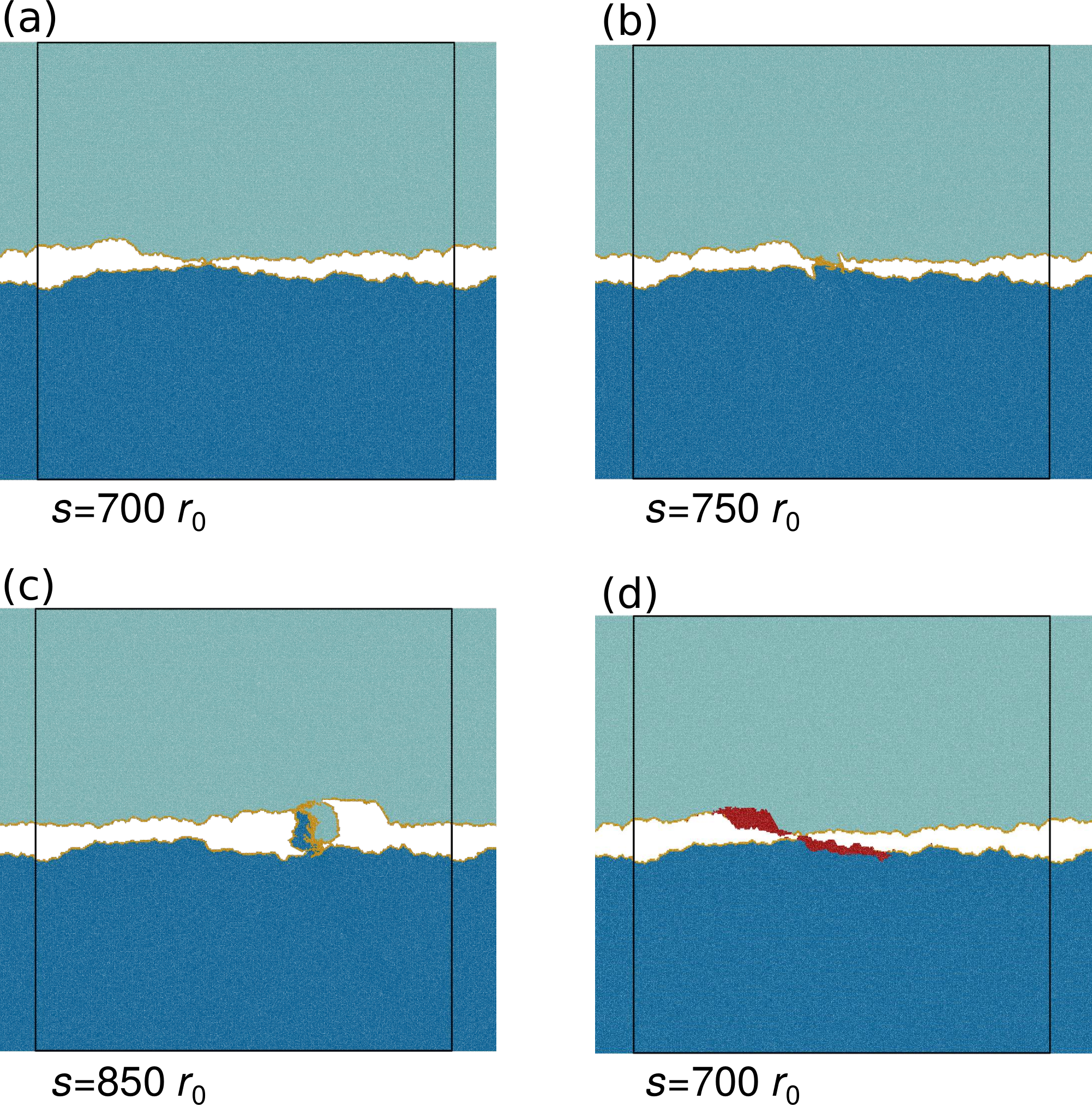
Within the 135 simulations, two different scenarios are observed. Scenario 1: the initial collisions lead to the formation of a distinct wear debris particle – this is observed in of the cases ( simulations). Scenario 2: multiple interacting contact junctions form or the contact spreads throughout the whole system, and a debris particle of characteristic size or larger would be formed. In such cases, cracks propagate from the surface until they reach the boundaries of the system (Figure 1(c)) or the surfaces weld at the interface (Figure 1(d)). In the latter case, the periodic boundary conditions suppress any stress concentration required for crack propagation, and a larger system size would be needed to observe cracks that lead to debris particle formation. Because in Scenario 2 cracks either reach the boundaries of the simulation cell (Figure 1(c)) or are inhibited (Figure 1(d)), simulations that display such scenario are discarded from the analysis. Scenario 2 is observed in the remaining ( simulations).
The likelihood of one scenario or the other correlates with the root mean square of heights of the initial surfaces (see Supplementary Table S.IV). This is due to the fact that, for a given value of , the rougher the surface, the more pronounced the asperities and valleys, and the system is more likely to form a junction size smaller than the system size (Scenario 1). When surfaces are smooth, the probability of having multiple contact spots that interact and/or coalesce is larger, and the system is more likely to attempt to create a particle of characteristic size or larger (i.e. Scenario 2).
Scenario 1 is also observed more often when adhesion is larger (see Supplementary Table S.IV). A reduction in is expected to reduce the junction shear strength and thus to increase the critical length scale (see Eq. 1). As the system needs a larger junction size to create a debris particle, contact can develop at other places at the same time, increasing the likelihood of Scenario 2.
Note that when the surface roughness and the interfacial adhesion are minimum, i.e. and , no simulation displayed Scenario 1, consistent with the two effects that were just described.
For the subset of simulations that exhibit Scenario 1, i.e. a debris particle smaller than the system size is formed, the initial volume is investigated. For this, an unambiguous definition of is needed, and we use the tangential force as a reference. When the two surfaces first come into contact, the tangential force starts increasing. After a peak is reached, the force decreases, signaling debris particle formation and the onset of rolling (Figure 2). We thus define as the volume of the debris particle measured at the first local minimum exhibited by , after the initial peak, as it corresponds to the work needed to form the debris particle Aghababaei et al. 2017. Identified volumes are then checked for erroneous measures, which are discarded. Erroneous measures are due to false positives of the particle detection algorithm and to the tangential force exhibiting a peak and a following local minimum when the particle is not formed yet (e.g. because of an initial ductile event). This procedure allows us to compare consistent values of from the different simulations.

The data for is reported in Figure 3 and Supplementary Tables S.I, S.II, S.III, and S.IV. We observe (Supplementary Table S.IV) that the average value of the initial volume increases with , contrary to Eq. 1. While at first this seems surprising, as lower values of imply larger , we argue that this is an artifact of the system size for low values of . When reducing , more simulations display in fact Scenario 2, i.e. the system attempts to form a debris particle that is too large with respect to the simulation cell. These cases are then not captured by the values of that we measured.
When identical initial geometries are compared (i.e. for the same values of ), no correlation between the strength of adhesion and the initial volume arises. This leads to the observation that the randomness of the initial surface morphology governs the debris particle formation, in contrast to what is observed at long timescales, where the effect of adhesion is significant (see Wear rate paragraph).
We now investigate the effects of the interfacial adhesion and the morphology on the minimum size of the generated debris particle. We know that the critical length scale governs the particle formation process, and that the strength of the interface enters the definition of by affecting : Once a junction of size is formed, if the interface is weak the asperities slide against one another, otherwise they deform plastically Brink and Molinari 2019. We thus rewrite Eq. 1 to make explicit the effect of the interfacial adhesion,
| (10) |
where at the denominator the junction shear strength in the case of reduced interfacial adhesion is expressed as a reduction of the junction shear strength of the full adhesion case (), with the proportionality given by for the potentials adopted in this work Aghababaei et al. 2016. In the limiting case of atomistically flat surfaces with semicircular asperities, this correctly predicts wear particle volumes that are larger when the interface is weaker Aghababaei 2019. To verify such prediction in the case of random rough surfaces, we assume that the minimum initial volume is given by a circular particle (in two dimensions), i.e.
| (11) |
is then minimum when is minimum and is maximum, and vice versa. In our work, the extreme values of are the minimum and maximum input values, i.e. and . The geometrical factor is instead determined by the geometry of contact, which is hard to obtain in our case of self-affine surfaces. The two limiting cases that we assume for our simulations are flat contact (, see Supplementary Methods) Pham-Ba et al. 2019 and contact between well-defined semicircular asperities () Aghababaei et al. 2016; Brink and Molinari 2019. If the reduced interfacial adhesion would play a key role in the initial debris particle volume , we would thus expect that
| (12) |
where is the initial volume observed in our simulations and which is reported in Figure 3. The green shaded area in Figure 3 depicts the values of , where the limiting cases of and are given by the lower green dotted line and the upper green dashed line, respectively. Our results show that the initial debris particle volume does not obey the trend of Eq. 12, as we observe volumes measured for that are smaller than the expected lower bound .
This shows that changes in the interfacial adhesion do not affect significantly the initial volume of the debris particle. Instead, we observe that all the recorded values of are larger than (solid purple line in Figure 3), determined from the minimum given in the full adhesion case ( , with the values of , , as in Ref. Aghababaei et al. 2016). We ascribe such behavior to the morphology of the surfaces, which in the current work is random. Recently, a refined version of Eq. 1 was derived Brink and Molinari 2019, where the junction shear strength depends on the angle of contact between the two ideal asperities. It was shown that if the angle of contact is larger than a critical value, the junction shear strength is given by and independent of . In the case of contact between self-affine surfaces, the contact junction is rough and the concept of angle of contact is ill-defined. Interlocking is thus expected in at least some cases. Furthermore, we argue that the ratio between the contact size and the thickness of the passivated layer also plays a significant role in the value of and, thus, of . In our simulations, the junction size is much larger than the passivated layer, which is thin when the surfaces come into contact. The bulk strength thus markedly affects the junction strength , which can be approximated by . If the thickness of the passivated layer were larger than the contact size, then we would expect to be influenced by and thus to be close to the reduced adhesion value . (Note that in such case a proportional reduction in the fracture energy is also expected, but the effect on is squared and thus .)
We also recall that for the smoothest cases ( ), the likelihood of Scenario 1 correlates with the strength of the interfacial adhesion (Supplementary Table S.IV). This is consistent with the aforementioned argument that when the contact interface is thin enough (compared with the passivated layer), affects the minimum debris particle volume (Eq. 10 and 11), as interlocking is less likely to occur.
We thus find that for the general case of rough surfaces, and for the conditions here investigated, the surface morphology dominates the minimum size of the wear debris particles. This appears independent of reductions in the interfacial adhesion strength (within the explored range of values of reduced adhesion), and is determined by the junction shear strength in the full adhesion case (i.e. by the bulk shear strength). We do not expect the surface morphology to necessarily dominate the average size of the wear particles, where effects of interfacial adhesion are expected to emerge – larger system sizes than those used in this set of simulations are needed to explore this question.
III.2 Long timescale self-affine morphology
Self-affine objects differ from self-similar ones by displaying anisotropic instead of isotropic scaling Barabási and Stanley 1995. For a one-dimensional surface, the scaling relation is expressed as Barabási and Stanley 1995; Meakin 1998, where is a function describing the surface heights as a function of the spatial coordinate , is the scaling factor, and is the Hurst (or roughness) exponent Meakin 1998; Mandelbrot 1985. This relation shows how the heights scale differently than the horizontal distances, with the scaling exponent. For physical surfaces, the Hurst exponent is constrained between and . In the limit isotropic scaling and, thus, self-similarity are recovered. The interest in the self-affine description of surfaces lies in the fact that, for such objects, the statistics of the surface are known at any scale once the Hurst exponent is also known. This allows to gather meaningful insights at the scale that is most convenient to investigate.
To investigate the effects of the reduced interfacial adhesion on the long term evolution of the surface morphology, the set of simulations L was prepared. It is characterized by long-timescale simulations – the shortest simulated sliding distance being and the longest . Within this set, simulations differ in the interfacial adhesion (), the initial Hurst exponent of the surfaces (), and the random seed used to generate the initial fractal surfaces. We selected such values of to avoid that the initial surfaces are already characterized by the same roughness observed at long timescales Milanese et al. 2019; Renard et al. 2013; Brodsky et al. 2016. The simulations of this group are identified by a code where the first letter is ’L’ for ’long timescale’, the following three digits represents the value of the interfacial adhesion , and the last letter identifies a set of values . The simulation L-100-B, for instance, indicates a long timescale simulation, with full adhesion at the interface, and . The length of the investigated timescales ensures that the whole running-in phase is over and a steady-state for the roughness in terms of equivalent root mean square of heights is reached, allowing to analyze the surface morphology in the steady-state Milanese et al. 2019. The initial geometry is then forgotten by the system and the measured morphology is a consequence of the frictional process. During each simulation, four stages are observed. Initially, the surfaces come into contact, possibly at multiple locations as the surfaces are randomly rough. The contacting spots then deform plastically, until the junction size is larger than and a debris particle is formed (Figures 4(a) and 4(c)). The wear particle is then constrained to roll between the surfaces, if the interfacial adhesion is large enough (Figure 4(b)). Otherwise, if the adhesion is low, the particle alternates between rolling and sticking to one surface (while sliding against the other one, Figures 4(d-f)). When the particle rolls between the two surfaces, these are continuously worn as material is transferred back and forth between the particle and each surface.

To determine if the resulting surfaces are self-affine, we investigate both their power spectral density per unit length and their height–height correlation function , where and are respectively the wavevector and the horizontal distance between two given points on the surface. It is known in fact that, for self-affine 1D profiles, they scale as Mandelbrot 1985; Ganti and Bhushan 1995; Berry and Lewis 1980 and Barabási and Stanley 1995, respectively (see Methods for more details).
Figure 5 and Supplementary Figure S.2 report the results of the surface analysis for the simulations in set L. The data are averaged over different independent surfaces extracted during the steady-state roughness (in terms of equivalent root mean square of heights ) that follows the running-in phase Milanese et al. 2019; Kragelsky et al. 1981; Rabinowicz 1995. While it is known that in the full adhesion case () surfaces display a self-affine morphology characterized by a persistent Hurst exponent Milanese et al. 2019, it is observed here that the self-affine description holds also in the case of reduced interfacial adhesion (), but under some conditions.
We thus investigated the distance travelled by the debris particle in each simulation (see Figure 4 and Supplementary Figure S.4). We observe that, in simulations for which or , the particle travelled a comparable distance (between and ) among the different simulations, and in all cases the surfaces exhibit self-affine behavior (see Figure 5 and Supplementary Figure S.2). The travelled distance is consistent with the estimation of that is expected for a particle in perfect rolling conditions. To explain this expected value of , let us assume that both the particle and the surfaces are rigid, with the top surface sliding at constant velocity and the bottom one fixed. The highest point of the particle is then in contact with the top surface and must be sliding at velocity . Similarly, the lowest point is in contact with the bottom surface and its velocity is zero. The center of the particle (which coincides with the center of mass) then rolls at velocity , and the travelled distance is half the one of the top surface, within a given time period. When , the travelled distance is markedly different, the value at the end of the simulations being between and (see Figure 4 and Supplementary Figure S.4) or over (see Supplementary Figure S.4). These Figures show that the particle undergoes long periods where it continuously slides against one of the surfaces (sticking to the other one), as significant portions at constant slope (sticking to bottom fixed surface) and (sticking to top sliding surface) confirm. During these periods, the particle does not roll and only works the surface against which it slides, with mechanisms that differ from the ones that take place during rolling. This is reflected by larger values of (see Figure 6) and the surfaces not always being characterized by a self-affine morphology (see Figure 5). We believe that longer sliding distances would compensate for this effect, i.e. the travelled distance and the rolled distance would increase, allowing for the working of the surfaces that leads to the fractal morphology observed for larger values of the interfacial adhesion. This observation strengthens the hypothesis Milanese et al. 2019 that a frictional system needs to develop third bodies that work the surfaces for them to evolve into a self-affine topography.
III.3 Wear rate
The length of simulations in set L allows us to investigate also the wear rate over long distances for different values of the interfacial adhesion. Figures 6(b) and Supplementary Figure S.3(b) show the evolution of the wear volume with the sliding distance . Simulations with the lowest interfacial adhesion () display a markedly different behavior than the persistent increase in volume commonly expected, and observed for the full adhesion case Milanese et al. 2019. For reduced interfacial adhesion cases, the wear volume is characterized mostly by an almost zero wear rate, the particle volume being determined upon formation. This is due to the long sticking time. The low interfacial adhesion reduces or inhibits material transfer between the particle and the surface it slides against. And evidently no material is transferred between the particle and the surface it sticks to. Therefore the sliding motion involves only mutual deformation of the two bodies, without significant transfer of atoms (if anything, the wear particle seems to lose mass in some cases). After long periods of sticking, the deformation that takes place in the two bodies is such that the debris particle is again detached from surface it sticks to. For example, during such a period of sticking, the particle can be pushed into a valley, then forced out of it by a fracture-like event and finally it rolls for a while, until it sticks again (Figure 4(c-f)). These rare events can lead to significant local increases in the particle volume, as the detachment is fracture induced in a two-body configuration (Figure 6 and Supplementary Figure S.3). The growth of the debris particle volume in the low interfacial adhesion case is then not continuous and is controlled by rare fracture events.
The case for falls between the full and low adhesion cases. While the debris particle does not display extended sticking times, the growth rate is significantly lower than in full adhesion conditions. Rare fracture events can happen and significantly affect the wear debris volume, but they are not the predominant mechanism for mass transfer between the surfaces and the debris particle.
IV Discussion
In this study, we performed 2D molecular dynamics simulations of frictional systems to investigate the effect of reductions in the interfacial adhesion strength and initial surface morphology on three aspects of the adhesive wear process: the minimum size of loose wear particles, the long-term evolution of the surface roughness, and the wear rate. Our results show that, within the high adhesion regime that we explored, reducing the interfacial adhesion does not fundamentally change the nature of the processes occurring when two rough surfaces slide against one another and transition into a three-body configuration.
When the initial surfaces are self-affine, as is commonly expected in real applications, reducing the interfacial adhesion does not significantly affect the minimum initial volume of the debris particle that forms in the early stages of the sliding process. The random surface morphology thus governs the minimum size of the debris particles, which is then predicted by the critical length scale estimated with the values of the bulk properties (full adhesion situation). This is potentially relevant to the many engineering applications where the minimum size of wear fragments is of particular interest – for instance in the transport industry, where particle emissions play an important role in health hazards that are linked to airborne particles.
Reduced interfacial adhesion nevertheless slows down some of the processes taking place during adhesive wear, namely the evolution of the surfaces into a self-affine morphology and the debris particle growth. Over long timescales, low values of interfacial adhesion increase the possibility of the debris particle to continuously slide against one of the surfaces (and stick to the other one), almost in a temporary two-body configuration, altering the wear mechanisms. If such periods are not too long with respect to the sliding distance, the particle still has time to roll against the surfaces and work them, and the surfaces finally exhibit a self-affine morphology, otherwise no fractal scaling is observed. Furthermore, during these periods where the particle sticks to one surface, the wear rate decreases significantly and it can become negligible.
Finally, we note that these conclusions are drawn on the basis of two-dimensional simulations, as the investigated long timescales are computationally challenging for three-dimensional systems. While analogous observations have been previously extended from 2D to 3D Aghababaei et al. 2016; Aghababaei et al. 2017; Brink and Molinari 2019, further work is needed to extend our conclusions to three-dimensional systems and to engineering applications.
References
- Samet et al. (2000) J. M. Samet, F. Dominici, F. C. Curriero, I. Coursac, and S. L. Zeger, Fine particulate air pollution and mortality in 20 us cities, 1987–1994, New England Journal of Medicine 343, 1742 (2000).
- Pope III et al. (2002) C. A. Pope III, R. T. Burnett, M. J. Thun, E. E. Calle, D. Krewski, K. Ito, and G. D. Thurston, Lung cancer, cardiopulmonary mortality, and long-term exposure to fine particulate air pollution, Jama 287, 1132 (2002).
- Olofsson (2011) U. Olofsson, A study of airborne wear particles generated from the train traffic—block braking simulation in a pin-on-disc machine, Wear 271, 86 (2011).
- Rabinowicz (1995) E. Rabinowicz, Friction and wear of materials (Wiley, New York, 1995).
- Godet (1984) M. Godet, The third-body approach: a mechanical view of wear, Wear 100, 437 (1984).
- Bhaskaran et al. (2010) H. Bhaskaran, B. Gotsmann, A. Sebastian, U. Drechsler, M. A. Lantz, M. Despont, P. Jaroenapibal, R. W. Carpick, Y. Chen, and K. Sridharan, Ultralow nanoscale wear through atom-by-atom attrition in silicon-containing diamond-like carbon, Nature Nanotechnology 5, 181 (2010).
- Schirmeisen (2013) A. Schirmeisen, Wear: One atom after the other, Nature nanotechnology 8, 81 (2013).
- Jacobs and Carpick (2013) T. D. Jacobs and R. W. Carpick, Nanoscale wear as a stress-assisted chemical reaction, Nature Nanotechnology 8, 108 (2013).
- Yang et al. (2016) Y. Yang, L. Huang, and Y. Shi, Adhesion suppresses atomic wear in single-asperity sliding, Wear 352, 31 (2016).
- Shao et al. (2017) Y. Shao, T. D. Jacobs, Y. Jiang, K. T. Turner, R. W. Carpick, and M. L. Falk, Multibond model of single-asperity tribochemical wear at the nanoscale, ACS Applied Materials & Interfaces 9, 35333 (2017).
- Liu et al. (2017) J. Liu, Y. Jiang, D. S. Grierson, K. Sridharan, Y. Shao, T. D. Jacobs, M. L. Falk, R. W. Carpick, and K. T. Turner, Tribochemical wear of diamond-like carbon-coated atomic force microscope tips, ACS Applied Materials & Interfaces 9, 35341 (2017).
- Aghababaei et al. (2016) R. Aghababaei, D. H. Warner, and J.-F. Molinari, Critical length scale controls adhesive wear mechanisms, Nature Communications 7 (2016).
- Holm (1946) R. Holm, Electric contacts (Almqvist and Wiksells, Stockholm, 1946).
- Merkle and Marks (2008) A. P. Merkle and L. D. Marks, Liquid-like tribology of gold studied by in situ tem, Wear 265, 1864 (2008).
- Milanese et al. (2019) E. Milanese, T. Brink, R. Aghababaei, and J.-F. Molinari, Emergence of self-affine surfaces during adhesive wear, Nature Communications 10, 1116 (2019).
- Archard (1953) J. Archard, Contact and rubbing of flat surfaces, Journal of Applied Physics 24, 981 (1953).
- Liu et al. (2010a) J. Liu, J. K. Notbohm, R. W. Carpick, and K. T. Turner, Method for characterizing nanoscale wear of atomic force microscope tips, ACS Nano 4, 3763 (2010a).
- Liu et al. (2010b) J. Liu, D. S. Grierson, N. Moldovan, J. Notbohm, S. Li, P. Jaroenapibal, S. O’Connor, A. Sumant, N. Neelakantan, J. A. Carlisle, et al., Preventing nanoscale wear of atomic force microscopy tips through the use of monolithic ultrananocrystalline diamond probes, Small 6, 1140 (2010b).
- Aghababaei et al. (2017) R. Aghababaei, D. H. Warner, and J.-F. Molinari, On the debris-level origins of adhesive wear, Proceedings of the National Academy of Sciences 114, 7935 (2017).
- Aghababaei et al. (2018) R. Aghababaei, T. Brink, and J.-F. Molinari, Asperity-level origins of transition from mild to severe wear, Physical Review Letters 120, 186105 (2018).
- Frérot et al. (2018) L. Frérot, R. Aghababaei, and J.-F. Molinari, A mechanistic understanding of the wear coefficient: From single to multiple asperities contact, Journal of the Mechanics and Physics of Solids 114, 172 (2018).
- Pham-Ba et al. (2019) S. Pham-Ba, T. Brink, and J.-F. Molinari, Adhesive wear and interaction of tangentially loaded micro-contacts, International Journal of Solids and Structures (2019).
- Brink and Molinari (2019) T. Brink and J.-F. Molinari, Adhesive wear mechanisms in the presence of weak interfaces: Insights from an amorphous model system, Physical Review Materials 3, 053604 (2019).
- Aghababaei (2019) R. Aghababaei, Effect of adhesion on material removal during adhesive wear, Physical Review Materials 3, 063604 (2019).
- Renard et al. (2013) F. Renard, T. Candela, and E. Bouchaud, Constant dimensionality of fault roughness from the scale of micro-fractures to the scale of continents, Geophysical Research Letters 40, 83 (2013).
- Sayles and Thomas (1978) R. S. Sayles and T. R. Thomas, Surface topography as a nonstationary random process, Nature 271, 431 (1978).
- Majumdar and Tien (1990) A. Majumdar and C. Tien, Fractal characterization and simulation of rough surfaces, Wear 136, 313 (1990).
- Persson et al. (2004) B. Persson, O. Albohr, U. Tartaglino, A. Volokitin, and E. Tosatti, On the nature of surface roughness with application to contact mechanics, sealing, rubber friction and adhesion, Journal of Physics: Condensed Matter 17, R1 (2004).
- Morse (1929) P. M. Morse, Diatomic molecules according to the wave mechanics. II. Vibrational levels, Physical Review 34, 57 (1929).
- Plimpton (1995) S. Plimpton, Fast parallel algorithms for short-range molecular dynamics, Journal of Computational Physics 117, 1 (1995).
- Jacobs et al. (2017) T. D. Jacobs, T. Junge, and L. Pastewka, Quantitative characterization of surface topography using spectral analysis, Surface Topography: Metrology and Properties 5, 013001 (2017).
- Barabási and Stanley (1995) A.-L. Barabási and H. E. Stanley, Fractal concepts in surface growth (Cambridge university press, 1995).
- Meakin (1998) P. Meakin, Fractals, scaling and growth far from equilibrium, Vol. 5 (Cambridge university press, 1998).
- Mandelbrot (1985) B. B. Mandelbrot, Self-affine fractals and fractal dimension, Physica Scripta 32, 257 (1985).
- Ganti and Bhushan (1995) S. Ganti and B. Bhushan, Generalized fractal analysis and its applications to engineering surfaces, Wear 180, 17 (1995).
- Berry and Lewis (1980) M. Berry and Z. Lewis, On the Weierstrass-Mandelbrot fractal function, in Proceedings of the Royal Society of London A: Mathematical, Physical and Engineering Sciences, Vol. 370 (The Royal Society, 1980) pp. 459–484.
- Press et al. (2007) W. H. Press, S. A. Teukolsky, W. T. Vetterling, and B. P. Flannery, Numerical recipes 3rd edition: The art of scientific computing (Cambridge university press, 2007).
- VanderPlas (2018) J. T. VanderPlas, Understanding the Lomb–Scargle periodogram, The Astrophysical Journal Supplement Series 236, 16 (2018).
- Bhushan (2000) B. Bhushan, Surface roughness analysis and measurement techniques, in Modern tribology handbook, two volume set, edited by B. Bhushan (CRC press, 2000) Chap. 4, pp. 49–120.
- Stukowski (2009) A. Stukowski, Visualization and analysis of atomistic simulation data with OVITO–the Open Visualization Tool, Modelling and Simulation in Materials Science and Engineering 18, 015012 (2009).
- Kirkpatrick et al. (1983) S. Kirkpatrick, C. D. Gelatt, and M. P. Vecchi, Optimization by simulated annealing, Science 220, 671 (1983).
- Metropolis et al. (1953) N. Metropolis, A. W. Rosenbluth, M. N. Rosenbluth, A. H. Teller, and E. Teller, Equation of state calculations by fast computing machines, The Journal of Chemical Physics 21, 1087 (1953).
- Brodsky et al. (2016) E. E. Brodsky, J. D. Kirkpatrick, and T. Candela, Constraints from fault roughness on the scale-dependent strength of rocks, Geology 44, 19 (2016).
- Kragelsky et al. (1981) I. V. Kragelsky, M. N. Dobychin, and V. S. Kombalov, Friction and wear: calculation methods (Pergamon Press, 1981).
Supplemental Material
See Supplemental Material at (URL by publisher) for supplementary methods, figures, and tables referenced in the main text.
Acknowledgements
This work was supported by EPFL through the use of the facilities of its Scientific IT and Application Support Center.
Authors Contributions
E. M. performed the numerical simulations and the analyses. R. A. developed the algorithm to detect surface atoms and re-assign the interfacial adhesion potential on-the-fly. E. M., T. B., and J.-F. M. planned the simulations sets and the wrote the manuscript. All authors participated in the discussion.
Supplementary Materials
IV.1 Supplementary methods
Geometrical factor for flat contacts
In the original formulation of Ref. Aghababaei et al. 2016, the critical length scale for the ductile-to-brittle transition stems from a Griffith-like criterion applied to asperities of a generic shape. According to the criterion, if the elastic energy is larger or equal than the adhesive energy , crack propagation is favoured over plastic deformation, and a debris particle is formed. As the two energies scale as and , the minimum contact junction size at which crack propagation takes place is found for and it has the form
| (13) |
where is the junction shear strength (and in the general case depends on ), is the shear modulus of the material, is twice the fracture energy and is a geometrical factor. In the derivation of Eq. 13, it is assumed that the elastic energy is fully contained in the asperity volume, which is uniformly loaded at the shear junction strength . thus depends on both the characteristic size and the shape of the asperity. also depends on both, as the shape of the asperity defines the crack path and, consequently, the free surfaces that needs to be created in the fracture process. The geometrical factor takes into account the shape of the asperities and the actual stress distribution (due to this shape). The meaning of is clear in the expression of if Eq. 13 is rewritten in the form used in the main text (Eq. 1)
| (14) |
where regulates the ratio between the fracture energy and the stored elastic energy density . In Ref. Aghababaei et al. 2016, data from molecular dynamics simulations shows that for well-defined semicircular asperities in 2D.
More recently, another formulation for in two dimensions was derived based on an analytical approach in Ref. Pham-Ba et al. 2019. Here, the asperity is replaced by a distributed constant shear load of magnitude applied along a length on the flat surface of a semi-infinite body. An analytical expression for in the whole body is then provided. The value of then depends on the length of contact (i.e. the characteristic size of the debris particle to be detached), but not on the shape of the debris particle that is detached. The expression of the elastic energy is then
| (15) |
where for plane stress and for plane strain ( and being the elastic modulus and the Poisson ratio of the material), is the thickness of the semi-infinite body along the direction, and is an infinite integral term in 2D,
| (16) |
The shape of the detached particle still defines the crack path, and in Ref. Pham-Ba et al. 2019 it assumed to be semi-circular. This leads to the adhesive energy
| (17) |
where is the surface energy of the material, and two semi-circular surfaces of circumference are created. The critical length scale is found again by imposing the condition , and it is (for plane stress, as in our simulations)
| (18) |
As and, for the model potentials adopted in Ref. Aghababaei et al. 2016 and in this work, , we can express in terms of :
| (19) |
The integral is finite in our case, as it is bounded by the plastic zone ( ), where the integral is capped () and the height of the body along the direction ( ). It is then , and
| (20) |
which is true if . In the flat contact case, is then smaller than the empirical value of found in Ref. Aghababaei et al. 2016 for the asperity case.
In the simulations of this current work, the first contact takes place between two rough self-affine surfaces, for which the concept of asperity is ill-defined. Furthermore, when the root mean square of heights of the surfaces is small, the collision between the two bodies is close to the flat contact situation. This is shown in Supplementary Figure S.5, where it is also observed that the areas that contribute to the detached particle are not semicircular (red atoms in Supplementary Figure S.5(d)). We thus derive for the general case of a semi-elliptical detached particle. Note that, as previously explained, the elastic energy contained in the body is independent of the shape of the detached particle, and we need to generalize only the expression for .
As no exact formula for the perimeter of an ellipse exists, we rely on the second Ramanujan approximation, which provides an accurate estimation also in the limiting case (two overlapping segments), and being the axes of the ellipse. The formula gives the perimeter as
| (21) |
where
| (22) |
We substitute for and , where we assume that the major axis is the contact junction and that the proportionality of the minor axis to the major axis is given by the scalar . Expressions 21 and 22 become
| (23) | |||
| (24) |
where
| (25) |
The adhesive energy (Eq. 17) is now expressed as
| (26) |
and the critical length scale (Eq. 18) becomes
| (27) |
The two limit cases are (circular particle), for which and Equations 18 and 20 are recovered, and (two overlapping segments), for which , and is
| (28) |
and .
Supplementary Figure S.5(e) shows the variation of as a function of the factor , and it grows sub-linearly for small values of , i.e. a high eccentricity of the ellipse gives values of close to .
In the case of the simulations of Supplementary Figure S.5(a-d), we can derive the minor and major axes and from the position at the first contact of the atoms that will later form the debris particle (Supplementary Figure S.5(d)). The atoms describe two distinct portions, one on each surfaces, whose maximum and minimum lengths are estimated. The average of the two minimum (maximum) lengths gives us an approximation of the axis (), and, thus, . We can then compute from Eq. 27, which gives .
IV.2 Supplementary figures

IV.3 Supplementary Tables
| ID | seed | scenario | ||||
| S-100-01 | 1.00 | 0.5 | 5 | 19 | 1 | 6.50 |
| S-100-02 | 1.00 | 0.5 | 5 | 32 | 1 | 7.34 |
| S-100-03 | 1.00 | 0.5 | 5 | 42 | 1 | 0.97 |
| S-100-04 | 1.00 | 0.5 | 5 | 66 | 2 | n/a |
| S-100-05 | 1.00 | 0.5 | 5 | 91 | 1 | disc. |
| S-100-06 | 1.00 | 0.7 | 5 | 19 | 1 | 9.32 |
| S-100-07 | 1.00 | 0.7 | 5 | 32 | 1 | 11.19 |
| S-100-08 | 1.00 | 0.7 | 5 | 42 | 2 | n/a |
| S-100-09 | 1.00 | 0.7 | 5 | 66 | 2 | n/a |
| S-100-10 | 1.00 | 0.7 | 5 | 91 | 2 | n/a |
| S-100-11 | 1.00 | 1.0 | 5 | 19 | 1 | 8.53 |
| S-100-12 | 1.00 | 1.0 | 5 | 32 | 1 | 8.55 |
| S-100-13 | 1.00 | 1.0 | 5 | 42 | 2 | n/a |
| S-100-14 | 1.00 | 1.0 | 5 | 66 | 1 | 40.34 |
| S-100-15 | 1.00 | 1.0 | 5 | 91 | 2 | n/a |
| S-100-16 | 1.00 | 0.5 | 10 | 19 | 2 | n/a |
| S-100-17 | 1.00 | 0.5 | 10 | 32 | 2 | n/a |
| S-100-18 | 1.00 | 0.5 | 10 | 42 | 2 | n/a |
| S-100-19 | 1.00 | 0.5 | 10 | 66 | 1 | disc. |
| S-100-20 | 1.00 | 0.5 | 10 | 91 | 1 | 11.68 |
| S-100-21 | 1.00 | 0.7 | 10 | 19 | 1 | disc. |
| S-100-22 | 1.00 | 0.7 | 10 | 32 | 1 | disc. |
| S-100-23 | 1.00 | 0.7 | 10 | 42 | 2 | n/a |
| S-100-24 | 1.00 | 0.7 | 10 | 66 | 1 | disc. |
| S-100-25 | 1.00 | 0.7 | 10 | 91 | 1 | 10.39 |
| S-100-26 | 1.00 | 1.0 | 10 | 19 | 2 | n/a |
| S-100-27 | 1.00 | 1.0 | 10 | 32 | 2 | n/a |
| S-100-28 | 1.00 | 1.0 | 10 | 42 | 2 | n/a |
| S-100-29 | 1.00 | 1.0 | 10 | 66 | 1 | disc. |
| S-100-30 | 1.00 | 1.0 | 10 | 91 | 1 | 11.24 |
| S-100-31 | 1.00 | 0.5 | 20 | 19 | 1 | 11.13 |
| S-100-32 | 1.00 | 0.5 | 20 | 32 | 1 | disc. |
| S-100-33 | 1.00 | 0.5 | 20 | 42 | 2 | n/a |
| S-100-34 | 1.00 | 0.5 | 20 | 66 | 1 | 11.08 |
| S-100-35 | 1.00 | 0.5 | 20 | 91 | 1 | 2.20 |
| S-100-36 | 1.00 | 0.7 | 20 | 19 | 1 | 20.25 |
| S-100-37 | 1.00 | 0.7 | 20 | 32 | 1 | 18.49 |
| S-100-38 | 1.00 | 0.7 | 20 | 42 | 1 | 7.82 |
| S-100-39 | 1.00 | 0.7 | 20 | 66 | 1 | disc. |
| S-100-40 | 1.00 | 0.7 | 20 | 91 | 1 | disc. |
| S-100-41 | 1.00 | 1.0 | 20 | 19 | 1 | 15.28 |
| S-100-42 | 1.00 | 1.0 | 20 | 32 | 1 | 12.50 |
| S-100-43 | 1.00 | 1.0 | 20 | 42 | 1 | 2.83 |
| S-100-44 | 1.00 | 1.0 | 20 | 66 | 1 | 9.74 |
| S-100-45 | 1.00 | 1.0 | 20 | 91 | 1 | disc. |
| ID | seed | scenario | ||||
| S-080-01 | 0.80 | 0.5 | 5 | 19 | 2 | n/a |
| S-080-02 | 0.80 | 0.5 | 5 | 32 | 1 | disc. |
| S-080-03 | 0.80 | 0.5 | 5 | 42 | 2 | n/a |
| S-080-04 | 0.80 | 0.5 | 5 | 66 | 2 | n/a |
| S-080-05 | 0.80 | 0.5 | 5 | 91 | 2 | n/a |
| S-080-06 | 0.80 | 0.7 | 5 | 19 | 2 | n/a |
| S-080-07 | 0.80 | 0.7 | 5 | 32 | 1 | 6.63 |
| S-080-08 | 0.80 | 0.7 | 5 | 42 | 2 | n/a |
| S-080-09 | 0.80 | 0.7 | 5 | 66 | 2 | n/a |
| S-080-10 | 0.80 | 0.7 | 5 | 91 | 2 | n/a |
| S-080-11 | 0.80 | 1.0 | 5 | 19 | 1 | disc. |
| S-080-12 | 0.80 | 1.0 | 5 | 32 | 2 | n/a |
| S-080-13 | 0.80 | 1.0 | 5 | 42 | 2 | n/a |
| S-080-14 | 0.80 | 1.0 | 5 | 66 | 2 | n/a |
| S-080-15 | 0.80 | 1.0 | 5 | 91 | 2 | n/a |
| S-080-16 | 0.80 | 0.5 | 10 | 19 | 2 | n/a |
| S-080-17 | 0.80 | 0.5 | 10 | 32 | 2 | n/a |
| S-080-18 | 0.80 | 0.5 | 10 | 42 | 2 | n/a |
| S-080-19 | 0.80 | 0.5 | 10 | 66 | 2 | n/a |
| S-080-20 | 0.80 | 0.5 | 10 | 91 | 1 | disc. |
| S-080-21 | 0.80 | 0.7 | 10 | 19 | 2 | n/a |
| S-080-22 | 0.80 | 0.7 | 10 | 32 | 1 | disc. |
| S-080-23 | 0.80 | 0.7 | 10 | 42 | 2 | n/a |
| S-080-24 | 0.80 | 0.7 | 10 | 66 | 1 | 2.61 |
| S-080-25 | 0.80 | 0.7 | 10 | 91 | 1 | 12.09 |
| S-080-26 | 0.80 | 1.0 | 10 | 19 | 1 | disc. |
| S-080-27 | 0.80 | 1.0 | 10 | 32 | 2 | n/a |
| S-080-28 | 0.80 | 1.0 | 10 | 42 | 2 | n/a |
| S-080-29 | 0.80 | 1.0 | 10 | 66 | 2 | n/a |
| S-080-30 | 0.80 | 1.0 | 10 | 91 | 1 | 8.28 |
| S-080-31 | 0.80 | 0.5 | 20 | 19 | 1 | disc. |
| S-080-32 | 0.80 | 0.5 | 20 | 32 | 1 | 7.08 |
| S-080-33 | 0.80 | 0.5 | 20 | 42 | 1 | disc. |
| S-080-34 | 0.80 | 0.5 | 20 | 66 | 1 | 4.97 |
| S-080-35 | 0.80 | 0.5 | 20 | 91 | 1 | 3.13 |
| S-080-36 | 0.80 | 0.7 | 20 | 19 | 1 | 13.70 |
| S-080-37 | 0.80 | 0.7 | 20 | 32 | 1 | 15.90 |
| S-080-38 | 0.80 | 0.7 | 20 | 42 | 1 | 0.34 |
| S-080-39 | 0.80 | 0.7 | 20 | 66 | 1 | 11.53 |
| S-080-40 | 0.80 | 0.7 | 20 | 91 | 1 | disc. |
| S-080-41 | 0.80 | 1.0 | 20 | 19 | 1 | 13.53 |
| S-080-42 | 0.80 | 1.0 | 20 | 32 | 1 | 15.65 |
| S-080-43 | 0.80 | 1.0 | 20 | 42 | 1 | 4.25 |
| S-080-44 | 0.80 | 1.0 | 20 | 66 | 1 | 12.04 |
| S-080-45 | 0.80 | 1.0 | 20 | 91 | 1 | 20.05 |
| ID | seed | scenario | ||||
| S-060-01 | 0.60 | 0.5 | 5 | 19 | 2 | n/a |
| S-060-02 | 0.60 | 0.5 | 5 | 32 | 2 | n/a |
| S-060-03 | 0.60 | 0.5 | 5 | 42 | 2 | n/a |
| S-060-04 | 0.60 | 0.5 | 5 | 66 | 2 | n/a |
| S-060-05 | 0.60 | 0.5 | 5 | 91 | 2 | n/a |
| S-060-06 | 0.60 | 0.7 | 5 | 19 | 2 | n/a |
| S-060-07 | 0.60 | 0.7 | 5 | 32 | 2 | n/a |
| S-060-08 | 0.60 | 0.7 | 5 | 42 | 2 | n/a |
| S-060-09 | 0.60 | 0.7 | 5 | 66 | 2 | n/a |
| S-060-10 | 0.60 | 0.7 | 5 | 91 | 2 | n/a |
| S-060-11 | 0.60 | 1.0 | 5 | 19 | 2 | n/a |
| S-060-12 | 0.60 | 1.0 | 5 | 32 | 2 | n/a |
| S-060-13 | 0.60 | 1.0 | 5 | 42 | 2 | n/a |
| S-060-14 | 0.60 | 1.0 | 5 | 66 | 2 | n/a |
| S-060-15 | 0.60 | 1.0 | 5 | 91 | 2 | n/a |
| S-060-16 | 0.60 | 0.5 | 10 | 19 | 2 | n/a |
| S-060-17 | 0.60 | 0.5 | 10 | 32 | 2 | n/a |
| S-060-18 | 0.60 | 0.5 | 10 | 42 | 2 | n/a |
| S-060-19 | 0.60 | 0.5 | 10 | 66 | 2 | n/a |
| S-060-20 | 0.60 | 0.5 | 10 | 91 | 1 | 5.47 |
| S-060-21 | 0.60 | 0.7 | 10 | 19 | 1 | 7.81 |
| S-060-22 | 0.60 | 0.7 | 10 | 32 | 2 | n/a |
| S-060-23 | 0.60 | 0.7 | 10 | 42 | 2 | n/a |
| S-060-24 | 0.60 | 0.7 | 10 | 66 | 2 | n/a |
| S-060-25 | 0.60 | 0.7 | 10 | 91 | 1 | 7.18 |
| S-060-26 | 0.60 | 1.0 | 10 | 19 | 1 | disc. |
| S-060-27 | 0.60 | 1.0 | 10 | 32 | 2 | n/a |
| S-060-28 | 0.60 | 1.0 | 10 | 42 | 2 | n/a |
| S-060-29 | 0.60 | 1.0 | 10 | 66 | 2 | n/a |
| S-060-30 | 0.60 | 1.0 | 10 | 91 | 1 | 4.08 |
| S-060-31 | 0.60 | 0.5 | 20 | 19 | 1 | 10.45 |
| S-060-32 | 0.60 | 0.5 | 20 | 32 | 1 | 10.42 |
| S-060-33 | 0.60 | 0.5 | 20 | 42 | 1 | 2.14 |
| S-060-34 | 0.60 | 0.5 | 20 | 66 | 1 | disc. |
| S-060-35 | 0.60 | 0.5 | 20 | 91 | 1 | 0.85 |
| S-060-36 | 0.60 | 0.7 | 20 | 19 | 1 | disc. |
| S-060-37 | 0.60 | 0.7 | 20 | 32 | 1 | 13.05 |
| S-060-38 | 0.60 | 0.7 | 20 | 42 | 1 | 2.04 |
| S-060-39 | 0.60 | 0.7 | 20 | 66 | 1 | 3.01 |
| S-060-40 | 0.60 | 0.7 | 20 | 91 | 1 | disc. |
| S-060-41 | 0.60 | 1.0 | 20 | 19 | 1 | disc. |
| S-060-42 | 0.60 | 1.0 | 20 | 32 | 1 | 13.02 |
| S-060-43 | 0.60 | 1.0 | 20 | 42 | 1 | disc. |
| S-060-44 | 0.60 | 1.0 | 20 | 66 | 1 | disc. |
| S-060-45 | 0.60 | 1.0 | 20 | 91 | 1 | 17.67 |
| Scenario 1 | Scenario 1 | Scenario 1 | Scenario 1 Total | ||
| 13.1 | |||||
| 11.0 | |||||
| 8.6 | |||||
| all | 10.9 |
| ID | seed | |||
| L-100-A | 1.0 | 0.3 | 29 | 339.314 |
| L-100-B | 1.0 | 0.3 | 42 | 339.314 |
| L-100-C | 1.0 | 1.0 | 29 | 339.314 |
| L-100-D | 1.0 | 1.0 | 42 | 339.314 |
| L-080-A | 0.8 | 0.3 | 29 | 339.314 |
| L-080-B | 0.8 | 0.3 | 42 | 339.314 |
| L-080-C | 0.8 | 1.0 | 29 | 339.314 |
| L-080-D | 0.8 | 1.0 | 42 | 339.314 |
| L-060-A | 0.6 | 0.3 | 29 | 339.314 |
| L-060-B | 0.6 | 0.3 | 42 | 339.314 |
| L-060-C | 0.6 | 1.0 | 29 | 339.314 |
| L-060-D | 0.6 | 1.0 | 42 | 339.314 |
| L-100-X | 1.0 | 0.3 | 42 | 678.627 |
| L-080-X | 0.8 | 0.3 | 42 | 678.627 |