Computation of Extremum Singular Values and
the Strong H-infinity Norm of SISO Time-Delay Systems

The availability of robust methods to compute $\mathcal{H}_{\infty}$ norms is essential in a computer aided control system design [15]. The common approaches for computing $\mathcal{H}_{\infty}$ norms for finite-dimensional linear systems, which belong to the class of level set methods, are based on the relation between the intersections of singular value curves of the transfer function with a constant function (the level) and the presence of imaginary axis eigenvalues of a corresponding Hamiltonian matrix [6]. In [6, 2] linearly converging bisection based algorithms have been proposed. Quadratically convergent algorithms, relying on an alternating search in two directions, have been described in [1, 5]. In [12] a level set algorithm for computing $\mathcal{H}_{\infty}$ norms of a class of retarded type time-delay systems has been outlined. The main complication with respect to the delay-free case is that the intersections between the singular value curves and a level set are no longer related to the spectrum of a Hamiltonian matrix, but to an infinite-dimensional operator. Therefore, the algorithm of [12] adopts a predictor-corrector approach, where in the first step the operator is discretized using a spectral method, followed by local corrections to remove the effect of the discretization on computed peak values in the frequency response. For the sake of completeness, it should be mentioned that for systems without delay, $\mathcal{H}_{\infty}$ norms can also be computed by a parameter sweep, thereby checking the feasibility of linear matrix inequalities, see, e.g., [13]. However, since these methods implicitly construct a Lyapunov function, and in the infinite-dimensional, time-delay case, fixing the form of the Lyapunov functional to a tractable form involving finitely many free parameters typically introduces conservatism, only potentially conservative bounds on the $\mathcal{H}_{\infty}$ norm can be aimed at in the latter case.

Inherent to level set methods, whether for systems with or without delay, is that the $\mathcal{H}_{\infty}$ norm is computed in an iterative way, by updating the level in every iteration step until convergence to the dominant peak in the singular value plot is achieved. In every iteration step the imaginary axis eigenvalues of a Hamiltonian matrix or operator need to be computed. As a first main contribution of the paper, we present a novel numerical algorithm to compute $\mathcal{H}_{\infty}$ norms of SISO time-delay systems requiring solving only one eigenvalue problem.

The second main contribution is that our method admits a system description in a standard form, described by a set of delay differential algebraic equations (DDAEs). As we will see, this form contains a large set of systems, including interconnections of time-delay systems and controllers in complex configurations, and including both retarded and neutral type systems.

Recently, we analyzed in [9] the properties of the $\mathcal{H}_{\infty}$ norm of time-delay systems. We illustrated that the $\mathcal{H}_{\infty}$ norm of DDAEs may be sensitive with respect to arbitrarily small delay perturbations. Due to this sensitivity, we introduced the strong $\mathcal{H}_{\infty}$ norm, which explicitly takes into account small delay perturbations, inevitable in any practical control application, and we outlined the computation using a level set approach. The derived theory of strong $\mathcal{H}_{\infty}$ norms can be considered as the dual of the theory of strong stability for neutral systems and DDAEs, as, e.g., elaborated in [10, 11] and the references therein. As a third, main contribution, the presented algorithm in this paper takes the potential sensitivity problem into account, by computing the strong $\mathcal{H}_{\infty}$ norm. In control problems without feed through at infinity along the loops, this strong $\mathcal{H}_{\infty}$ norms reduces to the standard $\mathcal{H}_{\infty}$ norm.

The remainder of the paper organizes as follows. Section 2 describes the standard form on time-delay systems on which the algorithms rely. Section 3 presents the computation of extrema of the transfer function of a SISO time-delay system. In particular, §3 shows that the local maximum and minimum can be computed by finding the imaginary axis zeros of a transcendental function. In §3.1 these zeros are computed by a predictor-corrector algorithm. Based on this computation and and a characterization of the high-frequency behavior, we present a non-iterative numerical algorithm for the strong $\mathcal{H}_{\infty}$ norm computation in Section 4. Numerical examples and concluding remarks are given in Sections 5 and 6.

We consider a general representation for a time-delay system described by the delay differential algebraic equations,

where $E$, $A_{i}\in\mathbb{R}^{n\times n}$ for $i=0,\ldots,m$, $B\in\mathbb{R}^{n\times n_{u}}$ and $C\in\mathbb{R}^{n_{y}\times n}$ are real valued matrices with appropriate dimensions. The time-delays $\tau_{i}$ for $i=0,\ldots,m$ are non-negative real numbers. Let matrix $E$ in (1) satisfy

with $0\leq\nu<n$. In case $\nu\geq 1$, i.e., matrix $E$ is singular, we let the columns of matrix $U\in\mathbb{R}^{n\times\nu}$, respectively $V\in\mathbb{R}^{n\times\nu}$, be a (minimal) orthonormal basis for the left, respectively right nullspace of $E$, which implies $U^{T}E=0$, $EV=0$. We then make the following assumption.

This assumption is necessary to make system (1) causal [11]. We refer to this reference for a discussion of basic properties of (1)(definition of solutions, spectrum determined growth property of solutions,…).

The stability of the time-delay system (1) is a necessary assumption for $\mathcal{H}_{\infty}$ norm computation since this norm is finite for stable systems only. Strong exponential stability refers to the fact that the asymptotic stability of the null solution is robust against small delay perturbations, [10].

The representation in (1) is the standard form of the SISO time-delay plant for our algorithms. This form is closed under block diagram operations such as series, parallel, feedback etc. and therefore, it is rich enough to represent most of the systems as a result of interconnections of time-delay systems and/or controllers. This form (1) allows to represent systems with multiple state, multiple input and output delays, as well as systems with a nontrivial feed through including neutral type systems, see [9]. This generality is an important property since the $\mathcal{H}_{\infty}$ norm computation of the closed-loop system with the designed controller is a common scenario. Therefore representing the closed-loop system and all its subsystems with the same form is essential for practical use of the algorithm.

Another representation for the time-delay systems (also used in MATLAB) is the generalized LTI (GLTI) class of continuous-time LTI systems, where systems are modeled as the LFT interconnection of a delay-free LTI model $H$ and a set of internal, input and output delays (see Figure 1).

The class of GLTI systems is also closed under series, parallel, and feedback connections as well as branching/summing junctions [7].

State-space equations for $H(s)$ and time-delay terms in Figure 1 are

where $\Lambda_{f}z$ is the vector-valued signal defined by $(\Lambda_{f}z)(t):=(z_{1}^{T}(t-\tau_{1}),\ldots,z_{m}^{T}(t-\tau_{m}))^{T}$. $\Lambda_{i}$ and $\Lambda_{o}$ operate on signals similarly, see [8] for further details on defining various types of systems with time-delays. We can transform the time-delay system in LFT form (2) into our standard form (1) by first defining the augmented state $\bar{x}^{T}:=[x^{T}\ \gamma_{u}^{T}\ w^{T}\ z^{T}]^{T}$ where $\gamma_{u}$ is the auxiliary variable for the input signal $u$. Then we rewrite system equations (2) in terms of the new state variable $\bar{x}$ as in (1)

Hence, the transformation of (2) to (1) is immediate.

In the remainder of the paper we assume that, $n_{u}=n_{y}=1$, i.e., (1) is a SISO system.

The transfer function of (1) is equal to

In what follows we characterize local extrema of the function

An extremum of the singular value curve of $G(j\omega)$ satisfies

We arrive at the following result.

We introduce the following notation and two lemmas to derive a state-space like representation (17). Let $\mathbb{A}(s)=A_{0}+\sum_{i=1}^{m}A_{i}e^{-s\tau_{i}}$ and let $\mathbb{A}^{\prime}$ be the derivative of $\mathbb{A}$ with respect to $s$. Then, we can write the transfer function of the SISO time-delay system (15) as

Using Lemma 2, we can derive the state space representation for $G^{\prime}(s)$ and $G^{\prime}(-s)$. The state space representation of (17) can be derived by the following result, which are natural extension of finite dimensional case.

By Lemma 2 and 3, we arrive at the following representation of $Z(s)$ in (17):

The next section presents the numerical algorithm to compute the zeros of $Z$ using the above representation.

The $\mathcal{H}_{\infty}$ norm of an asymptotically stable SISO system with transfer function (15) satisfies

Algorithm 1 computes finite extrema of the transfer function. This is not sufficient for the following reasons.

1. 1.

   Description (1) allows to model systems with a non-trivial feed through. As a consequence, the $\mathcal{H}_{\infty}$ norm might not be reached at a finite frequency.

2. 2.

   It is shown in [12] that the standard $\mathcal{H}_{\infty}$ norm of linear delay-differential algebraic systems (and neutral type systems) might be sensitive to infinitesimal perturbations of the time-delays. The sensitivity takes, for instance, place in control loops which have a feed trough at infinity, prone to time-delays. It is due to the high frequency behavior of the transfer function (15), which is described by the asymptotic transfer function $G_{a}(s)$ defined as

   $$-CV(U^{T}A_{0}V+\sum_{i=1}^{m}U^{T}A_{i}Ve^{-s\tau_{i}})^{-1}U^{T}B.$$

   (37)

The above two observations have led in [9] to the introduction of the concept of strong $\mathcal{H}_{\infty}$ norm, which is the smallest upper bound robust against infinitesimal delay perturbations. Making the dependence of $G$ on the delays $\vec{\tau}=(\tau_{1},\ldots,\tau_{m})$ explicit with the notation $G(\lambda;\ \vec{\tau})$, we have:

The definition of $\interleave G_{a}\interleave_{\infty}$ is analogous. The following results can be found in [9].

The first assertion allows a computation of $\interleave G_{a}\interleave_{\infty}$ by gridding in the $\vec{\theta}$ space. It should be stressed that in most applications the number of actual time-delays appearing in $G_{a}$ is much smaller than the number of system delays, $m$, reducing significantly the computational cost. This is because most of the terms in the parenthesis of (37) are typically zero. The nonzero terms correspond to a high frequency feed through paths over the control loop.

From the second assertion it follows that if $\interleave G\interleave_{\infty}>\interleave G_{a}\interleave_{\infty}$, the (strong) $\mathcal{H}_{\infty}$ norm of $G$ is reached at a finite frequency. Hence, a combination of computing $\interleave G_{a}\interleave_{\infty}$ with Algorithm 1 allows to compute $\interleave G\interleave_{\infty}$. We arrive at Algorithm 2.

There are two parts in the computation cost of the strong $\mathcal{H}_{\infty}$ norm. The first part is to find the strong $\mathcal{H}_{\infty}$ norm of the asymptotic transfer function $G_{a}$. As pointed out the number of delays appearing in $G_{a}$ is usually much smaller than the number of system delays. Therefore the computation cost for the first step is not usually high. The second main part is the computation of the generalized eigenvalues of pencil (34) in the prediction step of Algorithm 1 with dimensions $2(n_{p}+n_{z})+1$, where $n_{p}$ and $n_{z}$ are the poles and zeros of the descriptor system $G_{N}$ with order $n(N+1)$. The default value for $N$ is $20$ in our code. Inherent to the DAE modeling framework, matrix $E$ is often singular, leading values of $n_{z}$ and $n_{p}$ considerably lower than the order $G_{N}$ (see the next section for an example). The algorithm for $\mathcal{H}_{\infty}$ norm computation in [12] only applies to retarded time-delay systems. The $\mathcal{H}_{\infty}$ norm computation in [12] is iterative due to the level set approach and requires solving an eigenvalue problem of size $2n(N+1)$ for each level set. On the other hand, the algorithm in [9] considers retarded and neutral type time-delay systems and has the same numerical cost as Algorithm 2 in the first part and in the second part it solves a generalized eigenvalue problem with dimensions $2n(N+1)$ in every iterative step.

We consider the Smith Predictor example in [8] where the subsystems are $P=6e^{-106s}/(37s+1)$, $G_{p}=5.6/(40.2s+1)$, $D_{p}=e^{-93.9s}$, $C=0.5(1+1/(40*s))$ and $F=1/(20s+1)$.

The closed-loop system $T_{sp}$ is a generalized LTI with internal delays and its Bode magnitude plot is shown in Figure 2. Circles indicate the computed imaginary axis zeros of $Z(s)$ (17) in the prediction step, for $N=20$. Dots show the results after the prediction results are corrected, inducing a move to the extremum locations of the singular value curve.

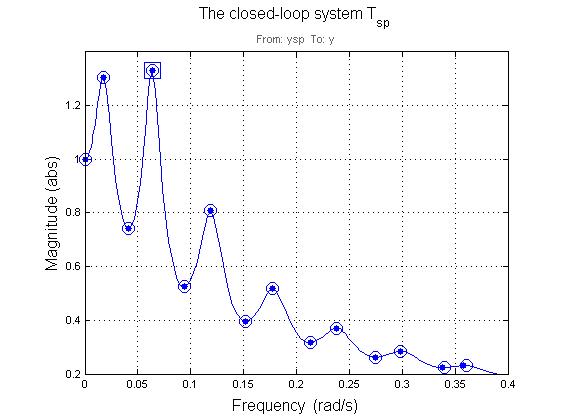
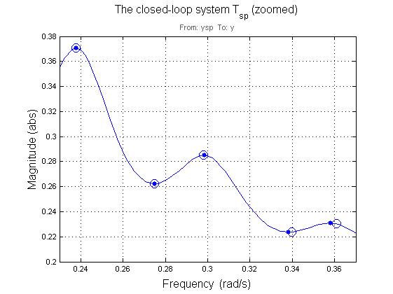
Note that the predicted extremum points do not improve much after correction step for initial points since the approximation in the prediction step reliably computes the points. As shown in Figure 2 at the bottom, zoomed to larger frequencies, we see the improvement in the correction step due to slight deviation of the approximation from the exact values. The closed-loop system is a retarded time-delay system and its asymptotic transfer function is equal to zero which can be seen from the high frequency behavior in Figure 2. Therefore, the strong $\mathcal{H}_{\infty}$ norm of $T_{sp}$ is equal to the standard $\mathcal{H}_{\infty}$ norm of $T_{sp}$ by (39). The norm is equal to the largest singular value $1.3308$ of $4^{th}$ point in the extremum points. This example has a singular $E$ matrix, therefore, the algorithm in [12] is not applicable. When we compared the prediction steps of our algorithm (including pole, zero computation of $G_{N}$) and the one in [9], the computation time is $0.1885$ and $0.6447$ seconds on Intel Xeon $3.06$GHz with $12$GB RAM. The size of the (single) eigenvalue problem for our algorithm is $175$, whereas the size of the eigenvalue problem in [9] is $2n(N+1)=378$ (to be solved in every iteration).

Note that the high frequency behavior in Figure 3 on the top does not converge to zero. Therefore, the asymptotic transfer function is different from zero. As a first step of the algorithm, the strong $\mathcal{H}_{\infty}$ norm of the asymptotic transfer function $T_{a}$, given by

is computed and equals $4$, obtained at $\theta_{1}=0$ and $\theta_{2}=\pi$ in formula (38).

In the second step, we compute the extrema of the magnitude plot by Algorithm 1. The standard $\mathcal{H}_{\infty}$ norm of $T_{sh}$ is equal to $2.5788$ and the high frequency behavior visualized in Figure 3 on the top. Therefore, the strong $\mathcal{H}_{\infty}$ norm of $T_{sh}$ is equal to $4$ by the final step of Algorithm 2, which is larger than the standard $\mathcal{H}_{\infty}$ norm. This illustrates that the $\mathcal{H}_{\infty}$ norm may be sensitive to small delay changes. Figure 3 at the bottom shows that the strong $\mathcal{H}_{\infty}$ norm value $4$ is achieved for a slight perturbation in the delay $\tau_{1}$ and it can be shown that this norm is attained a larger frequency for smaller delay perturbation size.

We presented novel algorithms for the computation of extremal singular values and strong $\mathcal{H}_{\infty}$ norms of SISO time-delay systems described by DDAEs. The latter algorithm does need the iteration inherent to level set methods.

The approach can be easily extended to multi-input-single-output (MISO) and single-input-multiple-output (SIMO) systems. The algorithm namely relies on the property that the singular value plot of the transfer function involves one singular value curve. Whether the presented approach can be extended to general MIMO systems is an open problem.

This work has been supported by the Belgian Federal Science Policy Office, the KU Leuven research council and the Research Foundation-Flanders (FWO). The first author thanks Elfin D. Gumussoy for the fruitful discussions.

References

- [1] S. Boyd and V. Balakrishnan. A regularity result for the singular values of a transfer matrix and a quadratically convergent algorithm for computing its -norm. Systems & Control Letters, 15:1–7, 1990.
- [2] S. Boyd, V. Balakrishnan, and P. Kabamba. A bisection method for computing the norm of a transfer matrix and related problems. Mathematics of Control, Signals and Systems, 2:207–219, 1989.
- [3] D. Breda, S. Maset, and R. Vermiglio. Pseudospectral differencing methods for characteristic roots of delay differential equations. SIAM Journal on Scientific Computing, 27(2):482–495, 2005.
- [4] D. Breda, S. Maset, and R. Vermiglio. Pseudospectral approximation of eigenvalues of derivative operators with non-local boundary conditions. Applied Numerical Mathematics, 56(3-4):318–331, 2006.
- [5] N.A. Bruinsma and M. Steinbuch. A fast algorithm to compute the -norm of a transfer function matrix. Systems & Control Letters, 14:287–293, 1990.
- [6] R. Byers. A bisection method for measuring the distance of a stable matrix to the unstable matrices. SIAM Journal on Scientific and Statistical Computing, 9(9):875–881, 1988.
- [7] P. Gahinet and L. F. Shampine. Software for modeling and analysis of linear systems with delays. In Proceedings of the American Control Conference, 2004.
- [8] S. Gumussoy, B. Eryilmaz, and P. Gahinet. Working with time-delay systems in MATLAB. In 10th IFAC Workshop on Time Delay Systems, Northeastern University, USA, June 22-24 2012.
- [9] S. Gumussoy and W. Michiels. Fixed-order H-infinity control for interconnected systems using delay differential algebraic equations. SIAM Journal on Control and Optimization, 49(2):2212–2238, 2011.
- [10] J.K. Hale and S.M. Verduyn Lunel. Strong stabilization of neutral functional differential equations. IMA Journal of Mathematical Control and Information, 19:5-23, 2002.
- [11] W. Michiels. Spectrum based stability analysis and stabilization of systems described by delay differential algebraic equations. IET Control Theory and Applications, 5(16):1829–1842, 2011.
- [12] W. Michiels and S. Gumussoy. Characterization and computation of H-infinity norms of time-delay systems. SIAM Journal on Matrix Analysis and Applications, 31(4):2093–2115, 2010.
- [13] C.W. Scherer and S. Weiland. Linear Matrix Inequalities in Control. In W.S. Levine (Ed.), The Control Systems Handbook, 2nd Ed., CRC Press, 2010.
- [14] S. Skogestad and I. Postlethwaite. Multivariable Feedback Control. John Wiley, 1996.
- [15] K. Zhou, J.C. Doyle, and K. Glover. Robust and optimal control. Prentice Hall, 1995.