Heterogeneity Pursuit for Spatial Point Pattern with Application to Tree Locations: A Bayesian Semiparametric Recourse
Abstract
Spatial point pattern data are routinely encountered. A flexible regression model for the underlying intensity is essential to characterizing the spatial point pattern and understanding the impacts of potential risk factors on such pattern. We propose a Bayesian semiparametric regression model where the observed spatial points follow a spatial Poisson process with an intensity function which adjusts a nonparametric baseline intensity with multiplicative covariate effects. The baseline intensity is piecewise constant, approached with a powered Chinese restaurant process prior which prevents an unnecessarily large number of pieces. The parametric regression part allows for variable selection through the spike-slab prior on the regression coefficients. An efficient Markov chain Monte Carlo (MCMC) algorithm is developed for the proposed methods. The performance of the methods is validated in an extensive simulation study. In application to the locations of Beilschmiedia pendula trees in the Barro Colorado Island forest dynamics research plot in central Panama, the spatial heterogeneity is attributed to a subset of soil measurements in addition to geographic measurements with a spatially varying baseline intensity.
Keywords— MCMC Powered Chinese Restaurant Process Variable Selection
1 Introduction
Spatial point pattern data, which are random locations of certain events of interest in space (Diggle 2013, e.g.,), arise routinely in many field. Such pattern can be, for example, locations of basketball shooting attempts in sports analytic (Miller et al. 2014; Jiao et al. 2019), earthquake centers in seismology (Schoenberg 2003), or tree species in forestry (Leininger and Gelfand 2017; Thurman and Zhu 2014). Often times, spatially varying covariates are available for characterizing the occurrence of the events. Our motivating application is the spatial point pattern of one of the most common tree species, Beilschmiedia pendula, in the 50–hectare tropical forest dynamics plot at the Barro Colorado Island (BCI) in central Panama (Condit et al. 2019). The BCI data is a great resource for many environmental studies, containing so far complete information of over individual trees that have been censused since the 1980s. It is of interest to characterize the heterogeneity in the distribution of the tree species by both spatially varying covariates and a spatially varying baseline intensity.
Various spatial point process models have been proposed, most of which allow heterogeneity introduced by covariates. Examples are Poisson processes (Yue and Loh 2011), Gibbs process (Dereudre 2019), pairwise interaction models (Baddeley and Turner 2000), Neyman–Scott cluster models (Waagepetersen 2007), log-Gaussian Cox processes (LGCP) (Thurman et al. 2015; Miller et al. 2014), and modified Thomas processes (Yue and Loh 2015), among others. When likelihood estimation is infeasible, estimation can be done based on pseudo-likelihood (Baddeley and Turner 2000). Nonparametric approaches such as kernel and local likelihood have also been proposed for their flexibility (Baddeley et al. 2012). When there are a large number of covariates, regularized estimation has been proposed (Thurman and Zhu 2014; Yue and Loh 2015; Thurman et al. 2015).
Bayesian approaches have been applied to model spatial point processes. The empirical Bayes method has long been used, for example, for inferences for LGCP model parameters (Møller et al. 1998). Full Bayesian approaches have been proposed for various models such as Gibbs processes (Møller et al. 2006; Berthelsen and Møller 2006; King et al. 2012), LGCPs (Møller et al. 1998; Illian et al. 2012), and sequential point processes (Møller and Rasmussen 2012). Specifically, Poisson process models are attractive with a rich range of specifications for the intensity (Kottas and Sansó 2007; Taddy 2010; Yue and Loh 2011, e.g.,). For instance, flexible nonparametric intensities with a piecewise constant surface can be modeled by a mixture of finite mixtures (Geng et al. 2019). Model criticism and model comparison can be based on posterior predictive samples (Leininger and Gelfand 2017).
The focus of this paper is a Bayesian semiparametric spatial Poisson point process model which allows nonparametric spatially varying baseline heterogeneity in addition to covariate-induced heterogeneity. The nonparametric baseline intensity takes the form of a spatially piecewise constant function as in Geng et al. 2019. The Bayesian framework provide naturally estimates for the number of components of the piecewise constant function and the component configuration, along with an estimate of the intensity function itself. In practice, a widely used Dirichlet process, namely the Chinese restaurant process (CRP) (Pitman 1995; Neal 2000) for nonparametric modeling has been reported to produce overly small and, hence, redundant components, making the estimator for the number of components inconsistent (Miller and Harrison 2013). To remedy the situation, Miller and Harrison 2018 put a prior on the number of componentson, resulting a mixture of finite mixtures model; Xie and Xu 2019 developed a general class of Bayesian repulsive Gaussian mixture models to encourage well-separated components. A recent alternative method is the powered Chinese restaurant process (PCRP) (Lu et al. 2018), which encourages member assignment to existing components. The PCRP method has not been used in the context of spatial Poisson point process modeling with a nonparametric baseline as well as covariate effects.
Our contribution is two-fold. First, we propose a flexible Bayesian semiparametric spatial Poisson point process model. The model simultaneously captures the heterogeneity introduced by a spatially varying baseline intensity and the heterogeneity explained by covariates. The baseline intensity is spatially piecewise constant with a PCRP prior, which prevents overfitting. Variable selection is achieved with spike-slab priors (Ishwaran and Rao 2005) on the regression coefficients. The second contribution is an efficient companion Markov chain Monte Carlo (MCMC) inference. The full conditional distribution of the index vector of the grid boxes on the study region under the PCRP prior is summarized in a proposition. The selection of the power of the PCRP prior is done with a criterion similar to the Bayesian information criterion. Our simulation study shows that the proposed method is competitive when the number of data points in each component is sufficiently large. Interesting patterns of the Beilschmiedia pendula species in the BCI plot are discovered.
The rest of this paper is organized as follows. The hierarchical semiparametric model including the spike-slab prior for variable selection is proposed in Section 2. Details of Bayesian methods for the model such as the MCMC algorithm, post MCMC inference for the nonparametric baseline, and selection of the hyperparameter of the PCRP are presented in Section 3. A simulation study is reported in Section 4, followed by an application to the point pattern of Beilschmiedia pendula from the BIC data in Section 5. A discussion concludes in Section 6. Additional technical details are relegated to the Supplementary Materials.
2 Model Setup
2.1 Spatial Poisson Point Process
The spatial Poisson point process is a fundamental model for spatial point patterns. Let be the observed points over a study region with , . A spatial Poisson point process is the process such that the number of points in any subregion follows a Poisson distribution with mean for some function . Function is the intensity function that completely characterizes the spatial Poisson point process. When changes with , the process is known as a non-homogeneous Poisson Point process (NHPP), denoted by .
Covariates can be introduced to the intensity function of a NHPP. Let be a spatially varying covariate vector, which does not include 1. A semiparametric regression model for the intensity function of an NHPP is
| (1) |
where is an unspecified baseline intensity function, and is a vector of regression coefficients. The baseline intensity function captures additional spatial heterogeneity that are not explained by the covariates.
2.2 Nonparametric Baseline Intensity
The baseline intensity function is completely unspecified in Model (1). For flexibility, we characterize by a piecewise constant function
where is the number of components of the piecewise constant function, vector is the unique value of , and is the index of the component at location . In implementation, we partition by disjoint grid boxes , , . Let be the index of the component in the piecewise constant function to which returns for any ; that is, for any , we have .
We specify the index process by a PCRP (Lu et al. 2018). In particular, let and, for ,
| (2) |
where , , and is the number of grid boxes in component . This process is denoted by . The special case of is the CRP. When , the PCRP process assigns , , to an existing component with a higher probability than does the CRP process. This design helps to eliminate artifactual small components produced by the CRP in modeling mixtures with an unknown number of components (Lu et al. 2018). As increases, the probability of each grid box being assigned to an existing component increases so that the final number of components needed decreases.
2.3 Hierarchical Semiparametric Regression Model
With following an NHPP and index vector following a PCPR, the proposed hierarchical semiparametric regression model denoted by PCRP-NHPP is
| (3) |
where ; and are defined in (1) and (2), respectively, with hyperparameters and a pre-specified power for the PCRP; the prior distributions for ’s are independent; the prior distributions for ’s are independent gamma distributions with mean ; and is the number of unique values of .
When variable selection is desired, a spike-slab prior can be imposed on each element of (Ishwaran and Rao 2005). A spike-slab distribution is a mixture of a nearly degenerated distribution at zero (the spike) and a flat distribution (the slab). Zero-mean normal distributions with a small and a large variance are common choices, respectively, for the spike and the slab. The ratio of the two variances should be in a reasonable range such that the MCMC will not get stuck in the spike component (Malsiner-Walli and Wagner 2018). Following the suggestion from George and McCulloch 1993, a common choice of the two variances are 0.01 and 100. Specifically, the normal spike-slab prior specifies the hyperparameter , , in (3) as
| (4) | ||||
With posterior samples from MCMC, variable selection is done using the posterior modes of ’s. A posterior mode zero of suggests little significance of and exclusion of the corresponding covariate from the regression model.
3 Bayesian Inference
3.1 The MCMC Sampling Scheme
The parameters in Model (3)–(4) are , where . The likelihood of spatial Poisson point process is
The posterior density of is
where is the prior density of .
The full conditional distribution of each parameter in are derived in order to use Gibbs sampling method; see Section A in the Appendix. The full conditional distribution for the elements in the index process is summarized in the following Proposition.
Proposition 1
Under the model and prior specification (3), the full conditional distribution of , , is
| (5) |
where is with removed, is the number of grid boxes in component excluding , is the number of data points in grid box , and , The results remain when the spike-slab prior is imposed on the elements of .
Assuming that the covariates are piecewise constant on a grid partition, which may not be the same as the ’s, the integral of in Proposition 1 can be calculated as a summation on each , . If this grid partition is the same as ’s, that is, for , then , where is the area of .
The full conditional distributions for ’s and ’s are straightforward from their conjugate priors:
| (6) | ||||
| (7) |
where and are, respectively the and without the th element, is the number of data points in the component, and is the density of .
The full conditional density of , is proportional to
| (8) |
where is without the th element. The Metropolis–Hastings algorithm (Hastings 1970) can be used to draw samples from this conditional distribution. In our implementation, we used a normal distribution proposal centered at the current value with a standard deviation that is tuned to achieve a desired acceptance rate.
The full conditional distributions facilitate MCMC sampling with an Gibbs sampling algorithm. Algorithm 1 summarizes the specifics for one MCMC iteration. In the algorithm, , the length of , reduces by 1 whenever a component is found to contain only a single grid box; it increases by 1 when a new label is assigned by the full conditional distribution (5). To initialize, each , , is randomly assigned an integer value in for a prespecified initial number of components for the piecewise constant baseline, possibly based on some exploratory analysis. Initial values for are generated independently from the prior distribution. Initial values for other parameters and can simply be set to zeros.
3.2 Inference for the Nonparametric Baseline Intensity
Bayesian inference for the nonparametric baseline intensity is not as straightforward as for the regression coefficients whose posterior sample can be easily summarized. The nonparametric baseline intensity is constructed based on the index vector , which can not be summarized using traditional posterior mean or mode. The same value from different iterations does not necessarily mean the same component. The similar problem also exists in inference of . We use Dahl’s method (Dahl 2006) as a simple solution for summarizing . It chooses the iteration in the posterior sample that optimizes a least squares criterion as the estimate for .
For a draw from the posterior distribution of , define an membership matrix
| (9) |
That is, its -th element is 1 if the -th and -th grid boxes belong to the same component (or have the same baseline intensity); it is 0 otherwise. For an MCMC sample of size , let be the matrix defined for the th draw in the sample and . Then each -th element of is the relative frequency that the -th and -th grid boxes belong to the same component. Dahl 2006 suggested to take the draw in the sample that is closest to as the point estimate of . Let
The estimate for is and the estimate of is the length of . The advantage of this method is that is uses information from all posterior samples, and the final result is guaranteed to be a valid scheme that exists in the sample.
Convergence check for the nonparametric baseline cannot be done with trace plots for or as their meanings change from iteration to iteration. The baseline at each grid box, , , does have the same meaning across iteration and can be checked for convergence. The situation is similar to that of a reversible jump MCMC where a nonparametric component has varying degrees of freedom (Wang et al. 2013). Instead of monitoring a large number grid boxes, we focus on the number of component in practice and monitor the trace plot of for stationarity. Usually, once shows stationarity, the nonparametric baseline at each grid box and the regression coefficients are all stationary.
As a further diagnostic tool for the nonparametric baseline, the Rand index (RI), which measures the similarity of two component memberships (Rand 1971), can be checked. Let be the collection of all pairs of grid boxes. For two index vectors and , define
where denotes the cardinality of a set. That is, under the two membership assignments, and are the number of grid box pairs whose memberships are “concordant”; other pairs are all “discordant”. Then, RI is defined as
which ranges from 0 to 1 with a higher value indicating a better agreement between the two index vectors, and 1 indicates a perfect match.
If the true index vector were known, for every MCMC iteration , , a Rand index based on and can be calculated. The trace plot of is a useful diagnostic tool. In practice, since is unknown, we replace it with the estimate from Dahl’s method after convergence has been ensured from the trace plot of . The stationarity in the trace plot of RI provides a second stage reassurance of the convergence, and its level provides a measure for the quality of the consistency of the memberships from iteration to iteration.
3.3 Selection of
The estimated number of components of the nonparametric baseline intensity depends on , the power of the PCRP prior. Selection of remains to be addressed. Model comparison criteria under the Bayesian framework, such as deviance information criterion (DIC) (Spiegelhalter et al. 2002) and logarithm of pseudo-marginal likelihood (LPML) (Geisser and Eddy 1979; Gelfand and Dey 1994), are natural choices. From our simulation study, however, they tended to lead to overestimation of the number of components in the nonparametric baseline. We experimented with a criterion in the spirit of the Bayesian information criterion (BIC) since BIC has proven to be an effective criterion for likelihood-based model selection in clustering algorithms (Wang and Bickel 2017).
Our Bayesian information type criterion (BITC) is defined as
| (10) |
where and are estimator of and , respectively, from Dahl’s method. Although BIC is usually used for frequentist methods, when number of points and the MCMC sample size are large enough, provides a consistent estimator of (Walker 1969) and it is reasonable to use BITC to assess model fitting without considering parameter variation. The effectiveness of the BITC in selecting was confirmed in our simulation study reported in the next section. In practice, we can determine the range of candidate values starting from 1 and ending with a number that gives . Then the optimal is selected based on the BITC from a grid of candidate values. The optimal selected by this criterion provided better estimate of in our simulation than those by LPML and DIC. Its performance in general model comparison is beyond the scope of this paper.
4 Simulation Study
The proposed methods were validated in a simulation study over a region . The study region is partitioned by grid boxes , , where each , , is a unit square. Points were generated from the model (1) with covariates. The four covariates , , were set to be piecewise constant over the grid boxes ’s. Their values were independently generated from the standard normal distribution. The true regression coefficients were and . Two settings of the piecewise constant baseline intensity surface were considered. Setting 1 had two components, with , and the number of grid boxes in the two components were . Setting 2 had three components, with , and . See Figure 5 for the spatial structure of the baseline intensity surfaces under the two settings. In both settings, more grid boxes were assigned to first component with low intensity value, which mimics the pattern of the BCI data. We used function rpoispp() from R package spatstat (Baddeley et al. 2015) to generate the points. For each setting, 100 replicates were generated. There were about to data points generated under setting 1, and about to data points generated under setting 2.
Priors for the model parameters were set to be those in (3) and (4), with hyperparameters . Different values starting from 1 were tried on each dataset and the optimal was selected by the BITC in (10). The upper end of the candidate in each setting was experimented to be the smallest value that would lead to a single component of the piecewise constant baseline intensity surface based on Dahl’s method. Candidate powers used for setting 1 were from 1 to 2 with a step 0.1; for setting 2, candidate powers used were from 1 to 3 with a step 0.1. In the Metropolis–Hastings algorithm to draw , a Normal distribution was used as the proposal, which yielded an acceptance rate of 30–40%. For each dataset, we ran the MCMC for 5000 iterations and discarded the first 1000 iterations. Convergence for the remaining iterations was ensured by checking the trace plots of the elements in and .
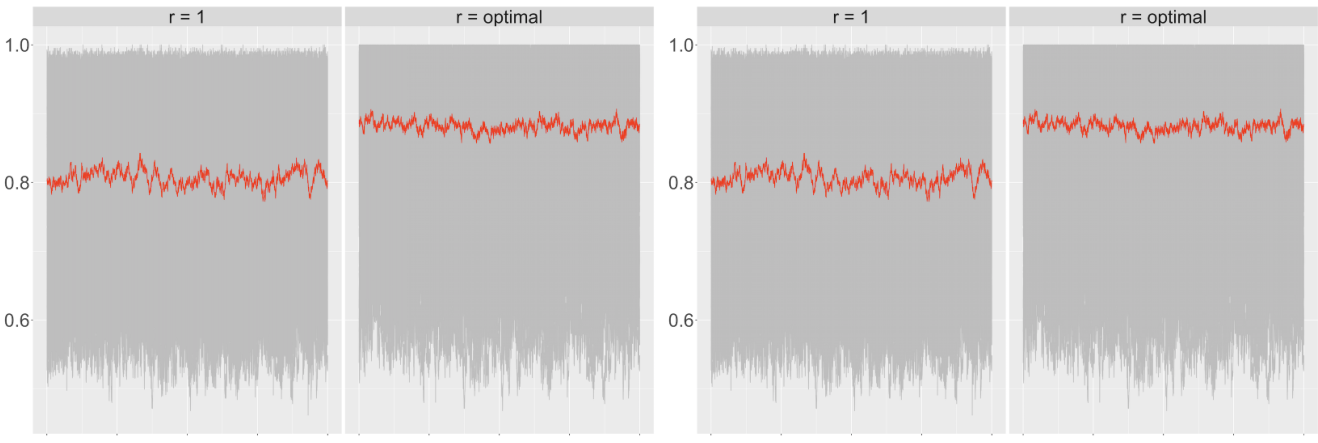
Figure 1 shows the histograms of from Dahl’s method for a selective set of values based on the 100 replicates. The optimal was selected by the BITC. The true are 2 and 3, respectively, in the two settings. The histograms of under the optimal are much closer to the true under both settings than those under , the popular CRP prior. Among the 100 replicates, there are 76 times in setting 1 and 84 times in setting 2 that the optimal led to exactly. The same frequencies for are only 55 and 18, respectively. LPML and DIC were also calculated using the Monte Carlo estimation proposed by Hu et al. 2019. As shown in Figure 6, they had good performance under setting 1, estimating correctly for 81 times and 83 times, respectively. Nonetheless, both of them did fairly poorly under setting 2 with obviously more components estimated than the truth. Only 24 times and 23 times out of the 100 replicates estimated correctly using LPML and DIC, respectively.
Also shown in Figure 1 are the overlaid trace plots of the RI from all the replicates under and the optimal . The trace plots further assure the convergence of the index process in the sense of Rand 1971. The averaged trace plots over the replicates (shown in solid lines) reflect the level of consistency in component memberships across iterations. Under , the averages stabilize around 0.806 and 0.828, respectively, for setting 1 and setting 2. Under the optimal , the averages are 0.882 and 0.893, respectively, indicating higher consistencies in component membership than those under .
The estimated baseline intensity surfaces under the optimal for the 100 replicates are summarized, and the heat maps of their percentile, median and percentile are compared with the true surface in Figure 5. According to the plots, fitted baseline intensity can accurately specify different components, and the intensity magnitude is also very close to the truth. The estimation of the edge part of different components do not show obvious worse performance. This is because PCRP does not have spatial smoothness constraint and allows more spatial flexibility. As long as the resolution of grid box is fine enough, PCRP can capture different components no matter the shape of the area. Under each setting, we pool the grid boxes under the same component and compare the averaged estimates with the true value. For setting 1, the empirical biases for the two components of are , with standard deviations . For setting 2, the empirical biases for the three components are , with standard deviations . Considering the magnitude of the intensity components, they are estimated quite accurately.
| Setting | AR() | Bias | SD | ||
|---|---|---|---|---|---|
| Setting 1 | 0.5 | 100 | 0.019 | 0.035 | 0.033 |
| 0.5 | 100 | 0.016 | 0.032 | 0.033 | |
| 0.0 | 100 | 0.028 | 0.034 | 0.030 | |
| 0.0 | 100 | 0.022 | 0.035 | 0.031 | |
| Setting 2 | 0.5 | 100 | 0.012 | 0.027 | 0.026 |
| 0.5 | 100 | 0.011 | 0.025 | 0.025 | |
| 0.0 | 100 | 0.007 | 0.024 | 0.023 | |
| 0.0 | 100 | 0.003 | 0.021 | 0.023 |
Table 1 summarizes the results of variable selection and estimation for the parametric regression part of the model. For both settings, the two important variables were included and the two unimportant variables were excluded with accuracy rate 100%. The empirical bias of the coefficients are minimal. The empirical standard errors of the point estimates have good agreement with the average of the posterior standard deviation of the coefficients. The variation of the coefficient estimates is lower in setting 2 than in setting 1, which is expected because setting 2 has high intensity and more observed points.
Finally, the proposed model was compared with three competing models. The first one, denoted as “const-NHPP”, is the model (1) with a constant baseline intensity surface . The second one, denoted as “spline-NHPP”, is the model (1) with baseline intensity surface approximated by a tensor product cubic splines with a single knot for each of the two coordinates (Berhane et al. 2008, e.g.,). This model can be fit with the spline basis into the covariates. The last model is the LGCP model fitted with function kppm() from R package spatstat (Baddeley et al. 2015). The mean squared error (MSE) is often used to compare the performances of different models in modeling spatial point pattern, which, with a grid partition ’s on , is defined as
| (11) |
where , is the estimated intensity on location . Models with smaller MSE values are preferred.
Figure 2 summarizes the boxplots of the MSE across the proposed model and the three competing models. The three competing models are all misspecified under the data generating schemes. As expected, they have much higher MSEs than the proposed model. In particular, the const-NHPP and LGCP models show very similar results, since the LGCP model mainly makes improvements on the intensity’s variance structure, which does not help here. The MSE of the spline-NHPP model could be further reduced if more flexibility in the splines were introduced. Nonetheless, its baseline intensity is spatially continuous which may never fit well the data generated in our settings with piecewise constant intensity surface consisting of only two or three quite different components.
5 Point Pattern of Beilschmiedia Pendula
Beilschmiedia pendula is one of the most abundant tree species in the BCI (Thurman and Zhu 2014). There are such trees in total from the most recent census in the 50-hectare plot , a rectangle of . Their exact locations are recorded in a Cartesian coordinate system ; see Figure 3. In addition to two geographical variables, elevation and slope, thirteen environmental covariates are available, which are soil pH and concentrations in the soil of aluminum (Al), boron (B), calcium (Ca), cuprum (Cu), ferrum (Fe), kalium (K), magnesium (Mg), manganese (Mn), phosphorus (P), zinc (Z), nitrogen (N), and nitrogen mineralization (N.min.). The latest version of these covariates data was from 2004, available at http://ctfs.si.edu/webatlas/datasets/bci/soilmaps/BCIsoil.html, These variables were measured at each of the grid boxes of size over . Within each grid box, the measures are assumed to be the same so that each measure is piecewise constant over . The heat maps of the standardized covariates are also shown in Figure 3.

With standardized covariates, the hierarchical semiparametric model (3)–(4) were fit to the observed point pattern of Beilschmiedia Pendula. For better numerical performance, the area of each grid box was scaled to be 1. The hyperparameters were set to be . The standard deviation of the normal proposal in the Metropolis–Hastings algorithm was set to be 0.05 in order to make the acceptance rate between and . A grid of values were used for in search for an optimal . For each , an MCMC was carried out for 50,000 iteration. The first 10,000 iterations dropped as burnin, and the remaining iterations were thinned by 10, yielding an MCMC sample of size . The convergence was checked for the trace plots of and ; see Figure 7.
The optimal was selected to be 1.3 by the BITC, which leads to from Dahl’s method. The posterior mode of is also 4, with a frequency of 1198 out of 2000. The posterior standard deviation of is 0.852. About 93.4% of the sample values of are , which is rather tight compared to those from the CRP prior for the baseline (). The average RI over the MCMC sample was 0.806, suggesting good concordance of the component assignments over the MCMC iterations. The four baseline intensity estimates are 0.880, 4.983, 13.182, and 28.059, which are well separated, representing low, moderate, high, and extremely high components, respectively. The posterior median of the surface of the baseline intensity over the study plot, as well as the 2.5% and 97.5% percentiles, are shown in Figure 4. Clearly, after accounting for the available covariates, there are missing covariates that could have helped to explain the distribution of the tree species, but they are now captured by the nonparametric baseline intensity.

Table 2 summarizes the posterior mean, standard deviation, and the 95% highest posterior density (HPD) credible intervals of the regression coefficients. Also reported is the posterior probability of for each covariate , which was used to decide whether the corresponding covariate is important. The covariates that are selected are marked with a star symbol “*”. The HPD intervals for those covariates that are not selected either cover 0, or are very close to 0. The tree species appears to prefer places with higher elevation and steeper slope, which agrees with the results in Thurman and Zhu 2014. More occurrence of the species is associated with higher concentrations of Al and Ca, and lower concentrations of Fe, K, P, and Zn in the soil. These factors’ influences on this specific tree species have not been measured quantitatively before using the BCI dataset.
| Covariate | Posterior | Estimate | SE | 95% HPD Credible Interval |
|---|---|---|---|---|
| elevation | 1.000* | 0.694 | 0.065 | ( 0.575, 0.822) |
| slope | 1.000* | 0.651 | 0.039 | ( 0.570, 0.727) |
| pH | 0.015 | 0.063 | 0.052 | (, 0.156) |
| Al | 0.959* | 0.503 | 0.089 | ( 0.323, 0.671) |
| B | 0.014 | 0.067 | (, 0.085) | |
| Ca | 1.000* | 0.991 | 0.110 | ( 0.765, 1.203) |
| Cu | 0.020 | 0.073 | 0.068 | (, 0.198) |
| Fe | 0.543* | 0.110 | (, ) | |
| K | 0.817* | 0.121 | (, ) | |
| Mg | 0.032 | 0.078 | 0.075 | (, 0.222) |
| Mn | 0.117 | 0.187 | 0.064 | ( 0.064, 0.309) |
| P | 0.915* | 0.070 | (, ) | |
| Zn | 0.678* | 0.105 | (, ) | |
| N | 0.019 | 0.052 | (, 0.005) | |
| N.min | 0.021 | 0.063 | 0.061 | (, 0.173) |
We also fitted other three competing models in the simulation study and compared the MSE of the models calculated on the grid. In the spline-NHPP model, cubic B-spline basis were used with three knots for and one knot for , since the range of is twice as long as that of , resulting 7 and 5 degrees for and , respectively, in the tensor product spline basis construction. The proposed method gives an MSE of only 6.00. The MSE from the const-NHPP, spline-NHPP, and LGCP models are 26.69, 19.98 and 26.70, respectively. The improvement made by the proposed method is obvious.
6 Discussion
Explaining the spatial heterogeneity of point patterns is challenging when important covariates are not observed. The proposed semiparametric NHPP model captures the heterogeneity unexplained by observed covariates with a spatially varying baseline intensity. The baseline intensity surface is of a flexible form of piecewise constant on a grid partition of the study region, with a PCRP prior that prevents overly small components often seen when a CRP prior is imposed instead. The methodology is particularly useful when the baseline intensity surface lacks smoothness as in the case of missing covariates. The fitted number of components of the piecewise constant baseline depends on the power of the PCRP. The selection of thorough the BITC specifically designed for this setting seems to be more effective in the simulation study than the LPML and DIC.
A few topics beyond the scope of this paper merits further investigation. When the baseline intensity is deemed to be spatially contiguous, imposing spatial contiguity on the piecewise constant intensity surface (Li and Sang 2019) may lead to more efficient estimator of the surface. Some applications may have large areas containing no events, in which case, including zero-inflated structures (Lambert 1992) in spatial point process models may improve the fitting and avoid unidentifiably close-to-zero intensities. Finally, selection of for the PCRP prior by the BITC needs to be evaluated in more general settings. A tuning-free strategy, for example, through a hyper prior on , would be desirable for practice.
Acknowledgements
The authors thank Drs. Dipak Dey and Yishu Xue for their comments and suggestions. GH’s research was supported by Dean’s office of the College of Liberal Arts and Sciences at the University of Connecticut. The BCI forest dynamics research project was founded by S.P. Hubbell and R.B. Foster and is now managed by R. Condit, S. Lao, and R. Perez under the Center for Tropical Forest Science and the Smithsonian Tropical Research in Panama. Numerous organizations have provided funding, principally the U.S. National Science Foundation, and hundreds of field workers have contributed.
Supporting Information
Appendix A
This section shows the derivation of full conditionals needed for the MCMC. For the full conditional distribution of , we only need to focus on those data points that are in the th component since the likelihood for the data points in other components does not involve . That is, we only need to focus on those grid boxes ’s such that . The full conditional density of , , is
| (12) | ||||
which is the density of .
The full conditional mass function of , , is
| (13) |
which is Bernoulli with rate parameter
The full conditional density of , , is
| (14) |
This is not a standard distribution. Sampling from it can be done with a Metropolis–Hasting algorithm with a normal proposal distribution centered at the value of the current iteration with a variance parameter tuned to achieve desired acceptance rate.
The full conditional distribution of , , is contingent on whether the th grid box goes to an existing component or a new one (Neal 2000). The full conditional probability that grid box belongs to an existing component , i.e., , is
| (15) | ||||
The full conditional probability that belongs to a new component, i.e., , is
| (16) | ||||
Combining (15) and (16) gives the full conditional distribution of in the main text.
Appendix B
This section includes supporting materials for simulation study. There are two different settings for baseline intensity in simulation study. The heatmaps showing the configuration of baseline intensity surfaces, and the fitted surfaces corresponding to the quantile, median and quantile of 100 replicates are displayed in Figure 5.


The performances of LPML and DIC to select power are not good. The have satisfying results under setting 1, where most of the time they give correct estimation for , but under setting 2, when the problem is more difficult, both of them fail to give accurate estimate for . The histgrams of chosen by LPML and DIC over 100 replicates are shown in Figure 6.
Appendix C
The trace plots of and for BCI data fitting results after burnin and thinning are shown in Figure 7. The convergence of each element in is satisfying. The trace plot of shows good convergence of the grouping process (Wang et al. 2013). Since Dahl’s method requires that the chain has converged, we first checked the convergence using trace plot of . The estimation for was then calculated using Dahl’s method. It was then used in place of the truth to construct the trace plot of RI, which was used to further check the convergence of .

References
- Baddeley et al. (2012) Baddeley, A., Y.-M. Chang, Y. Song, and R. Turner (2012). Nonparametric estimation of the dependence of a spatial point process on spatial covariates. Statistics and Its Interface 5(2), 221–236.
- Baddeley et al. (2015) Baddeley, A., E. Rubak, and R. Turner (2015). Spatial Point Patterns: Methodology and Applications with R. Chapman and Hall/CRC.
- Baddeley and Turner (2000) Baddeley, A. and R. Turner (2000). Practical maximum pseudolikelihood for spatial point patterns. Australian & New Zealand Journal of Statistics 42(3), 283–322.
- Berhane et al. (2008) Berhane, K., M. Hauptmann, and B. Langholz (2008). Using tensor product splines in modeling exposure–time–response relationships: Application to the Colorado Plateau Uranium Miners cohort. Statistics in Medicine 27(26), 5484–5496.
- Berthelsen and Møller (2006) Berthelsen, K. K. and J. Møller (2006). Bayesian analysis of Markov point processes. In A. Baddeley, P. Gregori, J. Mateu, R. Stoica, and D. Stoyan (Eds.), Case Studies in Spatial Point Process Modeling, pp. 85–97. Springer.
- Condit et al. (2019) Condit, R., R. Perez, S. Aguilar, S. Lao, R. Foster, and S. P. Hubbell (2019). Complete Data from the Barro Colorado 50-ha Plot: 423617 Trees, 35 Years, 2019 Version.
- Dahl (2006) Dahl, D. B. (2006). Model-based clustering for expression data via a Dirichlet process mixture model. In M. V. Kim-Anh Do, Peter Müller (Ed.), Bayesian Inference for Gene Expression and Proteomics, Volume 4, pp. 201–218. Cambridge University Press.
- Dereudre (2019) Dereudre, D. (2019). Introduction to the theory of Gibbs point processes. In D. Coupler (Ed.), Stochastic Geometry, pp. 181–229. Springer.
- Diggle (2013) Diggle, P. J. (2013). Statistical Analysis of Spatial and Spatio-Temporal Point Patterns. Chapman and Hall/CRC.
- Geisser and Eddy (1979) Geisser, S. and W. F. Eddy (1979). A predictive approach to model selection. Journal of the American Statistical Association 74(365), 153–160.
- Gelfand and Dey (1994) Gelfand, A. E. and D. K. Dey (1994). Bayesian model choice: Asymptotics and exact calculations. Journal of the Royal Statistical Society. Series B (Methodological) 56(3), 501–514.
- Geng et al. (2019) Geng, J., W. Shi, and G. Hu (2019). Bayesian nonparametric nonhomogeneous Poisson process with applications to USGS earthquake data. arXiv e-prints 1907.03186.
- George and McCulloch (1993) George, E. I. and R. E. McCulloch (1993). Variable selection via Gibbs sampling. Journal of the American Statistical Association 88(423), 881–889.
- Hastings (1970) Hastings, W. K. (1970). Monte Carlo sampling methods using Markov chains and their applications. Biometrika 57(1), 97–109.
- Hu et al. (2019) Hu, G., F. Huffer, and M.-H. Chen (2019). New development of Bayesian variable selection criteria for spatial point process with applications. arXiv e-prints 1910.06870.
- Illian et al. (2012) Illian, J. B., S. H. Sørbye, and H. Rue (2012). A toolbox for fitting complex spatial point process models using integrated nested Laplace approximation (INLA). The Annals of Applied Statistics 6, 1499–1530.
- Ishwaran and Rao (2005) Ishwaran, H. and J. S. Rao (2005). Spike and slab variable selection: Frequentist and Bayesian strategies. The Annals of Statistics 33(2), 730–773.
- Jiao et al. (2019) Jiao, J., G. Hu, and J. Yan (2019, Aug). A Bayesian Joint Model for Spatial Point Processes with Application to Basketball Shot Chart. arXiv e-prints 1908.05745.
- King et al. (2012) King, R., J. B. Illian, S. E. King, G. F. Nightingale, and D. K. Hendrichsen (2012). A Bayesian approach to fitting Gibbs processes with temporal random effects. Journal of Agricultural, Biological, and Environmental Statistics 17(4), 601–622.
- Kottas and Sansó (2007) Kottas, A. and B. Sansó (2007). Bayesian mixture modeling for spatial Poisson process intensities, with applications to extreme value analysis. Journal of Statistical Planning and Inference 137(10), 3151–3163.
- Lambert (1992) Lambert, D. (1992). Zero-inflated Poisson regression, with an application to defects in manufacturing. Technometrics 34(1), 1–14.
- Leininger and Gelfand (2017) Leininger, T. J. and A. E. Gelfand (2017). Bayesian inference and model assessment for spatial point patterns using posterior predictive samples. Bayesian Analysis 12(1), 1–30.
- Li and Sang (2019) Li, F. and H. Sang (2019). Spatial homogeneity pursuit of regression coefficients for large datasets. Journal of the American Statistical Association. Forthcoming.
- Lu et al. (2018) Lu, J., M. Li, and D. Dunson (2018). Reducing over-clustering via the powered Chinese restaurant process. arXiv e-prints 1802.05392.
- Malsiner-Walli and Wagner (2018) Malsiner-Walli, G. and H. Wagner (2018). Comparing spike and slab priors for Bayesian variable selection. arXiv e-prints 1812.07259.
- Miller et al. (2014) Miller, A., L. Bornn, R. Adams, and K. Goldsberry (2014). Factorized point process intensities: A spatial analysis of professional basketball. In Proceedings of the 31st International Conference on International Conference on Machine Learning - Volume 32, ICML’14, pp. 235–243.
- Miller and Harrison (2013) Miller, J. W. and M. T. Harrison (2013). A simple example of Dirichlet process mixture inconsistency for the number of components. In Proceedings of the 26th International Conference on Neural Information Processing Systems — Volume 1, NIPS’13, USA, pp. 199–206. Curran Associates Inc.
- Miller and Harrison (2018) Miller, J. W. and M. T. Harrison (2018). Mixture models with a prior on the number of components. Journal of the American Statistical Association 113(521), 340–356.
- Møller et al. (2006) Møller, J., A. N. Pettitt, R. Reeves, and K. K. Berthelsen (2006). An efficient Markov chain Monte Carlo method for distributions with intractable normalising constants. Biometrika 93(2), 451–458.
- Møller and Rasmussen (2012) Møller, J. and J. G. Rasmussen (2012). A sequential point process model and Bayesian inference for spatial point patterns with linear structures. Scandinavian Journal of Statistics 39(4), 618–634.
- Møller et al. (1998) Møller, J., A. R. Syversveen, and R. P. Waagepetersen (1998). Log-Gaussian Cox processes. Scandinavian Journal of Statistics 25(3), 451–482.
- Neal (2000) Neal, R. M. (2000). Markov chain sampling methods for Dirichlet process mixture models. Journal of Computational and Graphical Statistics 9(2), 249–265.
- Pitman (1995) Pitman, J. (1995). Exchangeable and partially exchangeable random partitions. Probability Theory and Related Fields 102(2), 145–158.
- Rand (1971) Rand, W. M. (1971). Objective criteria for the evaluation of clustering methods. Journal of the American Statistical Association 66(336), 846–850.
- Schoenberg (2003) Schoenberg, F. P. (2003). Multidimensional residual analysis of point process models for earthquake occurrences. Journal of the American Statistical Association 98(464), 789–795.
- Spiegelhalter et al. (2002) Spiegelhalter, D. J., N. G. Best, B. P. Carlin, and A. Van Der Linde (2002). Bayesian measures of model complexity and fit. Journal of the Royal Statistical Society: Series B (Statistical Methodology) 64(4), 583–639.
- Taddy (2010) Taddy, M. A. (2010). Autoregressive mixture models for dynamic spatial Poisson processes: Application to tracking intensity of violent crime. Journal of the American Statistical Association 105(492), 1403–1417.
- Thurman et al. (2015) Thurman, A. L., R. Fu, Y. Guan, and J. Zhu (2015). Regularized estimating equations for model selection of clustered spatial point processes. Statistica Sinica 25(1), 173–188.
- Thurman and Zhu (2014) Thurman, A. L. and J. Zhu (2014). Variable selection for spatial Poisson point processes via a regularization method. Statistical Methodology 17, 113–125.
- Waagepetersen (2007) Waagepetersen, R. P. (2007). An estimating function approach to inference for inhomogeneous Neyman–Scott processes. Biometrics 63(1), 252–258.
- Walker (1969) Walker, A. M. (1969). On the asymptotic behaviour of posterior distributions. Journal of the Royal Statistical Society: Series B (Methodological) 31(1), 80–88.
- Wang et al. (2013) Wang, X., M.-H. Chen, and J. Yan (2013). Bayesian dynamic regression models for interval censored survival data with application to children dental health. Lifetime Data Analysis 19(3), 297–316.
- Wang and Bickel (2017) Wang, Y. R. and P. J. Bickel (2017). Likelihood-based model selection for stochastic block models. The Annals of Statistics 45(2), 500–528.
- Xie and Xu (2019) Xie, F. and Y. Xu (2019). Bayesian repulsive Gaussian mixture model. Journal of the American Statistical Association. Forthcoming.
- Yue and Loh (2015) Yue, Y. and J. M. Loh (2015). Variable selection for inhomogeneous spatial point process models. Canadian Journal of Statistics 43(2), 288–305.
- Yue and Loh (2011) Yue, Y. R. and J. M. Loh (2011). Bayesian semiparametric intensity estimation for inhomogeneous spatial point processes. Biometrics 67(3), 937–946.