Measurement-Level Fusion for OTHR Network Using Message Passing
Abstract
Tracking an unknown number of targets based on multipath measurements provided by an over-the-horizon radar (OTHR) network with a statistical ionospheric model is complicated, which requires solving four subproblems: target detection, target tracking, multipath data association and ionospheric height identification. A joint solution is desired since the four subproblems are highly correlated, but suffering from the intractable inference problem of high-dimensional latent variables. In this paper, a unified message passing approach, combining belief propagation (BP) and mean-field (MF) approximation, is developed for simplifying the intractable inference. Based upon the factor graph corresponding to a factorization of the joint probability distribution function (PDF) of the latent variables and a choice for a separation of this factorization into BP region and MF region, the posterior PDFs of continuous latent variables including target kinematic state, target visibility state, and ionospheric height, are approximated by MF due to its simple MP update rules for conjugate-exponential models. With regard to discrete multipath data association which contains one-to-one frame (hard) constraints, its PDF is approximated by loopy BP. Finally, the approximated posterior PDFs are updated iteratively in a closed-loop manner, which is effective for dealing with the coupling issue among target detection, target tracking, multipath data association, and ionospheric height identification. Meanwhile, the proposed approach has the measurement-level fusion architecture due to the direct processing of the raw multipath measurements from an OTHR network, which is benefit to improving target tracking performance. Its performance is demonstrated on a simulated OTHR network multitarget tracking scenario.
Index Terms:
Multiple target tracking, measurement-level fusion, over-the-horizon radar network, message passingI Introduction
By exploiting sky-wave propagation via reflection by the ionosphere, an over-the-horizon radar (OTHR) provides detection and monitoring of both air targets and maritime targets beyond the line-of-sight horizon [1]. Due to its cost-effectiveness and the ability to monitor remote geographical regions where conventional line-of-sight radars are not able to cover, OTHR has been received long-standing interest in both defense and civil applications. An OTHR network, such as Australia’s Jindalee Operational Radar Network (JORN) [2], consists of multiple OTHRs that have a degree of overlapping coverage and are operated jointly to achieve overall mission objectives. Compared with a single OTHR, many benefits can be achieved through fusing all the information from an OTHR network: (1) Improved target detection: Target detection ability of an OTHR is related to the fading characteristics of ionosphere and the Doppler speed of a target. Multiple and independent OTHRs have different ionospheric fading patterns and geometric positions relating to the target. Therefore, integrating the information from an OTHR network can improve detection probability of the target, and this also benefits to increasing the timeliness of initializing tracks. (2) Improved target tracking: Once target detection probability is improved, target track detection probability and stability of target tracking will be improved as well. Moreover, redundant data from an OTHR network increases target track accuracy by providing independent observations of the target. (3) Better coordinate registration (CR): Improved target track accuracy can aid in resolving ambiguities and uncertainties in the decision of multipath data association 11 1 There are two types of association in OTHR, i.e., data association due to multiple targets scenario and path association arising from multipath propagation. We call the target-to-measurement-to-path association as multipath data association. and the identification of ionospheric height.
However, because of the ionosphere, which is complex in nature, difficulties arise from both continuous and discrete uncertainties for an OTHR network fusion: (1) CR uncertainty: CR uses available information on ionosphere, including propagation paths and corresponding ionospheric heights, to localize a target by converting observations of the target in radar slant coordinate systems to ground or geographic coordinate systems. However, high-frequency signal propagation through separate refractive layers in the ionosphere often results in multiple propagation paths/modes between a target and an OTHR, producing multiple resolved (multipath) measurements of the target with a high probability. Accordingly, path/mode association ambiguity occurs in CR. Moreover, ionospheric heights vary spatially and temporally, adding an extra degree of uncertainty to CR. If the propagation path is not selected correctly and/or ionospheric heights are not estimated precisely, the ground track of a target will be inaccurate and it will be difficult to correlate the ground tracks from multiple OTHRs. (2) Data association uncertainty: The OTHR performance characteristics are indicated by poor measurement accuracy, long sampling period, low detection probability (per path), and high false-alarm rate, complicating the data association. In a single OTHR tracker, ghost tracks will arise if multipath measurements are not be associated correctly with the underlying target in the tracking stage, or multipath tracks are not be fused correctly at the post-tracking stage. This problem is exacerbated when an unknown number of targets are tracked in an OTHR network.
Achieving multitarget tracking by fusing unlabeled multipath measurements from an OTHR network, requires solving four subproblems: target detection, target tracking, multipath data association, and ionospheric height identification. Most existing target tracking algorithms are only applicable to a single OTHR. The multipath track fusion algorithm (MPTF) [3] reflects the view that tracking and fusion are two-stage process whereas the first-stage tracking process produces the multipath slant tracks independently, and the second-stage fusion process associates those slant tracks and fuse them. Multipath measurement fusion approaches [4, 5, 6, 7, 8, 9, 10, 11] integrate tracking and fusion as a single, unified process. By extending the existing data association approach to multipath data association, the target tracks in ground coordinate systems are updated directly using multipath measurements.
Extending MPTF for a single OTHR to multiple OTHRs (MR-MPTF), the work of [12, 13] studied fusion for an OTHR network. Based on (slant) track-level fusion framework, MR-MPTF treats target tracking and multiple radar fusion as two independent processes. Specifically, MR-MPTF carries out single-path target tracking in radar slant coordinate system for each OTHR, generates multiple feasible association hypotheses using all possible combinations of existing ionospheric paths, transform the relevant multipath tracks from multiple OTHRs into a common coordinate system whereas all track-to-target association hypotheses are recursively constructed, and then fuse target states with the weight given by the probability of each hypothesis. MR-MPTF has the practical benefits of incrementally augmenting an OTHR by adding a second independent fusion function on top of the existing tracking modules. However, the fusion performance of MR-MPTF heavily relies on the tracking performance of each single OTHR. If the detection performance of an OTHR is poor, the multipath tracks provided by the OTHR will be inaccurate and intermittent, or even missed. In this case, MR-MPTF may encounter problems of unreliable track fusion and/or ghost tracks. Moreover, MR-MPTF might be time-consuming due to the multiple hypothesis nature [12].
Different from the above-mentioned track-level fusion framework, measurement-level fusion framework performs target detection, tracking, and fusion on the raw measurements of sensors. Comparing with the track-level fusion framework, the measurement-level fusion framework reduces information loss and has the advantages of improving the performance of target tracking, especially in low signal-to-noise ratio (SNR) environments. In principle, the problem of measurement-level fusion for an OTHR network can be formulated as an intractable inference problem. This is because the required probabilistic models involve both discrete and continuous latent variables with high-dimension, such as target visibility state, target kinematic state, multipath data association, and ionospheric height. In such case, one needs to resort to approximation methods. Mean-filed (MF) approximation [14] and (loopy) belief propagation (BP) [15] are two kinds of approximation methods that scale well to high-dimensional inference problems. BP computes the marginal distribution of a certain joint probability distribution function (PDF) by minimizing Bethe free energy, while MF approximates a joint PDF through minimizing variational free energy. Both methods have their pros and cons [16]. By the factorization assumption where the latent variables are mutually independent, MF yields closed-form tractable expressions and admits a convergent implementation, in particular for conjugate-exponential models. However, being limited by its strong factorization, MF cannot capture the dependencies between latent variables, which makes it incompatible with hard constraints where the dependencies are of intrinsic interest. BP is compatible with hard constraints, but when being applied to probabilistic models that involve both discrete and continuous latent variables, it may have high complexity. Both MF and BP can be implemented by message passing (MP) on the factor graph, i.e., variable nodes pass messages to factor nodes and factor nodes pass messages to variable nodes. This iterative process is repeated until the messages converge to a fixed point. To exploit their respective virtues and circumvent their drawbacks, BP and MF are combined in a unified MP algorithm [16] based on region-based free energy approximations [17]. Recently, MP has been attracting much attention from the target tracking community benefiting by its estimation accuracy, computational efficiency and implementation flexibility [18]. For the first time, Turner et al. [19] proposed a complete variational tracker that integrates the target detection, target tracking and data association in a unified Bayesian framework, and the intractable Bayesian inference is approximated by MF. Inspired by the work of [19], Lan et al. [20] proposed an MF-based multipath multitarget tracking algorithm that integrates multipath measurements to improve the performance of both detection and tracking. Williams and Lau [21] addressed the data association problem based on BP. By formulating data association problem as an inference problem on the graphical model, the marginal association probabilities are approximated by loopy BP, and the convergence of BP for data association problem was proved. The multiple scan data association problem was considered in [22], where a convex free energy was constructed and optimized by a primal-dual coordinate ascent method. The multisensor-multitarget tracking problems were considered in [23], where the marginal PDFs of target detection, target tracking, and data association are approximated by running particle-based implementation of BP on a suitably devised factor graph. The extension of [23] to time-varying parameters, such as detection probability and multiple dynamic models, was proposed in [24]. However, the existing MP-based multitarget tracking algorithms are either from the view of variational optimization (MF approximation) [19, 20] or from the view of BP methods [21, 22, 23, 24]. None of them is based on a unified MP method that integrates both MF and BP.
This paper present an MP-based measurement-level fusion approach for an OTHR network, referred as MP-OTHRs. MP-OTHRs carries out the intractable inference of joint high-dimensional latent variables, including target visibility state, target kinematic state, multipath data association and ionospheric height in a unified optimization procedure. The interdependence of the high-dimensional latent variables is modeled by a factor graph, which is divided into an MF-part and a BP-part. Accordingly, the MF-part that contains the conjugate-exponential latent variables including target visibility state, target kinematic state, ionospheric height performs the message passing using the MF update rules, and the BP-part including the latent variables of multipath data association which fulfills one-to-one hard constraints performs the message passing using the BP update rules. The beliefs, i.e., approximated posterior PDFs, are updated iteratively by message passing on the factor graph. This iterative process is repeated until all the beliefs converge to a fixed point. Finally, the problems of target detection, target tracking, multipath data association and ionospheric height identification are solved in a unified MP framework. This joint solution is especially important because the output of each of the problems are strongly correlated and the solution of one can help improve the others. Meanwhile, MP-OTHRs integrates raw multipath measurements from all OTHRs to enhance the performance of both target detection and tracking, especially for weak targets. In summary, our novelties and contributions are as follows:
- •
For the first time, we develop a measurement-level fusion approach for multiple target tracking for an OTHR network with a statistical ionospheric model.
- •
We provide a unified MP approach that combines MF and BP approximation to solve the problems of target detection, target tracking, multipath data association and ionospheric height identification simultaneously.
The remainder of the paper is organized as follows. Section II describes the problem formulation of an OTHR network measurement-level fusion. Section III introduces the proposed MP-OTHRs algorithm based on the combined MF-BP method. In Section IV, the simulation comparison with the track-based MR-MPTF algorithm is given. Finally, Section V concludes the paper.
II Problem Formulation
This paper addresses the problem of joint target detection and tracking using multipath measurements provided by an OTHR network. Figure. 1 illustrates the operational model of an OTHR network consisting of two OTHRs. We assume that every OTHR in the network sends its measurements to a fusion center, where all the measurements are processed. In this section, we first describe the statistical models of the target, the sensor measurement, the ionospheric environment, and then introduce multipath data association. At last, we state the problem of the measurement-level fusion to be solved for an OTHR network in the Bayesian framework.

II-A Target Kinematic State and Visibility State Modeling
MR-MPTF [13] adopts a centralised track-level fusion framework. Specifically, MR-MPTF models target kinematic state and produces multipath tracks in the local (and noninertial) slant coordinate system of each OTHR, and then transforms all the local multipath tracks from all OTHRs into a common coordinate system, e.g., the ground coordinate system of an OTHR. Lastly, the single radar MPTF algorithm is applied. Distinct from MR-MPTF, we model target kinematic state in an inertial coordinate system–universal transverse Mercator (UTM) coordinate system [26]. The reason is as follows. Due to the low-range resolution associated with the narrowband radar signal and inaccuracy in the estimated ionosphere parameters, the direct estimation of target altitude is difficult and imprecise for OTHR [27]. As a result, the target kinematic state is common modeled in a plane coordinate system. The targets of interest move in inertial space following straight lines with small deviation from this model [28]. This being the case, the most natural choice of a coordinate system is a Cartesian system that allows targets to be modeled as a linear state equation. The UTM coordinate system, which can be regarded as a two-dimensional Cartesian system (X-Y plane), is a horizontal position representation of the geodetic inertial coordinate system (latitude-longitude), ignoring altitude information. Compared with other coordinate systems that commonly used in OTHR target tracking, such as geodetic coordinate system and ground coordinate system, it is more accurate for modeling the target kinematic state with a linear state equation in a UTM coordinate system.
The joint kinematic states of all targets at time are denoted by , where is the maximum possible number of targets in the overlapping region of an OTHR network. The kinematic state of each target at time is represented in UTM coordinate system as , , which consists of the th target’s position , and velocity , . Each target evolves independently according to the following linear dynamical equation
| (1) |
where is the state transition matrix, is the zero-mean white Gaussian process noise with known covariance matrix . The initial kinematic state of each target , in general unknown, is modeled as a Gaussian-distributed random vector.
The joint visibility (detection) state of all targets at time are denoted by with the binary variable representing the visibility state of target at time . In the vein of [5], target is visible (detectable) at time if , and is invisible (undetectable) if . The evolution of the visibility state is modeled as a two-state Markov process
| (2) |
where is the known transition probability, and the initial probability .
II-B Ionospheric Height Modeling
The ionosphere, the medium that the high-frequency radar signals are propagated in, is a broad layer of ionized gas located from 60 to 1000 km above the earth’s surface. It can be divided into several subregions including D region (50-90 km), E region (90-140 km), and F region (140-400 km). The ionization in D layer is very low such that it does not contribute to the reflection of OTHR signals. Let and be the ionospheric heights where the transmitting and the receiving signals are reflected by, respectively. Each pair of ionospheric heights represents a specific propagation path, where is the known number of possible propagation paths. Multipath propagation phenomenon gives rise to multiple resolved target-originated measurements independently.
These ionospheric parameters are typically derived through the ray-tracing technique by combining with an empirical ionospheric model, where the model parameters including the vertical electron density or plasma frequency profile are measured or estimated by the ionosondes subsystems consisting of a network of quasi-vertical and wide-sweep backscatter ionograms. Note that the ionospheric parameters, which are radar-specific, are related to the geographic location and operation frequency of an OTHR. Due to the long interval between soundings, the limited spatial resolution for typical wide-sweep backscatter ionograms and the empirical modeling error, the ionosondes provide spatially and temporally incomplete information about the ionosphere [29]. As a result, errors in the identification of ionospheric parameters, including the propagation path and the ionospheric height , can seriously degrade the performance of target tracking.
To model the temporal uncertainty of ionospheric height, a statistical ionospheric model is considered by assuming that the state of ionospheric height is Gaussian-distributed as
| (3) |
where is the known state transition matrix of ionospheric height, is the corresponding zero-mean white Gaussian process noise with covariance matrix .
The corresponding measurement equation is given as
| (4) |
where is the ionospheric measurement matrix, and is a zero-mean Gaussian white noise with covariance .
II-C OTHR Measurement Modeling
Assume that there are OTHRs in the OTHR network. Each OTHR consists of the primary radar system to detect the targets of interest in the radar slant coordinate system, and the secondary ionosondes to measure the ionospheric height. The measurements of all OTHRs at time is denoted as with being the measurement set of the th OTHR, where is the number of measurements. For the th OTHR, each measurement in radar slant coordinate system at time is represented as , which include slant range , slant range rate and azimuth . In the presence of unknown ionospheric parameters, clutter and imperfect detection probability, the OTHR measurement function is
| (5) |
where is the measurement function, is the configuration of OTHR consisting of receiver location , , bore-sight angle , and distance between the receiver and the transmitter. is the ionospheric height of the th path, and is the zero-mean Gaussian white noise with known covariance . Here, , and are assumed to be mutually independent. The clutter is assumed uniformly distributed in the validation region with volume , i.e., .

From Fig. 2, the measurement function mapping the th target state at time from UTM coordinate system to the th radar slant coordinate system , i.e., , is expressible as (for simplicity, the indices of notations, including time index , target index , and OTHR index , are omitted.)
| (6) |
where
| (7) |
The inverse mapping from radar slant coordinate system to UTM coordinate system, i.e., , required for track initiation, is given as
| (8) |
where
| (9) |
The Jacobian matrices of the nonlinear measurement function with respect to (w. r. t.) and , are needed for target kinematic state estimation and ionospheric height identification, respectively. The Jacobian matrix of w. r. t. is derived as follows.
| (10) |
where
| (11) |
with
| (12) |
The Jacobian matrix of w. r. t. is derived as follows.
| (13) |
II-D Multipath Data Association Modeling
To reduce the computational cost of multipath data association, we assume that the measurements from different OTHRs are associated with a target individually, i.e., . Let be the joint multipath data association event of OTHR at time . The binary association variable represents an association event of target-to-measurement-to-path. In particular, represents that the th measurement is originated from the th target via the th path, represents that the th target is missed by path , and represents that measurement is clutter where the index is dropped by the fact that clutter is irrespective of a propagation path. In OTHR target tracking, all the feasible joint multipath data association event are constructed according to the following two assumptions: (1) at each time, a measurement is either originated from one target via a particular path or it is clutter; (2) at each time, under a particular path, each target generates at most one measurement. Based on the above assumptions, the association variable should fulfill the following equations,
| (14) |
We call the equations in (14) as one-to-one (hard) frame constraints. A joint association event is called feasible if it fulfills the frame constraints, i.e., with being the set of all feasible joint association events.
Given targets, measurements, paths, and by assuming that the number of clutter is Possion distributed with density , the prior PDF of multipath data association conditioned on the target visibility state is [20]
| (15) |
where is the number of unassociated measurements (clutter) at time in , and is the path-dependent target detection indicator. The two-valued variable , i.e., and , represents the target visibility state-dependent detection probability.
II-E Problem Statement
Let the joint latent variables with , , , being the sequences from time 1 to of target visibility state, target kinematic state, multipath data association, ionospheric height, respectively. Denote the joint observation variables and as the sequences of radar measurements and ionospheric measurements from time 1 to for all OTHRs, respectively. The task of multitarget tracking of the OTHR network is to perform target detection , multipath data association , ionospheric heights identification and target tracking simultaneously, given measurements and . In the optimal Bayesian framework, it is required to solve the joint posterior PDFs first, and then marginalize it to obtain the posterior PDFs of each latent variables. The interdependent relationships among the latent variables are assumed as follows. (1) The global latent variables (independent with local OTHR), i.e., target visibility state and target kinematic state , evolve with first-order Markov process. (2) The local latent variables (dependent with local OTHR) include multipath data association and ionospheric height , , whereas is independent over time and evolves with first-order Markov process. (3) Given , and , the measurement are conditionally independent across and . (4) Given , the ionosphere measurements are conditionally independent across . (5) is related to target visibility state . (6) Given , is conditionally independent of . (7) Global latent variables can be factorized over targets (i.e., targets are assumed to be independent). Based on the above assumptions, the factorization of the full joint posterior PDFs is given as
| (16) |
The following requirements must be considered when solving the joint inference problem (16).
- •
Marginalize the high-dimensional joint posterior PDFs in Eq. (16) is intractable because the required integration w. r. t. continuous latent variables (, ) may not have closed-form analytical solutions due to the nonlinear transformation among the state , measurements and height , and the required summation w. r. t. discrete latent variables (, ) is prohibitively expensive due to the complex multipath data association. In such case, an approximate Bayesian approach is preferable.
- •
There exists correlation among target state estimation and environmental parameters identification. That is, the target state estimation (, ) depends on the identification of parameters (, ), and can be used to improve the identification of the parameters. A joint solution is especially important because the solution of one can greatly help improve the other. As above-stated, the optimal solution is usually intractable, which can be approximated by an iterative optimization approach.
- •
There exist both global latent variables , and local latent variables , , . It is demanded to design a two-layer (global-local) processing structure, whereas information is exchanged in both directions between the two layers. The multipath measurements from multiple OTHRs are integrated to estimate the global latent variables by using the identified local latent variables and , and the updated global latent variables are feedback to improve the estimation of the local latent variables.
III MP-Based Multisensor Multipath Measurement-level Fusion Approach
III-A General Framework
The proposed MP-OTHRs, is an iterative and joint target detection, multipath data association, ionospheric heights estimation and target tracking solution with a two-layer processing structure including a local identification layer and a global estimation layer. The diagram of MP-OTHRs is depicted in Fig. 3, which is further explained as follows.

Considering a time sequence , set the initial target kinematic state and target visibility state via global track initialization process. At the th iteration, for each OTHR , , the local identification layer associates the measurements with the underlying targets and the propagation path, i.e., multipath data association , resulting in the path-dependent pseudo-measurements of each target , and estimates the ionospheric height by using the global kinematic state and its corresponding pseudo-measurements. Such path-dependent pseudo-measurements together with the corresponding estimated ionospheric height are then integrated to update the global kinematic state and visibility state . The information is exchanged between the local identification layer and the global estimation layer until convergence. Compared with the track-level fusion framework without feedback, the performance of the local identification layer can be improved since it uses the global estimation results rather than local ones. The global estimation layer carries out the target track detection and tracking based on all pseudo-measurements and estimated ionospheric height, benefiting to improving the tracking performance. The next sections detail the proposed MP-OTHRs approach in a unified MP framework, which combines MF and BP based on the region-based free energy approximation.
III-B Combined BP-MF Approximation for OTHR Network Fusion
As aforementioned, the difficulty of the measurement-level fusion for the OTHR network arises from solving the intractable joint posterior PDF in Eq. (16). This intractable inference can be approximated by running the message passing on a factor graph. In particular, the factor graph model of the factorization of Eq. (16) is illustrated as Fig. 4, which consists of variable node (represented by a red circle) for each variable , factor node (represented by a blue square) for each local function , and an edge connecting variable node to factor node if and only if is an argument of , where and are the sets of all variable nodes and factor nodes, respectively.
Following the definitions in [17, 16], a region are subsets of variable nodes and factor nodes in a factor graph such that if a factor node belongs to , all the variable nodes neighboring are in . Each region associates a counting number . We say a set of regions and associated counting numbers gives a valid region-based approximation if
| (17) |
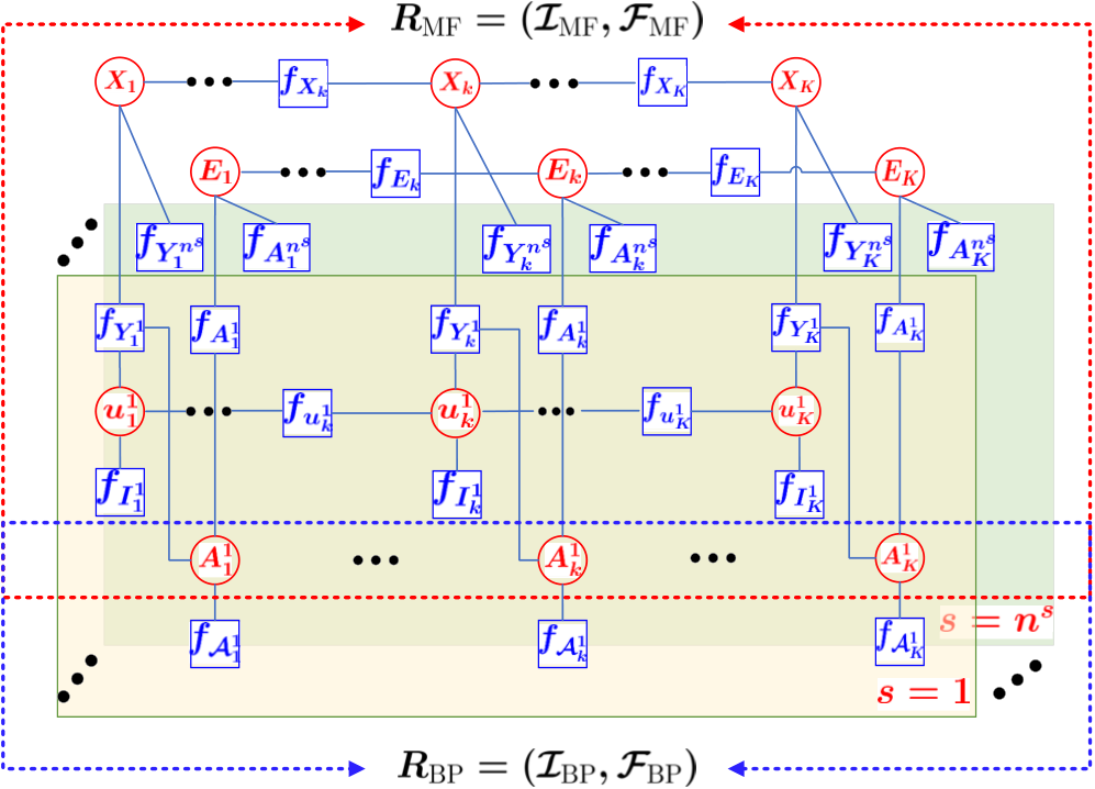
As shown in Fig. 4, the factor factor can be divided into two regions, i.e., MF region and BP region with
| (18) |
It is seen that , , and . According to [16], the joint posterior PDF is expressed as
| (19) |
An approximation of marginal PDFs of each variables in can be derived by minimizing the region-based free energy , which is defined by [17]
| (20) |
where , and the positive functions and , referred as beliefs, are the approximations of and , respectively. The beliefs and have to fulfill the marginalization constraints
| (21) |
and the normalization constraints
| (22) |
Using the Lagrange multipliers method with the constraints given in Eqs. (21) and (22), the combined BP-MF approach [16] yields the belief , i.e., the approximation to the exact marginal probability function , as follows.
| (23) |
with the message update rules given by
| (24) |
where denotes the message sent from variable node to factor node , and denotes the message sent from factor node to variable node . The notation denotes the set of variable nodes except variable node , and denotes a sum over all the variables except . and are positive constants ensuring normalized beliefs. Note that when .
The detailed derivations of each belief with the corresponding subgraphs of the factor graph are presented in the remainder of this section. Note that MP-OTHRs works in a batch processing fashion. For a batch time sequence , different targets may have a different lifetime since target may appear/disapper anytime and anywhere in the region of interests. For ease of exposition (and without loss of generality), we hereafter restrict the notation on the lifetime of all targets from 1 to , and the maximum number of targets during is .
III-B1 Derivation of Belief
By the fact that each target moves independently, the belief of the joint kinematic states of all targets can be factorized as
| (25) |

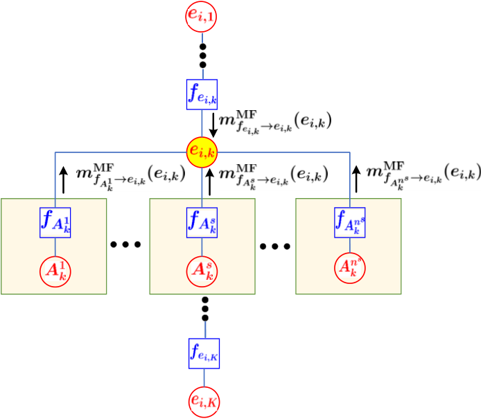
Fig. 5 shows the target kinematic state estimation subgraph of the belief . In Fig. 5, , are the variable nodes to be considered, and our aim is to calculate belief . For each variable node , is the set of all factor nodes connecting to the variable node . Meanwhile, the sets of variable nodes connected to the each factor node in are and , respectively. According to Eq. (23), the belief can be calculated as follows
| (26) |
where the factor-to-variable messages in Eq. (26) can be calculated as follows by using the message update rules given in Eq. (24)
| (27) | ||||
| (28) |
Recall that the variable-to-factor messages , and . Thus,
| (29) |
Substituting Eq. (29) into Eqs. (27), (28), yields
| (30) | ||||
| (31) |
where , and are the expectations of , and taken over corresponding beliefs, respectively. is the state estimation covariance of target at time .
For Gaussian-distributed ionospheric height under a given propagation path , the measurement distribution in Eq. (31) under the nonlinear mapping of a given target state is in general non-Gaussian. In the vein of [4], we use Gaussian approximations, i.e.,
| (32) |
where the covariance is expressed as the sum of two components , including the measurement noise covariance of OTHR and the covariance arising from the uncertain ionospheric height. The latter component is evaluated to a first-order approximation as with being given by Eq. (13), and being the state covariance of the ionospheric height at time .
Substituting Eqs. (30), (31) and (32) into Eq. (26), the belief is rewritten as
| (33) |
where the synthetic measurement and the corresponding covariance are defined as
| (34) |
Since for different OTHR and propagation path , the measurement function and the ionospheric height are different, the synthetic measurements cannot be synthesized further over and . Let
| (35) |
The belief in Eq. (33) can be rewritten as
| (36) |
From Eq. (36), it is seen that is also Gaussian-distributed with its mean and covariance being obtained by a nonlinear filter, such as extended Kalman filter (EKF), that is,
| (37) |
The belief of for a time sequence is derived as
| (38) |
with the mean and the covariance being obtained by a nonlinear fixed-interval smoother, such as Extended Rauch-Tung-Striebel Smoother (ERTSS).
III-B2 Derivation of Belief
Like the target kinematic state, each target appears and disappears independently, the belief of the joint visibility state of targets can be factorized as,
| (39) |
The corresponding subgraph of the target visibility state estimation is shown in Fig. 6, where the to-be-considered variable nodes are . For each variable node , connect it with factor nodes, . The sets of variable nodes connected to each factor node are and , respectively.
According to the message-computation rules given in Eq. (24), the messages from each factor nodes in to the variable node are calculated as
| (40) | ||||
| (41) | ||||
According to Eq. (23), the belief can be computed as
| (42) | ||||
The belief of target visibility state for a time sequence , is derived as
| (43) |
It is seen that the belief follows an HMM with the indirect observation sequence , and the estimation of can be soloved by a forward-backward algorithm [30]. The track management decisions, including track confirmation, maintenance and termination, can be made by comparing the probability of visibility state with different thresholds [31].
Remark 1. The performance of target detection can be improved due to the following reasons. The indirect observation sequence integrates two kinds of information from all paths of all OTHRs, i.e., and , . The target-specific detection probability , which depends on the target visibility state , is used in this paper. Compared with the constant detection probability which is prior information provided by the signal processing module, is posterior information considering the current information on target visibility state, which is benefit to improve the performance of target detection. The association event contains the information that if target is visible or not for propagation path via OTHR , which can be regarded as a prior information provided by measurements.
III-B3 Derivation of Belief
Based on the assumption that the local ionospheric height is radar-specific, the belief of local ionospheric height can be factorized as
| (44) |
and the local ionospheric height subgraph that corresponds to the belief is shown in Fig. 7.

The to-be-considered variable nodes of the local ionospheric height subgraph are . For each variable , connect it with three factor nodes, . The sets of variable nodes connected each factor node are , , and , respectively. According to Eq. (24), the messages from each factor nodes in to the variable node are given as
| (45) | ||||
| (46) | ||||
| (47) |
Noting that the variable-to-factor messages and , we have
| (48) |
Substituting Eq. (48) into Eqs. (45) and (III-B3), yields
| (49) | ||||
| (50) | ||||
| (51) |
where and are the expectation of and taken over corresponding beliefs.
Similar to Eq. (32), the nonlinear measurement function in Eq. (50) is approximated by Gaussian PDF, i.e.,
| (52) |
where , and with being given by Eq. (10).
According to Eq. (23), the belief can be computed by multiplying all the incoming factor-to-variables messages as follows,
where the synthetic measurement is given by Eq. (34) and the corresponding covariance is defined as
| (53) |
From Eq. (III-B3), it is seen that is Gaussian distributed with its mean and covariance being obtained by a nonlinear filter, such as UKF. That is,
| (54) |
The belief of ionospheric heights state for a time sequence , is derived as
| (55) |
In this case, the nonlinear filter in Eq. (54) can be replaced with a nonlinear fixed-interval smoother, such as ERTSS can be exploited. The performance of ionospheric height identification can be improved by combining two kinds of information. One is the direct measurement of ionosondes , and the other is the indirect information from primary OTHR whereas the estimated target kinematic state and its corresponding measurements , are feedback to identify the ionospheric height.
III-B4 Derivation of Belief
We assume that the local multipath data association is independent over different OTHRs and different scans. Accordingly, the belief on multipath data association is factorized as,
| (56) |
Fig. 8 shows the multipath data association subgraph corresponding to the belief , which consists of the variable nodes . There are four factor nodes neighboring to variable node , i.e., where we denote and for simplicity. Note that . The sets of variable nodes connecting to the corresponding factor node are , , and , respectively.

By the message update rules given in Eq. (24), the messages that belong to the MF region () can be calculated as
with . Similar to Eq. (32) and Eq. (52), due to the nonlinear function , the PDF is approximated by Gaussian PDF, i.e.,
| (57) |
where . Thus, the parameter can be calculated as
| (58) |
For the messages belong to the BP region (), we have
| (59) |
Recall that from the frame constraint, for each OTHR , target either produces a measurement through a particular path or is missed. That is, if , then . Eq. (59) can be rewritten as
| (60) |
In a similar way, the message can be rewritten as
| (61) |
According to Eq. (23), the belief can be computed as
| (62) |
III-C Summary
The proposed MP-OTHRs algorithm is summarized as Algorithm 1. To achieve a trade-off between accuracy and latency, MP-OTHRs works in an online fashion using a sliding window.
Compared with MR-MPTF, which is an open-loop, recursive processing and track-level fusion algorithm, MP-OTHRs is a closed-loop, batch processing and measurement-level fusion algorithm. The pros of MP-OTHRs are given as follows: (1) MP-OTHRs adopts the UTM coordinate system to model the target kinematic state, which is more accurate than that of MR-MPTF; (2) MP-OTHRs reduces information loss since it uses the pseudo-measurements to update the global target kinematic state directly; (3) MP-OTHRs implements the estimation of target kinematic state and viability state via smoothers using a batch of measurements, while MR-MPTF adopts a filter; (4) MP-OTHRs is a joint optimization solution, and the information is exchanged among processing modules of latent variables; (5) MP-OTHRs is more computationally effective than MR-MPTF by the fact that MP-OTHRs adopts LBP while MPTF uses the multiple hypothesis strategy to deal with the most time-consuming association problem. As a result, the performance of MP-OTHRs is superior to that of MR-MPTF in the aspects of both target detection and tracking.
III-D Initialization
Initial beliefs , , and the maximum number of potential targets (tracks) are required for MP-OTHRs. We propose a multisensor multipath measurements clustering approach for fast initialization of potential tracks. The initialization procedure for the first sliding window is given as follows.
- •
At time , tentative tracks are established via multisensor multipath measurement clustering, which consists of local track initialization and global track fusion. 1) For each OTHR , we coarsely group the measurements into different subsets with and being the number measurements and number of measurements in the th subset, respectively. To reduce the number of subsets, we assume that the number of measurements satisfies since the maximum number of measurements from the same target is when a target is detected by all propagation paths. In each subset , any two measurements are within a preset threshold vector conditioned on the assumption that they are from the same target via different paths. Each subset with at least two measurements are then utilized to initialize a local tentative track . That is, for each subset , there are total measurement-path association hypothesis, and we transform the measurements in from radar slant coordinate system to UTM coordinate system by traversing all measurement-path association hypothesis, obtaining a set of the transformed path-dependent kinematic states. The path-dependent kinematic state that has the minimum average Mahalanobis distance is then selected and fused to obtain the local kinematic state estimate . The corresponding state covariance is pre-determined based on measurement noise covariance. Set the initial local target visibility probability . 2) The global tracks are obtained by carrying out multisensor track association and fusion. That is, for any pair of local tracks and from different OTHR and , the local tracks of OTHR and of OTHR are possibly from the same target if the Mahalanobis distance is less than the association threshold . To this end, an assignment matrix is constructed by assigning if , otherwise. The corresponding track-to-track association problem with is then solved by S-D assignment techniques [32]. The global target tracks with kinematic states s consist of the fused tracks from those associated local tracks and the unassociated local tracks. Meanwhile, the global initial target visibility state . The initial ionospheric height .
- •
Starting from , for each tentative track , transform the global kinematic state from UTM coordinate system to radar slant coordinate system, and select candidate local multipath measurements individually using gating technique, establish the pseudo-measurement via LBP, and update the kinematic state by a filter. Meanwhile, the visibility probability and ionospheric height are recursively updated by using forward algorithm and Kalman filter, respectively. The measurements that do not fall into the validation gates of any tracks are used to initialize new tracks.
- •
For the batch window , manage tracks based on . Specifically, if the average visibility probability of target larger than the threshold , track is confirmed; or less than the threshold in three successive scans, the track is deleted. is the total number of confirmed potential tracks over the batch window .
IV Simulation and Analysis
IV-A Simulation Scenario
We consider the simulation scenario of multitarget tracking with an OTHR network consisting of two OTHRs. Ten targets move in the overlapping region of the two OTHRs. The detail information of target kinematic state and lifetimes is given in Fig. 9. MP-OTHRs is compared with MR-MPTF. Note that MR-MPTF uses the real value of ionospheric height. We also compare MP-OTHRs with a single OTHR measurement, referred as MP-OTHR1 (only using measurements from OTHR1) and MP-OTHR2 (only using measurements from OTHR2), respectively.
The detailed parameters setting are given as follows: the number of radars ; two ionospheric layers (E-layer and F-layer) and the number of propagation paths ; the number of targets ; the radar receiver parameters and ; the region sizes of range, azimuth and range rate are [1000, 3000] km, [-0.3, 0.3] rad, and [-0.3, 0.3] km/s. For , , the sampling period , the clutter density (the expected clutter number is 21 per scan), the mean ionospheric height km, km, and , , , ; the radar measurement noise covariance , the ionospheric measurement noise covariance . The state transition matrix and , the ionospheric measurement matrix , the process noise covariance and , the initial state covariance . The MP iteration threshold and . The LBP iteration threshold and . Tentative track initialization threshold . Track confirmation threshold . A track is confirmed if the target visibility state and deleted if over three successive scans. The initial target visibility state probability is given by the initialization, and its transition probabilities , . The target visibility state-dependent detection probability and . The window length , the sliding window step is 1, and the gate probability . MR-MPTF implements the single-path target tracking with global nearest neighbour (GNN) tracker, and then carries out the track fusion using multiple hypothesis track fusion (MPTF). GNN uses 3/5 logic to initialize tracks and 3/3 logic to terminate tracks. MPTF keeps first three best hypothesis. The statistical performance comparison of MP-OTHRs and MR-MPTF are given with 100 Monte Carlo runs by varying detection probability.
To evaluate the performance of the four algorithms, it is required to find the association between targets and tracks. We declare that a track is associated to a target if the average difference in both X position and Y position is less than 10 km. Tracks with at least length ten are used to calculate the performance metrics that are given as follows. (1) Number of True Tracks (NTT ): A track is detected as a true one if it is assigned to a target. If more than one track are assigned to the same target, the maximum length track is selected and the rest are ignored. (2) Track Probability of Detection (TPD ): Ratio of the length of a true track to the lifetime of its corresponding target, which indicates the stable tracking capability of an algorithm. (3) Number of False Tracks (NFT ): A track is detected as a false one if it is not assigned to any target. The false tracks consist of the tracks arising from clutter and the multipath tracks that are not assigned to any target. As stated in [7], misleading path association can give rise to multipath tracks that are far away from the true trajectory. (4) Confirmed Track Latency (CTL ): the time delay of the confirmation of a true track. A good target detection capability is achieved by an algorithm if the value of CTL is small. (5) Average Euclidean Error of Target Position (AEEP ): (6) Average Euclidean Error of Target Speed (AEES ). (7) Average Euclidean Error of Ionospheric Height (AEEH ). (8) Mean Optimal Subpattern Assignment (MOSPA ) [33]: (9) Total Execution Time (TET ). For the more detailed definitions of TPD, NFT, AEE, CTL, and TET, refer to [34]. The metrics TPD, CTL, AEEP, AEES, and MOSPA are averaged overall targets, and all of the metrics are averaged over Monte Carlo runs. The notation () indicates the higher (lower) value the metric, the better (worse) the performance is.
IV-B Simulation Results
Fig. 10 shows the multipath detections of ten targets and clutter over all scans when and , , . The trajectories obtained by MP-OTHRs, MP-OTHR1, MP-OTHR2 and MR-MPTF in a single run are shown in Fig. 11. From Fig. 11a, it is seen that MP-OTHRs successfully tracks all ten targets ( - ) but with two false tracks (Trk-15 and Trk-16). Actually, the false tracks Trk-15 and Trk-16 are the multipath tracks of targets and , respectively. The tracking results of MP-OTHRs with a single OTHR are shown in Figs. 11b- 11c. It is seen that MP-OTHR1 successfully tracks nine targets ( - and - ) with one target () being missed, and one false track (Trk-10, the multipath tracks of target ). MP-OTHR2 successfully tracks all ten targets with one false track (Trk-11, the multipath track of target ). Comparing Fig. 11a with the Figs. 11b- 11c, the overall performance of MP-OTHRs is superior to MP-OTHR1 and MP-OTHR2. Fig. 11d shows that MR-MPTF successfully tracks nine targets ( - and - ) with one target being missed, and four (multipath) false tracks (Trk-6, Trk-12, Trk-13, Trk-14). MP-OTHRs is superior to MR-MPTF in the aspects of both target detection and tracking. All the algorithms are implemented in MATLAB R2018a on a PC with an Intel Core i5CPU and 8GB RAM. TET of MP-OTHRs, MP-OTHR1, MP-OTHR2 and MR-MPTF are 14.6 s, 4.21 s, 3.76 s and 77.6 s, respectively.
Fig. 12 shows the performance comparison w. r. t. different detection probability with 100 Monte Carlo runs. As expected, the performance of both target detection and tracking is improved as the increase of detection probability. Specifically, in terms of NVT (shown in Fig. 12a), under the extremely low detection probability , it is hard for a single OTHR, i.e., MP-OTHR1 or MP-OTHR2, to detect valid tracks. Integrating information from the OTHR network, MP-OTHRs and MR-MPTF can track about half of the total targets, and the NVT of MP-OTHRs is greater than that of MR-MPTF. This is because MR-MPTF is based on track-level fusion whereas multipath track is hard to be initialized in slant coordinate system and/or multipath track fusion is unreliable under low detection probability circumstance. MP-OTHRs is based on measurement-level fusion which is more beneficial to track maintenance. As the detection probability increased (e.g., ), NVTs of MP-OTHRs, MP-OTHR1, MP-OTHR2 and MR-MPTF are becoming comparable. This is because the multipath tracks are easy to be detected by MR-MPTF if is high. For a single OTHR, if , the probability of at least one (path) detection for a target is 0.875; the NVTs of MP-OTHR1 and MP-OTHR2 can be improved greatly. In the aspect of NFT (shown in Fig. 12b), which is mainly originated from the multipath tracks, MP-OTHRs performs better than MR-MPTF, especially in the low detection probability cases. With the same reason on NVT, MR-MPTF is easily to produce false tracks. By adopting global track initialization as described in Section III-D, MP-OTHRs does not generate many false tracks. In the aspects of TPD (shown in Fig. 12c) and CLT (shown in Fig. 12d), MP-OTHRs outperforms MP-OTHR1 and MP-OTHR2 in the case of low detection probability since using all the measurements from the OTHR network is benefit to stable target tracking and fast track initialization. TPD of MP-OTHRs and MR-MPTF are comparable, and MP-OTHRs is superior to MR-MPTF on CLT. This is because MR-MPTF adopts the 3/5 logic to confirm tracks while MP-OTHRs uses visibility probability to fast track confirmation. On the tracking error (shown in Figs. 12e-12f), MP-OTHRs has the best tracking accuracy, while MR-MPTF is worst. The reason is that MP-OTHRs adopts the iteration mechanism and state smooth using a batch of measurements; MR-MPTF adopts a filter without iteration and state smooth. Meanwhile, MP-OTHRs is superior to MP-OTHR1 and MP-OTHR2 because of using the measurements from independent OTHRs. As shown in Fig. 12g, the error on ionospheric height is reduced compared with the ionospheric measurement error. This improvement is achieved by the information exchange between local ionospheric height identification and global target state estimation. The improved target track accuracy aids in the identification of ionospheric height. The MSOPA curves (Fig. 12h) show that, on the whole, MP-OTHRs is superior to MR-MPTF. Meanwhile, MP-OTHRs is superior to MP-OTHR1 and MP-OTHR2 in the low detection probability cases.
V Conclusion
We studied target tracking and fusion for an OTHR network. Based on MP, we proposed a joint optimization algorithm for OTHR measurement-level fusion, MP-OTHRs, which is a closed-loop solution among target detection, target tracking, multipath data association and ionospheric height identification. MP-OTHRs improves the performance of target detection and tracking significantly comparing with the track-level fusion method, MR-MPTF. Compared with a single OTHR, MP-OTHRs improves target detection and tracking performance, especially in the low detection probability cases.
VI Acknowledgments
This work was supported in part by the National Natural Science Foundation of China (Grant No. 61873211, 61501378, 61503305, 61790552).
References
- [1] G. Fabrizio, High frequency over-the-horizon radar: fundamental principles, signal processing, and practical applications. McGraw Hill Professional, 2013.
- [2] S. Anderson, “Remote sensing with the Jindalee skywave radar,” IEEE Journal of Oceanic Engineering, vol. 11, no. 2, pp. 158–163, 1986.
- [3] D. J. Percival and K. A. White, “Multihypothesis fusion of multipath over-the-horizon radar tracks,” in Proceedings of SPIE, vol. 3373, 1998, pp. 440–451.
- [4] G. Pulford, “OTHR multipath tracking with uncertain coordinate registration,” IEEE Transactions on Aerospace and Electronic Systems, vol. 40, no. 1, pp. 38–56, 2004.
- [5] G. W. Pulford and R. J. Evans, “A multipath data association tracker for over-the-horizon radar,” IEEE Transactions on Aerospace and Electronic Systems, vol. 34, no. 4, pp. 1165–1183, 1998.
- [6] B. Habtemariam, R. Tharmarasa, T. Thayaparan, M. Mallick, and T. Kirubarajan, “A multiple-detection joint probabilistic data association filter,” IEEE Journal of Selected Topics in Signal Processing, vol. 7, no. 3, pp. 461 – 471, 2013.
- [7] T. Sathyan, T.-J. Chin, S. Arulampalam, and D. Suter, “A multiple hypothesis tracker for multitarget tracking with multiple simultaneous measurements,” IEEE Journal of Selected Topics in Signal Processing, vol. 7, no. 3, pp. 448 – 460, 2013.
- [8] X. Tang, X. Chen, M. McDonald, R. Mahler, R. Tharmarasa, and T. Kirubarajan, “A multiple-detection probability hypothesis density filter,” IEEE Transactions on Signal Processing, vol. 63, no. 8, pp. 2007–2019, 2015.
- [9] J. Chen, H. Ma, C. Liang, and Y. Zhang, “OTHR multipath tracking using the Bernoulli filter,” IEEE Transactions on Aerospace and Electronic Systems, vol. 50, no. 3, pp. 1974–1990, 2014.
- [10] H. Lan, Y. Liang, Q. Pan, F. Yang, and C. Guan, “An EM algorithm for multipath state estimation in OTHR target tracking.” IEEE Transactions on Signal Processing, vol. 62, no. 11, pp. 2814–2826, 2014.
- [11] H. Lan, Y. Liang, Z. Wang, F. Yang, and Q. Pan, “Distributed ECM algorithm for OTHR multipath target tracking with unknown ionospheric heights,” IEEE Journal of Selected Topics in Signal Processing, vol. 12, no. 1, pp. 61–75, 2018.
- [12] M. G. Rutten, N. J. Gordon, and D. J. Percival, “Track fusion in over-the-horizon radar networks,” in Proceedings of the Sixth International Conference on Information Fusion, 2003, pp. 334–341.
- [13] P. W. Sarunic, K. White, and M. G. Rutten, “Over-the-horizon radar multipath and multisensor track fusion algorithm development,” Defence Science and Technology Organisation SAllsbury (AUSTRALIA), Tech. Rep., 2001.
- [14] D. M. Blei, A. Kucukelbir, and J. D. McAuliffe, “Variational inference: A review for statisticians,” Journal of the American Statistical Association, vol. 112, no. 518, pp. 859–877, 2017.
- [15] J. S. Yedidia, W. T. Freeman, and Y. Weiss, “Understanding belief propagation and its generalizations,” Exploring artificial intelligence in the new millennium, vol. 8, pp. 236–239, 2003.
- [16] E. Riegler, G. E. Kirkelund, C. N. Manchón, M.-A. Badiu, and B. H. Fleury, “Merging belief propagation and the mean field approximation: A free energy approach,” IEEE Transactions on Information Theory, vol. 59, no. 1, pp. 588–602, 2012.
- [17] J. S. Yedidia, W. T. Freeman, and Y. Weiss, “Constructing free-energy approximations and generalized belief propagation algorithms,” IEEE Transactions on Information Theory, vol. 51, no. 7, pp. 2282–2312, 2005.
- [18] F. Meyer, T. Kropfreiter, J. L. Williams, R. Lau, F. Hlawatsch, P. Braca, and M. Z. Win, “Message passing algorithms for scalable multitarget tracking,” Proceedings of the IEEE, vol. 106, no. 2, pp. 221–259, 2018.
- [19] R. Turner, S. Bottone, and B. Avasarala, “A complete variational tracker,” in Proceedings of the 27th International Conference on Neural Information Processing Systems-Volume 1, 2014, pp. 496–504.
- [20] H. Lan, S. Sun, Z. Wang, Q. Pan, and Z. Zhang, “Joint target detection and tracking in multipath environment: A variational Bayesian approach,” IEEE Transactions on Aerospace and Electronic Systems, 2019.
- [21] J. L. Williams and R. A. Lau, “Approximate evaluation of marginal association probabilities with belief propagation,” IEEE Transactions on Aerospace and Electronic Systems, vol. 50, no. 4, pp. 2942–2959, 2014.
- [22] ——, “Multiple scan data association by convex variational inference,” IEEE Transactions on Signal Processing, vol. 66, no. 8, pp. 2112–2127, 2016.
- [23] F. Meyer, P. Braca, P. Willett, and F. Hlawatsch, “A scalable algorithm for tracking an unknown number of targets using multiple sensors,” IEEE Transactions on Signal Processing, vol. 65, no. 13, pp. 3478–3493, 2017.
- [24] G. Soldi, F. Meyer, P. Braca, and F. Hlawatsch, “Self-tuning algorithms for multisensor-multitarget tracking using belief propagation,” IEEE Transactions on Signal Processing, vol. 67, no. 15, pp. 3922–3937, 2019.
- [25] Y. Zhang, G. J. Frazer, and M. G. Amin, “Concurrent operation of two over-the-horizon radars,” IEEE Journal of Selected Topics in Signal Processing, vol. 1, no. 1, pp. 114–123, 2007.
- [26] E. Grafarend, “The optimal universal transverse mercator projection,” in Geodetic Theory Today. Springer, 1995, pp. 51–51.
- [27] Y. D. Zhang, A. Ahmed, and B. Himed, “Target altitude estimation in over-the-horizon radar (preprint),” AFRL/RYMD WPAFB United States, Tech. Rep., 2019.
- [28] Y. Bar-Shalom and W. Blair, Multitarget-multisensor Tracking: Applications and Advances.
- [29] R. H. Anderson and J. L. Krolik, “Track association for over-the-horizon radar with a statistical ionospheric model,” IEEE Transactions on Signal Processing, vol. 50, no. 11, pp. 2632–2643, 2002.
- [30] L. R. Rabiner, “A tutorial on hidden Markov models and selected applications in speech recognition,” Proceedings of the IEEE, vol. 77, no. 2, pp. 257–286, 1989.
- [31] N. Li and X. R. Li, “Tracker design based on target perceivability,” IEEE Transactions on Aerospace and Electronic Systems, vol. 37, no. 1, pp. 214–225, 2001.
- [32] Y. Bar-Shalom and X. Li, Multitarget-Multisensor Tracking: Principles and Techniques. YBS Publishing, Storrs, 1995.
- [33] D. Schuhmacher, B.-T. Vo, and B.-N. Vo, “A consistent metric for performance evaluation of multi-object filters,” IEEE Transactions on Signal Processing, vol. 56, no. 8, pp. 3447–3457, 2008.
- [34] A. A. Gorji, R. Tharmarasa, and T. Kirubarajan, “Performance measures for multiple target tracking problems,” in Proceedings of 14th International Conference on Information Fusion, 2011, pp. 1–8.