跳到论文正文
W Papers独立论文阅读器 arXiv:2003.09960 论文正文 计算阅读时间 · 0%
引用这篇论文根据当前论文元数据生成,正式投稿前建议核对。


License: arXiv.org perpetual non-exclusive license
arXiv:2003.09960v3 [stat.ML] 27 Nov 2021

Efficient Clustering for Stretched Mixtures: Landscape and Optimality

Kaizheng Wang Thanks: Department of Industrial Engineering and Operations Research, Columbia University. Email: kaizheng.wang@columbia.edu    Yuling Yan Thanks: Department of Operations Research and Financial Engineering, Princeton University. Email: yulingy@princeton.edu    Mateo Díaz Thanks: Center for Applied Mathematics, Cornell University. Email: md825@cornell.edu
December 2020
Abstract

This paper considers a canonical clustering problem where one receives unlabeled samples drawn from a balanced mixture of two elliptical distributions and aims for a classifier to estimate the labels. Many popular methods including PCA and k-means require individual components of the mixture to be somewhat spherical, and perform poorly when they are stretched. To overcome this issue, we propose a non-convex program seeking for an affine transform to turn the data into a one-dimensional point cloud concentrating around −1-1 and 11, after which clustering becomes easy. Our theoretical contributions are two-fold: (1) we show that the non-convex loss function exhibits desirable geometric properties when the sample size exceeds some constant multiple of the dimension, and (2) we leverage this to prove that an efficient first-order algorithm achieves near-optimal statistical precision without good initialization. We also propose a general methodology for clustering with flexible choices of feature transforms and loss objectives.

Keywords: clustering, dimensionality reduction, unsupervised learning, landscape, nonconvex optimization

1 Introduction

Clustering is a fundamental problem in data science, especially in the early stages of knowledge discovery. Its wide applications include genomics (Eisen et al. 1998; Remm et al. 2001), imaging (Filipovych et al. 2011), linguistics (Di Marco and Navigli 2013), networks (Adamic and Glance 2005), and finance (Arnott 1980; Zhu et al. 2020), to name a few. They have motivated numerous characterizations for “clusters” and associated learning procedures.

In this paper, we consider a binary clustering problem where the data come from a mixture of two elliptical distributions. Suppose that we observe i.i.d. samples {𝑿i}i=1n⊆ℝd\{\bm{X}_{i}\}_{i=1}^{n}\subseteq\mathbb{R}^{d} from the latent variable model

𝑿i=𝝁0+𝝁​Yi+𝚺1/2​𝒁i,i∈[n].\displaystyle\bm{X}_{i}=\bm{\mu}_{0}+\bm{\mu}Y_{i}+\bm{\Sigma}^{1/2}\bm{Z}_{i},\qquad i\in[n]. (1)

Here 𝝁0,𝝁∈ℝd\bm{\mu}_{0},\penalty\ \bm{\mu}\in\mathbb{R}^{d} and 𝚺≻0\bm{\Sigma}\succ 0 are deterministic; Yi∈{±1}Y_{i}\in\{\pm 1\} and 𝒁i∈ℝd\bm{Z}_{i}\in\mathbb{R}^{d} are independent random quantities; ℙ⁡(Yi=−1)=ℙ⁡(Yi=1)=1/2\mathbb{P}(Y_{i}=-1)=\mathbb{P}(Y_{i}=1)=1/2, and 𝒁i\bm{Z}_{i} is an isotropic random vector whose distribution is spherically symmetric with respect to the origin. 𝑿i\bm{X}_{i} is elliptically distributed (Fang et al. 1990) given YiY_{i}. The goal of clustering is to estimate {Yi}i=1n\{Y_{i}\}_{i=1}^{n} from {𝑿i}i=1n\{\bm{X}_{i}\}_{i=1}^{n}. Moreover, it is desirable to build a classifier with straightforward out-of-sample extension that predicts labels for future samples.

As a warm-up example, assume for simplicity that 𝒁i\bm{Z}_{i} has density and 𝝁0=𝟎\bm{\mu}_{0}=\mathbf{0}. The Bayes-optimal classifier is

φ𝜷⋆​(𝒙)=sgn(𝜷⋆⁣⊤​𝒙)={1if ​𝜷⋆⁣⊤​𝒙≥0−1otherwise,\varphi_{\bm{\beta}^{\star}}(\bm{x})=\mathop{\mathrm{sgn}}(\bm{\beta}^{\star\top}\bm{x})=\begin{cases}1&\text{if }\bm{\beta}^{\star\top}\bm{x}\geq 0\\ -1&\text{otherwise}\end{cases},

with any 𝜷⋆∝𝚺−1​𝝁\bm{\beta}^{\star}\propto\bm{\Sigma}^{-1}\bm{\mu}. A natural strategy for clustering is to learn a linear classifier φ𝜷​(𝒙)=sgn(𝜷⊤​𝒙)\varphi_{\bm{\beta}}(\bm{x})=\mathop{\mathrm{sgn}}(\bm{\beta}^{\top}\bm{x}) with discriminative coefficients 𝜷∈ℝd\bm{\beta}\in\mathbb{R}^{d} estimated from the samples. Note that

𝜷⊤​𝑿i=(𝜷⊤​𝝁)​Yi+𝜷⊤​𝚺1/2​𝒁i​=𝑑​(𝜷⊤​𝝁)​Yi+𝜷⊤​𝚺​𝜷​Zi,\displaystyle\bm{\beta}^{\top}\bm{X}_{i}=(\bm{\beta}^{\top}\bm{\mu})Y_{i}+\bm{\beta}^{\top}\bm{\Sigma}^{1/2}\bm{Z}_{i}\overset{d}{=}(\bm{\beta}^{\top}\bm{\mu})Y_{i}+\sqrt{\bm{\beta}^{\top}\bm{\Sigma}\bm{\beta}}Z_{i},

where Zi=𝒆1⊤​𝒁iZ_{i}=\bm{e}_{1}^{\top}\bm{Z}_{i} is the first coordinate of 𝒁i\bm{Z}_{i}. The transformed data {𝜷⊤​𝑿i}i=1n\{\bm{\beta}^{\top}\bm{X}_{i}\}_{i=1}^{n} are noisy observations of scaled labels {(𝜷⊤​𝝁)​Yi}i=1n\{(\bm{\beta}^{\top}\bm{\mu})Y_{i}\}_{i=1}^{n}. A discriminative feature mapping 𝒙↦𝜷⊤​𝒙\bm{x}\mapsto\bm{\beta}^{\top}\bm{x} results in high signal-to-noise ratio (𝜷⊤​𝝁)2/𝜷⊤​𝚺​𝜷(\bm{\beta}^{\top}\bm{\mu})^{2}/\bm{\beta}^{\top}\bm{\Sigma}\bm{\beta}, turning the data into two well-separated clusters in ℝ\mathbb{R}.

When the clusters are almost spherical (𝚺≈𝑰\bm{\Sigma}\approx\bm{I}) or far apart (‖𝝁‖22≫‖𝚺‖2\|\bm{\mu}\|_{2}^{2}\gg\|\bm{\Sigma}\|_{2}), the mean vector 𝝁\bm{\mu} has reasonable discriminative power and the leading eigenvector of the overall covariance matrix 𝝁​𝝁⊤+𝚺\bm{\mu}\bm{\mu}^{\top}+\bm{\Sigma} roughly points that direction. This helps develop and analyze various spectral methods (Vempala and Wang 2004; Ndaoud 2018) based on Principal Component Analysis (PCA). kk-means (Lu and Zhou 2016) and its semidefinite relaxation (Mixon et al. 2017; Royer 2017; Fei and Chen 2018; Giraud and Verzelen 2018; Chen and Yang 2018) are also closely related. As they are built upon the Euclidean distance, a key assumption is the existence of well-separated balls each containing the bulk of one cluster. Existing works typically require ‖𝝁‖22/‖𝚺‖2\|\bm{\mu}\|_{2}^{2}/\|\bm{\Sigma}\|_{2} to be large under models like (1). Yet, the separation is better measured by 𝝁⊤​𝚺−1​𝝁\bm{\mu}^{\top}\bm{\Sigma}^{-1}\bm{\mu}, which always dominates ‖𝝁‖22/‖𝚺‖2\|\bm{\mu}\|_{2}^{2}/\|\bm{\Sigma}\|_{2}. Those methods may fail when the clusters are separated but “stretched”. As a toy example, consider a Gaussian mixture 12​N​(𝝁,𝚺)+12​N​(−𝝁,𝚺)\frac{1}{2}N(\bm{\mu},\bm{\Sigma})+\frac{1}{2}N(-\bm{\mu},\bm{\Sigma}) in ℝ2\mathbb{R}^{2} where 𝝁=(1,0)⊤\bm{\mu}=(1,0)^{\top} and the covariance matrix 𝚺=diag⁡(0.1,10)\bm{\Sigma}={\rm diag}(0.1,10) is diagonal. Then the distribution consists of two separated but stretched ellipses. PCA returns the direction (0,1)⊤(0,1)^{\top} that maximizes the variance but is unable to tell the clusters apart.

To get high discriminative power under general conditions, we search for 𝜷\bm{\beta} that makes {𝜷⊤​𝑿i}i=1n\{\bm{\beta}^{\top}\bm{X}_{i}\}_{i=1}^{n} concentrate around the label set {±1}\{\pm 1\}, through the following optimization problem:

min⁡∑i=1n𝜷∈ℝd⁡f⁡(𝜷⊤​𝑿i).\min_{\bm{\beta}\in\mathbb{R}^{d}}\sum_{i=1}^{n}f(\bm{\beta}^{\top}\bm{X}_{i}). (2)

Here f:ℝ→ℝf:\mathbb{R}\to\mathbb{R} attains its minimum at ±1\pm 1, e.g. f⁡(x)=(x2−1)2f(x)=(x^{2}-1)^{2}. We name this method as “Clustering via Uncoupled REgression”, or CURE for short. Here ff penalizes the discrepancy between predictions {𝜷⊤​𝑿i}i=1n\{\bm{\beta}^{\top}\bm{X}_{i}\}_{i=1}^{n} and labels {Yi}i=1n\{Y_{i}\}_{i=1}^{n}. In the unsupervised setting, we have no access to the one-to-one correspondence but can still enforce proximity on the distribution level, i.e.

1n​∑i=1nδ𝜷⊤​𝑿i≈12​δ−1+12​δ1.\displaystyle\frac{1}{n}\sum_{i=1}^{n}\delta_{\bm{\beta}^{\top}\bm{X}_{i}}\approx\frac{1}{2}\delta_{-1}+\frac{1}{2}\delta_{1}. (3)

A good approximate solution to (2) leads to |𝜷⊤​𝑿i|≈1|\bm{\beta}^{\top}\bm{X}_{i}|\approx 1. That is, the transformed data form two clusters around ±1\pm 1. The symmetry of the mixture distribution automatically ensures balance between the clusters. Thus (2) is an uncoupled regression problem based on (3). Above we focus on the centered case (𝝁0=𝟎)(\bm{\mu}_{0}=\mathbf{0}) merely to illustrate main ideas. Our general methodology

minα∈ℝ,𝜷∈ℝd⁡{1n​∑i=1nf⁡(α+𝜷⊤​𝑿i)+12​(α+𝜷⊤​𝝁^0)2},\displaystyle\min_{\alpha\in\mathbb{R},\penalty\ \bm{\beta}\in\mathbb{R}^{d}}\bigg\{\frac{1}{n}\sum_{i=1}^{n}f(\alpha+\bm{\beta}^{\top}\bm{X}_{i})+\frac{1}{2}(\alpha+\bm{\beta}^{\top}\hat{\bm{\mu}}_{0})^{2}\bigg\}, (4)

where 𝝁^0=1n​∑i=1n𝑿i\hat{\bm{\mu}}_{0}=\frac{1}{n}\sum_{i=1}^{n}\bm{X}_{i}, deals with arbitrary 𝝁0\bm{\mu}_{0} by incorporating an intercept term α\alpha.

Main contributions.

We propose a clustering method through (4) and study it under the model (1) without requiring the clusters to be spherical. Under mild assumptions, we prove that an efficient algorithm achieves near-optimal statistical precision even in the absence of a good initialization.

  • •

    (Loss function design) We construct an appropriate loss function ff by clipping the growth of the quartic function (x2−1)2/4(x^{2}-1)^{2}/4 outside some interval centered at 00. As a result, ff has two “valleys” at ±1\pm 1 and does not grow too fast, which is beneficial to statistical analysis and optimization.

  • •

    (Landscape analysis) We characterize the geometry of the empirical loss function when n/dn/d exceeds some constant. In particular, all second-order stationary points, where the smallest eigenvalues of Hessians are not significantly negative, are nearly optimal in the statistical sense.

  • •

    (Efficient algorithm with near-optimal statistical property) We show that with high probability, a perturbed version of gradient descent algorithm starting from 𝟎\mathbf{0} yields a solution with near-optimal statistical property after O~​(n/d+d2/n)\tilde{O}(n/d+d^{2}/n) iterations (up to polylogarithmic factors).

The formulation (4) is uncoupled linear regression for binary clustering. Beyond that, we introduce a unified framework which learns feature transforms to identify clusters with possibly non-convex shapes. That provides a principled way of designing flexible unsupervised learning algorithms.

We introduce the model and methodology in Section 2, conduct theoretical analysis in Section 3, present numerical results in Section 4, and finally conclude the paper with a discussion in Section 5.

Related work.

Methodologies for clustering can be roughly categorized as generative and discriminative ones. Generative approaches fit mixture models for the joint distribution of features 𝑿\bm{X} and label YY to make predictions (Moitra and Valiant 2010; Kannan et al. 2005; Anandkumar et al. 2014). Their success usually hinges on well-specified models and precise estimation of parameters. Since clustering is based on the conditional distribution of YY given 𝑿\bm{X}, it only involves certain functional of parameters. Generative approaches often have high overhead in terms of sample size and running time. On the other hand, discriminative approaches directly aim for predictive classifiers. A common strategy is to learn a transform to turn the data into a low-dimensional point cloud that facilitates clustering. Statistical analysis of mixture models lead to information-based methods (Bridle et al. 1992; Krause et al. 2010), analogous to the logistic regression for supervised classification. Geometry-based methods uncover latent structures in an intuitive way, similar to the support vector machine. Our method CURE belongs to this family. Other examples include projection pursuit (Friedman and Tukey 1974; Peña and Prieto 2001a), margin maximization (Ben-Hur et al. 2001; Xu et al. 2005), discriminative kk-means (Ye et al. 2008; Bach and Harchaoui 2008), graph cut optimization by spectral methods (Shi and Malik 2000; Ng et al. 2002) and semidefinite programming (Weinberger and Saul 2006), correlation clustering Bunea et al. 2020; Jarrow et al. 2020. Discriminative methods are easily integrated with modern tools such as deep neural networks (Springenberg 2015; Xie et al. 2016). The list above is far from exhaustive.

The formulation (4) is invariant under invertible affine transforms of data and thus tackles stretched mixtures which are catastrophic for many existing approaches. A recent paper Kushnir et al. 2019 uses random projections to tackle such problem but requires the separation between two clusters to grow at the order of d\sqrt{d}, where dd is the dimension. There have been provable algorithms dealing with general models with multiple classes and minimal separation conditions (Brubaker and Vempala 2008; Kalai et al. 2010; Belkin and Sinha 2015). However, their running time and sample complexity are large polynomials in the dimension and desired precision. In the class of two-component mixtures we consider, CURE has near-optimal (linear) sample complexity and runs fast in practice. Another relevant area of study is clustering under sparse mixture models (Azizyan et al. 2015; Verzelen and Arias-Castro 2017), where additional structures help handle non-spherical clusters efficiently.

The vanilla version of CURE in (2) is closely related to the Projection Pursuit (PP) (Friedman and Tukey 1974) and Independent Component Analysis (ICA) (Hyvärinen and Oja 2000). PP and ICA find the most nontrivial direction by maximizing the deviation of the projected data from some null distribution (e.g. Gaussian). Their objective functions are designed using key features of that. Notably, Peña and Prieto 2001a propose clustering algorithms based on extreme projections that maximize and minimize the kurtosis; Verzelen and Arias-Castro 2017 use the first absolute moment and skewness to construct objective functions in pursuit of projections for clustering. On the contrary, CURE stems from uncoupled regression and minimizes the discrepancy between the projected data and some target distribution. This makes it generalizable beyond linear feature transforms with flexible choices of objective functions. Moreover, CURE has nice computational guarantees while only a few algorithms for PP and ICA do. The formulation (2) with double-well loss ff also appears in the real version of Phase Retrieval (PR) (Candes et al. 2015) for recovering a signal 𝜷\bm{\beta} from noisy quadratic measurements Yi≈(𝑿i⊤​𝜷)2Y_{i}\approx(\bm{X}_{i}^{\top}\bm{\beta})^{2}. In both CURE and PR, one observes the magnitudes of labels/outputs without sign information. However, algorithmic study of PR usually require {𝑿i}i=1n\{\bm{X}_{i}\}_{i=1}^{n} to be isotropic Gaussian; most efficient algorithms need good initializations by spectral methods. Those cannot be easily adapted to clustering. Our analysis of CURE could provide a new way of studying PR under more general conditions.

Notation.

Let [n]={1,2,⋯,n}[n]=\{1,2,\cdots,n\}. Denote by |⋅||\cdot| the absolute value of a real number or cardinality of a set. For real numbers aa and bb, let a∧b=min⁡{a,b}a\wedge b=\min\{a,b\} and a∨b=max⁡{a,b}a\vee b=\max\{a,b\}. For nonnegative sequences {an}n=1∞\{a_{n}\}_{n=1}^{\infty} and {bn}n=1∞\{b_{n}\}_{n=1}^{\infty}, we write an≲bna_{n}\lesssim b_{n} or an=O⁡(bn)a_{n}=O(b_{n}) if there exists a positive constant CC such that an≤C​bna_{n}\leq Cb_{n}. In addition, we write an=O~​(bn)a_{n}=\tilde{O}(b_{n}) if an=O⁡(bn)a_{n}=O(b_{n}) holds up to some logarithmic factor; an≍bna_{n}\asymp b_{n} if an≲bna_{n}\lesssim b_{n} and bn≲anb_{n}\lesssim a_{n}. We let 𝟏S\mathbf{1}_{S} be the indicator function of a set SS. We equip ℝd\mathbb{R}^{d} with the inner product ⟨𝒙,𝒚⟩=𝒙⊤​𝒚\langle{\bm{x}},{\bm{y}}\rangle=\bm{x}^{\top}\bm{y}, Euclidean norm ‖𝒙‖2=⟨𝒙,𝒙⟩\|\bm{x}\|_{2}=\sqrt{\langle{\bm{x}},{\bm{x}}\rangle} and canonical bases {𝒆j}j=1d\{\bm{e}_{j}\}_{j=1}^{d}. Let 𝕊d−1={𝒙∈ℝd:‖𝒙‖2=1}\mathbb{S}^{d-1}=\{\bm{x}\in\mathbb{R}^{d}:\penalty\ \|\bm{x}\|_{2}=1\}, B⁡(𝒙,r)={𝒚∈ℝd:‖𝒚−𝒙‖2≤r}B(\bm{x},r)=\{\bm{y}\in\mathbb{R}^{d}:\penalty\ \|\bm{y}-\bm{x}\|_{2}\leq r\}, and dist⁡(𝒙,S)=inf𝒚∈S‖𝒙−𝒚‖2\mathrm{dist}(\bm{x},S)=\inf_{\bm{y}\in S}\|\bm{x}-\bm{y}\|_{2} for S⊆ℝdS\subseteq\mathbb{R}^{d}. For a matrix 𝑨\bm{A}, we define its spectral norm ‖𝑨‖2=sup‖𝒙‖2=1‖𝑨​𝒙‖2\|\bm{A}\|_{2}=\sup_{\|\bm{x}\|_{2}=1}\|\bm{A}\bm{x}\|_{2}. For a symmetric matrix 𝑨\bm{A}, we use λmax​(𝑨)\lambda_{\max}(\bm{A}) and λmin​(𝑨)\lambda_{\min}(\bm{A}) to represent its largest and smallest eigenvalues, respectively. For a positive definite matrix 𝑨≻0\bm{A}\succ 0, let ‖𝒙‖𝑨=𝒙⊤​𝑨​𝒙\|\bm{x}\|_{\bm{A}}=\sqrt{\bm{x}^{\top}\bm{A}\bm{x}}. Denote by δ𝒙\delta_{\bm{x}} the point mass at 𝒙\bm{x}. Define ∥X∥ψ2=supp≥1p−1/2𝔼1/p|X|p\|X\|_{\psi_{2}}=\sup_{p\geq 1}p^{-1/2}\mathbb{E}^{1/p}|X|^{p} for random variable XX and ‖𝑿‖ψ2=sup‖𝒖‖2=1‖⟨𝒖,𝑿⟩‖ψ2\|\bm{X}\|_{\psi_{2}}=\sup_{\|\bm{u}\|_{2}=1}\|\langle{\bm{u}},{\bm{X}}\rangle\|_{\psi_{2}} for random vector 𝑿\bm{X}.

2 Problem setup

2.1 Elliptical mixture model

Model 1.

Let 𝐗∈ℝd\bm{X}\in\mathbb{R}^{d} be a random vector with the decomposition

𝑿=𝝁0+𝝁​Y+𝚺1/2​𝒁.\displaystyle\bm{X}=\bm{\mu}_{0}+\bm{\mu}Y+\bm{\Sigma}^{1/2}\bm{Z}.

Here 𝛍0,𝛍∈ℝd\bm{\mu}_{0},\bm{\mu}\in\mathbb{R}^{d} and 𝚺≻0\bm{\Sigma}\succ 0 are deterministic; Y∈{±1}Y\in\{\pm 1\} and 𝐙∈ℝd\bm{Z}\in\mathbb{R}^{d} are random and independent. Let Z=𝐞1⊤​𝐙Z=\bm{e}_{1}^{\top}\bm{Z}, ρ\rho be the distribution of 𝐗\bm{X} and {𝐗i}i=1n\{\bm{X}_{i}\}_{i=1}^{n} be i.i.d. samples from ρ\rho.

  • •

    (Balanced classes) ℙ⁡(Y=−1)=ℙ⁡(Y=1)=1/2\mathbb{P}(Y=-1)=\mathbb{P}(Y=1)=1/2;

  • •

    (Elliptical sub-Gaussian noise) 𝒁\bm{Z} is sub-Gaussian with ‖𝒁‖ψ2\|\bm{Z}\|_{\psi_{2}} bounded by some constant MM, 𝔼​𝒁=𝟎\mathbb{E}\bm{Z}=\mathbf{0} and 𝔼⁡(𝒁​𝒁⊤)=𝑰d\mathbb{E}(\bm{Z}\bm{Z}^{\top})=\bm{I}_{d}; its distribution is spherically symmetric with respect to 𝟎\mathbf{0};

  • •

    (Leptokurtic distribution) 𝔼​Z4−3>κ0\mathbb{E}Z^{4}-3>\kappa_{0} holds for some constant κ0>0\kappa_{0}>0;

  • •

    (Regularity) ‖𝝁0‖2\|\bm{\mu}_{0}\|_{2}, ‖𝝁‖2\|\bm{\mu}\|_{2}, λmax​(𝚺)\lambda_{\max}(\bm{\Sigma}) and λmin​(𝚺)\lambda_{\min}(\bm{\Sigma}) are bounded away from 0 and ∞\infty by constants.

We aim to build a classifier ℝd→{±1}\mathbb{R}^{d}\to\{\pm 1\} based solely on the samples {𝑿i}i=1n\{\bm{X}_{i}\}_{i=1}^{n} from a mixture of two elliptical distributions. For simplicity, we assume that the two classes are balanced and focus on the well-conditioned case where the signal strength and the noise level are of constant order. This is already general enough to include stretched clusters incapacitating many popular methods including PCA, kk-means and semi-definite relaxations (Brubaker and Vempala 2008). One may wonder whether it is possible to transform the data into what they can handle. While multiplication by 𝚺−1/2\bm{\Sigma}^{-1/2} yields spherical clusters, precise estimation of 𝚺−1/2\bm{\Sigma}^{-1/2} or 𝚺\bm{\Sigma} is no easy task under the mixture model. Dealing with those d×dd\times d matrices causes overhead expenses in computation and storage. The assumption on positive excess kurtosis prevents the loss function from having undesirable degenerate saddle points and facilitates the proof of algorithmic convergence. It rules out distributions whose kurtoses do not exceed that of the normal distribution, and it is not clear whether there exists an easy fix for that. The last assumption in Model 1 makes the loss landscape regular, helps avoid undesirable technicalities, and is commonly adopted in the study of parameter estimation in mixture models. The Bayes optimal classification error is of constant order, and we want to achieve low excess risk.

2.2 Clustering via Uncoupled Regression

Under Model 1, the Bayes optimal classifier for predicting YY given 𝑿\bm{X} is

Y^Bayes​(𝑿)=sgn(αBayes+𝜷Bayes⊤​𝑿),\displaystyle\hat{Y}^{\mathrm{Bayes}}(\bm{X})=\mathop{\mathrm{sgn}}\big(\alpha^{\mathrm{Bayes}}+\bm{\beta}^{\mathrm{Bayes}\top}\bm{X}\big),

where (αBayes,𝜷Bayes)=(−𝝁0⊤​𝚺−1​𝝁,𝚺−1​𝝁)\big(\alpha^{\mathrm{Bayes}},\bm{\beta}^{\mathrm{Bayes}}\big)=(-\bm{\mu}_{0}^{\top}\bm{\Sigma}^{-1}\bm{\mu},\bm{\Sigma}^{-1}\bm{\mu}). On the other hand, it is easily seen that the following (population-level) least squares problem 𝔼​[(α+𝜷⊤​𝑿)−Y]2\mathbb{E}[(\alpha+\bm{\beta}^{\top}\bm{X})-Y]^{2} has a unique solution (αLR,𝜷LR)=(−c​𝝁0⊤​𝚺−1​𝝁,c​𝚺−1​𝝁)(\alpha^{\mathrm{LR}},\bm{\beta}^{\mathrm{LR}})=(-c\bm{\mu}_{0}^{\top}\bm{\Sigma}^{-1}\bm{\mu},c\bm{\Sigma}^{-1}\bm{\mu}) for some c>0c>0. For the supervised classification problem where we observe {(𝑿i,Yi)}i=1n\{(\bm{X}_{i},Y_{i})\}_{i=1}^{n}, the optimal feature transform can be estimated via linear regression

1n​∑i=1n[(α+𝜷⊤​𝑿i)−Yi]2.\displaystyle\frac{1}{n}\sum_{i=1}^{n}[(\alpha+\bm{\beta}^{\top}\bm{X}_{i})-Y_{i}]^{2}. (5)

This is closely related to Fisher’s Linear Discriminant Analysis (Friedman et al. 2001).

In the unsupervised clustering problem, we no longer observe individual labels {Yi}i=1n\{Y_{i}\}_{i=1}^{n} associated with {𝑿i}i=1n\{\bm{X}_{i}\}_{i=1}^{n} but have population statistics of labels, as the classes are balanced. While (5) directly forces α+𝜷⊤​𝑿i≈Yi\alpha+\bm{\beta}^{\top}\bm{X}_{i}\approx Y_{i} thanks to supervision, here we relax such proximity to the population level:

1n​∑i=1nδα+𝜷⊤​𝑿i≈12​δ−1+12​δ1.\displaystyle\frac{1}{n}\sum_{i=1}^{n}\delta_{\alpha+\bm{\beta}^{\top}\bm{X}_{i}}\approx\frac{1}{2}\delta_{-1}+\frac{1}{2}\delta_{1}. (6)

Thus the regression should be conducted in an uncoupled manner using marginal information about 𝑿\bm{X} and YY. We seek for an affine transformation 𝒙↦α+𝜷⊤​𝒙\bm{x}\mapsto\alpha+\bm{\beta}^{\top}\bm{x} to turn the samples {𝑿i}i=1n\{\bm{X}_{i}\}_{i=1}^{n} into two balanced clusters around ±1\pm 1, after which sgn(α+𝜷⊤​𝑿)\mathop{\mathrm{sgn}}(\alpha+\bm{\beta}^{\top}\bm{X}) predicts YY up to a global sign flip. It is also supported by the geometric intuition in Section 1 based on projections of the mixture distribution.

Clustering via Uncoupled REgression (CURE) is formulated as an optimization problem:

minα∈ℝ,𝜷∈ℝd⁡{1n​∑i=1nf⁡(α+𝜷⊤​𝑿i)+12​(α+𝜷⊤​𝝁^0)2},\displaystyle\min_{\alpha\in\mathbb{R},\penalty\ \bm{\beta}\in\mathbb{R}^{d}}\bigg\{\frac{1}{n}\sum_{i=1}^{n}f(\alpha+\bm{\beta}^{\top}\bm{X}_{i})+\frac{1}{2}(\alpha+\bm{\beta}^{\top}\hat{\bm{\mu}}_{0})^{2}\bigg\}, (7)

where 𝝁^0=1n​∑i=1n𝑿i\hat{\bm{\mu}}_{0}=\frac{1}{n}\sum_{i=1}^{n}\bm{X}_{i}. ff attains its minimum at ±1\pm 1. Minimizing 1n​∑i=1nf⁡(α+𝜷⊤​𝑿i)\frac{1}{n}\sum_{i=1}^{n}f(\alpha+\bm{\beta}^{\top}\bm{X}_{i}) makes the transformed data {α+𝜷⊤​𝑿i}i=1n\{\alpha+\bm{\beta}^{\top}\bm{X}_{i}\}_{i=1}^{n} concentrate around {±1}\{\pm 1\}. However, there are always two trivial minimizers (α,𝜷)=(±1,𝟎)(\alpha,\bm{\beta})=(\pm 1,\mathbf{0}), each of which maps the entire dataset to a single point. What we want are two balanced clusters around −1-1 and 11. The centered case (𝝁0=𝟎\bm{\mu}_{0}=\mathbf{0}) discussed in Section 1 does not have such trouble as α\alpha is set to be 00 and the symmetry of the mixture automatically balance the two clusters. For the general case, we introduce a penalty term (α+𝜷⊤​𝝁^0)2/2(\alpha+\bm{\beta}^{\top}\hat{\bm{\mu}}_{0})^{2}/2 in (7) to drive the center of the transformed data towards 00. The idea comes from moment-matching and is similar to that in Flammarion et al. 2017. If 1n​∑i=1nf⁡(α+𝜷⊤​𝑿i)\frac{1}{n}\sum_{i=1}^{n}f(\alpha+\bm{\beta}^{\top}\bm{X}_{i}) is small, then |α+𝜷⊤​𝑿i|≈1|\alpha+\bm{\beta}^{\top}\bm{X}_{i}|\approx 1 and

1n∑i=1nδα+𝜷⊤​𝑿i≈|{i:α+𝜷⊤​𝑿i≥0}|nδ1+|{i:α+𝜷⊤​𝑿i<0}|nδ−1.\displaystyle\frac{1}{n}\sum_{i=1}^{n}\delta_{\alpha+\bm{\beta}^{\top}\bm{X}_{i}}\approx\frac{|\{i:\penalty\ \alpha+\bm{\beta}^{\top}\bm{X}_{i}\geq 0\}|}{n}\delta_{1}+\frac{|\{i:\penalty\ \alpha+\bm{\beta}^{\top}\bm{X}_{i}<0\}|}{n}\delta_{-1}.

Then, in order to get (6), we simply match the expectations on both sides. This gives rise to the quadratic penalty term in (7). The same idea generalizes beyond the balanced case. When the two classes 11 and −1-1 have probabilities pp and (1−p)(1-p), we can match the mean of {α+𝜷⊤​𝑿i}i=1n\{\alpha+\bm{\beta}^{\top}\bm{X}_{i}\}_{i=1}^{n} with that of a new target distribution p​δ1+(1−p)​δ−1p\delta_{1}+(1-p)\delta_{-1}, and change the quadratic penalty to [(α+𝜷⊤​𝝁^0)−(2​p−1)]2[(\alpha+\bm{\beta}^{\top}\hat{\bm{\mu}}_{0})-(2p-1)]^{2}. When pp is unknown, (7) can always be a surrogate as it seeks for two clusters around ±1\pm 1 and uses the quadratic penalty to prevent any of them from being vanishingly small.

The function ff in (7) requires careful design. To facilitate statistical and algorithmic analysis, we want ff to be twice continuously differentiable and grow slowly. That makes the empirical loss smooth and concentrate well around its population counterpart. In addition, the coercivity of ff, i.e. lim|x|→∞f⁡(x)=+∞\lim_{|x|\to\infty}f(x)=+\infty, confines all minimizers within some ball of moderate size. Similar to the construction of Huber loss (Huber 1964), we start from h⁡(x)=(x2−1)2/4h(x)=(x^{2}-1)^{2}/4, keep its two valleys around ±1\pm 1, clip its growth using linear functions and interpolate in between using cubic splines:

f⁡(x)={h⁡(x),|x|≤ah⁡(a)+h′​(a)​(|x|−a)+h′′​(a)2​(|x|−a)2−h′′​(a)6​(b−a)​(|x|−a)3,a<|x|≤bf⁡(b)+[h′​(a)+b−a2​h′′​(a)]​(|x|−b),|x|>b.\displaystyle f(x)=\begin{cases}h(x),&|x|\leq a\\ h(a)+h^{\prime}(a)(|x|-a)+\frac{h^{\prime\prime}(a)}{2}(|x|-a)^{2}-\frac{h^{\prime\prime}(a)}{6(b-a)}(|x|-a)^{3},&a<|x|\leq b\\ f(b)+[h^{\prime}(a)+\frac{b-a}{2}h^{\prime\prime}(a)](|x|-b),&|x|>b\end{cases}. (8)

Here b>a>1b>a>1 are constants to be determined later. ff is clearly not convex, and neither is the loss function in (7). Yet we can find a good approximate solution efficiently by taking advantage of statistical assumptions and recent advancements in non-convex optimization (Jin et al. 2017).

2.3 Generalization

The aforementioned procedure seeks for a one-dimensional embedding of the data that facilitates clustering. It searches for the best affine function such that the transformed data look like a two-point distribution. The idea of uncoupled linear regression can be easily generalized to any suitable target probability distribution ν\nu over a space 𝒴\mathcal{Y}, class of feature transforms ℱ\mathcal{F} from the original space 𝒳\mathcal{X} to 𝒴\mathcal{Y}, discrepancy measure DD that quantifies the difference between the transformed data distribution and ν\nu, and classification rule g:𝒴→[K]g:\penalty\ \mathcal{Y}\to[K]. CURE for Model 1 above uses 𝒳=ℝd\mathcal{X}=\mathbb{R}^{d}, 𝒴=ℝ\mathcal{Y}=\mathbb{R}, ν=12​δ−1+12​δ1\nu=\frac{1}{2}\delta_{-1}+\frac{1}{2}\delta_{1}, ℱ={𝒙↦α+𝜷⊤𝒙:α∈ℝ,𝜷∈ℝd}\mathcal{F}=\{\bm{x}\mapsto\alpha+\bm{\beta}^{\top}\bm{x}:\penalty\ \alpha\in\mathbb{R},\penalty\ \bm{\beta}\in\mathbb{R}^{d}\}, g⁡(y)=sgn(y)g(y)=\mathop{\mathrm{sgn}}(y) and

D⁡(μ,ν)=|𝔼X∼μ​f​(X)−𝔼X∼ν​f​(X)|+12​|𝔼X∼μ​X−𝔼X∼ν​X|2\displaystyle D(\mu,\nu)=|\mathbb{E}_{X\sim\mu}f(X)-\mathbb{E}_{X\sim\nu}f(X)|+\frac{1}{2}|\mathbb{E}_{X\sim\mu}X-\mathbb{E}_{X\sim\nu}X|^{2} (9)

for any probability distribution μ\mu over ℝ\mathbb{R}. Here we briefly show why (9) is true. Fix any f:𝒙↦α+𝜷⊤​𝒙f:\penalty\ \bm{x}\mapsto\alpha+\bm{\beta}^{\top}\bm{x} in ℱ\mathcal{F} and let μ=1n​∑i=1nδα+𝜷⊤​𝑿i\mu=\frac{1}{n}\sum_{i=1}^{n}\delta_{\alpha+\bm{\beta}^{\top}\bm{X}_{i}} be the transformed data distribution. From f⁡(−1)=f⁡(1)=0f(-1)=f(1)=0 and 𝔼X∼ν​X=0\mathbb{E}_{X\sim\nu}X=0 we see

|𝔼X∼μ​f​(X)−𝔼X∼ν​f​(X)|=𝔼X∼μ​f​(X)=1n​∑i=1nf⁡(α+𝜷⊤​𝑿i),\displaystyle|\mathbb{E}_{X\sim\mu}f(X)-\mathbb{E}_{X\sim\nu}f(X)|=\mathbb{E}_{X\sim\mu}f(X)=\frac{1}{n}\sum_{i=1}^{n}f(\alpha+\bm{\beta}^{\top}\bm{X}_{i}),
|𝔼X∼μ​X−𝔼X∼ν​X|2=(1n​∑i=1n(α+𝜷⊤​𝑿i))2=(α+𝜷⊤​𝝁^0),\displaystyle|\mathbb{E}_{X\sim\mu}X-\mathbb{E}_{X\sim\nu}X|^{2}=\bigg(\frac{1}{n}\sum_{i=1}^{n}(\alpha+\bm{\beta}^{\top}\bm{X}_{i})\bigg)^{2}=(\alpha+\bm{\beta}^{\top}\hat{\bm{\mu}}_{0}),
D⁡(μ,ν)=1n​∑i=1nf⁡(α+𝜷⊤​𝑿i)+12​(α+𝜷⊤​𝝁^0).\displaystyle D(\mu,\nu)=\frac{1}{n}\sum_{i=1}^{n}f(\alpha+\bm{\beta}^{\top}\bm{X}_{i})+\frac{1}{2}(\alpha+\bm{\beta}^{\top}\hat{\bm{\mu}}_{0}).

On top of that, we propose a general framework for clustering (also named as CURE) and describe it at a high level of abstraction in Algorithm 1. Here ρ^n=1n​∑i=1nδ𝑿i\hat{\rho}_{n}=\frac{1}{n}\sum_{i=1}^{n}\delta_{\bm{X}_{i}} is the empirical distribution of data and φ#​ρ^n=1n​∑i=1nδφ⁡(𝑿i)\varphi_{\#}\hat{\rho}_{n}=\frac{1}{n}\sum_{i=1}^{n}\delta_{\varphi(\bm{X}_{i})} is the push-forward distribution. The general version of CURE is a flexible framework for clustering based on uncoupled regression (Rigollet and Weed 2019). For instance, we may set 𝒴=ℝK\mathcal{Y}=\mathbb{R}^{K} and ν=1K​∑k=1nδ𝒆k\nu=\frac{1}{K}\sum_{k=1}^{n}\delta_{\bm{e}_{k}} when there are KK clusters; choose ℱ\mathcal{F} to be the family of convolutional neural networks for image clustering; let DD be the Wasserstein distance or some divergence. CURE is easily integrated with other tools, see Section A.2 in the supplementary material.

Input: Data {𝑿i}i=1n\{\bm{X}_{i}\}_{i=1}^{n} in a feature space 𝒳\mathcal{X}, embedding space 𝒴\mathcal{Y}, target distribution ν\nu over 𝒴\mathcal{Y}, discrepancy measure DD, function class ℱ\mathcal{F}, classification rule gg.
Embedding: find an approximation solution φ^\hat{\varphi} to minφ∈ℱ⁡D⁡(φ#​ρ^n,ν)\min_{\varphi\in\mathcal{F}}D(\varphi_{\#}\hat{\rho}_{n},\nu).
Output: Y^i=g⁡[φ^​(𝑿i)]\hat{Y}_{i}=g[\hat{\varphi}(\bm{X}_{i})] for i∈[n]i\in[n].
Algorithm 1 Clustering via Uncoupled REgression (meta-algorithm)

3 Theoretical analysis

3.1 Main results

Initialize 𝜸0=𝟎\bm{\gamma}^{0}=\bm{0}.
For t=0,1,…t=0,1,\ldots do
   If perturbation condition holds:     Perturb 𝜸t←𝜸t+𝝃t\displaystyle\bm{\gamma}^{t}\leftarrow\bm{\gamma}^{t}+\bm{\xi}^{t} with 𝝃t∼𝒰⁡(B⁡(𝟎,r))\bm{\xi}^{t}\sim\mathcal{U}(B(\bm{0},r))
   If termination condition holds:      Return 𝜸t\bm{\gamma}^{t}
   Update 𝜸t+1←𝜸t−η∇L^1(𝜸t)\bm{\gamma}^{t+1}\leftarrow\bm{\gamma}^{t}-\eta\nabla\hat{L}_{1}(\bm{\gamma}^{t}).
Algorithm 2 Perturbed gradient descent

Let L^1​(α,𝜷)\hat{L}_{1}(\alpha,\bm{\beta}) denote the objective function of CURE in (7). Our main result (Theorem 1) shows that with high probability, a perturbed version of gradient descent (Algorithm 2) applied to L^1\hat{L}_{1} returns an approximate minimizer that is nearly optimal in the statistical sense, within a reasonable number of iterations. Here 𝒰⁡(B⁡(𝟎,r))\mathcal{U}(B(\bm{0},r)) refers to the uniform distribution over B⁡(𝟎,r)B(\bm{0},r). We omit technical details of the algorithm and defer them to Appendix B.4, see Algorithm 3 and Theorem 4 therein. For notational simplicity, we write 𝜸=(α,𝜷)∈ℝ×ℝd\bm{\gamma}=(\alpha,\bm{\beta})\in\mathbb{R}\times\mathbb{R}^{d} and 𝜸Bayes=(αBayes,𝜷Bayes)=(−𝝁⊤​𝚺−1​𝝁0,𝚺−1​𝝁)\bm{\gamma}^{\mathrm{Bayes}}=(\alpha^{\mathrm{Bayes}},\bm{\beta}^{\mathrm{Bayes}})=(-\bm{\mu}^{\top}\bm{\Sigma}^{-1}\bm{\mu}_{0},\bm{\Sigma}^{-1}\bm{\mu}). 𝜸Bayes\bm{\gamma}^{\mathrm{Bayes}} defines the Bayes-optimal classifier 𝒙↦sgn(αBayes+𝜷Bayes⊤​𝒙)\bm{x}\mapsto\mathop{\mathrm{sgn}}(\alpha^{\mathrm{Bayes}}+\bm{\beta}^{\mathrm{Bayes}\top}\bm{x}) for Model 1.

Theorem 1 (Main result).

Let 𝛄0,𝛄1,⋯\bm{\gamma}_{0},\bm{\gamma}_{1},\cdots be the iterates of Algorithm 2 starting from 𝟎\mathbf{0}. Under Model 1 there exist constants c,C,C0,C1,C2>0c,C,C_{0},C_{1},C_{2}>0 independent of nn and dd such that if n≥C​dn\geq Cd and b≥2​a≥C0b\geq 2a\geq C_{0}, then with probability at least 1−C1​[(d/n)C2​d+e−C2​n1/3+n−10]1-C_{1}[(d/n)^{C_{2}d}+e^{-C_{2}n^{1/3}}+n^{-10}], Algorithm 2 terminates within O~​(n/d+d2/n)\tilde{O}(n/d+d^{2}/n) iterations and the output 𝛄^\hat{\bm{\gamma}} satisfies

mins=±1⁡‖s​𝜸^−c​𝜸Bayes‖2≲dn​log⁡(nd).\min_{s=\pm 1}\bigl\|s\hat{\bm{\gamma}}-c\bm{\gamma}^{\mathrm{Bayes}}\bigr\|_{2}\lesssim\sqrt{\frac{d}{n}\log\left(\frac{n}{d}\right)}.

Up to a log⁡(n/d)\sqrt{\log(n/d)} factor, this matches the optimal rate of convergence O⁡(d/n)O(\sqrt{d/n}) for the supervised problem with {Yi}i=1n\{Y_{i}\}_{i=1}^{n} observed, which is even easier than the current one. Theorem 1 asserts that we can achieve a near-optimal rate efficiently without good initialization, although the loss function is non-convex. The two terms n/dn/d and d2/nd^{2}/n in the iteration complexity have nice interpretations. When nn is large, we want a small computational error in order to achieve statistical optimality. The term n/dn/d reflects the cost for this. When nn is small, the empirical loss function does not concentrate well and is not smooth enough either. Hence we choose a conservative step-size and pay the corresponding price d2/nd^{2}/n. A byproduct of Theorem 1 is the following corollary which gives a tight bound for the excess risk. Here ‖g‖∞=supx∈ℝ|g⁡(x)|\|g\|_{\infty}=\sup_{x\in\mathbb{R}}|g(x)| for any g:ℝ→ℝg:\penalty\ \mathbb{R}\to\mathbb{R}. The proof is deferred to Appendix I.

Corollary 1 (Misclassification rate).

Consider the settings in Theorem 1 and suppose that Z=𝐞1⊤​𝐙Z=\bm{e}_{1}^{\top}\bm{Z} has density p∈C1​(ℝ)p\in C^{1}(\mathbb{R}) satisfying ‖p‖∞≤C3\|p\|_{\infty}\leq C_{3} and ‖p′‖∞≤C3\|p^{\prime}\|_{\infty}\leq C_{3} for some constant C3>0C_{3}>0. For 𝛄=(α,𝛃)∈ℝ×ℝd\bm{\gamma}=(\alpha,\bm{\beta})\in\mathbb{R}\times\mathbb{R}^{d}, define its misclassification rate (up to a global sign flip) as

ℛ⁡(𝜸)=mins=±1⁡ℙ⁡(s​sgn(α+𝜷⊤​𝑿)≠Y).\displaystyle\mathcal{R}(\bm{\gamma})=\min_{s=\pm 1}\mathbb{P}\left(s\mathop{\mathrm{sgn}}\big(\alpha+\bm{\beta}^{\top}\bm{X}\big)\neq Y\right).

There exists a constant C4C_{4} such that

ℙ⁡(ℛ⁡(𝜸^)≤ℛ⁡(𝜸Bayes)+C4​d​log⁡(n/d)n)≥1−C1​[(d/n)C2​d+e−C2​n1/3+n−10].\mathbb{P}\bigg(\mathcal{R}(\hat{\bm{\gamma}})\leq\mathcal{R}(\bm{\gamma}^{\mathrm{Bayes}})+\frac{C_{4}d\log(n/d)}{n}\bigg)\geq 1-C_{1}[(d/n)^{C_{2}d}+e^{-C_{2}n^{1/3}}+n^{-10}].

3.2 Sketch of proof

The loss function L^1\hat{L}_{1} is non-convex in general. To find an approximate minimizer efficiently without good initialization, we need L^1\hat{L}_{1} to exhibit benign geometric properties that can be exploited by a simple algorithm. Our choice is the perturbed gradient descent algorithm in Jin et al. 2017, see Algorithm 3 in Appendix B.4 for more details. Provided that the function is smooth enough, it provably converges to an approximate second-order stationary point where the norm of gradient is small and the Hessian matrix does not have any significantly negative eigenvalue. Then it boils down to landscape analysis of L^1\hat{L}_{1} with precise characterizations of approximate stationary points. To begin with, define the population version of L^1\hat{L}_{1} as

L1​(α,𝜷)=𝔼𝑿∼ρ​f​(α+𝜷⊤​𝑿)+12​(α+𝜷⊤​𝝁0)2.L_{1}\left(\alpha,\bm{\beta}\right)=\mathbb{E}_{\bm{X}\sim\rho}f(\alpha+\bm{\beta}^{\top}\bm{X})+\frac{1}{2}(\alpha+\bm{\beta}^{\top}\bm{\mu}_{0})^{2}.
Proposition 1.

There exist positive constants c,ε,δ,ηc,\varepsilon,\delta,\eta and a set S⊆ℝ×ℝdS\subseteq\mathbb{R}\times\mathbb{R}^{d} such that

  1. 1.

    The only two local minima of L1L_{1} are ±𝜸⋆\pm\bm{\gamma}^{\star} with 𝜸⋆=−c​𝜸Bayes\bm{\gamma}^{\star}=-c\bm{\gamma}^{\mathrm{Bayes}};

  2. 2.

    All the other first-order critical points (i.e. with zero gradient) are within δ\delta distance to SS;

  3. 3.

    ‖∇L1​(𝜸)‖2≥ε\|\nabla L_{1}(\bm{\gamma})\|_{2}\geq\varepsilon if dist⁡(𝜸,{±𝜸⋆}∪S)≥δ\mathrm{dist}(\bm{\gamma},\{\pm\bm{\gamma}^{\star}\}\cup S)\geq\delta;

  4. 4.

    ∇2L1​(𝜸)⪰η​𝑰\nabla^{2}L_{1}(\bm{\gamma})\succeq\eta\bm{I} if dist⁡(𝜸,{±𝜸⋆})≤δ\mathrm{dist}(\bm{\gamma},\{\pm\bm{\gamma}^{\star}\})\leq\delta, and λmin​[∇2L1​(𝜸)]≤−η\lambda_{\min}[\nabla^{2}L_{1}(\bm{\gamma})]\leq-\eta if dist⁡(𝜸,S)≤δ\mathrm{dist}(\bm{\gamma},S)\leq\delta.

Proposition 1 shows that all of the approximate second-order critical points of L1L_{1} are close to that corresponding to the Bayes-optimal classifier. Then we will prove similar results for the empirical loss L^1\hat{L}_{1} using concentration inequalities, which leads to the following proposition translating approximate second-order stationarity to estimation error.

Proposition 2.

There exists a constant CC such that the followings happen with high probability: for any 𝛄∈ℝ×ℝd\bm{\gamma}\in\mathbb{R}\times\mathbb{R}^{d} satisfying ‖∇L^1​(𝛄)‖2≤ε/2\|\nabla\hat{L}_{1}(\bm{\gamma})\|_{2}\leq\varepsilon/2 and λmin[∇2L^1(𝛄)]>−η/2\lambda_{\min}[\nabla^{2}\hat{L}_{1}(\bm{\gamma})]>-\eta/2,

mins=±1⁡‖s​𝜸−𝜸⋆‖2≤C⁡(‖∇L^1​(𝜸)‖2+dn​log⁡(nd)).\min_{s=\pm 1}\left\|s\bm{\gamma}-\bm{\gamma}^{\star}\right\|_{2}\leq C\bigg(\big\|\nabla\hat{L}_{1}\left(\bm{\gamma}\right)\big\|_{2}+\sqrt{\frac{d}{n}\log\left(\frac{n}{d}\right)}\bigg).

To achieve near-optimal statistical error (up to a log⁡(n/d)\sqrt{\log(n/d)} factor), Proposition 2 asserts that it suffices to find any 𝜸^\hat{\bm{\gamma}} such that ‖∇L^1​(𝜸^)‖2≲d/n\|\nabla\hat{L}_{1}(\hat{\bm{\gamma}})\|_{2}\lesssim\sqrt{d/n} and λn[∇2L^1(𝜸^)]>−η/2\lambda_{n}[\nabla^{2}\hat{L}_{1}(\hat{\bm{\gamma}})]>-\eta/2. Here the perturbed gradient descent algorithm comes into play, and we see the light at the end of the tunnel. It remains to estimate the Lipschitz smoothness of ∇L^1\nabla\hat{L}_{1} and ∇2L^1\nabla^{2}\hat{L}_{1} with respect to the Euclidean norm. Once this is done, we can directly apply the convergence theorem in Jin et al. 2017 for the perturbed gradient descent. A more comprehensive outline of the proof and all the details are deferred to the Appendix.

4 Numerical experiments

Refer to caption
Figure 1: Visualization of the dataset via PCA. The left plot shows the transformed data via PCA. The right polt is a 2-dimensional visualization of the dataset using PCA.
Refer to caption
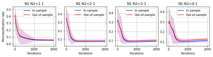
Figure 2: In sample and out-of-sample misclassification rate (with error bar quantifying one standard deviation) vs. iteration count for CURE over 50 independent trials. The four plots corresponds to N2=6000N_{2}=6000, 30003000, 20002000 and 15001500 respectively, while N1N_{1} is always fixed to be 60006000.
Refer to caption
Figure 3: Histograms of transformed out-of-sample data for CURE. The red bins correspond to T-shirts/tops, and the blue bins correspond to pullovers.
Table 1: Misclassification rate of CURE and other methods.
1:11:1 2:12:1 3:13:1 4:14:1
CURE 5.2±0.2%5.2\pm 0.2\% 7.1±0.4%7.1\pm 0.4\% 9.3±0.7%9.3\pm 0.7\% 11.3±1.1%11.3\pm 1.1\%
K-means 45.1%45.1\% 49.7%49.7\% 46.8%46.8\% 45.1%45.1\%
Spectral method (vanilla) 42.2%42.2\% 46.9%46.9\% 49.7%49.7\% 49.0%49.0\%
Spectral method (Gaussian kernel) 49.9%49.9\% 33.4%33.4\% 25.0%25.0\% 20.0%20.0\%

In this section, we conduct numerical experiments on a real dataset. We randomly select N1N_{1} (resp. M1M_{1}) T-shirts/tops and N2N_{2} (resp. M2M_{2}) pullovers from the Fashion-MNIST (Xiao et al. 2017) training (resp. testing) dataset, each of which is a 28×2828\times 28 grayscale image represented by a vector in [0,1]28×28[0,1]^{28\times 28}. The goal is clustering, i.e. learning from those N=N1+N2N=N_{1}+N_{2} unlabeled images to predict the class labels of both NN training samples and M=M1+M2M=M_{1}+M_{2} testing samples. The inputs for CURE and other methods are raw images and their pixel-wise centered versions, respectively. To get a sense why this problem is difficult, we set N1=N2=6000N_{1}=N_{2}=6000 and plot the transformed data via PCA in the left panel of Figure 1: the transformation does not give meaningful clustering information, and the misclassification rate is 42.225%42.225\%. A 2-dimensional visualization of the dataset using PCA (right panel of Figure 1) shows two stretched clusters, which cause the PCA to fail. In this dataset, the bulk of a image corresponds to the belly part of clothing with different grayscales, logos and hence contributes to the most of variability. However, T-shirts and Pullovers are distinguished by sleeves. Hence the two classes can be separated by a linear function that is not related to the leading principle component of data. CURE aims for such direction onto which the projected data exhibit cluster structures.

To show that CURE works beyond our theory, we set N1N_{1} to be 60006000 and choose N2N_{2} from {6000,3000,2000,1500}\{6000,3000,2000,1500\} to include unbalanced cases. We set M1M_{1} to be 10001000 and choose M2M_{2} from {1000,500,333,250}\{1000,500,333,250\}. We use gradient descent with random initialization from the unit sphere and learning rate 10−310^{-3} (instead of perturbed gradient descent) to solve (7) as that requires less tuning. Figure 2 shows the learning curves of CURE over 50 independent trials. Even when the classes are unbalanced, CURE still reliably achieves low misclassification rates. Figure 3 presents histograms of testing data under the feature transform learned by the last (50th) trial of CURE, showing two seperated clusters around ±1\pm 1 corresponding to the two classes. To demonstrate the efficacy of CURE, we compare its misclassification rates with those of K-means and spectral methods on the training sets. We include the standard deviation over 50 independent trials for CURE due to its random initializations; other methods use the default settings (in Python) and thus are regarded as deterministic algorithms. As is shown in Table 1, CURE has the best performance under all settings.

5 Discussion

Motivated by the elliptical mixture model (Model 1), we propose a discriminative clustering method CURE and establish near-optimal statistical guarantees for an efficient algorithm. It is worth pointing out that CURE learns a classification rule that readily predicts labels for any new data. This is an advantage over many existing approaches for clustering and embedding whose out-of-sample extensions are not so straightforward. We impose several technical assumptions (spherical symmetry, constant condition number, positive excess kurtosis, etc.) to simplify the analysis, which we believe can be relaxed. Achieving Bayes optimality in multi-class clustering is indeed very challenging. Under parametric models such as Gaussian mixtures, one may construct suitable loss functions for CURE based on likelihood functions and obtain statistical guarantees. Other directions that are worth exploring include the optimal choice of the target distribution and the discrepancy measure, high-dimensional clustering with additional structures, estimation of the number of clusters, to name a few. We also hope to further extend our methodology and theory to other tasks in unsupervised learning and semi-supervised learning.

The general CURE (Algorithm 1) provides versatile tools for clustering problems. In fact, it is related to several methods in the deep learning literature (Springenberg 2015; Xie et al. 2016; Yang et al. 2017). When we were finishing the paper, we noticed that Genevay et al. 2019 develop a deep clustering algorithm based on kk-means and use optimal transport to incorporate prior knowledge of class proportions. Those methods are built upon certain network architectures (function classes) or loss functions while CURE offers more choices. In addition to the preliminary numerical results, it would be nice to see how CURE tackles more challenging real data problems.

Acknowledgements

We thank Philippe Rigollet and Damek Davis for insightful and stimulating discussions. Kaizheng Wang acknowledges support from the Harold W. Dodds Fellowship at Princeton University where part of the work was done. Yuling Yan is supported in part by the AFOSR grant FA9550-19-1-0030. Mateo Díaz would like to thank his advisor, Damek Davis, for research funding during the completion of this work.

Appendix A Additional numerical experiments

A.1 Two classes

In this section, we provide additional numerical experiments to compare CURE in (7) with other clustering methods on the same real dataset as Section 4. We focus on six methods: (i) discriminative K-means (DisKmeans) in Ye et al. 2008; (ii) a discriminative clustering formulation described in Bach and Harchaoui 2008; Flammarion et al. 2017; (iii) Model-based clustering (Mclust) in Fraley and Raftery 1999; (iv) Projection Pursuit (PP) in Peña and Prieto 2001b; (v) Adaptive LDA-guided K-means Clustering in Ding and Li 2007; and (vi) Minimum Density Hyperplane (MDH) in Pavlidis et al. 2016.

As suggested by Ye et al. 2008, the regularization parameter λ\lambda therein has a significant impact on the performance of DisKmeans. To resolve this issue, they provide an automatic tuning framework. Here we provide a comparison between CURE and DisKmeans. For the DisKmeans, we consider pre-chosen λ∈{0,1,10,100}\lambda\in\{0,1,10,100\} as well as λ\lambda from the automatic tuning procedure suggested by Ye et al. 2008, initialized from 1. Due to high computational cost of DisKmeans with automatic tuning (which includes eigendecomposition of (N1+N2)×(N1+N2)(N_{1}+N_{2})\times(N_{1}+N_{2}) matrix in each iteration), we conduct the experiment on smaller dataset: we fix N1=1000N_{1}=1000 and choose N2N_{2} from {1000,500,333,250}\{1000,500,333,250\}. As is shown in Table 2, CURE has lower misclassification rate under all settings. It is also worth mentioning that the automatic tuning procedure sends λ→∞\lambda\to\infty, in which case DisKmeans is equivalent to classical K-means.

Table 2: Misclassification rate of CURE and disciminative K-means.
1:11:1 2:12:1 3:13:1 4:14:1
CURE / 5.2±0.3%5.2\pm 0.3\% 6.7±0.6%6.7\pm 0.6\% 9.1±0.9%9.1\pm 0.9\% 11.2±1.2%11.2\pm 1.2\%
λ=0\lambda=0 49.9%49.9\% 49.5%49.5\% 49.5%49.5\% 47.7%47.7\%
Discriminative λ=1\lambda=1 48.8%48.8\% 46.6%46.6\% 49.4%49.4\% 48.3%48.3\%
K-means λ=10\lambda=10 46.5%46.5\% 44.2%44.2\% 47.4%47.4\% 41.8%41.8\%
Ye et al. 2008 λ=100\lambda=100 6.6%6.6\% 49.4%49.4\% 46.5%46.5\% 27.2%27.2\%
automatic tuning 43.3%43.3\% 49.4%49.4\% 47.5%47.5\% 45.8%45.8\%

For experiments comparing CURE with other five methods, we still adopt the usual setting of sample size: we fix N1=6000N_{1}=6000 and choose N2N_{2} from {6000,3000,2000,1500}\{6000,3000,2000,1500\}. Model-based clustering (Mclust) in Fraley and Raftery 1999, Projection Pursuit (PP) in Peña and Prieto 2001b and Minimum Density Hyperplane (MDH) in Pavlidis et al. 2016 are implemented using open-source R packages with default settings. In addition:

  1. 1.

    The discriminative clustering method appeared in Bach and Harchaoui 2008; Flammarion et al. 2017 stems from the optimization problem

    min𝒗∈ℝd,𝒚∈{±1}d​‖𝒚−𝑿​𝒗‖22,\underset{\bm{v}\in\mathbb{R}^{d},\bm{y}\in\{\pm 1\}^{d}}{\min}\left\|\bm{y}-\bm{X}\bm{v}\right\|_{2}^{2}, (10)

    where 𝑿\bm{X} is the centered data matrix. We adopt the alternating minimization scheme: given 𝒗\bm{v}, the optimal 𝒚\bm{y} is obtained by sgn(𝑿​𝒗)\mathop{\mathrm{sgn}}(\bm{X}\bm{v}) (or by running K-means on 𝑿​𝒗\bm{X}\bm{v}, which has similar empirical performance) while given 𝒚\bm{y}, the optimal 𝒗\bm{v} is obtained from solving a least squares problem. In the first step, 𝒗\bm{v} is initialized from a uniform distribution over the unit sphere. The iterative algorithm is terminated when 𝒚\bm{y}, the predicted label, no longer changes.

  2. 2.

    Following the instructions in Ding and Li 2007, we implement the adaptive LDA-guided K-means clustering algorithm (Algorithm 1 therein) by alternating between linear discriminant analysis and K-means until convergence.

Table 3 shows the misclassification rate and the standard deviation of CURE and the other five methods over 50 independent trials. It is clear that CURE is more accurate and stable than these five methods under all settings.

Table 3: Misclassification rate of CURE and other methods.
1:11:1 2:12:1 3:13:1 4:14:1
CURE 5.2±0.2%5.2\pm 0.2\% 7.1±0.4%7.1\pm 0.4\% 9.3±0.7%9.3\pm 0.7\% 11.3±1.1%11.3\pm 1.1\%
Method (10) 31.1±13.8%31.1\pm 13.8\% 32.9±13.3%32.9\pm 13.3\% 34.7±12.7%34.7\pm 12.7\% 36.8±11.2%36.8\pm 11.2\%
Mclust 48.7±1.3%48.7\pm 1.3\% 39.1±4.8%39.1\pm 4.8\% 34.1±8.0%34.1\pm 8.0\% 28.2±7.8%28.2\pm 7.8\%
Projection Pursuit 36.9±9.8%36.9\pm 9.8\% 37.4±9.6%37.4\pm 9.6\% 39.7±6.9%39.7\pm 6.9\% 40.6±7.3%40.6\pm 7.3\%
LDA-guided K-means 45.9%45.9\% 49.0%49.0\% 45.6%45.6\% 44.3%44.3\%
MDH 48.6%48.6\% 43.1%43.1\% 38.3%38.3\% 35.2%35.2\%

A.2 Multiple classes

To illustrate how the general CURE in Section 2.3 works, we consider the clustering problem with the first 4 classes in Fashion-MNIST (T-shirt/top, Trouser, Pullover, Dress), each of which has 6000 training samples and 1000 testing samples. Our training process only uses features of training samples and does not touch any labels.

We let the number of classes KK be 4, the embedding space 𝒴\mathcal{Y} be ℝK\mathbb{R}^{K}, the target distribution ν\nu be 1K​∑j=1Kδ𝒆j\frac{1}{K}\sum_{j=1}^{K}\delta_{\bm{e}_{j}}, the discrepancy measure DD be the Wasserstein-1 distance, and define the classification rule g⁡(𝒚)=argminj∈[K]‖𝒚−𝒆j‖2g(\bm{y})=\mathop{\mathrm{argmin}}_{j\in[K]}\|\bm{y}-\bm{e}_{j}\|_{2}. We compare two classes ℱ\mathcal{F} of feature mappings: linear functions and fully-connected neural networks with one hidden layer that has 100 nodes. Initial values All of the weight parameters are initialized using i.i.d. samples from N⁡(0,0.052)N(0,0.05^{2}).

Let f𝜽f_{\bm{\theta}} be a feature transform in ℱ\mathcal{F}, parametrized by 𝜽\bm{\theta}. Denote by {𝒙i}i=1n\{\bm{x}_{i}\}_{i=1}^{n} the samples, where n=4×6000=24000n=4\times 6000=24000. The loss function is

L(𝜽)=W1(1n∑i=1nδf𝜽​(𝒙i),ν)=min𝑷∈[0,1]n×K, 1n⊤​𝑷=𝟏K⊤/K,𝑷​𝟏K=𝟏n/n∑i=1n∑j=1Kpi​j|f𝜽(𝒙i)−𝒆j|.\displaystyle L(\bm{\theta})=W_{1}\bigg(\frac{1}{n}\sum_{i=1}^{n}\delta_{f_{\bm{\theta}}(\bm{x}_{i})},\penalty\ \nu\bigg)=\min_{\bm{P}\in[0,1]^{n\times K},\penalty\ \mathbf{1}_{n}^{\top}\bm{P}=\mathbf{1}_{K}^{\top}/K,\penalty\ \bm{P}\mathbf{1}_{K}=\mathbf{1}_{n}/n}\sum_{i=1}^{n}\sum_{j=1}^{K}p_{ij}|f_{\bm{\theta}}(\bm{x}_{i})-\bm{e}_{j}|.

It is natural to optimize with respect to 𝑷\bm{P} and 𝜽\bm{\theta} in an alternating manner. We apply random sampling techniques to speedup computation. In the tt-th iteration,

  1. 1.

    Draw B=200B=200 samples {𝒙t​i}i=1B\{\bm{x}_{ti}\}_{i=1}^{B} uniform at random (with replacement) from the dataset;

  2. 2.

    Use the Python function ot.sinkhorn2 in library POT (Flamary and Courty 2017) with reg = 0.1 to obtain the solution 𝑷t\bm{P}_{t} to an entropy-regularized version of

    min𝑷∈[0,1]B×K, 1B⊤​𝑷=𝟏K⊤/K,𝑷​𝟏K=𝟏B/B∑i=1B∑j=1Kpi​j|f𝜽t(𝒙t​i)−𝒆j|;\displaystyle\min_{\bm{P}\in[0,1]^{B\times K},\penalty\ \mathbf{1}_{B}^{\top}\bm{P}=\mathbf{1}_{K}^{\top}/K,\penalty\ \bm{P}\mathbf{1}_{K}=\mathbf{1}_{B}/B}\sum_{i=1}^{B}\sum_{j=1}^{K}p_{ij}|f_{\bm{\theta}_{t}}(\bm{x}_{ti})-\bm{e}_{j}|;
  3. 3.

    Update model parameters by 𝜽t+1=𝜽t−η​∂Lt​(𝜽t)\bm{\theta}_{t+1}=\bm{\theta}_{t}-\eta\partial L_{t}(\bm{\theta}_{t}), where ∂\partial is the sub-differential operator, η=10−3\eta=10^{-3} and

    Lt​(𝜽)=∑j=1Kp^i​j​|f𝜽​(𝒙t​i)−𝒆j|,∀𝜽.\displaystyle L_{t}(\bm{\theta})=\sum_{j=1}^{K}\hat{p}_{ij}|f_{\bm{\theta}}(\bm{x}_{ti})-\bm{e}_{j}|,\qquad\forall\bm{\theta}.

An epoch refers to n/B=12n/B=12 consecutive iterations. The learning curves in Figure 4 shows the advantage of neural network and demonstrates the flexibility of CURE with nonlinear function classes.

Refer to caption
Figure 4: 4-class Fashion-MNIST: Testing errors of linear functions and neural networks, with error bar quantifying one standard deviation.

Appendix B Proof sketch of Theorem 1

B.1 Step 1: properties of the test function ff

We now investigate the function ff defined in (8) and relate it to h⁡(x)=(x2−1)2/4h(x)=(x^{2}-1)^{2}/4. As Lemma 1 suggests, |f′||f^{\prime}|, |f′′||f^{\prime\prime}| and |f′′′||f^{\prime\prime\prime}| are all bounded by constants determined by aa and bb; |f′−h′||f^{\prime}-h^{\prime}| and |f′′−h′′||f^{\prime\prime}-h^{\prime\prime}| are bounded by polynomials that are independent of aa and bb. See Appendix D for a proof.

Lemma 1.

When aa is sufficiently large and b≥2​ab\geq 2a, ff has the following properties:

  1. 1.

    f′f^{\prime} is continuous with F1≜supx∈ℝ|f′​(x)|≤2​a2​bF_{1}\triangleq\sup_{x\in\mathbb{R}}|f^{\prime}(x)|\leq 2a^{2}b and |f′(x)−h′(x)|≤7|x|3𝟏{|x|≥a}|f^{\prime}(x)-h^{\prime}(x)|\leq 7|x|^{3}\mathbf{1}_{\{|x|\geq a\}};

  2. 2.

    f′′f^{\prime\prime} is continuous with F2≜supx∈ℝ|f′′​(x)|≤3​a2F_{2}\triangleq\sup_{x\in\mathbb{R}}|f^{\prime\prime}(x)|\leq 3a^{2} and |f′′(x)−h′′(x)|≤9x2𝟏{|x|≥a}|f^{\prime\prime}(x)-h^{\prime\prime}(x)|\leq 9x^{2}\mathbf{1}_{\{|x|\geq a\}};

  3. 3.

    f′′′f^{\prime\prime\prime} exists in ℝ∖{±a,±b}\mathbb{R}\setminus\{\pm a,\pm b\} with F3≜supx∈ℝ∖{±a,±b}|f′′′​(x)|≤6​aF_{3}\triangleq\sup_{x\in\mathbb{R}\setminus\{\pm a,\pm b\}}|f^{\prime\prime\prime}(x)|\leq 6a.

B.2 Step 2: landscape analysis of the population loss

To kick off the landscape analysis we investigate the population version of L^1\hat{L}_{1}, namely

L1​(α,𝜷)=𝔼𝑿∼ρ​f​(α+𝜷⊤​𝑿)+12​(α+𝜷⊤​𝝁0)2.L_{1}\left(\alpha,\bm{\beta}\right)=\mathbb{E}_{\bm{X}\sim\rho}f(\alpha+\bm{\beta}^{\top}\bm{X})+\frac{1}{2}(\alpha+\bm{\beta}^{\top}\bm{\mu}_{0})^{2}. (11)

One of the main obstacles is the complicated piecewise definition of ff, which prevent us from obtaining closed form formulae. We bypass this problem by relating the population loss with ff to that with the quartic function hh. See Appendix E for a proof.

Theorem 2 (Landscape of the population loss).

Consider Model 1 and assume that b≥2​ab\geq 2a. There exist positive constants A,ε,δA,\varepsilon,\delta and η\eta determined by MM, 𝔼​Z4\mathbb{E}Z^{4}, ‖𝛍‖2\|\bm{\mu}\|_{2}, λmax​(𝚺)\lambda_{\max}(\bm{\Sigma}) and λmin​(𝚺)\lambda_{\min}(\bm{\Sigma}) but independent of dd and nn, such that when a>Aa>A,

  1. 1.

    The only two global minima of L1L_{1} are ±𝜸⋆\pm\bm{\gamma}^{\star}, where 𝜸⋆=(−c​𝜷h⊤​𝝁0,c​𝜷h)\bm{\gamma}^{\star}=(-c\bm{\beta}^{h\top}\bm{\mu}_{0},c\bm{\beta}^{h}) for some c∈(1/2,2)c\in(1/2,2) and

    𝜷h=(1+1/‖𝝁‖𝚺−12‖𝝁‖𝚺−14+6​‖𝝁‖𝚺−12+MZ)1/2​𝚺−1​𝝁;\bm{\beta}^{h}=\left(\frac{1+1/\left\|\bm{\mu}\right\|_{\bm{\Sigma}^{-1}}^{2}}{\left\|\bm{\mu}\right\|_{\bm{\Sigma}^{-1}}^{4}+6\left\|\bm{\mu}\right\|_{\bm{\Sigma}^{-1}}^{2}+M_{Z}}\right)^{1/2}\bm{\Sigma}^{-1}\bm{\mu};
  2. 2.

    ‖∇L1​(𝜸)‖2≥ε\|\nabla L_{1}(\bm{\gamma})\|_{2}\geq\varepsilon if dist⁡(𝜸,{±𝜸⋆}∪S)≥δ\mathrm{dist}(\bm{\gamma},\{\pm\bm{\gamma}^{\star}\}\cup S)\geq\delta, where S={𝟎}∪{(−𝜷⊤𝝁0,𝜷):𝝁⊤𝜷=𝟎,𝜷⊤𝚺𝜷=1/MZ}S=\{\mathbf{0}\}\cup\{(-\bm{\beta}^{\top}\bm{\mu}_{0},\bm{\beta}):\penalty\ \bm{\mu}^{\top}\bm{\beta}=\mathbf{0},\penalty\ \bm{\beta}^{\top}\bm{\Sigma}\bm{\beta}=1/M_{Z}\};

  3. 3.

    ∇2L1​(𝜸)⪰η​𝑰\nabla^{2}L_{1}(\bm{\gamma})\succeq\eta\bm{I} if dist⁡(𝜸,{±𝜸⋆})≤δ\mathrm{dist}(\bm{\gamma},\{\pm\bm{\gamma}^{\star}\})\leq\delta, and 𝒖⊤​∇2L1​(𝜸)​𝒖≤−η\bm{u}^{\top}\nabla^{2}L_{1}(\bm{\gamma})\bm{u}\leq-\eta if dist⁡(𝜸,S)≤δ\mathrm{dist}(\bm{\gamma},S)\leq\delta with 𝒖=(0,𝚺−1​𝝁/‖𝚺−1​𝝁‖2)\bm{u}=(0,\bm{\Sigma}^{-1}\bm{\mu}/\|\bm{\Sigma}^{-1}\bm{\mu}\|_{2}).

Theorem 2 precisely characterizes the landscape of L1L_{1}. In particular, all of its critical points make up the set {±𝜸⋆}∪S\{\pm\bm{\gamma}^{\star}\}\cup S, where ±𝜸⋆\pm\bm{\gamma}^{\star} are global minima and SS consists of strict saddles. The local geometry around critical points is also desirable.

B.3 Step 3: landscape analysis of the empirical loss

Based on geometric properties of the population loss L1L_{1}, we establish similar results for the empirical loss L^1\hat{L}_{1} through concentration analysis. See Appendix F for a proof.

Theorem 3 (Landscape of the empirical loss).

Consider Model 1 and assume that b≥2​a≥4b\geq 2a\geq 4. Let 𝛄⋆\bm{\gamma}^{\star} and SS be defined as in Theorem 2. There exist positive constants A,C0,C1,C2,M1,ε,δA,C_{0},C_{1},C_{2},M_{1},\varepsilon,\delta and η\eta determined by MM, MZM_{Z}, ‖𝛍‖2\|\bm{\mu}\|_{2}, λmax​(𝚺)\lambda_{\max}(\bm{\Sigma}) and λmin​(𝚺)\lambda_{\min}(\bm{\Sigma}) but independent of dd and nn, such that when a≥Aa\geq A and n≥C0​dn\geq C_{0}d, the followings hold with probability exceeding 1−C1​(d/n)C2​d−C1​exp⁡(−C2​n1/3)1-C_{1}(d/n)^{C_{2}d}-C_{1}\exp(-C_{2}n^{1/3}):

  1. 1.

    ‖∇L^1​(𝜸)‖2≥ε\|\nabla\hat{L}_{1}(\bm{\gamma})\|_{2}\geq\varepsilon if dist⁡(𝜸,{±𝜸⋆}∪S)≥δ\mathrm{dist}(\bm{\gamma},\{\pm\bm{\gamma}^{\star}\}\cup S)\geq\delta;

  2. 2.

    𝒖⊤​∇2L^1​(𝜸)​𝒖≤−η\bm{u}^{\top}\nabla^{2}\hat{L}_{1}(\bm{\gamma})\bm{u}\leq-\eta if dist⁡(𝜸,S)≤δ\mathrm{dist}(\bm{\gamma},S)\leq\delta, with 𝒖=(0,𝚺−1​𝝁/‖𝚺−1​𝝁‖2)\bm{u}=(0,\bm{\Sigma}^{-1}\bm{\mu}/\|\bm{\Sigma}^{-1}\bm{\mu}\|_{2});

  3. 3.

    ‖∇L^1​(𝜸1)−∇L^1​(𝜸2)‖2≤M1​‖𝜸1−𝜸2‖2\|\nabla\hat{L}_{1}(\bm{\gamma}_{1})-\nabla\hat{L}_{1}(\bm{\gamma}_{2})\|_{2}\leq M_{1}\|\bm{\gamma}_{1}-\bm{\gamma}_{2}\|_{2} and ‖∇2L^1​(𝜸1)−∇2L^1​(𝜸2)‖2≤M1​[1∨(d​log⁡(n/d)/n)]​‖𝜸1−𝜸2‖2\|\nabla^{2}\hat{L}_{1}(\bm{\gamma}_{1})-\nabla^{2}\hat{L}_{1}(\bm{\gamma}_{2})\|_{2}\leq M_{1}[1\vee(d\log(n/d)/\sqrt{n})]\|\bm{\gamma}_{1}-\bm{\gamma}_{2}\|_{2} hold for all 𝜸1,𝜸2∈ℝ×ℝd\bm{\gamma}_{1},\bm{\gamma}_{2}\in\mathbb{R}\times\mathbb{R}^{d}.

Theorem 3 shows that a sample of size n≳dn\gtrsim d suffices for the empirical loss to inherit nice geometric properties from its population counterpart. The corollary below illustrates that as long as we can find an approximate second-order stationary point, then the statistical estimation error can be well controlled by the gradient. We defer the proof of this to Appendix G.

Corollary 2.

Under the settings in Theorem 3, there exist constants C,C1′,C2′C,C_{1}^{\prime},C_{2}^{\prime} such that the followings happen with probability exceeding 1−C1′​(d/n)C2′​d−C1′​exp⁡(−C2′​n1/3)1-C_{1}^{\prime}(d/n)^{C_{2}^{\prime}d}-C_{1}^{\prime}\exp(-C_{2}^{\prime}n^{1/3}): for any 𝛄∈ℝ×ℝd\bm{\gamma}\in\mathbb{R}\times\mathbb{R}^{d} satisfying ‖∇L^1​(𝛄)‖2≤ε\|\nabla\hat{L}_{1}(\bm{\gamma})\|_{2}\leq\varepsilon and λmin​[∇2L^1​(𝛄)]>−η\lambda_{\min}[\nabla^{2}\hat{L}_{1}(\bm{\gamma})]>-\eta,

mins=±1⁡‖s​𝜸−𝜸⋆‖2≤C⁡(‖∇L^1​(𝜸)‖2+dn​log⁡(nd)).\min_{s=\pm 1}\left\|s\bm{\gamma}-\bm{\gamma}^{\star}\right\|_{2}\leq C\bigg(\big\|\nabla\hat{L}_{1}\left(\bm{\gamma}\right)\big\|_{2}+\sqrt{\frac{d}{n}\log\left(\frac{n}{d}\right)}\bigg).

As a result, when the event above happens, any local minimizer 𝛄~\tilde{\bm{\gamma}} of L^1\hat{L}_{1} satisfies

mins=±1⁡‖s​𝜸~−𝜸⋆‖2≤C​dn​log⁡(nd).\min_{s=\pm 1}\left\|s\tilde{\bm{\gamma}}-\bm{\gamma}^{\star}\right\|_{2}\leq C\sqrt{\frac{d}{n}\log\left(\frac{n}{d}\right)}.

B.4 Step 4: convergence guarantees for perturbed gradient descent

The landscape analysis above shows that all local minimizers of L^1\hat{L}_{1} are statistically optimal (up to logarithmic factors), and all saddle points are non-degenerate. Then it boils down to finding any 𝜸\bm{\gamma} whose gradient size is sufficiently small and Hessian has no significantly negative eigenvalue. Thanks to the Lipschitz smoothness of ∇L^1\nabla\hat{L}_{1} and ∇2L^1\nabla^{2}\hat{L}_{1}, this can be efficiently achieved by the perturbed gradient descent algorithm (see Algorithm 3) proposed by Jin et al. 2017. Small perturbation is occasionally added to the iterates, helping escape from saddle points efficiently and thus converge towards local minimizers. Theorem 4 provides algorithmic guarantees for CURE on top of that. We defer the proof to Appendix H.

Implementation of the algorithm requires specification of hyperparameters aa, bb, M1M_{1}, ε\varepsilon and η\eta. Under the regularity assumptions in Model 1, many structural parameters are well-behaved constants and that helps choose hyperparameters at least in a conservative way. In theory, we can let b=2​ab=2a; aa and M1M_{1} be sufficiently large; ε\varepsilon and η\eta be sufficiently small. In our numerical experiments, the algorithm does not appear to be sensitive to choices of hyperparameters. We do not go into much details to avoid distractions.

χ←3​max⁡{log⁡(d​ℓ​Δpgd/(cpgd​εpgd2​δpgd)),4}\chi\leftarrow 3\max\{\log(d\ell\Delta_{\mathrm{pgd}}/(c_{\mathrm{pgd}}\varepsilon_{\mathrm{pgd}}^{2}\delta_{\mathrm{pgd}})),4\}, ηpgd←cpgd/ℓ\eta_{\mathrm{pgd}}\leftarrow c_{\mathrm{pgd}}/\ell, r←cpgd​εpgd/(χ2​ℓ)r\leftarrow\sqrt{c_{\mathrm{pgd}}}\varepsilon_{\mathrm{pgd}}/(\chi^{2}\ell), gthres←cpgd​εpgd/χ2g_{\mathrm{thres}}\leftarrow\sqrt{c_{\mathrm{pgd}}}\varepsilon_{\mathrm{pgd}}/\chi^{2}, fthres←cpgd​εpgd1.5/(χ3​ρ)f_{\mathrm{thres}}\leftarrow c_{\mathrm{pgd}}\varepsilon_{\mathrm{pgd}}^{1.5}/(\chi^{3}\sqrt{\rho}), tthres←χ​ℓ/(cpgd2​ρ​εpgd)t_{\mathrm{thres}}\leftarrow\chi\ell/(c_{\mathrm{pgd}}^{2}\sqrt{\rho\varepsilon_{\mathrm{pgd}}}), tnoise←−tthres−1t_{\mathrm{noise}}\leftarrow-t_{\mathrm{thres}}-1.
Initialize 𝜸0=𝜸pgd\bm{\gamma}^{0}=\bm{\gamma}_{\mathrm{pgd}}.
For t=0,1,…t=0,1,\ldots do
   If ‖∇L^1​(𝜸t)‖2≤gthres\|\nabla\hat{L}_{1}(\bm{\gamma}^{t})\|_{2}\leq g_{\mathrm{thres}} and t−tnoise>tthrest-t_{\mathrm{noise}}>t_{\mathrm{thres}}:
    Update tnoise←tt_{\mathrm{noise}}\leftarrow t,
    Perturb 𝜸t←𝜸t+𝝃t\displaystyle\bm{\gamma}^{t}\leftarrow\bm{\gamma}^{t}+\bm{\xi}^{t} with 𝝃t∼𝒰⁡(B⁡(𝟎,r))\bm{\xi}^{t}\sim\mathcal{U}(B(\bm{0},r))
   If t−tnoise=tthrest-t_{\mathrm{noise}}=t_{\mathrm{thres}} and L^1​(𝜸t)−L^1​(𝜸~tnoise)>−fthres\hat{L}_{1}(\bm{\gamma}^{t})-\hat{L}_{1}(\tilde{\bm{\gamma}}^{t_{\mathrm{noise}}})>-f_{\mathrm{thres}}:
     Return 𝜸~tnoise\tilde{\bm{\gamma}}^{t_{\mathrm{noise}}}
    Update 𝜸t+1←𝜸t−ηpgd∇L^1(𝜸t)\bm{\gamma}^{t+1}\leftarrow\bm{\gamma}^{t}-\eta_{\mathrm{pgd}}\nabla\hat{L}_{1}(\bm{\gamma}^{t}).
Algorithm 3 Perturbed gradient descent PerturbedGD⁡(𝜸pgd,ℓ,ρ,εpgd,cpgd,δpgd,Δpgd)\mathrm{PerturbedGD}(\bm{\gamma}_{\mathrm{pgd}},\ell,\rho,\varepsilon_{\mathrm{pgd}},c_{\mathrm{pgd}},\delta_{\mathrm{pgd}},\Delta_{\mathrm{pgd}})
Theorem 4 (Algorithmic guarantees).

Consider the settings in Theorem 3 and adopt the constants M1M_{1}, ε\varepsilon and η\eta therein. With probability exceeding 1−C1​[(d/n)C2​d+e−C2​n1/3+n−10]1-C_{1}[(d/n)^{C_{2}d}+e^{-C_{2}n^{1/3}}+n^{-10}], Algorithm 3 with parameters 𝛄pgd=𝟎\bm{\gamma}_{\mathrm{pgd}}=\mathbf{0}, ℓ=M1\ell=M_{1}, δpgd=n−11\delta_{\mathrm{pgd}}=n^{-11}, ρ=M1​max⁡{1,d​log⁡(n/d)/n}\rho=M_{1}\max\{1,d\log(n/d)/\sqrt{n}\}, εpgd=min⁡{d​log⁡(n/d)/n,ℓ2/ρ,η2/ρ,ε}\varepsilon_{\mathrm{pgd}}=\min\{\sqrt{d\log(n/d)/n},\ell^{2}/\rho,\eta^{2}/\rho,\varepsilon\} and Δpgd=1/4\Delta_{\mathrm{pgd}}=1/4 terminates within O~​(n/d+d2/n)\tilde{O}({n}/{d}+{d^{2}}/{n}) iterations and the output 𝛄^\hat{\bm{\gamma}} satisfies

‖∇L^1​(𝜸^)‖2≤dn​log⁡(nd)≤εandλmin​(∇2L^1​(𝜸^))≥−η.\bigl\|\nabla\hat{L}_{1}(\hat{\bm{\gamma}})\bigr\|_{2}\leq\sqrt{\frac{d}{n}\log\left(\frac{n}{d}\right)}\leq\varepsilon\qquad\text{and}\qquad\lambda_{\min}\bigl(\nabla^{2}\hat{L}_{1}(\hat{\bm{\gamma}})\bigr)\geq-\eta.

Theorem 4 and Corollary 2 immediately lead to

mins=±1⁡‖s​𝜸^−𝜸⋆‖2≲‖∇L^1​(𝜸^)‖2+dn​log⁡(nd)≲dn​log⁡(nd),\min_{s=\pm 1}\left\|s\hat{\bm{\gamma}}-\bm{\gamma}^{\star}\right\|_{2}\lesssim\big\|\nabla\hat{L}_{1}(\hat{\bm{\gamma}})\big\|_{2}+\sqrt{\frac{d}{n}\log\left(\frac{n}{d}\right)}\lesssim\sqrt{\frac{d}{n}\log\left(\frac{n}{d}\right)},

which finishes the proof of Theorem 1.

Appendix C Preliminaries

Before we start the proof, let us introduce some notations. Recall the definition of the random vector 𝑿=𝝁0+𝝁​Y+𝚺1/2​𝒁\bm{X}=\bm{\mu}_{0}+\bm{\mu}Y+\bm{\Sigma}^{1/2}\bm{Z} and the i.i.d. samples 𝑿1,…,𝑿n∈ℝd\bm{X}_{1},\ldots,\bm{X}_{n}\in\mathbb{R}^{d}. Let 𝑿¯=(1,𝑿)\bar{\bm{X}}=(1,\bm{X}), 𝑿¯i=(1,𝑿i)\bar{\bm{X}}_{i}=(1,\bm{X}_{i}) and 𝝁¯0=(1,𝝁0)\bar{\bm{\mu}}_{0}=(1,\bm{\mu}_{0}). For any 𝜸=(α,𝜷)∈ℝ×ℝd\bm{\gamma}=(\alpha,\bm{\beta})\in\mathbb{R}\times\mathbb{R}^{d}, define

Lλ​(𝜸)=L⁡(𝜸)+λ​R​(𝜸)andL^λ​(𝜸)=L^​(𝜸)+λ​R^​(𝜸),L_{\lambda}(\bm{\gamma})=L(\bm{\gamma})+\lambda R(\bm{\gamma})\qquad\text{and}\qquad\hat{L}_{\lambda}(\bm{\gamma})=\hat{L}(\bm{\gamma})+\lambda\hat{R}(\bm{\gamma}),

where

L⁡(𝜸)=𝔼​f​(𝜸⊤​𝑿¯)=𝔼​f​(α+𝜷⊤​𝑿),L^​(𝜸)=1n​∑i=1nf⁡(𝜸⊤​𝑿¯i)=1n​∑i=1nf⁡(α+𝜷⊤​𝑿i),\displaystyle L(\bm{\gamma})=\mathbb{E}f(\bm{\gamma}^{\top}\bar{\bm{X}})=\mathbb{E}f(\alpha+\bm{\beta}^{\top}\bm{X}),\qquad\hat{L}(\bm{\gamma})=\frac{1}{n}\sum_{i=1}^{n}f(\bm{\gamma}^{\top}\bar{\bm{X}}_{i})=\frac{1}{n}\sum_{i=1}^{n}f(\alpha+\bm{\beta}^{\top}\bm{X}_{i}),
R⁡(𝜸)=12​(α+𝜷⊤​𝝁0)2=12​(𝜸⊤​𝝁¯0)2,R^​(𝜸)=12​(α+𝜷⊤​n−1​∑i=1n𝑿i)2=12​(𝜸⊤​n−1​∑i=1n𝑿¯i)2.\displaystyle R(\bm{\gamma})=\frac{1}{2}(\alpha+\bm{\beta}^{\top}\bm{\mu}_{0})^{2}=\frac{1}{2}(\bm{\gamma}^{\top}\bar{\bm{\mu}}_{0})^{2},\qquad\hat{R}(\bm{\gamma})=\frac{1}{2}(\alpha+\bm{\beta}^{\top}n^{-1}\sum_{i=1}^{n}\bm{X}_{i})^{2}=\frac{1}{2}(\bm{\gamma}^{\top}n^{-1}\sum_{i=1}^{n}\bar{\bm{X}}_{i})^{2}.

Note that the results stated in Section 3 and B focus on the special case when λ=1\lambda=1. The proof in the appendices allows for general choices of λ≥1\lambda\geq 1.

Appendix D Proof of Lemma 1

By direct calculation, one has

f′​(x)={h′​(x),|x|≤a[h′​(a)+h′′​(a)​(|x|−a)−h′′​(a)2​(b−a)​(|x|−a)2]​sgn(x),a<|x|≤b[h′​(a)+b−a2​h′′​(a)]​sgn(x),|x|>b,\displaystyle f^{\prime}(x)=\begin{cases}h^{\prime}(x),&|x|\leq a\\ [h^{\prime}(a)+h^{\prime\prime}(a)(|x|-a)-\frac{h^{\prime\prime}(a)}{2(b-a)}(|x|-a)^{2}]\mathop{\mathrm{sgn}}(x),&a<|x|\leq b\\ [h^{\prime}(a)+\frac{b-a}{2}h^{\prime\prime}(a)]\mathop{\mathrm{sgn}}(x),&|x|>b\end{cases},
f′′​(x)={h′′​(x),|x|≤ah′′​(a)​(1−|x|−ab−a),a<|x|≤b0,|x|>b.,\displaystyle f^{\prime\prime}(x)=\begin{cases}h^{\prime\prime}(x),&|x|\leq a\\ h^{\prime\prime}(a)(1-\frac{|x|-a}{b-a}),&a<|x|\leq b\\ 0,&|x|>b.\end{cases},
f′′′​(x)={h′′′​(x),|x|<a−h′′​(a)b−asgn(x),a<|x|<b0,|x|>b.\displaystyle f^{\prime\prime\prime}(x)=\begin{cases}h^{\prime\prime\prime}(x),&|x|<a\\ -\frac{h^{\prime\prime}(a)}{b-a}\mathop{\mathrm{sgn}}(x),&a<|x|<b\\ 0,&|x|>b\end{cases}.

When aa is sufficiently large and b≥2​ab\geq 2a, we have F1≜supx∈ℝ|f′​(x)|=h′​(a)+b−a2​h′′​(a)≤2​a2​bF_{1}\triangleq\sup_{x\in\mathbb{R}}|f^{\prime}(x)|=h^{\prime}(a)+\frac{b-a}{2}h^{\prime\prime}(a)\leq 2a^{2}b, F2≜supx∈ℝ|f′′​(x)|=h′′​(a)≤3​a2F_{2}\triangleq\sup_{x\in\mathbb{R}}|f^{\prime\prime}(x)|=h^{\prime\prime}(a)\leq 3a^{2}, and F3≜sup|x|≠a,b|f′′′​(x)|=h′′′​(a)∨h′′​(a)b−a≤6​aF_{3}\triangleq\sup_{|x|\neq a,b}|f^{\prime\prime\prime}(x)|=h^{\prime\prime\prime}(a)\vee\frac{h^{\prime\prime}(a)}{b-a}\leq 6a.

In addition, one can also check that when a<|x|≤ba<|x|\leq b, we have |h′​(a)|≤|x|3|h^{\prime}(a)|\leq|x|^{3} and |h′′​(a)|≤3​|x|2|h^{\prime\prime}(a)|\leq 3|x|^{2}, thus

|f′​(x)−h′​(x)|\displaystyle|f^{\prime}(x)-h^{\prime}(x)| ≤|f′​(x)|+|h′​(x)|≤|h′​(a)|+|h′′​(a)​(|x|−a)|+|h′′​(a)​(|x|−a)2/(2​a)|+|x3−x|\displaystyle\leq\left|f^{\prime}(x)\right|+\left|h^{\prime}(x)\right|\leq|h^{\prime}(a)|+|h^{\prime\prime}(a)(|x|-a)|+|h^{\prime\prime}(a)(|x|-a)^{2}/(2a)|+|x^{3}-x|
≤|x|3+3​|x|2+32​|x|2+|x|3≤7​|x|3\displaystyle\leq|x|^{3}+3|x|^{2}+\frac{3}{2}|x|^{2}+|x|^{3}\leq 7|x|^{3}

provided that b≥2​a≥2b\geq 2a\geq 2. When |x|≥b|x|\geq b, we have

|f′​(x)−h′​(x)|\displaystyle|f^{\prime}(x)-h^{\prime}(x)| ≤|f′​(x)|+|h′​(x)|≤|h′​(a)|+|(b−a)​h′′​(a)/2|+|x3−x|\displaystyle\leq\left|f^{\prime}(x)\right|+\left|h^{\prime}(x)\right|\leq|h^{\prime}(a)|+|(b-a)h^{\prime\prime}(a)/2|+|x^{3}-x|
≤|x|3+32​|x|2+|x|3≤4​|x|3.\displaystyle\leq|x|^{3}+\frac{3}{2}|x|^{2}+|x|^{3}\leq 4|x|^{3}.

This combined with f′​(x)=h′​(x)f^{\prime}(x)=h^{\prime}(x) when |x|≤a|x|\leq a gives |f′(x)−h′(x)|≤𝟏{|x|≥a}7|x|3|f^{\prime}(x)-h^{\prime}(x)|\leq\mathbf{1}_{\{|x|\geq a\}}7|x|^{3}. Similarly we have |f′′(x)−h′′(x)|≤𝟏{|x|≥a}9x2|f^{\prime\prime}(x)-h^{\prime\prime}(x)|\leq\mathbf{1}_{\{|x|\geq a\}}9x^{2}.

Appendix E Proof of Theorem 2

It suffices to focus on the special case 𝝁0=𝟎\bm{\mu}_{0}=\bm{0} and 𝚺=𝑰d\bm{\Sigma}=\bm{I}_{d}. We first give a theorem that characterizes the landscape of an auxiliary population loss, which serves as a nice starting point of the study of the actual loss functions that we use.

Theorem 5 (Landscape of the auxillary population loss).

Consider model (1) with 𝛍0=𝟎\bm{\mu}_{0}=\mathbf{0} and 𝚺=𝐈d\bm{\Sigma}=\bm{I}_{d}. Suppose that MZ>3M_{Z}>3. Let h⁡(x)=(x2−1)2/4h(x)=(x^{2}-1)^{2}/4 and λ≥1\lambda\geq 1. The stationary points of the population loss

Lλh​(α,𝜷)=𝔼​h​(α+𝜷⊤​𝑿)+λ2​α2L_{\lambda}^{h}\left(\alpha,\bm{\beta}\right)=\mathbb{E}h\left(\alpha+\bm{\beta}^{\top}\bm{X}\right)+\frac{\lambda}{2}\alpha^{2}

are {(α,𝛃):∇Lλh​(α,𝛃)=𝟎}=S1h∪S2h\{(\alpha,\bm{\beta}):\nabla L_{\lambda}^{h}(\alpha,\bm{\beta})=\bm{0}\}=S_{1}^{h}\cup S_{2}^{h}, where

  1. 1.

    S1h={(0,±𝜷h)}S_{1}^{h}=\{(0,\pm\bm{\beta}^{h})\} consists of global minima, with

    𝜷h=(1+1/‖𝝁‖22‖𝝁‖24+6​‖𝝁‖22+MZ)1/2​𝝁;\bm{\beta}^{h}=\left(\frac{1+1/\left\|\bm{\mu}\right\|_{2}^{2}}{\left\|\bm{\mu}\right\|_{2}^{4}+6\left\|\bm{\mu}\right\|_{2}^{2}+M_{Z}}\right)^{1/2}\bm{\mu};
  2. 2.

    S2h={(0,𝜷):𝝁⊤𝜷=0,∥𝜷∥22=1/MZ}∪{𝟎}S_{2}^{h}=\{(0,\bm{\beta}):\penalty\ \bm{\mu}^{\top}\bm{\beta}=0,\penalty\ \|\bm{\beta}\|_{2}^{2}=1/M_{Z}\}\cup\{\mathbf{0}\} consists of saddle points whose Hessians have negative eigenvalues.

We also have the following quantitative results: there exist positive constants εh,δh\varepsilon^{h},\delta^{h} and ηh\eta^{h} determined by MZM_{Z}, ‖𝛍‖2\|\bm{\mu}\|_{2} and λ\lambda such that

  1. 1.

    ‖∇Lλh​(𝜸)‖2≥εh\|\nabla L^{h}_{\lambda}(\bm{\gamma})\|_{2}\geq\varepsilon^{h} if dist⁡(𝜸,S1h∪S2h)≥δh\mathrm{dist}(\bm{\gamma},S_{1}^{h}\cup S_{2}^{h})\geq\delta^{h};

  2. 2.

    ∇2Lλh​(𝜸)⪰ηh​𝑰\nabla^{2}L_{\lambda}^{h}(\bm{\gamma})\succeq\eta^{h}\bm{I} if dist⁡(𝜸,S1h)≤3​δh\mathrm{dist}(\bm{\gamma},S_{1}^{h})\leq 3\delta^{h}, and 𝒖⊤​∇2Lλh​(𝜸)​𝒖≤−ηh\bm{u}^{\top}\nabla^{2}L_{\lambda}^{h}(\bm{\gamma})\bm{u}\leq-\eta^{h} if dist⁡(𝜸,S2h)≤3​δh\mathrm{dist}(\bm{\gamma},S_{2}^{h})\leq 3\delta^{h} where 𝒖=(0,𝝁/‖𝝁‖2)\bm{u}=(0,\bm{\mu}/\|\bm{\mu}\|_{2}).

Proof.

See Appendix E.1. ∎

The following Lemma 2 controls the difference between the landscape of LλL_{\lambda} and LλhL^{h}_{\lambda} within a compact ball.

Lemma 2.

Let 𝐗\bm{X} be a random vector in ℝd+1\mathbb{R}^{d+1} with ‖𝐗‖ψ2≤M\|\bm{X}\|_{\psi_{2}}\leq M, ff be defined in (8) with b≥2​a≥4b\geq 2a\geq 4, h⁡(x)=(x2−1)2/4h(x)=(x^{2}-1)^{2}/4 for x∈ℝx\in\mathbb{R}, Lλ​(𝛄)=𝔼​f​(𝛄⊤​𝐗)+λ​α2/2L_{\lambda}(\bm{\gamma})=\mathbb{E}f(\bm{\gamma}^{\top}\bm{X})+\lambda\alpha^{2}/2 and Lλh​(𝛄)=𝔼​h​(𝛄⊤​𝐗)+λ​α2/2L_{\lambda}^{h}(\bm{\gamma})=\mathbb{E}h(\bm{\gamma}^{\top}\bm{X})+\lambda\alpha^{2}/2 for 𝛄∈ℝd+1\bm{\gamma}\in\mathbb{R}^{d+1}. There exist constants C1,C2>0C_{1},C_{2}>0 such that for any R>0R>0,

sup‖𝜸‖2≤R‖∇Lλ​(𝜸)−∇Lλh​(𝜸)‖2≤C2​R3​M4​exp⁡(−C1​a2R2​M2),\displaystyle\sup_{\|\bm{\gamma}\|_{2}\leq R}\left\|\nabla L_{\lambda}\left(\bm{\gamma}\right)-\nabla L_{\lambda}^{h}\left(\bm{\gamma}\right)\right\|_{2}\leq C_{2}R^{3}M^{4}\exp\left(-\frac{C_{1}a^{2}}{R^{2}M^{2}}\right),
sup‖𝜸‖2≤R‖∇2Lλ​(𝜸)−∇2Lλh​(𝜸)‖2≤C2​R2​M4​exp⁡(−C1​a2R2​M2).\displaystyle\sup_{\|\bm{\gamma}\|_{2}\leq R}\left\|\nabla^{2}L_{\lambda}\left(\bm{\gamma}\right)-\nabla^{2}L_{\lambda}^{h}\left(\bm{\gamma}\right)\right\|_{2}\leq C_{2}R^{2}M^{4}\exp\left(-\frac{C_{1}a^{2}}{R^{2}M^{2}}\right).

In addition, when 𝔼⁡(𝐗​𝐗⊤)⪰σ2​𝐈\mathbb{E}(\bm{X}\bm{X}^{\top})\succeq\sigma^{2}\bm{I} holds for some σ>0\sigma>0, there exists m>0m>0 determined by MM and σ\sigma such that inf‖𝛄‖2≥3/m‖∇Lλ​(𝛄)‖2≥m\inf_{\|\bm{\gamma}\|_{2}\geq 3/m}\|\nabla L_{\lambda}(\bm{\gamma})\|_{2}\geq m and inf‖𝛄‖2≥3/m‖∇Lλh​(𝛄)‖2≥m\inf_{\|\bm{\gamma}\|_{2}\geq 3/m}\|\nabla L^{h}_{\lambda}(\bm{\gamma})\|_{2}\geq m.

Proof.

See Appendix E.2. ∎

On the one hand, Lemma 2 implies that inf‖𝜸‖2≥3/m‖∇Lλ​(𝜸)‖2≥m\inf_{\|\bm{\gamma}\|_{2}\geq 3/m}\|\nabla L_{\lambda}(\bm{\gamma})\|_{2}\geq m for some constant m>0m>0. Suppose that

εh<m\displaystyle\varepsilon^{h}<m (12)

and define r=3/εhr=3/\varepsilon^{h}. Then

‖∇L1​(𝜸)‖2>εhif‖𝜸‖2≥r.\displaystyle\|\nabla L_{1}(\bm{\gamma})\|_{2}>\varepsilon^{h}\qquad\text{if}\qquad\|\bm{\gamma}\|_{2}\geq r. (13)

Moreover, we can take aa to be sufficiently large such that

sup‖𝜸‖2≤r‖∇L1​(𝜸)−∇L1h​(𝜸)‖2≤εh/2.\displaystyle\sup_{\|\bm{\gamma}\|_{2}\leq r}\big\|\nabla L_{1}\left(\bm{\gamma}\right)-\nabla L_{1}^{h}\left(\bm{\gamma}\right)\big\|_{2}\leq\varepsilon^{h}/2. (14)

On the other hand, from Theorem 5 we know that

‖∇Lλh​(𝜸)‖2≥εhifdist⁡(𝜸,S1h∪S2h)≥δh.\displaystyle\|\nabla L^{h}_{\lambda}(\bm{\gamma})\|_{2}\geq\varepsilon^{h}\qquad\text{if}\qquad\mathrm{dist}(\bm{\gamma},S_{1}^{h}\cup S_{2}^{h})\geq\delta^{h}. (15)

Taking (13), (14) and (15) collectively gives

‖∇Lλ​(𝜸)‖2≥εh/2ifdist⁡(𝜸,S1h∪S2h)≥δh.\displaystyle\|\nabla L_{\lambda}(\bm{\gamma})\|_{2}\geq\varepsilon^{h}/2\qquad\text{if}\qquad\mathrm{dist}(\bm{\gamma},S_{1}^{h}\cup S_{2}^{h})\geq\delta^{h}. (16)

Hence {𝜸:∇Lλ​(𝜸)=𝟎}⊆{𝜸:dist⁡(𝜸,S1h∪S2h)≤δh}\{\bm{\gamma}:\penalty\ \nabla L_{\lambda}(\bm{\gamma})=\bm{0}\}\subseteq\{\bm{\gamma}:\penalty\ \mathrm{dist}(\bm{\gamma},S_{1}^{h}\cup S_{2}^{h})\leq\delta^{h}\} and it yields a decomposition {𝜸:∇Lλ​(𝜸)=𝟎}=S1∪S2\{\bm{\gamma}:\penalty\ \nabla L_{\lambda}(\bm{\gamma})=\bm{0}\}=S_{1}\cup S_{2}, where

Sj⊆{𝜸:dist(𝜸,Sjh)≤δh},∀j=1, 2.\displaystyle S_{j}\subseteq\{\bm{\gamma}:\penalty\ \mathrm{dist}(\bm{\gamma},S_{j}^{h})\leq\delta^{h}\},\qquad\forall j=1,\penalty\ 2. (17)

Consequently, for j=1,2j=1,2 we have

{𝜸:dist⁡(𝜸,Sj)≤2​δh}⊆{𝜸:dist⁡(𝜸,Sjh)≤3​δh}⊆{𝜸:‖𝜸‖2≤3​δh+max𝜸′∈S1h∪S2h⁡‖𝜸′‖2}.\displaystyle\{\bm{\gamma}:\penalty\ \mathrm{dist}(\bm{\gamma},S_{j})\leq 2\delta^{h}\}\subseteq\{\bm{\gamma}:\penalty\ \mathrm{dist}(\bm{\gamma},S_{j}^{h})\leq 3\delta^{h}\}\subseteq\{\bm{\gamma}:\penalty\ \|\bm{\gamma}\|_{2}\leq 3\delta^{h}+\max_{\bm{\gamma}^{\prime}\in S_{1}^{h}\cup S_{2}^{h}}\|\bm{\gamma}^{\prime}\|_{2}\}. (18)

Now we work on the first proposition in Theorem 2 by characterizing S1S_{1}.

Lemma 3.

Consider the model in (1) with 𝛍0=𝟎\bm{\mu}_{0}=\mathbf{0} and 𝚺=𝐈d\bm{\Sigma}=\bm{I}_{d}. Suppose that f∈C2​(ℝ)f\in C^{2}(\mathbb{R}) is even, limx→+∞x​f′​(x)=+∞\lim_{x\to+\infty}xf^{\prime}(x)=+\infty and f′′​(0)<0f^{\prime\prime}(0)<0. Define

Lλ​(α,𝜷)=𝔼​f​(α+𝜷⊤​𝑿)+λ2​α2,∀α∈ℝ,𝜷∈ℝd.\displaystyle L_{\lambda}(\alpha,\bm{\beta})=\mathbb{E}f(\alpha+\bm{\beta}^{\top}\bm{X})+\frac{\lambda}{2}\alpha^{2},\qquad\forall\alpha\in\mathbb{R},\penalty\ \penalty\ \bm{\beta}\in\mathbb{R}^{d}.
  1. 1.

    There exists some c>0c>0 determined by ‖𝝁‖2\|\bm{\mu}\|_{2}, the function ff, and the distribution of ZZ, such that (0,±c​𝝁)(0,\pm c\bm{\mu}) are critical points of LλL_{\lambda};

  2. 2.

    In addition, if f′′f^{\prime\prime} is piecewise differentible and |f′′′​(x)|≤F3<∞|f^{\prime\prime\prime}(x)|\leq F_{3}<\infty almost everywhere, we can find c0>0c_{0}>0 determined by ‖𝝁‖2\|\bm{\mu}\|_{2}, f′′​(0)f^{\prime\prime}(0), F3F_{3} and MM such that c>c0c>c_{0}.

Proof.

See Appendix E.3. ∎

Lemma 3 asserts the existence of two critical points ±𝜸⋆=(0,±c​𝜷h)\pm\bm{\gamma}^{\star}=(0,\pm c\bm{\beta}^{h}) of L1L_{1}, for some cc bounded from below by a constant c0>0c_{0}>0. If

δh<c0​‖𝜷h‖2/4,\displaystyle\delta^{h}<c_{0}\|\bm{\beta}^{h}\|_{2}/4, (19)

then the property of S2hS_{2}^{h} forces

dist⁡(±𝜸⋆,S2h)≥‖𝜸⋆‖2=c​‖𝜷h‖2≥c0​‖𝜷h‖2>4​δh>3​δh.\displaystyle\mathrm{dist}(\pm\bm{\gamma}^{\star},S_{2}^{h})\geq\|\bm{\gamma}^{\star}\|_{2}=c\|\bm{\beta}^{h}\|_{2}\geq c_{0}\|\bm{\beta}^{h}\|_{2}>4\delta^{h}>3\delta^{h}. (20)

It is easily seen from (18) with j=2j=2 that dist⁡(±𝜸⋆,S2)>2​δh\mathrm{dist}(\pm\bm{\gamma}^{\star},S_{2})>2\delta^{h} and ±𝜸⋆∉S2\pm\bm{\gamma}^{\star}\notin S_{2}. Then {𝜸:∇L1​(𝜸)=𝟎}=S1∪S2\{\bm{\gamma}:\penalty\ \nabla L_{1}(\bm{\gamma})=\mathbf{0}\}=S_{1}\cup S_{2} forces

{𝜸⋆,−𝜸⋆}⊆S1.\displaystyle\{\bm{\gamma}^{\star},-\bm{\gamma}^{\star}\}\subseteq S_{1}. (21)

Let us investigate the curvature near S1S_{1}. Lemma 2 and (18) with j=1j=1 allow us to take aa to be sufficiently large such that

supdist⁡(𝜸,S1)≤2​δh‖∇2Lλ​(𝜸)−∇2Lλh​(𝜸)‖2≤ηh/2.\displaystyle\sup_{\mathrm{dist}(\bm{\gamma},S_{1})\leq 2\delta^{h}}\big\|\nabla^{2}L_{\lambda}\left(\bm{\gamma}\right)-\nabla^{2}L_{\lambda}^{h}\left(\bm{\gamma}\right)\big\|_{2}\leq\eta^{h}/2. (22)

Theorem 5 asserts that ∇2Lλh​(𝜸)⪰ηh​𝑰\nabla^{2}L^{h}_{\lambda}(\bm{\gamma})\succeq\eta^{h}\bm{I} if dist⁡(𝜸,S1h)≤3​δh\mathrm{dist}(\bm{\gamma},S_{1}^{h})\leq 3\delta^{h}. By this, (18) with j=1j=1 and (22),

∇2Lλ​(𝜸)⪰(ηh/2)​𝑰ifdist⁡(𝜸,S1)≤2​δh.\displaystyle\nabla^{2}L_{\lambda}(\bm{\gamma})\succeq(\eta^{h}/2)\bm{I}\qquad\text{if}\qquad\mathrm{dist}(\bm{\gamma},S_{1})\leq 2\delta^{h}. (23)

Hence L1L_{1} is strongly convex in {𝜸:dist⁡(𝜸,S1)≤2​δh}\{\bm{\gamma}:\penalty\ \mathrm{dist}(\bm{\gamma},S_{1})\leq 2\delta^{h}\}. Combined with (21), it leads to S1={±𝜸⋆}S_{1}=\{\pm\bm{\gamma}^{\star}\}, and both points therein are local minima.

Let 𝜸h=(0,𝜷h)\bm{\gamma}^{h}=(0,\bm{\beta}^{h}). The fact S1h={±𝜸h}S_{1}^{h}=\{\pm\bm{\gamma}^{h}\} and (17) yields

|c−1|⋅‖𝜷h‖2=‖𝜸⋆−𝜸h‖2=dist⁡(𝜸⋆,S1h)≤δh.\displaystyle|c-1|\cdot\|\bm{\beta}^{h}\|_{2}=\|\bm{\gamma}^{\star}-\bm{\gamma}^{h}\|_{2}=\mathrm{dist}(\bm{\gamma}^{\star},S_{1}^{h})\leq\delta^{h}. (24)

When

δh<‖𝜷h‖2/2,\displaystyle\delta^{h}<\|\bm{\beta}^{h}\|_{2}/2, (25)

we have 1/2<c<3/21/2<c<3/2 as claimed. The global optimality of ±𝜸⋆\pm\bm{\gamma}^{\star} is obvious. Without loss of generality, in Theorem 5 we can always take δh<‖𝜷h‖2​min⁡{c0/3,1/2}\delta^{h}<\|\bm{\beta}^{h}\|_{2}\min\{c_{0}/3,1/2\} and then find εh<m\varepsilon^{h}<m. In that case, (12), (19) and (25) imply the first proposition in Theorem 2.

Next, we study the second proposition in Theorem 2. Let S=S2hS=S_{2}^{h}. Given S1={±𝜸h}S_{1}=\{\pm\bm{\gamma}^{h}\} and S1={±𝜸⋆}S_{1}=\{\pm\bm{\gamma}^{\star}\}, from (24) we know that dist⁡(𝜸,{±𝜸⋆}∪S)≥2​δh\mathrm{dist}(\bm{\gamma},\{\pm\bm{\gamma}^{\star}\}\cup S)\geq 2\delta^{h} implies dist⁡(𝜸,S1h∪S2h)≥2​δh\mathrm{dist}(\bm{\gamma},S_{1}^{h}\cup S_{2}^{h})\geq 2\delta^{h}. This combined with (16) immediately gives

‖∇Lλ​(𝜸)‖2≥εh/2ifdist⁡(𝜸,{±𝜸⋆}∪S)≥2​δh.\displaystyle\|\nabla L_{\lambda}(\bm{\gamma})\|_{2}\geq\varepsilon^{h}/2\qquad\text{if}\qquad\mathrm{dist}(\bm{\gamma},\{\pm\bm{\gamma}^{\star}\}\cup S)\geq 2\delta^{h}.

Hence the second proposition in Theorem 2 holds if

ε=εh/2andδ=2​δh.\displaystyle\varepsilon=\varepsilon^{h}/2\qquad\text{and}\qquad\delta=2\delta^{h}. (26)

Finally, we study the third proposition in Theorem 2. By (23), the first part of that proposition holds when

η=ηh/2andδ=2​δh.\displaystyle\eta=\eta^{h}/2\qquad\text{and}\qquad\delta=2\delta^{h}. (27)

It remains to prove the second part. Lemma 2 and (18) with j=2j=2 allow us to take aa to be sufficiently large such that

supdist⁡(𝜸,S)≤3​δh‖∇2Lλ​(𝜸)−∇2Lλh​(𝜸)‖2≤ηh/2.\displaystyle\sup_{\mathrm{dist}(\bm{\gamma},S)\leq 3\delta^{h}}\big\|\nabla^{2}L_{\lambda}\left(\bm{\gamma}\right)-\nabla^{2}L_{\lambda}^{h}\left(\bm{\gamma}\right)\big\|_{2}\leq\eta^{h}/2. (28)

Theorem 5 asserts that 𝒖⊤​∇2Lλh​(𝜸)​𝒖≤−ηh\bm{u}^{\top}\nabla^{2}L^{h}_{\lambda}(\bm{\gamma})\bm{u}\leq-\eta^{h} for 𝒖=(0,𝝁/‖𝝁‖2)\bm{u}=(0,\bm{\mu}/\|\bm{\mu}\|_{2}) if dist⁡(𝜸,S)≤3​δh\mathrm{dist}(\bm{\gamma},S)\leq 3\delta^{h}. By this, (18) with j=2j=2 and (28),

∇2Lλ(𝜸)≤−ηh/2ifdist(𝜸,S)≤3δh.\displaystyle\nabla^{2}L_{\lambda}(\bm{\gamma})\leq-\eta^{h}/2\qquad\text{if}\qquad\mathrm{dist}(\bm{\gamma},S)\leq 3\delta^{h}. (29)

Hence (26) suffice for the second part of the third proposition to hold.

According to (26) and (27), Theorem 2 holds with ε=εh/2\varepsilon=\varepsilon^{h}/2, δ=2​δh\delta=2\delta^{h} and η=ηh/2\eta=\eta^{h}/2.

E.1 Proof of Theorem 5

E.1.1 Part 1: Characterization of stationary points

Note that

∇Lλh​(α,𝜷)\displaystyle\nabla L_{\lambda}^{h}(\alpha,\bm{\beta}) =𝔼⁡[(1𝑿)​h′​(α+𝜷⊤​𝑿)]+(λ𝟎)\displaystyle=\mathbb{E}\left[\begin{pmatrix}1\\ \bm{X}\end{pmatrix}h^{\prime}(\alpha+\bm{\beta}^{\top}\bm{X})\right]+\begin{pmatrix}\lambda\\ \mathbf{0}\end{pmatrix}
=(𝔼​h′​(α+𝜷⊤​𝑿)+λ𝟎)+(0𝔼⁡[Y​h′​(α+𝜷⊤​𝑿)]​𝝁)+(0𝔼⁡[𝒁​h′​(α+𝜷⊤​𝑿)]).\displaystyle=\begin{pmatrix}\mathbb{E}h^{\prime}(\alpha+\bm{\beta}^{\top}\bm{X})+\lambda\\ \mathbf{0}\end{pmatrix}+\begin{pmatrix}0\\ \mathbb{E}[Yh^{\prime}(\alpha+\bm{\beta}^{\top}\bm{X})]\bm{\mu}\end{pmatrix}+\begin{pmatrix}0\\ \mathbb{E}[\bm{Z}h^{\prime}(\alpha+\bm{\beta}^{\top}\bm{X})]\end{pmatrix}.

Now we will expand individual expected values in this sum. For the first term,

𝔼​h′​(α+𝜷⊤​𝑿)\displaystyle\mathbb{E}h^{\prime}(\alpha+\bm{\beta}^{\top}\bm{X}) =𝔼​(α+𝜷⊤​𝝁​Y+𝜷⊤​𝒁)3−𝔼⁡(α+𝜷⊤​𝝁​Y+𝜷⊤​𝒁)\displaystyle=\mathbb{E}(\alpha+\bm{\beta}^{\top}\bm{\mu}Y+\bm{\beta}^{\top}\bm{Z})^{3}-\mathbb{E}(\alpha+\bm{\beta}^{\top}\bm{\mu}Y+\bm{\beta}^{\top}\bm{Z})
=α3+3​α​𝔼​(𝜷⊤​𝝁​Y)2+3​α​𝔼​(𝜷⊤​𝒁)2+𝔼​(𝜷⊤​𝝁​Y+𝜷⊤​𝒁)3−α\displaystyle=\alpha^{3}+3\alpha\mathbb{E}(\bm{\beta}^{\top}\bm{\mu}Y)^{2}+3\alpha\mathbb{E}(\bm{\beta}^{\top}\bm{Z})^{2}+\mathbb{E}(\bm{\beta}^{\top}\bm{\mu}Y+\bm{\beta}^{\top}\bm{Z})^{3}-\alpha
=α⁡[α2+3​(𝜷⊤​𝝁)2+3​‖𝜷‖22−1],\displaystyle=\alpha[\alpha^{2}+3(\bm{\beta}^{\top}\bm{\mu})^{2}+3\|\bm{\beta}\|_{2}^{2}-1],

where the first line follows since h′​(x)=x3−xh^{\prime}(x)=x^{3}-x, the other two follows from 𝔼⁡(𝒁​𝒁⊤)=𝑰\mathbb{E}(\bm{Z}\bm{Z}^{\top})=\bm{I} plus the fact that YY and 𝒁\bm{Z} are independent, with zero odd moments due to their symmetry.

Using similar arguments,

𝔼⁡[Y​h′​(α+𝜷⊤​𝑿)]\displaystyle\mathbb{E}[Yh^{\prime}(\alpha+\bm{\beta}^{\top}\bm{X})] =𝔼⁡[Y​(α+𝜷⊤​𝝁​Y+𝜷⊤​𝒁)3]−𝔼⁡[Y⁡(α+𝜷⊤​𝝁​Y+𝜷⊤​𝒁)]\displaystyle=\mathbb{E}[Y(\alpha+\bm{\beta}^{\top}\bm{\mu}Y+\bm{\beta}^{\top}\bm{Z})^{3}]-\mathbb{E}[Y(\alpha+\bm{\beta}^{\top}\bm{\mu}Y+\bm{\beta}^{\top}\bm{Z})]
=3​α2​𝔼​[Y⁡(𝜷⊤​𝝁​Y+𝜷⊤​𝒁)]+𝔼⁡[Y​(𝜷⊤​𝝁​Y+𝜷⊤​𝒁)3]−𝜷⊤​𝝁\displaystyle=3\alpha^{2}\mathbb{E}\left[Y(\bm{\beta}^{\top}\bm{\mu}Y+\bm{\beta}^{\top}\bm{Z})\right]+\mathbb{E}[Y(\bm{\beta}^{\top}\bm{\mu}Y+\bm{\beta}^{\top}\bm{Z})^{3}]-\bm{\beta}^{\top}\bm{\mu}
=3​α2​𝜷⊤​𝝁+𝔼⁡[Y​(𝜷⊤​𝝁​Y)3]+3​𝔼​[Y⁡(𝜷⊤​𝝁​Y)]​𝔼​[(𝜷⊤​𝒁)2]−𝜷⊤​𝝁\displaystyle=3\alpha^{2}\bm{\beta}^{\top}\bm{\mu}+\mathbb{E}[Y(\bm{\beta}^{\top}\bm{\mu}Y)^{3}]+3\mathbb{E}[Y(\bm{\beta}^{\top}\bm{\mu}Y)]\mathbb{E}[(\bm{\beta}^{\top}\bm{Z})^{2}]-\bm{\beta}^{\top}\bm{\mu}
=[3​α2+(𝜷⊤​𝝁)2​𝔼​Y4+3​‖𝜷‖22−1]​𝜷⊤​𝝁.\displaystyle=\left[3\alpha^{2}+(\bm{\beta}^{\top}\bm{\mu})^{2}\mathbb{E}Y^{4}+3\|\bm{\beta}\|_{2}^{2}-1\right]\bm{\beta}^{\top}\bm{\mu}.

To work on 𝔼⁡[𝒁​h′​(α+𝜷⊤​𝑿)]=𝔼⁡[𝒁​h′​(α+𝜷⊤​𝝁​Y+𝜷⊤​𝒁)]\mathbb{E}[\bm{Z}h^{\prime}(\alpha+\bm{\beta}^{\top}\bm{X})]=\mathbb{E}[\bm{Z}h^{\prime}(\alpha+\bm{\beta}^{\top}\bm{\mu}Y+\bm{\beta}^{\top}\bm{Z})], we define 𝜷¯=𝜷/‖𝜷‖2\bar{\bm{\beta}}=\bm{\beta}/\|\bm{\beta}\|_{2} for 𝜷≠𝟎\bm{\beta}\neq\mathbf{0} and 𝜷¯=𝟎\bar{\bm{\beta}}=\mathbf{0} otherwise. Observe that (Y,𝜷¯​𝜷¯⊤​𝒁,(𝑰−𝜷¯​𝜷¯⊤)​𝒁)(Y,\bar{\bm{\beta}}\bar{\bm{\beta}}^{\top}\bm{Z},(\bm{I}-\bar{\bm{\beta}}\bar{\bm{\beta}}^{\top})\bm{Z}) and (Y,𝜷¯​𝜷¯⊤​𝒁,−(𝑰−𝜷¯​𝜷¯⊤)​𝒁)(Y,\bar{\bm{\beta}}\bar{\bm{\beta}}^{\top}\bm{Z},-(\bm{I}-\bar{\bm{\beta}}\bar{\bm{\beta}}^{\top})\bm{Z}) have exactly the same joint distribution. As a result,

𝔼⁡[(𝑰−𝜷¯​𝜷¯⊤)​𝒁​h′​(α+𝜷⊤​𝑿)]=𝔼⁡[(𝑰−𝜷¯​𝜷¯⊤)​𝒁​h′​(α+𝜷⊤​𝝁​Y+𝜷⊤​𝒁)]=𝟎.\displaystyle\mathbb{E}[(\bm{I}-\bar{\bm{\beta}}\bar{\bm{\beta}}^{\top})\bm{Z}h^{\prime}(\alpha+\bm{\beta}^{\top}\bm{X})]=\mathbb{E}[(\bm{I}-\bar{\bm{\beta}}\bar{\bm{\beta}}^{\top})\bm{Z}h^{\prime}(\alpha+\bm{\beta}^{\top}\bm{\mu}Y+\bm{\beta}^{\top}\bm{Z})]=\mathbf{0}.

Hence,

𝔼⁡[𝒁​h′​(𝜷⊤​𝑿)]\displaystyle\mathbb{E}[\bm{Z}h^{\prime}(\bm{\beta}^{\top}\bm{X})] =𝔼⁡[𝜷¯​𝜷¯⊤​𝒁​h′​(α+𝜷⊤​𝑿)]=𝔼⁡[𝜷¯⊤​𝒁​h′​(α+𝜷⊤​𝝁​Y+𝜷⊤​𝒁)]​𝜷¯\displaystyle=\mathbb{E}[\bar{\bm{\beta}}\bar{\bm{\beta}}^{\top}\bm{Z}h^{\prime}(\alpha+\bm{\beta}^{\top}\bm{X})]=\mathbb{E}[\bar{\bm{\beta}}^{\top}\bm{Z}h^{\prime}(\alpha+\bm{\beta}^{\top}\bm{\mu}Y+\bm{\beta}^{\top}\bm{Z})]\bar{\bm{\beta}}
=​𝔼​[𝜷¯⊤​𝒁​(α+𝜷⊤​𝝁​Y+𝜷⊤​𝒁)3]​𝜷¯−𝔼⁡[𝜷¯⊤​𝒁​(α+𝜷⊤​𝝁​Y+𝜷⊤​𝒁)]​𝜷¯\displaystyle\overset{}{=}\mathbb{E}[\bar{\bm{\beta}}^{\top}\bm{Z}(\alpha+\bm{\beta}^{\top}\bm{\mu}Y+\bm{\beta}^{\top}\bm{Z})^{3}]\bar{\bm{\beta}}-\mathbb{E}[\bar{\bm{\beta}}^{\top}\bm{Z}(\alpha+\bm{\beta}^{\top}\bm{\mu}Y+\bm{\beta}^{\top}\bm{Z})]\bar{\bm{\beta}}
=3​α2​𝔼​[𝜷¯⊤​𝒁​(𝜷⊤​𝝁​Y+𝜷⊤​𝒁)]​𝜷¯+𝔼⁡[𝜷¯⊤​𝒁​(𝜷⊤​𝝁​Y+𝜷⊤​𝒁)3]​𝜷¯−𝜷\displaystyle=3\alpha^{2}\mathbb{E}[\bar{\bm{\beta}}^{\top}\bm{Z}(\bm{\beta}^{\top}\bm{\mu}Y+\bm{\beta}^{\top}\bm{Z})]\bar{\bm{\beta}}+\mathbb{E}[\bar{\bm{\beta}}^{\top}\bm{Z}(\bm{\beta}^{\top}\bm{\mu}Y+\bm{\beta}^{\top}\bm{Z})^{3}]\bar{\bm{\beta}}-\bm{\beta}
=​(3​α2−1)​𝜷+3​𝔼​(𝜷⊤​𝝁​Y)2​𝜷+𝔼⁡[𝜷¯⊤​𝒁​(𝜷⊤​𝒁)3]​𝜷¯\displaystyle\overset{}{=}(3\alpha^{2}-1)\bm{\beta}+3\mathbb{E}(\bm{\beta}^{\top}\bm{\mu}Y)^{2}\bm{\beta}+\mathbb{E}[\bar{\bm{\beta}}^{\top}\bm{Z}(\bm{\beta}^{\top}\bm{Z})^{3}]\bar{\bm{\beta}}
=​[3​α2+3​(𝝁⊤​𝜷)2+MZ​‖𝜷‖22−1]​𝜷,\displaystyle\overset{}{=}[3\alpha^{2}+3(\bm{\mu}^{\top}\bm{\beta})^{2}+M_{Z}\|\bm{\beta}\|_{2}^{2}-1]\bm{\beta},

where besides the arguments we have been using we also employed identities ‖𝜷‖2​𝜷¯=𝜷\|\bm{\beta}\|_{2}\bar{\bm{\beta}}=\bm{\beta} and 𝔼​(𝜸⊤​𝒁)4=MZ\mathbb{E}(\bm{\gamma}^{\top}\bm{Z})^{4}=M_{Z} for any unit-norm 𝜸\bm{\gamma}. Combining all these together, we get

∇αLλh​(α,𝜷)\displaystyle\nabla_{\alpha}L_{\lambda}^{h}(\alpha,\bm{\beta}) =α⁡(α2+3​(𝜷⊤​𝝁)2+3​‖𝜷‖2+λ−1),\displaystyle=\alpha(\alpha^{2}+3(\bm{\beta}^{\top}\bm{\mu})^{2}+3\|\bm{\beta}\|^{2}+\lambda-1), (30)
∇𝜷Lλh​(α,𝜷)\displaystyle\nabla_{\bm{\beta}}L_{\lambda}^{h}(\alpha,\bm{\beta}) =[3​α2+(𝜷⊤​𝝁)2+3​‖𝜷‖22−1]​(𝝁⊤​𝜷)​𝝁+[3​α2+3​(𝝁⊤​𝜷)2+MZ​‖𝜷‖22−1]​𝜷.\displaystyle=[3\alpha^{2}+(\bm{\beta}^{\top}\bm{\mu})^{2}+3\|\bm{\beta}\|_{2}^{2}-1](\bm{\mu}^{\top}\bm{\beta})\bm{\mu}+[3\alpha^{2}+3(\bm{\mu}^{\top}\bm{\beta})^{2}+M_{Z}\|\bm{\beta}\|_{2}^{2}-1]\bm{\beta}. (31)

Taking second derivatives,

∇α​α2​Lλh​(α,𝜷)\displaystyle\nabla_{\alpha\alpha}^{2}L_{\lambda}^{h}(\alpha,\bm{\beta}) =3​α2+3​(𝜷⊤​𝝁)2+3​‖𝜷‖22+λ−1,\displaystyle=3\alpha^{2}+3(\bm{\beta}^{\top}\bm{\mu})^{2}+3\|\bm{\beta}\|_{2}^{2}+\lambda-1, (32)
∇𝜷​α2​Lλh​(α,𝜷)\displaystyle\nabla_{\bm{\beta}\alpha}^{2}L_{\lambda}^{h}(\alpha,\bm{\beta}) =6​α​[(𝜷⊤​𝝁)​𝝁+𝜷],\displaystyle=6\alpha[(\bm{\beta}^{\top}\bm{\mu})\bm{\mu}+\bm{\beta}], (33)
∇𝜷​𝜷2​Lλh​(α,𝜷)\displaystyle\nabla_{\bm{\beta}\bm{\beta}}^{2}L_{\lambda}^{h}(\alpha,\bm{\beta}) =3​(𝜷⊤​𝝁)2​𝝁​𝝁⊤+(3​α2+3​‖𝜷‖22−1)​𝝁​𝝁⊤+6​𝝁​𝝁⊤​𝜷​𝜷⊤\displaystyle=3(\bm{\beta}^{\top}\bm{\mu})^{2}\bm{\mu}\bm{\mu}^{\top}+(3\alpha^{2}+3\|\bm{\beta}\|_{2}^{2}-1)\bm{\mu}\bm{\mu}^{\top}+6\bm{\mu}\bm{\mu}^{\top}\bm{\beta}\bm{\beta}^{\top}
+[3​α2+3​(𝝁⊤​𝜷)2+MZ​‖𝜷‖22−1]​𝑰+𝜷⁡[6​(𝝁⊤​𝜷)​𝝁⊤+2​MZ​𝜷⊤]\displaystyle\qquad\qquad+[3\alpha^{2}+3(\bm{\mu}^{\top}\bm{\beta})^{2}+M_{Z}\|\bm{\beta}\|_{2}^{2}-1]\bm{I}+\bm{\beta}[6(\bm{\mu}^{\top}\bm{\beta})\bm{\mu}^{\top}+2M_{Z}\bm{\beta}^{\top}]
=[3​α2+3​(𝝁⊤​𝜷)2+MZ​‖𝜷‖22−1]​𝑰+[3​α2+3​(𝜷⊤​𝝁)2+(3​‖𝜷‖22−1)]​𝝁​𝝁⊤\displaystyle=[3\alpha^{2}+3(\bm{\mu}^{\top}\bm{\beta})^{2}+M_{Z}\|\bm{\beta}\|_{2}^{2}-1]\bm{I}+[3\alpha^{2}+3(\bm{\beta}^{\top}\bm{\mu})^{2}+(3\|\bm{\beta}\|_{2}^{2}-1)]\bm{\mu}\bm{\mu}^{\top}
+6​(𝝁⊤​𝜷)​(𝝁​𝜷⊤+𝜷​𝝁⊤)+2​MZ​𝜷​𝜷⊤.\displaystyle\qquad\qquad+6(\bm{\mu}^{\top}\bm{\beta})(\bm{\mu}\bm{\beta}^{\top}+\bm{\beta}\bm{\mu}^{\top})+2M_{Z}\bm{\beta}\bm{\beta}^{\top}. (34)

Now that we have derived the gradient and Hessian in closed form, we will characterize the lanscape. Let (α,𝜷)(\alpha,\bm{\beta}) be an arbitrary stationary point, we start by proving that it must satisfy α=0\alpha=0.

Claim 1.

If λ≥1\lambda\geq 1 then α=0\alpha=0 holds for any critical point (α,𝛃)(\alpha,\bm{\beta}).

Proof.

Seeking a contradiction assume that α≠0\alpha\neq 0. We start by assuming 𝜷=c​𝝁\bm{\beta}=c\bm{\mu} for some c∈ℝc\in\mathbb{R}, then the optimality condition ∇αLλh​(α,𝜷)=0\nabla_{\alpha}L_{\lambda}^{h}(\alpha,\bm{\beta})=0 gives 0<α2+3​c2​‖𝝁‖22​(‖𝝁‖22+1)=1−λ≤0,0<\alpha^{2}+3c^{2}\|\bm{\mu}\|_{2}^{2}\left(\|\bm{\mu}\|_{2}^{2}+1\right)=1-\lambda\leq 0, yielding a contraction.

Now, let us assume that 𝝁\bm{\mu} and 𝜷\bm{\beta} are linearly independent, this assumption together with (30) and (31) imply that

α2+3​(𝜷⊤​𝝁)2+3​‖𝜷‖22+λ−1\displaystyle\alpha^{2}+3(\bm{\beta}^{\top}\bm{\mu})^{2}+3\|\bm{\beta}\|_{2}^{2}+\lambda-1 =0,\displaystyle=0,
[3​α2+(𝜷⊤​𝝁)2+3​‖𝜷‖22−1]​𝝁⊤​𝜷\displaystyle[3\alpha^{2}+(\bm{\beta}^{\top}\bm{\mu})^{2}+3\|\bm{\beta}\|_{2}^{2}-1]\bm{\mu}^{\top}\bm{\beta} =0,\displaystyle=0,
3​α2+3​(𝝁⊤​𝜷)2+MZ​‖𝜷‖22−1\displaystyle 3\alpha^{2}+3(\bm{\mu}^{\top}\bm{\beta})^{2}+M_{Z}\|\bm{\beta}\|_{2}^{2}-1 =0.\displaystyle=0. (35)

There are only two possible cases:

  1. Case 1. If 𝜷⊤​𝝁=0\bm{\beta}^{\top}\bm{\mu}=0, then the optimality condition for α\alpha gives α2+3​‖𝜷‖22=1−λ≤0\alpha^{2}+3\|\bm{\beta}\|_{2}^{2}=1-\lambda\leq 0, which is a contradiction.

  2. Case 2. If 𝜷⊤​𝝁≠0\bm{\beta}^{\top}\bm{\mu}\neq 0, then 3​α2+(𝜷⊤​𝝁)2+3​‖𝜷‖22−1=03\alpha^{2}+(\bm{\beta}^{\top}\bm{\mu})^{2}+3\|\bm{\beta}\|_{2}^{2}-1=0 and by substracting it from (35) we get 0<2​(𝜷⊤​𝝁)2+(MZ−3)​‖𝜷‖22=00<2(\bm{\beta}^{\top}\bm{\mu})^{2}+(M_{Z}-3)\|\bm{\beta}\|_{2}^{2}=0, yielding a contradiction again.

This completes the proof of the claim. ∎

This claim directly implies that the Hessian ∇2Lλh\nabla^{2}L_{\lambda}^{h}, evaluated at any critical point, is a block diagonal matrix with ∇𝜷​α2​Lλh​(α,𝜷)=0\nabla_{\bm{\beta}\alpha}^{2}L_{\lambda}^{h}(\alpha,\bm{\beta})=0. Furthermore its first block is positive if 𝜷≠𝟎\bm{\beta}\neq\mathbf{0}, as

∇α​α2​Lλh​(α,𝜷)=3​(𝜷⊤​𝝁)2+3​‖𝜷‖22+λ−1>λ−1≥0.\nabla_{\alpha\alpha}^{2}L_{\lambda}^{h}(\alpha,\bm{\beta})=3(\bm{\beta}^{\top}\bm{\mu})^{2}+3\|\bm{\beta}\|_{2}^{2}+\lambda-1>\lambda-1\geq 0.

To prove the results regarding second order information at the critical points, it suffices to look at ∇𝜷​𝜷Lλh​(α,𝜷)\nabla_{\bm{\beta}\bm{\beta}}L_{\lambda}^{h}(\alpha,\bm{\beta}).

Following a similar strategy to the one we used for the claim, let us start by assuming that 𝜷\bm{\beta} and 𝝁\bm{\mu} are linearly independent. Then, (31) yields

[(𝜷⊤​𝝁)2+3​‖𝜷‖22−1]​(𝝁⊤​𝜷)=0,\displaystyle[(\bm{\beta}^{\top}\bm{\mu})^{2}+3\|\bm{\beta}\|_{2}^{2}-1](\bm{\mu}^{\top}\bm{\beta})=0, (36)
3​(𝝁⊤​𝜷)2+MZ​‖𝜷‖22−1=0.\displaystyle 3(\bm{\mu}^{\top}\bm{\beta})^{2}+M_{Z}\|\bm{\beta}\|_{2}^{2}-1=0. (37)

Consider two cases:

  1. Case 1. If 𝝁⊤​𝜷=0\bm{\mu}^{\top}\bm{\beta}=0, then (37) yields ‖𝜷‖22=1/MZ\|\bm{\beta}\|_{2}^{2}=1/M_{Z} and (0,𝜷)∈S2h(0,\bm{\beta})\in S_{2}^{h}.

  2. Case 2. If 𝝁⊤​𝜷≠0\bm{\mu}^{\top}\bm{\beta}\neq 0, then (36) forces (𝜷⊤​𝝁)2+3​‖𝜷‖22−1=0(\bm{\beta}^{\top}\bm{\mu})^{2}+3\|\bm{\beta}\|_{2}^{2}-1=0. Since MZ>3M_{Z}>3, this equation and (37) force 𝜷=𝟎\bm{\beta}=\mathbf{0} and 𝝁⊤​𝜷=0\bm{\mu}^{\top}\bm{\beta}=0, which leads to contradiction.

Therefore, S2h\{𝟎}S_{2}^{h}\backslash\{\mathbf{0}\} is the collection of all critical points that are linearly independent of (0,𝝁)(0,\bm{\mu}). For any (0,𝜷)∈S2h\{𝟎}(0,\bm{\beta})\in S_{2}^{h}\backslash\{\mathbf{0}\}, we have

∇𝜷​𝜷2​Lλh​(0,𝜷)=(3​‖𝜷‖22−1)​𝝁​𝝁⊤+2​MZ​𝜷​𝜷⊤,\displaystyle\nabla^{2}_{\bm{\beta}\bm{\beta}}L_{\lambda}^{h}(0,\bm{\beta})=(3\|\bm{\beta}\|_{2}^{2}-1)\bm{\mu}\bm{\mu}^{\top}+2M_{Z}\bm{\beta}\bm{\beta}^{\top},
𝝁⊤​∇𝜷​𝜷2Lλh​(0,𝜷)​𝝁=(3​‖𝜷‖22−1)​‖𝝁‖24=−(1−3/MZ)​‖𝝁‖24,\displaystyle\bm{\mu}^{\top}\nabla_{\bm{\beta}\bm{\beta}}^{2}L_{\lambda}^{h}(0,\bm{\beta})\bm{\mu}=(3\|\bm{\beta}\|_{2}^{2}-1)\|\bm{\mu}\|_{2}^{4}=-(1-3/M_{Z})\|\bm{\mu}\|_{2}^{4},
𝒖⊤​∇2Lλh​(0,𝜷)​𝒖≤−(1−3/MZ)​‖𝝁‖22<0,\displaystyle\bm{u}^{\top}\nabla^{2}L_{\lambda}^{h}(0,\bm{\beta})\bm{u}\leq-(1-3/M_{Z})\|\bm{\mu}\|_{2}^{2}<0, (38)

where 𝒖=(0,𝝁/‖𝝁‖2)\bm{u}=(0,\bm{\mu}/\|\bm{\mu}\|_{2}). Hence the points in S2h\{𝟎}S_{2}^{h}\backslash\{\mathbf{0}\} are strict saddles.

Now, suppose that 𝜷=c​𝝁\bm{\beta}=c\bm{\mu} and ∇Lλh​(0,𝜷)=𝟎\nabla L_{\lambda}^{h}(0,\bm{\beta})=\mathbf{0}. By (31),

∇Lλh​(0,𝜷)\displaystyle\nabla L_{\lambda}^{h}(0,\bm{\beta}) =[(c​‖𝝁‖22)3+(3​c2​‖𝝁‖22−1)​c​‖𝝁‖22]​𝝁+[3​(c​‖𝝁‖22)2+MZ​c2​‖𝝁‖22−1]​c​𝝁\displaystyle=[(c\|\bm{\mu}\|_{2}^{2})^{3}+(3c^{2}\|\bm{\mu}\|_{2}^{2}-1)c\|\bm{\mu}\|_{2}^{2}]\bm{\mu}+[3(c\|\bm{\mu}\|_{2}^{2})^{2}+M_{Z}c^{2}\|\bm{\mu}\|_{2}^{2}-1]c\bm{\mu}
=[c2​‖𝝁‖26+(3​c2​‖𝝁‖22−1)​‖𝝁‖22+3​c2​‖𝝁‖24+MZ​c2​‖𝝁‖22−1]​c​𝝁\displaystyle=[c^{2}\|\bm{\mu}\|_{2}^{6}+(3c^{2}\|\bm{\mu}\|_{2}^{2}-1)\|\bm{\mu}\|_{2}^{2}+3c^{2}\|\bm{\mu}\|_{2}^{4}+M_{Z}c^{2}\|\bm{\mu}\|_{2}^{2}-1]c\bm{\mu}
=[(‖𝝁‖24+6​‖𝝁‖22+MZ)​‖𝝁‖22​c2−(‖𝝁‖22+1)]​c​𝝁.\displaystyle=[(\|\bm{\mu}\|_{2}^{4}+6\|\bm{\mu}\|_{2}^{2}+M_{Z})\|\bm{\mu}\|_{2}^{2}c^{2}-(\|\bm{\mu}\|_{2}^{2}+1)]c\bm{\mu}.

It is easily seen that ∇Lλh​(𝟎)=𝟎\nabla L_{\lambda}^{h}(\mathbf{0})=\mathbf{0}. If c≠0c\neq 0, then

(‖𝝁‖24+6​‖𝝁‖22+MZ)​‖𝝁‖22​c2=‖𝝁‖22+1.\displaystyle(\|\bm{\mu}\|_{2}^{4}+6\|\bm{\mu}\|_{2}^{2}+M_{Z})\|\bm{\mu}\|_{2}^{2}c^{2}=\|\bm{\mu}\|_{2}^{2}+1. (39)

Hence S1h∪{𝟎}S_{1}^{h}\cup\{\mathbf{0}\} is the collection of critical points that live in span​{(0,𝝁)}\mathrm{span}\{(0,\bm{\mu})\}, and S1h∪S2hS_{1}^{h}\cup S_{2}^{h} contains all critical points of LλhL_{\lambda}^{h}.

We first investigate {𝟎}\{\mathbf{0}\}. On the one hand,

∇𝜷​𝜷2​Lλh​(𝟎)=−(𝑰+𝝁​𝝁⊤)≺0.\displaystyle\nabla_{\bm{\beta}\bm{\beta}}^{2}L_{\lambda}^{h}(\mathbf{0})=-(\bm{I}+\bm{\mu}\bm{\mu}^{\top})\prec 0. (40)

On the other hand,

Lλh​(α,𝟎)=h⁡(α)+λ2​α2=14​(α2−1)2+λ2​α2,\displaystyle L_{\lambda}^{h}(\alpha,\mathbf{0})=h(\alpha)+\frac{\lambda}{2}\alpha^{2}=\frac{1}{4}(\alpha^{2}-1)^{2}+\frac{\lambda}{2}\alpha^{2},
∇αLλh​(α,𝟎)=α3+(λ−1)​α=α⁡(α2+λ−1).\displaystyle\nabla_{\alpha}L_{\lambda}^{h}(\alpha,\mathbf{0})=\alpha^{3}+(\lambda-1)\alpha=\alpha(\alpha^{2}+\lambda-1).

It follows from λ≥1\lambda\geq 1 that 00 is a local minimum of Lλh​(⋅,𝟎)L_{\lambda}^{h}(\cdot,\mathbf{0}). Thus 𝟎\mathbf{0} is a saddle point of LλhL_{\lambda}^{h} whose Hessian has negative eigenvalues.

Next, for (0,𝜷)∈S1(0,\bm{\beta})\in S_{1}, we derive from (34) that

∇𝜷​𝜷2​Lλh​(0,𝜷)\displaystyle\nabla_{\bm{\beta}\bm{\beta}}^{2}L_{\lambda}^{h}(0,\bm{\beta}) =[3​(c​‖𝝁‖22)2+MZ​c2​‖𝝁‖22−1]​𝑰+[3​(c​‖𝝁‖22)2+3​c2​‖𝝁‖22−1]​𝝁​𝝁⊤\displaystyle=[3(c\|\bm{\mu}\|_{2}^{2})^{2}+M_{Z}c^{2}\|\bm{\mu}\|_{2}^{2}-1]\bm{I}+[3(c\|\bm{\mu}\|_{2}^{2})^{2}+3c^{2}\|\bm{\mu}\|_{2}^{2}-1]\bm{\mu}\bm{\mu}^{\top}
+6c∥𝝁∥22⋅2c𝝁𝝁⊤+2MZc2𝝁𝝁⊤\displaystyle\hskip 85.35826pt+6c\|\bm{\mu}\|_{2}^{2}\cdot 2c\bm{\mu}\bm{\mu}^{\top}+2M_{Z}c^{2}\bm{\mu}\bm{\mu}^{\top}
=[(3​‖𝝁‖22+MZ)​c2​‖𝝁‖22−1]​𝑰+[(3​‖𝝁‖24+15​‖𝝁‖22+2​MZ)​c2−1]​𝝁​𝝁⊤.\displaystyle=[(3\|\bm{\mu}\|_{2}^{2}+M_{Z})c^{2}\|\bm{\mu}\|_{2}^{2}-1]\bm{I}+[(3\|\bm{\mu}\|_{2}^{4}+15\|\bm{\mu}\|_{2}^{2}+2M_{Z})c^{2}-1]\bm{\mu}\bm{\mu}^{\top}.

From (39) we see that

(3​‖𝝁‖22+MZ)​c2​‖𝝁‖22−1=(3​‖𝝁‖22+MZ)​(‖𝝁‖22+1)‖𝝁‖24+6​‖𝝁‖22+MZ−1=2​‖𝝁‖24+(MZ−3)​‖𝝁‖22‖𝝁‖24+6​‖𝝁‖22+MZ>0,\displaystyle(3\|\bm{\mu}\|_{2}^{2}+M_{Z})c^{2}\|\bm{\mu}\|_{2}^{2}-1=\frac{(3\|\bm{\mu}\|_{2}^{2}+M_{Z})(\|\bm{\mu}\|_{2}^{2}+1)}{\|\bm{\mu}\|_{2}^{4}+6\|\bm{\mu}\|_{2}^{2}+M_{Z}}-1=\frac{2\|\bm{\mu}\|_{2}^{4}+(M_{Z}-3)\|\bm{\mu}\|_{2}^{2}}{\|\bm{\mu}\|_{2}^{4}+6\|\bm{\mu}\|_{2}^{2}+M_{Z}}>0,
(3​‖𝝁‖24+15​‖𝝁‖22+2​MZ)​c2−1≥2​(‖𝝁‖24+6​‖𝝁‖22+MZ)​c2−1=2​(‖𝝁‖22+1)‖𝝁‖22−1>0.\displaystyle(3\|\bm{\mu}\|_{2}^{4}+15\|\bm{\mu}\|_{2}^{2}+2M_{Z})c^{2}-1\geq 2(\|\bm{\mu}\|_{2}^{4}+6\|\bm{\mu}\|_{2}^{2}+M_{Z})c^{2}-1=\frac{2(\|\bm{\mu}\|_{2}^{2}+1)}{\|\bm{\mu}\|_{2}^{2}}-1>0.

Hence both points in S1S_{1} are local minima because

∇𝜷​𝜷2​Lλh​(0,𝜷)⪰2​‖𝝁‖24+(MZ−3)​‖𝝁‖22‖𝝁‖24+6​‖𝝁‖22+MZ​𝑰≻0,∀(0,𝜷)∈S1,\displaystyle\nabla_{\bm{\beta}\bm{\beta}}^{2}L_{\lambda}^{h}(0,\bm{\beta})\succeq\frac{2\|\bm{\mu}\|_{2}^{4}+(M_{Z}-3)\|\bm{\mu}\|_{2}^{2}}{\|\bm{\mu}\|_{2}^{4}+6\|\bm{\mu}\|_{2}^{2}+M_{Z}}\bm{I}\succ 0,\qquad\forall(0,\bm{\beta})\in S_{1}, (41)

which immediately implies global optimality and finishes the proof.

E.1.2 Part 2: Quantitative properties of the landscape

  1. 1.

    Lemma 2 implies that we can choose a sufficiently small constant ε1h>0\varepsilon_{1}^{h}>0 and a constant R>0R>0 correspondingly such that ‖∇Lλh​(𝜸)‖2≥ε1h\|\nabla L^{h}_{\lambda}(\bm{\gamma})\|_{2}\geq\varepsilon_{1}^{h} when ‖𝜸‖2≥R\|\bm{\gamma}\|_{2}\geq R. Without loss of generality, we can always take δh≤1\delta^{h}\leq 1 and R>1+max𝜸∈S1h∪S2h⁡‖𝜸‖2R>1+\max_{\bm{\gamma}\in S_{1}^{h}\cup S_{2}^{h}}\|\bm{\gamma}\|_{2}. In doing so, we have

    𝒮={𝜸:∥𝜸∥2≤R,dist(𝜸,S1h∪S2h)≥δh}≠∅.{\mathcal{S}}=\{\bm{\gamma}:\penalty\ \|\bm{\gamma}\|_{2}\leq R,\penalty\ \mathrm{dist}(\bm{\gamma},S_{1}^{h}\cup S_{2}^{h})\geq\delta^{h}\}\neq\varnothing.

    We now establish a lower bound for inf𝜸∈𝒮‖∇Lλh​(𝜸)‖2\inf_{\bm{\gamma}\in{\mathcal{S}}}\|\nabla L_{\lambda}^{h}(\bm{\gamma})\|_{2}. Define

    𝒮𝜷=span⁡{(0,𝝁),(0,𝜷),(1,𝟎)}∩𝒮,∀𝜷⟂𝝁,\displaystyle{\mathcal{S}}_{\bm{\beta}}=\mathrm{span}\left\{(0,\bm{\mu}),(0,\bm{\beta}),(1,\mathbf{0})\right\}\cap{\mathcal{S}},\qquad\forall\bm{\beta}\perp\bm{\mu},
    ε𝜷=inf𝜸∈𝒮𝜷‖∇Lλh​(𝜸)‖2.\displaystyle\varepsilon_{\bm{\beta}}=\inf_{\bm{\gamma}\in{\mathcal{S}}_{\bm{\beta}}}\big\|\nabla L_{\lambda}^{h}\left(\bm{\gamma}\right)\big\|_{2}.

    By symmetry, ε𝜷\varepsilon_{\bm{\beta}} is the same for all 𝜷⟂𝝁\bm{\beta}\perp\bm{\mu}. Denote this quantity by ε2h\varepsilon_{2}^{h}. Since 𝒮=∪𝜷⟂𝝁𝒮𝜷{\mathcal{S}}=\cup_{\bm{\beta}\perp\bm{\mu}}{\mathcal{S}}_{\bm{\beta}},

    inf𝜸∈𝒮‖∇Lλh​(𝜸)‖2=inf𝜷⟂𝝁inf𝜸∈𝒮𝜷‖∇Lλh​(𝜸)‖2=inf𝜷⟂𝝁ε𝜷=ε2h.\displaystyle\inf_{\bm{\gamma}\in{\mathcal{S}}}\|\nabla L_{\lambda}^{h}(\bm{\gamma})\|_{2}=\inf_{\bm{\beta}\perp\bm{\mu}}\inf_{\bm{\gamma}\in{\mathcal{S}}_{\bm{\beta}}}\|\nabla L_{\lambda}^{h}(\bm{\gamma})\|_{2}=\inf_{\bm{\beta}\perp\bm{\mu}}\varepsilon_{\bm{\beta}}=\varepsilon_{2}^{h}.

    Take any 𝜷⟂𝝁\bm{\beta}\perp\bm{\mu}. On the one hand, the nonnegative function ‖∇Lλh​(⋅)‖2\|\nabla L_{\lambda}^{h}(\cdot)\|_{2} is continuous and its zeros are all in S1h∪S2hS_{1}^{h}\cup S_{2}^{h}. On the other hand, 𝒮𝜷{\mathcal{S}}_{\bm{\beta}} is compact and non-empty. Hence ε2h=ε𝜷>0\varepsilon_{2}^{h}=\varepsilon_{\bm{\beta}}>0 and it only depends on the function LλhL_{\lambda}^{h} restricted to a three-dimensional subspace, i.e. span⁡{(0,𝝁),(0,𝜷),(1,𝟎)}\mathrm{span}\left\{(0,\bm{\mu}),(0,\bm{\beta}),(1,\mathbf{0})\right\}. It is then straightforward to check using the quartic expression of LλhL_{\lambda}^{h} and symmetry that ε2h\varepsilon_{2}^{h} is completely determined by ‖𝝁‖2\|\bm{\mu}\|_{2}, MZM_{Z}, λ\lambda and δh\delta^{h}. From now on we write ε2h​(δh)\varepsilon_{2}^{h}(\delta^{h}) to emphasize its dependence on δh\delta^{h}, whose value remains to be determined.

    To sum up, when δh≤1\delta^{h}\leq 1 and εh≤min⁡{ε1h,ε2h​(δh)}\varepsilon^{h}\leq\min\{\varepsilon_{1}^{h},\varepsilon_{2}^{h}(\delta^{h})\}, we have the desired result in the first claim.

  2. 2.

    Given properties (38), (40) and (41) of Hessians at all critical points, it suffices to show that

    ‖∇2Lλh​(𝜸1)−∇2Lλh​(𝜸2)‖2≤C′​‖𝜸1−𝜸2‖2,∀𝜸1,𝜸2∈B⁡(𝟎,R)\displaystyle\|\nabla^{2}L_{\lambda}^{h}(\bm{\gamma}_{1})-\nabla^{2}L_{\lambda}^{h}(\bm{\gamma}_{2})\|_{2}\leq C^{\prime}\|\bm{\gamma}_{1}-\bm{\gamma}_{2}\|_{2},\qquad\forall\bm{\gamma}_{1},\penalty\ \bm{\gamma}_{2}\in B(\bm{0},R) (42)

    holds for some constant C′C^{\prime} determined by ‖𝝁‖2\|\bm{\mu}\|_{2} and RR. In that case, we can take sufficiently small δh\delta^{h} and ηh\eta^{h} to finish the proof.

    Based on (32), (33) and (34), we first decompose ∇2Lλh​(𝜸)\nabla^{2}L_{\lambda}^{h}(\bm{\gamma}) into the sum of two matrices 𝑰⁡(𝜸)\bm{I}(\bm{\gamma}) and 𝑱⁡(𝜸)\bm{J}(\bm{\gamma}) :

    ∇2Lλh​(𝜸)\displaystyle\nabla^{2}L_{\lambda}^{h}\left(\bm{\gamma}\right) =(3​α2+3​(𝜷⊤​𝝁)2+3​‖𝜷‖22+λ−16​α​[(𝜷⊤​𝝁)​𝝁+𝜷]⊤6​α​[(𝜷⊤​𝝁)​𝝁+𝜷]3​α2​(𝑰+𝝁​𝝁⊤))\displaystyle=\begin{pmatrix}3\alpha^{2}+3\left(\bm{\beta}^{\top}\bm{\mu}\right)^{2}+3\left\|\bm{\beta}\right\|_{2}^{2}+\lambda-1&6\alpha\left[\left(\bm{\beta}^{\top}\bm{\mu}\right)\bm{\mu}+\bm{\beta}\right]^{\top}\\ 6\alpha\left[\left(\bm{\beta}^{\top}\bm{\mu}\right)\bm{\mu}+\bm{\beta}\right]&3\alpha^{2}\left(\bm{I}+\bm{\mu}\bm{\mu}^{\top}\right)\end{pmatrix}
    +(0𝟎⊤𝟎∇𝜷​𝜷2​Lh​(𝜸)−3​α2​(𝑰+𝝁​𝝁⊤))\displaystyle\quad+\begin{pmatrix}0&\bm{0}^{\top}\\ \bm{0}&\nabla_{\bm{\beta}\bm{\beta}}^{2}L^{h}\left(\bm{\gamma}\right)-3\alpha^{2}\left(\bm{I}+\bm{\mu}\bm{\mu}^{\top}\right)\end{pmatrix}
    =𝑰⁡(𝜸)+𝑱⁡(𝜸).\displaystyle=\bm{I}\left(\bm{\gamma}\right)+\bm{J}\left(\bm{\gamma}\right).

    For any 𝜸1=(α1,𝜷1),𝜸2=(α2,𝜷2)∈B⁡(𝟎,R)\bm{\gamma}_{1}=(\alpha_{1},\bm{\beta}_{1}),\bm{\gamma}_{2}=(\alpha_{2},\bm{\beta}_{2})\in B(\bm{0},R), we have

    ‖𝑰⁡(𝜸1)−𝑰⁡(𝜸2)‖2\displaystyle\left\|\bm{I}\left(\bm{\gamma}_{1}\right)-\bm{I}\left(\bm{\gamma}_{2}\right)\right\|_{2} ≤|3​α12+3​(𝜷1⊤​𝝁)2+3​‖𝜷1‖22−3​α22−3​(𝜷2⊤​𝝁)2−3​‖𝜷2‖22|\displaystyle\leq\left|3\alpha_{1}^{2}+3\left(\bm{\beta}_{1}^{\top}\bm{\mu}\right)^{2}+3\left\|\bm{\beta}_{1}\right\|_{2}^{2}-3\alpha_{2}^{2}-3\left(\bm{\beta}_{2}^{\top}\bm{\mu}\right)^{2}-3\left\|\bm{\beta}_{2}\right\|_{2}^{2}\right|
    +2​‖6​α1​[(𝜷1⊤​𝝁)​𝝁+𝜷1]−6​α2​[(𝜷2⊤​𝝁)​𝝁+𝜷2]‖2\displaystyle\quad+2\left\|6\alpha_{1}\left[\left(\bm{\beta}_{1}^{\top}\bm{\mu}\right)\bm{\mu}+\bm{\beta}_{1}\right]-6\alpha_{2}\left[\left(\bm{\beta}_{2}^{\top}\bm{\mu}\right)\bm{\mu}+\bm{\beta}_{2}\right]\right\|_{2}
    +‖3​(α12−α22)​(𝑰+𝝁​𝝁⊤)‖2.\displaystyle\quad+\left\|3\left(\alpha_{1}^{2}-\alpha_{2}^{2}\right)\left(\bm{I}+\bm{\mu}\bm{\mu}^{\top}\right)\right\|_{2}.

    Let Δ=‖𝜸1−𝜸2‖2\Delta=\|\bm{\gamma}_{1}-\bm{\gamma}_{2}\|_{2} and note that |α12−α22|≤2​R​Δ|\alpha_{1}^{2}-\alpha_{2}^{2}|\leq 2R\Delta, |‖𝜷1‖22−‖𝜷2‖22|≤2​R​Δ|\|\bm{\beta}_{1}\|_{2}^{2}-\|\bm{\beta}_{2}\|_{2}^{2}|\leq 2R\Delta, |(𝜷1⊤​𝝁)2−(𝜷2⊤​𝝁)2|≤2​R​‖𝝁‖22​Δ|(\bm{\beta}_{1}^{\top}\bm{\mu})^{2}-(\bm{\beta}_{2}^{\top}\bm{\mu})^{2}|\leq 2R\|\bm{\mu}\|_{2}^{2}\Delta, ‖α1​𝜷1−α2​𝜷2‖2≤2​R​Δ\|\alpha_{1}\bm{\beta}_{1}-\alpha_{2}\bm{\beta}_{2}\|_{2}\leq 2R\Delta and |α1​(𝜷1⊤​𝝁)−α2​(𝜷2⊤​𝝁)|≤2​R​‖𝝁‖2​Δ|\alpha_{1}(\bm{\beta}_{1}^{\top}\bm{\mu})-\alpha_{2}(\bm{\beta}_{2}^{\top}\bm{\mu})|\leq 2R\|\bm{\mu}\|_{2}\Delta, we immediately have

    ‖𝑰⁡(𝜸1)−𝑰⁡(𝜸2)‖2≲(1+‖𝝁‖2+‖𝝁‖22)​R​‖𝜸1−𝜸2‖2.\|\bm{I}(\bm{\gamma}_{1})-\bm{I}(\bm{\gamma}_{2})\|_{2}\lesssim(1+\left\|\bm{\mu}\right\|_{2}+\left\|\bm{\mu}\right\|_{2}^{2})R\|\bm{\gamma}_{1}-\bm{\gamma}_{2}\|_{2}.

    According to (34), 𝑱⁡(𝜸)\bm{J}(\bm{\gamma}) depends on 𝜷\bm{\beta} but not α\alpha. Moreover, we have the following decomposition for its bottom right block:

    [3​(𝝁⊤​𝜷)2+MZ​‖𝜷‖22−1]​𝑰⏟𝑱1​(𝜷)+[3​(𝜷⊤​𝝁)2+(3​‖𝜷‖22−1)]​𝝁​𝝁⊤⏟𝑱2​(𝜷)\displaystyle\underbrace{\left[3\left(\bm{\mu}^{\top}\bm{\beta}\right)^{2}+M_{Z}\left\|\bm{\beta}\right\|_{2}^{2}-1\right]\bm{I}}_{\bm{J}_{1}\left(\bm{\beta}\right)}+\underbrace{\left[3\left(\bm{\beta}^{\top}\bm{\mu}\right)^{2}+\left(3\left\|\bm{\beta}\right\|_{2}^{2}-1\right)\right]\bm{\mu}\bm{\mu}^{\top}}_{\bm{J}_{2}\left(\bm{\beta}\right)}
    +6​(𝝁⊤​𝜷)​(𝝁​𝜷⊤+𝜷⊤​𝝁)⏟𝑱3​(𝜷)+2​MZ​𝜷​𝜷⊤⏟𝑱4​(𝜷).\displaystyle\hskip 56.9055pt+\underbrace{6\left(\bm{\mu}^{\top}\bm{\beta}\right)\left(\bm{\mu}\bm{\beta}^{\top}+\bm{\beta}^{\top}\bm{\mu}\right)}_{\bm{J}_{3}\left(\bm{\beta}\right)}+\underbrace{2M_{Z}\bm{\beta}\bm{\beta}^{\top}}_{\bm{J}_{4}\left(\bm{\beta}\right)}.

    Similar argument gives ‖𝑱1​(𝜷1)−𝑱1​(𝜷2)‖≲(‖𝝁‖22+MZ)​R​Δ\|\bm{J}_{1}(\bm{\beta}_{1})-\bm{J}_{1}(\bm{\beta}_{2})\|\lesssim(\|\bm{\mu}\|_{2}^{2}+M_{Z})R\Delta, ‖𝑱2​(𝜷1)−𝑱2​(𝜷2)‖2≲(‖𝝁‖24+‖𝝁‖22)​R​Δ\|\bm{J}_{2}(\bm{\beta}_{1})-\bm{J}_{2}(\bm{\beta}_{2})\|_{2}\lesssim(\|\bm{\mu}\|_{2}^{4}+\|\bm{\mu}\|_{2}^{2})R\Delta, ‖𝑱3​(𝜷1)−𝑱3​(𝜷2)‖2≲‖𝝁‖22​R​Δ\|\bm{J}_{3}(\bm{\beta}_{1})-\bm{J}_{3}(\bm{\beta}_{2})\|_{2}\lesssim\|\bm{\mu}\|_{2}^{2}R\Delta and ‖𝑱4​(𝜷1)−𝑱4​(𝜷2)‖2≲MZ​R​Δ\|\bm{J}_{4}(\bm{\beta}_{1})-\bm{J}_{4}(\bm{\beta}_{2})\|_{2}\lesssim M_{Z}R\Delta. As a result, we have

    ‖𝑱⁡(𝜸1)−𝑱⁡(𝜸2)‖2≲(‖𝝁‖22+‖𝝁‖24+MZ)​R​‖𝜸1−𝜸2‖2.\|\bm{J}(\bm{\gamma}_{1})-\bm{J}(\bm{\gamma}_{2})\|_{2}\lesssim(\left\|\bm{\mu}\right\|_{2}^{2}+\left\|\bm{\mu}\right\|_{2}^{4}+M_{Z})R\|\bm{\gamma}_{1}-\bm{\gamma}_{2}\|_{2}.

    Hence we finally get (42).

E.2 Proof of Lemma 2

By definition, ∇Lλ​(𝜸)−∇Lλh​(𝜸)=𝔼⁡(𝑿⁡[f′​(𝜸⊤​𝑿)−h′​(𝜸⊤​𝑿)])\nabla L_{\lambda}\left(\bm{\gamma}\right)-\nabla L_{\lambda}^{h}\left(\bm{\gamma}\right)=\mathbb{E}\left({\bm{X}}\left[f^{\prime}\left(\bm{\gamma}^{\top}{\bm{X}}\right)-h^{\prime}\left(\bm{\gamma}^{\top}{\bm{X}}\right)\right]\right). From Lemma 1 we obtain that |f′(x)−h′(x)|≲|x|3𝟏{|x|≥a}|f^{\prime}(x)-h^{\prime}(x)|\lesssim|x|^{3}\mathbf{1}_{\{|x|\geq a\}} when b≥2​ab\geq 2a and aa is sufficiently large. When ‖𝜸‖2≤R\|\bm{\gamma}\|_{2}\leq R, we have

‖∇Lλ​(𝜸)−∇Lλh​(𝜸)‖2\displaystyle\big\|\nabla L_{\lambda}\left(\bm{\gamma}\right)-\nabla L_{\lambda}^{h}\left(\bm{\gamma}\right)\big\|_{2} =sup𝒖∈𝕊d𝔼⁡(𝒖⊤​𝑿​[f′​(𝜸⊤​𝑿)−h′​(𝜸⊤​𝑿)])\displaystyle=\sup_{\bm{u}\in\mathbb{S}^{d}}\mathbb{E}\left(\bm{u}^{\top}{\bm{X}}\big[f^{\prime}\big(\bm{\gamma}^{\top}{\bm{X}}\big)-h^{\prime}\big(\bm{\gamma}^{\top}{\bm{X}}\big)\big]\right)
≲sup𝒖∈𝕊d𝔼(|𝒖⊤𝑿||𝜸⊤𝑿|3𝟏{|𝜸⊤𝑿|≥a})\displaystyle\lesssim\sup_{\bm{u}\in\mathbb{S}^{d}}\mathbb{E}\left(\big|\bm{u}^{\top}{\bm{X}}\big|\big|\bm{\gamma}^{\top}{\bm{X}}\big|^{3}\mathbf{1}_{\{|\bm{\gamma}^{\top}{\bm{X}}|\geq a\}}\right)
≲(i)​sup𝒖∈𝕊d𝔼1/3​|𝒖⊤​𝑿|3​𝔼1/3​|𝜸⊤​𝑿|9​ℙ1/3​(|𝜸⊤​𝑿|≥a)\displaystyle\overset{\text{(i)}}{\lesssim}\sup_{\bm{u}\in\mathbb{S}^{d}}\mathbb{E}^{1/3}\big|\bm{u}^{\top}{\bm{X}}\big|^{3}\mathbb{E}^{1/3}\big|\bm{\gamma}^{\top}{\bm{X}}\big|^{9}\mathbb{P}^{1/3}\big(\big|\bm{\gamma}^{\top}{\bm{X}}\big|\geq a\big)
≲(ii)​sup𝒖∈𝕊d‖𝒖⊤​𝑿‖ψ2​‖𝜸⊤​𝑿‖ψ23​exp⁡(−C1​a2‖𝜸⊤​𝑿‖ψ22)\displaystyle\overset{\text{(ii)}}{\lesssim}\sup_{\bm{u}\in\mathbb{S}^{d}}\big\|\bm{u}^{\top}{\bm{X}}\big\|_{\psi_{2}}\big\|\bm{\gamma}^{\top}{\bm{X}}\big\|_{\psi_{2}}^{3}\exp\left(-\frac{C_{1}a^{2}}{\left\|\bm{\gamma}^{\top}{\bm{X}}\right\|_{\psi_{2}}^{2}}\right)
≤(iii)​R3​M4​exp⁡(−C1​a2R2​M2)\displaystyle\overset{\text{(iii)}}{\leq}R^{3}M^{4}\exp\left(-\frac{C_{1}a^{2}}{R^{2}M^{2}}\right)

for some constant C1>0C_{1}>0. Here (i) uses Hölder’s inequality, (ii) comes from sub-Gaussian property (Vershynin 2010), and (iii) uses ‖𝒗⊤​𝑿‖ψ2≤‖𝒗‖2​‖𝑿‖ψ2=‖𝒗‖2​M\|\bm{v}^{\top}{\bm{X}}\|_{\psi_{2}}\leq\|\bm{v}\|_{2}\|{\bm{X}}\|_{\psi_{2}}=\|\bm{v}\|_{2}M, ∀𝒗∈ℝd+1\forall\bm{v}\in\mathbb{R}^{d+1}.

To study the Hessian, we start from ∇2Lλ​(𝜸)−∇2Lλh​(𝜸)=𝔼⁡(𝑿​𝑿⊤​[f′′​(𝜸⊤​𝑿)−h′′​(𝜸⊤​𝑿)])\nabla^{2}L_{\lambda}\left(\bm{\gamma}\right)-\nabla^{2}L_{\lambda}^{h}\left(\bm{\gamma}\right)=\mathbb{E}\left({\bm{X}}{\bm{X}}^{\top}\left[f^{\prime\prime}\left(\bm{\gamma}^{\top}{\bm{X}}\right)-h^{\prime\prime}\left(\bm{\gamma}^{\top}{\bm{X}}\right)\right]\right). Again from Lemma 1 we know that |f′′(x)−h′′(x)|≲x2𝟏{|x|≥a}|f^{\prime\prime}(x)-h^{\prime\prime}(x)|\lesssim x^{2}\mathbf{1}_{\{|x|\geq a\}}. When ‖𝜸‖2≤R\|\bm{\gamma}\|_{2}\leq R, we have

‖∇2Lλ​(𝜸)−∇2Lλh​(𝜸)‖2\displaystyle\big\|\nabla^{2}L_{\lambda}\left(\bm{\gamma}\right)-\nabla^{2}L_{\lambda}^{h}\left(\bm{\gamma}\right)\big\|_{2} =sup𝒖∈𝕊d𝒖⊤​𝔼​(𝑿​𝑿⊤​[f′′​(𝜸⊤​𝑿)−h′′​(𝜸⊤​𝑿)])​𝒖\displaystyle=\sup_{\bm{u}\in\mathbb{S}^{d}}\bm{u}^{\top}\mathbb{E}\left({\bm{X}}{\bm{X}}^{\top}\big[f^{\prime\prime}\big(\bm{\gamma}^{\top}{\bm{X}}\big)-h^{\prime\prime}\big(\bm{\gamma}^{\top}{\bm{X}}\big)\big]\right)\bm{u}
≲sup𝒖∈𝕊d𝔼(|𝒖⊤𝑿|2|𝜸⊤𝑿|2𝟏{|𝜸⊤𝑿|≥a})\displaystyle\lesssim\sup_{\bm{u}\in\mathbb{S}^{d}}\mathbb{E}\left(\big|\bm{u}^{\top}{\bm{X}}\big|^{2}\big|\bm{\gamma}^{\top}{\bm{X}}\big|^{2}\mathbf{1}_{\{|\bm{\gamma}^{\top}{\bm{X}}|\geq a\}}\right)
≲sup𝒖∈𝕊d𝔼1/3​|𝒖⊤​𝑿|6​𝔼1/3​|𝜸⊤​𝑿|6​ℙ1/3​(|𝜸⊤​𝑿|≥a)\displaystyle\lesssim\sup_{\bm{u}\in\mathbb{S}^{d}}\mathbb{E}^{1/3}\big|\bm{u}^{\top}{\bm{X}}\big|^{6}\mathbb{E}^{1/3}\big|\bm{\gamma}^{\top}{\bm{X}}\big|^{6}\mathbb{P}^{1/3}\big(\big|\bm{\gamma}^{\top}{\bm{X}}\big|\geq a\big)
≲sup𝒖∈𝕊d‖𝒖⊤​𝑿‖ψ22​‖𝜸⊤​𝑿‖ψ22​exp⁡(−C1​a2‖𝜸⊤​𝑿‖ψ22)\displaystyle\lesssim\sup_{\bm{u}\in\mathbb{S}^{d}}\big\|\bm{u}^{\top}{\bm{X}}\big\|_{\psi_{2}}^{2}\big\|\bm{\gamma}^{\top}{\bm{X}}\big\|_{\psi_{2}}^{2}\exp\left(-\frac{C_{1}a^{2}}{\left\|\bm{\gamma}^{\top}{\bm{X}}\right\|_{\psi_{2}}^{2}}\right)
≤R2​M4​exp⁡(−C1​a2R2​M2)\displaystyle\leq R^{2}M^{4}\exp\left(-\frac{C_{1}a^{2}}{R^{2}M^{2}}\right)

for some constant C1>0C_{1}>0.

We finally work on the lower bound for ‖∇Lλ​(𝜸)‖2\|\nabla L_{\lambda}(\bm{\gamma})\|_{2}. From b≥2​a≥4b\geq 2a\geq 4 we get f⁡(x)=h⁡(x)f(x)=h(x) for |x|≤a|x|\leq a; f′​(x)≥0f^{\prime}(x)\geq 0 and f′′​(x)≥0f^{\prime\prime}(x)\geq 0 for all x≥1x\geq 1. Since f′f^{\prime} is odd,

infx∈ℝx​f′​(x)=inf|x|≤1x​f′​(x)=inf|x|≤1x​h′​(x)=inf|x|≤1{x4−x2}≥−1,\displaystyle\inf_{x\in\mathbb{R}}xf^{\prime}(x)=\inf_{|x|\leq 1}xf^{\prime}(x)=\inf_{|x|\leq 1}xh^{\prime}(x)=\inf_{|x|\leq 1}\{x^{4}-x^{2}\}\geq-1,
inf|x|≥2f′​(x)​sgn(x)=infx≥2f′​(x)≥f′​(2)=h′​(2)=23−2=6.\displaystyle\inf_{|x|\geq 2}f^{\prime}(x)\mathop{\mathrm{sgn}}(x)=\inf_{x\geq 2}f^{\prime}(x)\geq f^{\prime}(2)=h^{\prime}(2)=2^{3}-2=6.

Taking a=2a=2, b=1b=1 and c=6c=6 in Lemma 8, we get

‖Lλ​(𝜸)‖2≥6​inf𝒖∈𝕊d𝔼​|𝒖⊤​𝑿|−12+1‖𝜸‖2≥6​φ​(‖𝑿‖ψ2,λmin​[𝔼⁡(𝑿​𝑿⊤)])−13‖𝜸‖2≥6​φ​(M,σ2)−13‖𝜸‖2\displaystyle\|L_{\lambda}(\bm{\gamma})\|_{2}\geq 6\inf_{\bm{u}\in\mathbb{S}^{d}}\mathbb{E}|\bm{u}^{\top}{\bm{X}}|-\frac{12+1}{\|\bm{\gamma}\|_{2}}\geq 6\varphi(\|{\bm{X}}\|_{\psi_{2}},\lambda_{\min}[\mathbb{E}({\bm{X}}{\bm{X}}^{\top})])-\frac{13}{\|\bm{\gamma}\|_{2}}\geq 6\varphi(M,\sigma^{2})-\frac{13}{\|\bm{\gamma}\|_{2}}

for 𝜸≠𝟎\bm{\gamma}\neq\mathbf{0}. Here φ\varphi is the function in Lemma 9. If we let m=φ⁡(M,σ2)m=\varphi(M,\sigma^{2}), then inf‖𝜸‖2≥3/m‖Lλ​(𝜸)‖2≥m\inf_{\|\bm{\gamma}\|_{2}\geq 3/m}\|L_{\lambda}(\bm{\gamma})\|_{2}\geq m. Follow a similar argument, we can show that inf‖𝜸‖2≥3/m‖Lλh​(𝜸)‖2≥m\inf_{\|\bm{\gamma}\|_{2}\geq 3/m}\|L^{h}_{\lambda}(\bm{\gamma})\|_{2}\geq m also holds for the same mm.

E.3 Proof of Lemma 3

To prove the first part, we define 𝝁¯=𝝁/‖𝝁‖2\bar{\bm{\mu}}=\bm{\mu}/\|\bm{\mu}\|_{2} and seek for c>0c>0 determined by ‖𝝁‖2\|\bm{\mu}\|_{2}, the function ff, and the distribution of ZZ such that ∇L1​(0,±c​𝝁¯)=𝟎\nabla L_{1}(0,\pm c\bar{\bm{\mu}})=\mathbf{0}.

By the chain rule, for any (α,𝜷,t)∈ℝ×ℝd×ℝ(\alpha,\bm{\beta},t)\in\mathbb{R}\times\mathbb{R}^{d}\times\mathbb{R} we have

∇Lλ​(α,𝜷)=(𝔼​f′​(α+𝜷⊤​𝑿)+λ​α𝔼⁡[𝑿​f′​(α+𝜷⊤​𝑿)])and∇L1​(0,t​𝝁¯)=(𝔼​f′​(t​𝝁¯⊤​𝑿)𝔼⁡[𝑿​f′​(t​𝝁¯⊤​𝑿)]).\displaystyle\nabla L_{\lambda}(\alpha,\bm{\beta})=\begin{pmatrix}\mathbb{E}f^{\prime}(\alpha+\bm{\beta}^{\top}\bm{X})+\lambda\alpha\\ \mathbb{E}[\bm{X}f^{\prime}(\alpha+\bm{\beta}^{\top}\bm{X})]\end{pmatrix}\qquad\text{and}\qquad\nabla L_{1}(0,t\bar{\bm{\mu}})=\begin{pmatrix}\mathbb{E}f^{\prime}(t\bar{\bm{\mu}}^{\top}\bm{X})\\ \mathbb{E}[\bm{X}f^{\prime}(t\bar{\bm{\mu}}^{\top}\bm{X})]\end{pmatrix}.

Since ff is even, f′f^{\prime} is odd and t​𝝁¯⊤​𝑿t\bar{\bm{\mu}}^{\top}\bm{X} has symmetric distribution with respect to 00, we have 𝔼​f′​(t​𝝁¯⊤​𝑿)=0\mathbb{E}f^{\prime}(t\bar{\bm{\mu}}^{\top}\bm{X})=0. It follows from (𝑰−𝝁¯​𝝁¯⊤)​𝑿=(𝑰−𝝁¯​𝝁¯⊤)​𝒁(\bm{I}-\bar{\bm{\mu}}\bar{\bm{\mu}}^{\top})\bm{X}=(\bm{I}-\bar{\bm{\mu}}\bar{\bm{\mu}}^{\top})\bm{Z} that

(𝑰−𝝁¯​𝝁¯⊤)​𝔼​[𝑿​f′​(t​𝝁¯⊤​𝑿)]=𝔼⁡[(𝑰−𝝁¯​𝝁¯⊤)​𝒁​f′​(t​𝝁¯⊤​𝑿)]=𝔼⁡[(𝑰−𝝁¯​𝝁¯⊤)​𝒁​f′​(t​‖𝝁‖2​Y+t​𝝁¯⊤​𝒁)].\displaystyle(\bm{I}-\bar{\bm{\mu}}\bar{\bm{\mu}}^{\top})\mathbb{E}[\bm{X}f^{\prime}(t\bar{\bm{\mu}}^{\top}\bm{X})]=\mathbb{E}[(\bm{I}-\bar{\bm{\mu}}\bar{\bm{\mu}}^{\top})\bm{Z}f^{\prime}(t\bar{\bm{\mu}}^{\top}\bm{X})]=\mathbb{E}[(\bm{I}-\bar{\bm{\mu}}\bar{\bm{\mu}}^{\top})\bm{Z}f^{\prime}(t\|\bm{\mu}\|_{2}Y+t\bar{\bm{\mu}}^{\top}\bm{Z})].

Thanks to the independence between YY and 𝒁\bm{Z} as well as the spherical symmetry of 𝒁\bm{Z}, (Y,𝝁¯⊤​𝒁,(𝑰−𝝁¯​𝝁¯⊤)​𝒁)(Y,\bar{\bm{\mu}}^{\top}\bm{Z},(\bm{I}-\bar{\bm{\mu}}\bar{\bm{\mu}}^{\top})\bm{Z}) and (Y,𝝁¯⊤​𝒁,−(𝑰−𝝁¯​𝝁¯⊤)​𝒁)(Y,\bar{\bm{\mu}}^{\top}\bm{Z},-(\bm{I}-\bar{\bm{\mu}}\bar{\bm{\mu}}^{\top})\bm{Z}) share the same distribution. Then

(𝑰−𝝁¯​𝝁¯⊤)​𝔼​[𝑿​f′​(t​𝝁¯⊤​𝑿)]=𝟎 and 𝔼⁡[𝑿​f′​(t​𝝁¯⊤​𝑿)]=𝝁¯​𝝁¯⊤​𝔼​[𝑿​f′​(t​𝝁¯⊤​𝑿)].\displaystyle(\bm{I}-\bar{\bm{\mu}}\bar{\bm{\mu}}^{\top})\mathbb{E}[\bm{X}f^{\prime}(t\bar{\bm{\mu}}^{\top}\bm{X})]=\mathbf{0}\qquad\text{ and }\qquad\mathbb{E}[\bm{X}f^{\prime}(t\bar{\bm{\mu}}^{\top}\bm{X})]=\bar{\bm{\mu}}\bar{\bm{\mu}}^{\top}\mathbb{E}[\bm{X}f^{\prime}(t\bar{\bm{\mu}}^{\top}\bm{X})].

As a result,

∇Lλ​(0,t​𝝁¯)=𝔼⁡[𝝁¯⊤​𝑿​f′​(t​𝝁¯⊤​𝑿)]​(0𝝁¯).\displaystyle\nabla L_{\lambda}(0,t\bar{\bm{\mu}})=\mathbb{E}[\bar{\bm{\mu}}^{\top}\bm{X}f^{\prime}(t\bar{\bm{\mu}}^{\top}\bm{X})]\begin{pmatrix}0\\ \bar{\bm{\mu}}\end{pmatrix}.

Define W=𝝁¯⊤​𝑿=‖𝝁‖2​Y+𝝁¯⊤​𝒁W=\bar{\bm{\mu}}^{\top}\bm{X}=\|\bm{\mu}\|_{2}Y+\bar{\bm{\mu}}^{\top}\bm{Z} and φ⁡(t)=𝔼⁡[W​f′​(t​W)]\varphi(t)=\mathbb{E}[Wf^{\prime}(tW)] for t∈ℝt\in\mathbb{R}. The fact that ff is even yields f′​(0)=0f^{\prime}(0)=0 and φ⁡(0)=𝔼⁡[W​f′​(0)]=0\varphi(0)=\mathbb{E}[Wf^{\prime}(0)]=0. On the one hand, f′′​(0)<0f^{\prime\prime}(0)<0 forces

φ′​(0)=𝔼⁡[W2​f′′​(t​W)]|t=0=f′′​(0)​𝔼​W2=f′′​(0)​(‖𝝁‖22+1)<0.\displaystyle\varphi^{\prime}(0)=\mathbb{E}[W^{2}f^{\prime\prime}(tW)]|_{t=0}=f^{\prime\prime}(0)\mathbb{E}W^{2}=f^{\prime\prime}(0)(\|\bm{\mu}\|_{2}^{2}+1)<0. (43)

Hence there exists t1>0t_{1}>0 such that φ⁡(t1)<0\varphi(t_{1})<0. On the other hand, limx→+∞x​f′​(x)=+∞\lim_{x\to+\infty}xf^{\prime}(x)=+\infty leads to limt→+∞x​φ​(x)=𝔼⁡[t​W​f′​(t​W)]=+∞\lim_{t\to+\infty}x\varphi(x)=\mathbb{E}[tWf^{\prime}(tW)]=+\infty. Then there exists t2>0t_{2}>0 such that φ⁡(t2)>0\varphi(t_{2})>0. By the continuity of φ\varphi, we can find some c>0c>0 such that φ⁡(c)=0\varphi(c)=0. Consequently,

∇L1​(0,c​𝝁¯)=φ⁡(c)​(0𝝁¯)=𝟎.\displaystyle\nabla L_{1}(0,c\bar{\bm{\mu}})=\varphi(c)\begin{pmatrix}0\\ \bar{\bm{\mu}}\end{pmatrix}=\mathbf{0}.

In addition, from

φ⁡(−c)=𝔼⁡[W​f′​(−c​W)]=−𝔼⁡[W​f′​(c​W)]=−φ⁡(c)=0\displaystyle\varphi(-c)=\mathbb{E}[Wf^{\prime}(-cW)]=-\mathbb{E}[Wf^{\prime}(cW)]=-\varphi(c)=0

we get ∇L​(0,−c​𝝁¯)=𝟎\nabla L(0,-c\bar{\bm{\mu}})=\mathbf{0}. It is easily seen that t1t_{1}, t2t_{2} and cc are purely determined by properties of ff and WW, where the latter only depends on ‖𝝁‖2\|\bm{\mu}\|_{2} and the distribution of ZZ. This finishes the first part.

To prove the second part, we first observe that

|φ′′(t)|=|𝔼[W3f′′′(tW)]|≤F3𝔼|W|3=F3(3−1/2𝔼1/3|W|3)3⋅33/2≤33/2F3M,∀t∈ℝ.\displaystyle|\varphi^{\prime\prime}(t)|=|\mathbb{E}[W^{3}f^{\prime\prime\prime}(tW)]|\leq F_{3}\mathbb{E}|W|^{3}=F_{3}(3^{-1/2}\mathbb{E}^{1/3}|W|^{3})^{3}\cdot 3^{3/2}\leq 3^{3/2}F_{3}M,\qquad\forall t\in\mathbb{R}.

Let c0=−f′′(0)(∥𝝁∥22+1)/(33/2F3M)c_{0}=-f^{\prime\prime}(0)(\|\bm{\mu}\|_{2}^{2}+1)/(3^{3/2}F_{3}M). In view of (43),

φ′​(t)≤φ′​(0)+t​sups∈ℝ|φ′′​(s)|≤f′′​(0)​(‖𝝁‖22+1)+33/2​F3​M​t<0,∀t∈[0,c0).\displaystyle\varphi^{\prime}(t)\leq\varphi^{\prime}(0)+t\sup_{s\in\mathbb{R}}|\varphi^{\prime\prime}(s)|\leq f^{\prime\prime}(0)(\|\bm{\mu}\|_{2}^{2}+1)+3^{3/2}F_{3}Mt<0,\qquad\forall t\in[0,c_{0}).

Thus φ⁡(t)<φ⁡(0)=0\varphi(t)<\varphi(0)=0 in the same interval, forcing c>c0c>c_{0}.

Appendix F Proof of Theorem 3

It suffices to prove the bound on the exceptional probability for each claim.

  1. 1.

    Claim 1 can be derived from Lemma 4, Theorem 2 and concentration of gradients within a ball (cf. Lemma 6).

    Lemma 4.

    Let {𝐗i}i=1n\{\bm{X}_{i}\}_{i=1}^{n} be i.i.d. random vectors in ℝd+1\mathbb{R}^{d+1} with ‖𝐗i‖ψ2≤1\|\bm{X}_{i}\|_{\psi_{2}}\leq 1 and 𝔼⁡(𝐗i​𝐗i⊤)⪰σ2​𝐈\mathbb{E}(\bm{X}_{i}\bm{X}_{i}^{\top})\succeq\sigma^{2}\bm{I} for some σ>0\sigma>0, ff be defined in (8) with b≥2​a≥4b\geq 2a\geq 4, and

    L^λ​(𝜸)=1n​∑i=1nf⁡(𝜸⊤​𝑿i)+λ2​(𝜸⊤​𝝁^)2\displaystyle\hat{L}_{\lambda}(\bm{\gamma})=\frac{1}{n}\sum_{i=1}^{n}f(\bm{\gamma}^{\top}\bm{X}_{i})+\frac{\lambda}{2}(\bm{\gamma}^{\top}\hat{\bm{\mu}})^{2}

    with 𝛍^=1n​∑i=1n𝐗i\hat{\bm{\mu}}=\frac{1}{n}\sum_{i=1}^{n}\bm{X}_{i} and λ≥0\lambda\geq 0. There exist positive constants C,C1,C2,RC,C_{1},C_{2},R and ε1\varepsilon_{1} determined by σ\sigma such that when n/d≥Cn/d\geq C,

    ℙ⁡(inf‖𝜸‖2≥R‖∇L^λ​(𝜸)‖2>ε1)>1−C1​(d/n)C2​d.\displaystyle\mathbb{P}\bigg(\inf_{\|\bm{\gamma}\|_{2}\geq R}\|\nabla\hat{L}_{\lambda}(\bm{\gamma})\|_{2}>\varepsilon_{1}\bigg)>1-C_{1}(d/n)^{C_{2}d}.
    Proof.

    See Appendix F.1. ∎

    Let RR and ε\varepsilon be the constants stated in Lemma 4 and Theorem 2, respectively. Lemma 6 asserts that

    ℙ⁡(sup𝜸∈B⁡(𝟎,R)‖∇L^λ​(𝜸)−∇Lλ​(𝜸)‖2<ε2)>1−C1​(d/n)C2​d\mathbb{P}\left(\sup_{\bm{\gamma}\in B\left(\bm{0},R\right)}\bigl\|\nabla\hat{L}_{\lambda}\left(\bm{\gamma}\right)-\nabla L_{\lambda}\left(\bm{\gamma}\right)\bigr\|_{2}<\frac{\varepsilon}{2}\right)>1-C_{1}(d/n)^{C_{2}d}

    for some constant C1,C2>0C_{1},C_{2}>0, provided that n/dn/d is large enough. From Theorem 2 we know that ‖∇Lλ​(𝜸)‖2≥ε\|\nabla L_{\lambda}(\bm{\gamma})\|_{2}\geq\varepsilon if dist⁡(𝜸,{±𝜸⋆}∪S)≥δ\mathrm{dist}(\bm{\gamma},\{\pm\bm{\gamma}^{\star}\}\cup S)\geq\delta. The triangle inequality immediately gives

    ℙ(inf𝜸:dist⁡(𝜸,{±𝜸⋆}∪S)≥δ∥∇L^λ(𝜸)∥2>ε/2)<1−C1′(d/n)C2′​d,\mathbb{P}\bigg(\inf_{\bm{\gamma}:\penalty\ \mathrm{dist}(\bm{\gamma},\{\pm\bm{\gamma}^{\star}\}\cup S)\geq\delta}\|\nabla\hat{L}_{\lambda}(\bm{\gamma})\|_{2}>\varepsilon/2\bigg)<1-C_{1}^{\prime}(d/n)^{C_{2}^{\prime}d},

    for some constants C1′C_{1}^{\prime} and C2′C_{2}^{\prime}.

  2. 2.

    We invoke the following Lemma 5 to prove Claim 2.

    Lemma 5.

    Let {𝐗i}i=1n\{\bm{X}_{i}\}_{i=1}^{n} be i.i.d. random vectors in ℝd+1\mathbb{R}^{d+1} with ‖𝐗i‖ψ2≤1\|\bm{X}_{i}\|_{\psi_{2}}\leq 1; 𝐮∈𝕊d\bm{u}\in\mathbb{S}^{d} be deterministic; R>0R>0 be a constant. Let ff be defined in (8) with constants b≥2​a≥4b\geq 2a\geq 4, and

    L^λ​(𝜸)=1n​∑i=1nf⁡(𝜸⊤​𝑿i)+λ2​(𝜸⊤​𝝁^)2\displaystyle\hat{L}_{\lambda}(\bm{\gamma})=\frac{1}{n}\sum_{i=1}^{n}f(\bm{\gamma}^{\top}\bm{X}_{i})+\frac{\lambda}{2}(\bm{\gamma}^{\top}\hat{\bm{\mu}})^{2}

    with 𝛍^=1n​∑i=1n𝐗i\hat{\bm{\mu}}=\frac{1}{n}\sum_{i=1}^{n}\bm{X}_{i} and λ≥0\lambda\geq 0. Suppose that n/d≥en/d\geq e. There exist positive constants C1,C2,CC_{1},C_{2},C and NN such that when n>Nn>N,

    ℙ⁡(sup𝜸1≠𝜸2‖∇L^λ​(𝜸1)−∇L^λ​(𝜸2)‖2‖𝜸1−𝜸2‖2<C)>1−C1​e−C2​n,\displaystyle\mathbb{P}\bigg(\sup_{\bm{\gamma}_{1}\neq\bm{\gamma}_{2}}\frac{\|\nabla\hat{L}_{\lambda}(\bm{\gamma}_{1})-\nabla\hat{L}_{\lambda}(\bm{\gamma}_{2})\|_{2}}{\|\bm{\gamma}_{1}-\bm{\gamma}_{2}\|_{2}}<C\bigg)>1-C_{1}e^{-C_{2}n},
    ℙ⁡(sup𝜸1≠𝜸2‖∇2L^λ​(𝜸1)−∇2L^λ​(𝜸2)‖2‖𝜸1−𝜸2‖2<C​max⁡{1,d​log⁡(n/d)/n})>1−C1​(d/n)C2​d,\displaystyle\mathbb{P}\bigg(\sup_{\bm{\gamma}_{1}\neq\bm{\gamma}_{2}}\frac{\|\nabla^{2}\hat{L}_{\lambda}(\bm{\gamma}_{1})-\nabla^{2}\hat{L}_{\lambda}(\bm{\gamma}_{2})\|_{2}}{\|\bm{\gamma}_{1}-\bm{\gamma}_{2}\|_{2}}<C\max\{1,d\log(n/d)/\sqrt{n}\}\bigg)>1-C_{1}(d/n)^{C_{2}d},
    ℙ⁡(sup‖𝜸‖2≤R|𝒖⊤​[∇2L^λ​(𝜸)−∇2Lλ​(𝜸)]​𝒖|<C​d​log⁡(n/d)/n)>1−C1​(d/n)C2​d−C1​e−C2​n1/3.\displaystyle\mathbb{P}\bigg(\sup_{\|\bm{\gamma}\|_{2}\leq R}|\bm{u}^{\top}[\nabla^{2}\hat{L}_{\lambda}(\bm{\gamma})-\nabla^{2}L_{\lambda}(\bm{\gamma})]\bm{u}|<C\sqrt{d\log(n/d)/n}\bigg)>1-C_{1}(d/n)^{C_{2}d}-C_{1}e^{-C_{2}n^{1/3}}.
    Proof.

    See Appendix F.2. ∎

    From Theorem 2 we know that 𝒖⊤​∇2Lλ​(𝜸)​𝒖≤−η\bm{u}^{\top}\nabla^{2}L_{\lambda}(\bm{\gamma})\bm{u}\leq-\eta if dist⁡(𝜸,S)≤δ\mathrm{dist}(\bm{\gamma},S)\leq\delta. Lemma 5 (after proper rescaling) asserts that

    ℙ⁡(sup‖𝜸‖2≤R|𝒖⊤​[∇2L^λ​(𝜸)−∇2Lλ​(𝜸)]​𝒖|<η2)>1−C1​(d/n)C2​d−C1​e−C2​n1/3\mathbb{P}\bigg(\sup_{\|\bm{\gamma}\|_{2}\leq R}|\bm{u}^{\top}[\nabla^{2}\hat{L}_{\lambda}(\bm{\gamma})-\nabla^{2}L_{\lambda}(\bm{\gamma})]\bm{u}|<\frac{\eta}{2}\bigg)>1-C_{1}(d/n)^{C_{2}d}-C_{1}e^{-C_{2}n^{1/3}}

    provided that n/dn/d is sufficiently large. Then Claim 2 follows from the triangle’s inequality.

  3. 3.

    Claim 3 follows from Lemma 5 with proper rescaling.

F.1 Proof of Lemma 4

It is shown in Lemma 2 that when b≥2​a≥4b\geq 2a\geq 4, we have infx∈ℝx​f′​(x)≥−1\inf_{x\in\mathbb{R}}xf^{\prime}(x)\geq-1 and inf|x|≥2f′​(x)​sgn(x)≥6\inf_{|x|\geq 2}f^{\prime}(x)\mathop{\mathrm{sgn}}(x)\geq 6. Using an empirical version of Lemma 8,

∇L^λ​(𝜸)≥inf𝒖∈𝕊d1n​∑i=1n|𝒖⊤​𝑿i|−13‖𝜸‖2,∀𝜸∈ℝd.\displaystyle\nabla\hat{L}_{\lambda}(\bm{\gamma})\geq\inf_{\bm{u}\in\mathbb{S}^{d}}\frac{1}{n}\sum_{i=1}^{n}|\bm{u}^{\top}\bm{X}_{i}|-\frac{13}{\|\bm{\gamma}\|_{2}},\qquad\forall\bm{\gamma}\in\mathbb{R}^{d}.

Define Sn​(𝒖)=1n​∑i=1n(|𝒖⊤​𝑿i|−𝔼​|𝒖⊤​𝑿i|)S_{n}(\bm{u})=\frac{1}{n}\sum_{i=1}^{n}(|\bm{u}^{\top}\bm{X}_{i}|-\mathbb{E}|\bm{u}^{\top}\bm{X}_{i}|) for 𝒖∈𝕊d\bm{u}\in\mathbb{S}^{d}. By the triangle inequality,

L^λ​(𝜸)≥inf𝒖∈𝕊d𝔼​|𝒖⊤​𝑿1|−sup𝒖∈𝕊d|Sn​(𝒖)|−13‖𝜸‖2,∀𝜸∈ℝd.\displaystyle\hat{L}_{\lambda}(\bm{\gamma})\geq\inf_{\bm{u}\in\mathbb{S}^{d}}\mathbb{E}|\bm{u}^{\top}\bm{X}_{1}|-\sup_{\bm{u}\in\mathbb{S}^{d}}|S_{n}(\bm{u})|-\frac{13}{\|\bm{\gamma}\|_{2}},\qquad\forall\bm{\gamma}\in\mathbb{R}^{d}.

According to Lemma 9, inf𝒖∈𝕊d𝔼​|𝒖⊤​𝑿1|>φ\inf_{\bm{u}\in\mathbb{S}^{d}}\mathbb{E}|\bm{u}^{\top}\bm{X}_{1}|>\varphi for some constant φ>0\varphi>0 determined by σ\sigma. Then it suffices to prove

sup𝒖∈𝕊d|Sn​(𝒖)|=Oℙ​(d​log⁡(n/d)/n,d​log⁡(n/d)).\displaystyle\sup_{\bm{u}\in\mathbb{S}^{d}}|S_{n}(\bm{u})|=O_{\mathbb{P}}(\sqrt{d\log(n/d)/n};\penalty\ d\log(n/d)). (44)

We will use Theorem 1 in Wang 2019 to get there.

  1. 1.

    Since ‖𝑿i‖ψ2≤1\|\bm{X}_{i}\|_{\psi_{2}}\leq 1, the Hoeffding-type inequality in Proposition 5.10 of Vershynin 2010 asserts the existence of a constant c>0c>0 such that

    ℙ⁡(|Sn​(𝒖)|≥t)≤e⋅e−c​n​t2,∀t≥0.\displaystyle\mathbb{P}(|S_{n}(\bm{u})|\geq t)\leq e\cdot e^{-cnt^{2}},\qquad\forall t\geq 0.

    Then {Sn​(𝒖)}𝒖∈𝕊d=Oℙ​(d​log⁡(n/d)/n,d​log⁡(n/d))\{S_{n}(\bm{u})\}_{\bm{u}\in\mathbb{S}^{d}}=O_{\mathbb{P}}(\sqrt{d\log(n/d)/n};\penalty\ d\log(n/d)).

  2. 2.

    Let εn=d/n\varepsilon_{n}=\sqrt{d/n}. According to Lemma 5.2 in Vershynin 2010, there exists an εn\varepsilon_{n}-net 𝒩n\mathcal{N}_{n} of 𝕊d\mathbb{S}^{d} with cardinality at most (1+2​R/εn)d(1+2R/\varepsilon_{n})^{d}. When n/dn/d is large, log⁡|𝒩n|=d​log⁡(1+n/d)≲d​log⁡(n/d)\log|\mathcal{N}_{n}|=d\log(1+\sqrt{n/d})\lesssim d\log(n/d).

  3. 3.

    Define Mn=sup𝒖∈𝕊d,𝒗∈𝕊d,𝒖≠𝒗{|Sn​(𝒖)−Sn​(𝒗)|/‖𝒖−𝒗‖2}M_{n}=\sup_{\bm{u}\in\mathbb{S}^{d},\bm{v}\in\mathbb{S}^{d},\bm{u}\neq\bm{v}}\{|S_{n}(\bm{u})-S_{n}(\bm{v})|/\|\bm{u}-\bm{v}\|_{2}\}. By Cauchy-Schwarz inequality,

    |1n​∑i=1n|𝒖⊤​𝑿i|−1n​∑i=1n|𝒗⊤​𝑿i||\displaystyle\bigg|\frac{1}{n}\sum_{i=1}^{n}|\bm{u}^{\top}\bm{X}_{i}|-\frac{1}{n}\sum_{i=1}^{n}|\bm{v}^{\top}\bm{X}_{i}|\bigg| ≤1n​∑i=1n|(𝒖−𝒗)⊤​𝑿i|≤(1n​∑i=1n|(𝒖−𝒗)⊤​𝑿i|2)1/2\displaystyle\leq\frac{1}{n}\sum_{i=1}^{n}|(\bm{u}-\bm{v})^{\top}\bm{X}_{i}|\leq\bigg(\frac{1}{n}\sum_{i=1}^{n}|(\bm{u}-\bm{v})^{\top}\bm{X}_{i}|^{2}\bigg)^{1/2}
    ≤‖𝒖−𝒗‖2​sup𝒘∈𝕊d(1n​∑i=1n|𝒘⊤​𝑿i|2)1/2\displaystyle\leq\|\bm{u}-\bm{v}\|_{2}\sup_{\bm{w}\in\mathbb{S}^{d}}\bigg(\frac{1}{n}\sum_{i=1}^{n}|\bm{w}^{\top}\bm{X}_{i}|^{2}\bigg)^{1/2}
    =‖𝒖−𝒗‖2⋅Oℙ​(1,n),\displaystyle=\|\bm{u}-\bm{v}\|_{2}\cdot O_{\mathbb{P}}(1;\penalty\ n),

    where the last equality follows from Lemma 11. Similarly,

    |𝔼​|𝒖⊤​𝑿1​|−𝔼|​𝒗⊤​𝑿1||≤‖𝒖−𝒗‖2​‖𝔼⁡(𝑿1​𝑿1⊤)‖2≲‖𝒖−𝒗‖2.\displaystyle\left|\mathbb{E}|\bm{u}^{\top}\bm{X}_{1}|-\mathbb{E}|\bm{v}^{\top}\bm{X}_{1}|\right|\leq\|\bm{u}-\bm{v}\|_{2}\|\mathbb{E}(\bm{X}_{1}\bm{X}_{1}^{\top})\|_{2}\lesssim\|\bm{u}-\bm{v}\|_{2}.

    Hence Mn=Oℙ​(1,n)M_{n}=O_{\mathbb{P}}(1;\penalty\ n).

Then Theorem 1 in Wang 2019 yields (44).

F.2 Proof of Lemma 5

It follows from Example 6 in Wang 2019 that ‖n−1​∑i=1n𝑿i−𝝁0‖2=Oℙ​(1,n)\|n^{-1}\sum_{i=1}^{n}\bm{X}_{i}-\bm{\mu}_{0}\|_{2}=O_{\mathbb{P}}(1;\penalty\ n). As a result ‖n−1​∑i=1n𝑿i‖2=Oℙ​(1,n)\|n^{-1}\sum_{i=1}^{n}\bm{X}_{i}\|_{2}=O_{\mathbb{P}}(1;\penalty\ n). This combined with Lemma 8 and Lemma 11 gives

sup𝜸1≠𝜸2‖∇L^λ​(𝜸1)−∇L^λ​(𝜸2)‖2‖𝜸1−𝜸2‖2=Oℙ​(1,n),\displaystyle\sup_{\bm{\gamma}_{1}\neq\bm{\gamma}_{2}}\frac{\|\nabla\hat{L}_{\lambda}(\bm{\gamma}_{1})-\nabla\hat{L}_{\lambda}(\bm{\gamma}_{2})\|_{2}}{\|\bm{\gamma}_{1}-\bm{\gamma}_{2}\|_{2}}=O_{\mathbb{P}}(1;\penalty\ n),
sup𝜸1≠𝜸2|𝒖⊤​[∇2L^λ​(𝜸1)−∇2L^λ​(𝜸2)]​𝒖|‖𝜸1−𝜸2‖2=Oℙ​(1,n1/3),\displaystyle\sup_{\bm{\gamma}_{1}\neq\bm{\gamma}_{2}}\frac{|\bm{u}^{\top}[\nabla^{2}\hat{L}_{\lambda}(\bm{\gamma}_{1})-\nabla^{2}\hat{L}_{\lambda}(\bm{\gamma}_{2})]\bm{u}|}{\|\bm{\gamma}_{1}-\bm{\gamma}_{2}\|_{2}}=O_{\mathbb{P}}(1;\penalty\ n^{1/3}),
sup𝜸1≠𝜸2‖∇2L^λ​(𝜸1)−∇2L^λ​(𝜸2)‖2‖𝜸1−𝜸2‖2=Oℙ​(max⁡{1,d​log⁡(n/d)/n},d​log⁡(n/d))\displaystyle\sup_{\bm{\gamma}_{1}\neq\bm{\gamma}_{2}}\frac{\|\nabla^{2}\hat{L}_{\lambda}(\bm{\gamma}_{1})-\nabla^{2}\hat{L}_{\lambda}(\bm{\gamma}_{2})\|_{2}}{\|\bm{\gamma}_{1}-\bm{\gamma}_{2}\|_{2}}=O_{\mathbb{P}}(\max\{1,d\log(n/d)/\sqrt{n}\};\penalty\ d\log(n/d))

given F2≤3​a2≲1F_{2}\leq 3a^{2}\lesssim 1 and F3≤6​a≲1F_{3}\leq 6a\lesssim 1, provided that n/dn/d is sufficiently large. It is easily seen that there exist universal constants (c1,c2,N)∈(0,+∞)3(c_{1},c_{2},N)\in(0,+\infty)^{3} and a non-decreasing function f:[c2,+∞)→(0,+∞)f:\penalty\ [c_{2},+\infty)\to(0,+\infty) with limx→∞f⁡(x)=∞\lim_{x\to\infty}f(x)=\infty, such that

ℙ⁡(sup𝜸1≠𝜸2‖∇L^λ​(𝜸1)−∇L^λ​(𝜸2)‖2‖𝜸1−𝜸2‖2≥t)≤c1​e−n​f​(t),\displaystyle\mathbb{P}\bigg(\sup_{\bm{\gamma}_{1}\neq\bm{\gamma}_{2}}\frac{\|\nabla\hat{L}_{\lambda}(\bm{\gamma}_{1})-\nabla\hat{L}_{\lambda}(\bm{\gamma}_{2})\|_{2}}{\|\bm{\gamma}_{1}-\bm{\gamma}_{2}\|_{2}}\geq t\bigg)\leq c_{1}e^{-nf(t)}, (45)
ℙ⁡(sup𝜸1≠𝜸2|𝒖⊤​[∇2L^λ​(𝜸1)−∇2L^λ​(𝜸2)]​𝒖|‖𝜸1−𝜸2‖2≥t)≤c1​e−n1/3​f​(t),\displaystyle\mathbb{P}\bigg(\sup_{\bm{\gamma}_{1}\neq\bm{\gamma}_{2}}\frac{|\bm{u}^{\top}[\nabla^{2}\hat{L}_{\lambda}(\bm{\gamma}_{1})-\nabla^{2}\hat{L}_{\lambda}(\bm{\gamma}_{2})]\bm{u}|}{\|\bm{\gamma}_{1}-\bm{\gamma}_{2}\|_{2}}\geq t\bigg)\leq c_{1}e^{-n^{1/3}f(t)}, (46)
ℙ⁡(sup𝜸≠𝜸‖∇2L^λ​(𝜸1)−∇2L^λ​(𝜸2)‖2‖𝜸1−𝜸2‖2≥t​max⁡{1,d​log⁡(n/d)/n})≤c1​e−d​log⁡(n/d)​f​(t)=c1​(d/n)d​f​(t),\displaystyle\mathbb{P}\bigg(\sup_{\bm{\gamma}\neq\bm{\gamma}}\frac{\|\nabla^{2}\hat{L}_{\lambda}(\bm{\gamma}_{1})-\nabla^{2}\hat{L}_{\lambda}(\bm{\gamma}_{2})\|_{2}}{\|\bm{\gamma}_{1}-\bm{\gamma}_{2}\|_{2}}\geq t\max\{1,d\log(n/d)/\sqrt{n}\}\bigg)\leq c_{1}e^{-d\log(n/d)f(t)}=c_{1}(d/n)^{df(t)}, (47)

as long as n≥N1n\geq N_{1} and t≥c2t\geq c_{2}. We prove the first two inequalities in Lemma 5 by (45), (47) and choosing proper constants.

Let

Xn​(𝜸)=𝒖⊤​[∇2L^λ​(𝜸)−∇2Lλ​(𝜸)]​𝒖=𝒖⊤​[∇2L^​(𝜸)−∇2L​(𝜸)]​𝒖,X_{n}(\bm{\gamma})=\bm{u}^{\top}[\nabla^{2}\hat{L}_{\lambda}(\bm{\gamma})-\nabla^{2}L_{\lambda}(\bm{\gamma})]\bm{u}=\bm{u}^{\top}[\nabla^{2}\hat{L}(\bm{\gamma})-\nabla^{2}L(\bm{\gamma})]\bm{u},

𝒮n=B⁡(𝟎,R){\mathcal{S}}_{n}=B(\mathbf{0},R) and m=log⁡(n/d)m=\log(n/d). We will invoke Theorem 1 in Wang 2019 to control sup𝜸∈𝒮n|Xn​(𝜸)|\sup_{\bm{\gamma}\in{\mathcal{S}}_{n}}|X_{n}(\bm{\gamma})| and prove the remaining claim.

  1. 1.

    By definition, Xn​(𝜸)=1n​∑i=1n{(𝒖⊤​𝑿i)2​f′′​(𝜸⊤​𝑿i)−𝔼⁡[(𝒖⊤​𝑿i)2​f′′​(𝜸⊤​𝑿i)]}X_{n}(\bm{\gamma})=\frac{1}{n}\sum_{i=1}^{n}\{(\bm{u}^{\top}\bm{X}_{i})^{2}f^{\prime\prime}(\bm{\gamma}^{\top}\bm{X}_{i})-\mathbb{E}[(\bm{u}^{\top}\bm{X}_{i})^{2}f^{\prime\prime}(\bm{\gamma}^{\top}\bm{X}_{i})]\} and

    ‖(𝒖⊤​𝑿i)2​f′′​(𝜸⊤​𝑿i)‖ψ1≤F2​‖(𝒖⊤​𝑿i)2‖ψ1≲F2​‖𝒖⊤​𝑿i‖ψ22≲1.\displaystyle\|(\bm{u}^{\top}\bm{X}_{i})^{2}f^{\prime\prime}(\bm{\gamma}^{\top}\bm{X}_{i})\|_{\psi_{1}}\leq F_{2}\|(\bm{u}^{\top}\bm{X}_{i})^{2}\|_{\psi_{1}}\lesssim F_{2}\|\bm{u}^{\top}\bm{X}_{i}\|_{\psi_{2}}^{2}\lesssim 1.

    By the Bernstein-type inequality in Proposition 5.16 of Vershynin 2010, there is a constant c′c^{\prime} such that

    ℙ⁡(|Xn​(𝜸)|≥t)≤2​e−c′​n​[t2∧t],∀t≥0,𝜸∈ℝd.\displaystyle\mathbb{P}(|X_{n}(\bm{\gamma})|\geq t)\leq 2e^{-c^{\prime}n[t^{2}\wedge t]},\qquad\forall t\geq 0,\penalty\ \bm{\gamma}\in\mathbb{R}^{d}.

    When t=s​m​d/nt=s\sqrt{md/n} for s≥1s\geq 1, we have n​t2=s2​m​d≥s​m​dnt^{2}=s^{2}md\geq smd. Since n/d≥en/d\geq e, we have

    m=log⁡(n/d)=log⁡[1+(n/d−1)]≤n/d−1≤n/d,\displaystyle m=\log(n/d)=\log[1+(n/d-1)]\leq n/d-1\leq n/d,

    n≥m​dn\geq md and n​t=s​n​m​d≥s​m​dnt=s\sqrt{nmd}\geq smd. This gives

    ℙ⁡(|Xn​(𝜸)|≥s​m​d/n)≤2​e−c′​m​d​s,∀s≥1,𝜸∈ℝd.\displaystyle\mathbb{P}(|X_{n}(\bm{\gamma})|\geq s\sqrt{md/n})\leq 2e^{-c^{\prime}mds},\qquad\forall s\geq 1,\penalty\ \bm{\gamma}\in\mathbb{R}^{d}.

    Hence {Xn​(𝜸)}𝜸∈𝒮n=Oℙ​(m​d/n,m​d)\{X_{n}(\bm{\gamma})\}_{\bm{\gamma}\in{\mathcal{S}}_{n}}=O_{\mathbb{P}}(\sqrt{md/n};\penalty\ md).

  2. 2.

    Let εn=2​R​d/n\varepsilon_{n}=2R\sqrt{d/n}. According to Lemma 5.2 in Vershynin 2010, there exists an εn\varepsilon_{n}-net 𝒩n\mathcal{N}_{n} of 𝒮n{\mathcal{S}}_{n} with cardinality at most (1+2​R/εn)d(1+2R/\varepsilon_{n})^{d}. Since n/d≥en/d\geq e, log⁡|𝒩n|=d​log⁡(1+n/d)≲d​log⁡(n/d)=m​d\log|\mathcal{N}_{n}|=d\log(1+\sqrt{n/d})\lesssim d\log(n/d)=md.

  3. 3.

    Define Mn=sup𝜸1≠𝜸2{|Xn​(𝜸1)−Xn​(𝜸2)|/‖𝜸1−𝜸2‖2}M_{n}=\sup_{\bm{\gamma}_{1}\neq\bm{\gamma}_{2}}\{|X_{n}(\bm{\gamma}_{1})-X_{n}(\bm{\gamma}_{2})|/\|\bm{\gamma}_{1}-\bm{\gamma}_{2}\|_{2}\}. Observe that by Lemma 8 and ‖𝑿i‖ψ2≤1\|{\bm{X}}_{i}\|_{\psi_{2}}\leq 1,

    sup𝜸1≠𝜸2|𝒖⊤​[∇2L​λ​(𝜸1)−∇2Lλ​(𝜸2)]​𝒖|‖𝜸1−𝜸2‖2\displaystyle\sup_{\bm{\gamma}_{1}\neq\bm{\gamma}_{2}}\frac{|\bm{u}^{\top}[\nabla^{2}L\lambda(\bm{\gamma}_{1})-\nabla^{2}L_{\lambda}(\bm{\gamma}_{2})]\bm{u}|}{\|\bm{\gamma}_{1}-\bm{\gamma}_{2}\|_{2}} ≤sup𝜸1≠𝜸2‖∇2L​(𝜸1)−∇2L​(𝜸2)‖2‖𝜸1−𝜸2‖2\displaystyle\leq\sup_{\bm{\gamma}_{1}\neq\bm{\gamma}_{2}}\frac{\|\nabla^{2}L(\bm{\gamma}_{1})-\nabla^{2}L(\bm{\gamma}_{2})\|_{2}}{\|\bm{\gamma}_{1}-\bm{\gamma}_{2}\|_{2}}
    ≤F3​sup𝒖∈𝕊d𝔼​|𝒖⊤​𝑿|3≤(3)3​F3≲1.\displaystyle\leq F_{3}\sup_{\bm{u}\in\mathbb{S}^{d}}\mathbb{E}|\bm{u}^{\top}{\bm{X}}|^{3}\leq(\sqrt{3})^{3}F_{3}\lesssim 1.

    From this and (46) we obtain that Mn=Oℙ​(1,n1/3)M_{n}=O_{\mathbb{P}}(1;\penalty\ n^{1/3}).

Based on these, Theorem 1 Wang 2019 implies that

sup𝜸∈𝒮n|Xn​(𝜸)|=Oℙ​(m​d/n+εn,m​d∧n1/3)=Oℙ​(log⁡(n/d)​d/n,d​log⁡(n/d)∧n1/3).\displaystyle\sup_{\bm{\gamma}\in{\mathcal{S}}_{n}}|X_{n}(\bm{\gamma})|=O_{\mathbb{P}}(\sqrt{md/n}+\varepsilon_{n};\penalty\ md\wedge n^{1/3})=O_{\mathbb{P}}(\sqrt{\log(n/d)d/n};\penalty\ d\log(n/d)\wedge n^{1/3}).

As a result, there exist absolute constants (c1′,c2′,N1′)∈(0,+∞)3(c_{1}^{\prime},c_{2}^{\prime},N_{1}^{\prime})\in(0,+\infty)^{3} and a non-decreasing function g:[c2′,+∞)→(0,+∞)g:\penalty\ [c_{2}^{\prime},+\infty)\to(0,+\infty) such that

ℙ⁡(sup𝜸∈𝒮n|Xn​(𝜸)|≥t​log⁡(n/d)​d/n)\displaystyle\mathbb{P}\bigg(\sup_{\bm{\gamma}\in{\mathcal{S}}_{n}}|X_{n}(\bm{\gamma})|\geq t\sqrt{\log(n/d)d/n}\bigg) ≤c1′​e−(m​d∧n1/3)​g​(t)≤c1′​(e−m​d​g​(t)+e−n1/3​g​(t))\displaystyle\leq c_{1}^{\prime}e^{-(md\wedge n^{1/3})g(t)}\leq c_{1}^{\prime}(e^{-mdg(t)}+e^{-n^{1/3}g(t)})
≤c1′​(d/n)d​g​(t)+c1′​e−n1/3​g​(t),∀n≥N1′,t≥c2′.\displaystyle\leq c_{1}^{\prime}(d/n)^{dg(t)}+c_{1}^{\prime}e^{-n^{1/3}g(t)},\qquad\forall n\geq N_{1}^{\prime},\penalty\ t\geq c_{2}^{\prime}.

The proof is finished by taking t=c2′t=c_{2}^{\prime} and re-naming some constants above.

Appendix G Proof of Corollary 2

From Claim 1 in the second item of Theorem 3, we know that ‖∇L^1​(𝜸)‖2≤ε\|\nabla\hat{L}_{1}(\bm{\gamma})\|_{2}\leq\varepsilon implies dist⁡(𝜸,{±𝜸⋆}∪S)<δ\mathrm{dist}(\bm{\gamma},\{\pm\bm{\gamma}^{\star}\}\cup S)<\delta. On the other side, since λmin​[∇2L^1​(𝜸)]>−η\lambda_{\min}[\nabla^{2}\hat{L}_{1}(\bm{\gamma})]>-\eta, we have 𝒗⊤​∇2L^1​(𝜸)​𝒗>−η\bm{v}^{\top}\nabla^{2}\hat{L}_{1}(\bm{\gamma})\bm{v}>-\eta for any unit vector 𝒗\bm{v}. Then in view of Claim 2 of Theorem 3, we know that dist⁡(𝜸,S)>δ\mathrm{dist}(\bm{\gamma},S)>\delta. Therefore we arrive at dist⁡(𝜸,{±𝜸⋆})<δ\mathrm{dist}(\bm{\gamma},\{\pm\bm{\gamma}^{\star}\})<\delta. According to Theorem 2, ∇2L1​(𝜸′)⪰η​𝑰\nabla^{2}L_{1}(\bm{\gamma}^{\prime})\succeq\eta\bm{I} so long as dist⁡(𝜸′,S1)≤δ\mathrm{dist}(\bm{\gamma}^{\prime},S_{1})\leq\delta. This and ∇L1​(𝜸⋆)=𝟎\nabla L_{1}(\bm{\gamma}^{\star})=\bm{0} lead to

mins=±1⁡‖s​𝜸−𝜸⋆‖2\displaystyle\min_{s=\pm 1}\left\|s\bm{\gamma}-\bm{\gamma}^{\star}\right\|_{2} ≤1η​‖∇L1​(𝜸)−∇L1​(𝜸⋆)‖2=1η​‖∇L1​(𝜸)‖2\displaystyle\leq\frac{1}{\eta}\left\|\nabla L_{1}\left(\bm{\gamma}\right)-\nabla L_{1}\left(\bm{\gamma}^{\star}\right)\right\|_{2}=\frac{1}{\eta}\left\|\nabla L_{1}\left(\bm{\gamma}\right)\right\|_{2}
≤1η​‖∇L^1​(𝜸)‖2+1η​‖∇L^1​(𝜸)−∇L1​(𝜸)‖2.\displaystyle\leq\frac{1}{\eta}\|\nabla\hat{L}_{1}(\bm{\gamma})\|_{2}+\frac{1}{\eta}\|\nabla\hat{L}_{1}\left(\bm{\gamma}\right)-\nabla L_{1}(\bm{\gamma})\|_{2}. (48)

All of these hold with probability exceeding 1−C1​(d/n)C2​d−C1​exp⁡(−C2​n1/3)1-C_{1}(d/n)^{C_{2}d}-C_{1}\exp(-C_{2}n^{1/3}).

The desired result is a product of (48) and Lemma 6 below.

Lemma 6.

For any constant R>0R>0, there exists a constant C>0C>0 such that when n≥C​dn\geq Cd for all nn,

sup‖𝜸‖2≤R‖∇L^1​(𝜸)−∇L1​(𝜸)‖2=Oℙ​(dn​log⁡(nd),d​log⁡(nd))\sup_{\|\bm{\gamma}\|_{2}\leq R}\bigl\|\nabla\hat{L}_{1}\left(\bm{\gamma}\right)-\nabla L_{1}\left(\bm{\gamma}\right)\bigr\|_{2}=O_{\mathbb{P}}\left(\sqrt{\frac{d}{n}\log\left(\frac{n}{d}\right)};\penalty\ d\log\left(\frac{n}{d}\right)\right) (49)
Proof.

See Appendix G.1. ∎

G.1 Proof of Lemma 6

Let 𝜸=(α,𝜷)\bm{\gamma}=(\alpha,\bm{\beta}), L^​(𝜸)=1n​∑i=1nf⁡(α+𝜷⊤​𝑿i)\hat{L}(\bm{\gamma})=\frac{1}{n}\sum_{i=1}^{n}f(\alpha+\bm{\beta}^{\top}\bm{X}_{i}), L⁡(𝜸)=𝔼​f​(α+𝜷⊤​𝑿)L(\bm{\gamma})=\mathbb{E}f(\alpha+\bm{\beta}^{\top}\bm{X}), R^​(𝜸)=12​(α+𝜷⊤​𝝁^0)2\hat{R}(\bm{\gamma})=\frac{1}{2}(\alpha+\bm{\beta}^{\top}\hat{\bm{\mu}}_{0})^{2} and R⁡(𝜸)=12​(α+𝜷⊤​𝝁0)2R(\bm{\gamma})=\frac{1}{2}(\alpha+\bm{\beta}^{\top}\bm{\mu}_{0})^{2}. Since |f′​(0)|=0|f^{\prime}(0)|=0, supx∈ℝ|f′′​(x)|=h′​(a)+(b−a)​h′′​(a)≤3​a2​b≲1\sup_{x\in\mathbb{R}}|f^{\prime\prime}(x)|=h^{\prime}(a)+(b-a)h^{\prime\prime}(a)\leq 3a^{2}b\lesssim 1 and ‖𝑿i‖ψ2≤M≲1\|\bm{X}_{i}\|_{\psi_{2}}\leq M\lesssim 1, from Theorem 2 in Wang 2019 we get

sup‖𝜸‖2≤R‖∇L^​(𝜸)−∇L​(𝜸)‖2=Oℙ​(dn​log⁡(nd),d​log⁡(nd)).\sup_{\|\bm{\gamma}\|_{2}\leq R}\bigl\|\nabla\hat{L}\left(\bm{\gamma}\right)-\nabla L\left(\bm{\gamma}\right)\bigr\|_{2}=O_{\mathbb{P}}\left(\sqrt{\frac{d}{n}\log\left(\frac{n}{d}\right)};\penalty\ d\log\left(\frac{n}{d}\right)\right).

Then it boils down to proving uniform convergence of ‖∇R^​(𝜸)−∇R​(𝜸)‖\|\nabla\hat{R}(\bm{\gamma})-\nabla R(\bm{\gamma})\|. Let 𝑿¯i=(1,𝑿i)\bar{\bm{X}}_{i}=(1,\bm{X}_{i}), 𝝁~0=(1,1n​∑i=1n𝑿i)\tilde{\bm{\mu}}_{0}=(1,\frac{1}{n}\sum_{i=1}^{n}\bm{X}_{i}) and 𝝁¯0=(1,𝝁0)\bar{\bm{\mu}}_{0}=(1,\bm{\mu}_{0}). By definition,

∇R^​(𝜸)=(𝜸⊤​𝝁~0)​𝝁~0and∇R​(𝜸)=(𝜸⊤​𝝁¯0)​𝝁¯0,\nabla\hat{R}\left(\bm{\gamma}\right)=\left(\bm{\gamma}^{\top}\tilde{\bm{\mu}}_{0}\right)\tilde{\bm{\mu}}_{0}\qquad\text{and}\qquad\nabla R\left(\bm{\gamma}\right)=\left(\bm{\gamma}^{\top}\bar{\bm{\mu}}_{0}\right)\bar{\bm{\mu}}_{0},

Since ‖𝑿¯i−𝝁¯0‖ψ2≲‖𝑿¯i‖ψ2≲1\|\bar{\bm{X}}_{i}-\bar{\bm{\mu}}_{0}\|_{\psi_{2}}\lesssim\|\bar{\bm{X}}_{i}\|_{\psi_{2}}\lesssim 1, we know that ‖𝝁~0−𝝁¯0‖ψ2≲1/n\|\tilde{\bm{\mu}}_{0}-\bar{\bm{\mu}}_{0}\|_{\psi_{2}}\lesssim 1/\sqrt{n}. In view of Example 6 Wang 2019 and ‖𝝁0‖2≲1\|\bm{\mu}_{0}\|_{2}\lesssim 1, we know that ‖𝝁~0−𝝁0‖2=Oℙ​(d/n​log⁡(n/d),d​log⁡(n/d))\|\tilde{\bm{\mu}}_{0}-\bm{\mu}_{0}\|_{2}=O_{\mathbb{P}}(\sqrt{d/n\log(n/d)};\penalty\ d\log(n/d)) and ‖𝝁~0‖2=Oℙ​(1,d​log⁡(n/d))\|\tilde{\bm{\mu}}_{0}\|_{2}=O_{\mathbb{P}}(1;\penalty\ d\log(n/d)). As a result,

sup‖𝜸‖2≤R‖∇R^​(𝜸)−∇R​(𝜸)‖2\displaystyle\sup_{\|\bm{\gamma}\|_{2}\leq R}\big\|\nabla\hat{R}\left(\bm{\gamma}\right)-\nabla R\left(\bm{\gamma}\right)\big\|_{2} ≤sup‖𝜸‖2≤R{|𝜸⊤​(𝝁~0−𝝁¯0)|​‖𝝁~0‖2+|𝜸⊤​𝝁¯0|​‖𝝁~0−𝝁¯0‖2}\displaystyle\leq\sup_{\|\bm{\gamma}\|_{2}\leq R}\left\{\big|\bm{\gamma}^{\top}\left(\tilde{\bm{\mu}}_{0}-\bar{\bm{\mu}}_{0}\right)\big|\left\|\tilde{\bm{\mu}}_{0}\right\|_{2}+\big|\bm{\gamma}^{\top}\bar{\bm{\mu}}_{0}\big|\left\|\tilde{\bm{\mu}}_{0}-\bar{\bm{\mu}}_{0}\right\|_{2}\right\}
≤R​‖𝝁~0−𝝁¯0‖2​(‖𝝁~0‖2+‖𝝁¯0‖2)\displaystyle\leq R\left\|\tilde{\bm{\mu}}_{0}-\bar{\bm{\mu}}_{0}\right\|_{2}\left(\left\|\tilde{\bm{\mu}}_{0}\right\|_{2}+\left\|\bar{\bm{\mu}}_{0}\right\|_{2}\right)
=Oℙ​(dn​log⁡(nd),d​log⁡(nd)).\displaystyle=O_{\mathbb{P}}\left(\sqrt{\frac{d}{n}\log\left(\frac{n}{d}\right)};\penalty\ d\log\left(\frac{n}{d}\right)\right).

Appendix H Proof of Theorem 4

To prove Theorem 4, we invoke the convergence guarantees for perturbed gradiend descent in Jin et al. 2017.

Theorem 6 (Theorem 3 of Jin et al. 2017).

Assume that F⁡(⋅)F(\cdot) is ℓ\ell-smooth and ρ\rho-Hessian Lipschitz. Then there exists an absolute constant cmaxc_{\max} such that, for any δpgd>0\delta_{\mathrm{pgd}}>0, εpgd≤ℓ2/ρ\varepsilon_{\mathrm{pgd}}\leq\ell^{2}/\rho, Δpgd≥F⁡(𝛄pgd)−inf𝛄∈ℝd+1F⁡(𝛄)\Delta_{\mathrm{pgd}}\geq F(\bm{\gamma}_{\mathrm{pgd}})-\inf_{\bm{\gamma}\in\mathbb{R}^{d+1}}F(\bm{\gamma}) and constant cpgd≤cmaxc_{\mathrm{pgd}}\leq c_{\max}, with probability exceeding 1−δpgd1-\delta_{\mathrm{pgd}}, Algorithm 3 terminates within

T≲ℓ⁡[F⁡(𝜸pgd)−inf𝜸∈ℝd+1F⁡(𝜸)]εpgd2​log4⁡(d​ℓ​Δpgdεpgd2​δpgd)T\lesssim\frac{\ell\bigl[F\left(\bm{\gamma}_{\mathrm{pgd}}\right)-\inf_{\bm{\gamma}\in\mathbb{R}^{d+1}}F(\bm{\gamma})\bigr]}{\varepsilon_{\mathrm{pgd}}^{2}}\log^{4}\left(\frac{d\ell\Delta_{\mathrm{pgd}}}{\varepsilon_{\mathrm{pgd}}^{2}\delta_{\mathrm{pgd}}}\right)

iterations and the output 𝛄T\bm{\gamma}^{T} satisfies

‖∇F​(𝜸T)‖2≤εpgdandλmin​(∇2F​(𝜸))≥−ρ​εpgd.\bigl\|\nabla F\left(\bm{\gamma}^{T}\right)\bigr\|_{2}\leq\varepsilon_{\mathrm{pgd}}\qquad\text{and}\qquad\lambda_{\min}\bigl(\nabla^{2}F\left(\bm{\gamma}\right)\bigr)\geq-\sqrt{\rho\varepsilon_{\mathrm{pgd}}}.

Let 𝒜\mathcal{A} denote this event where all of the geometric properties in Theorem 3 holds. When 𝒜\mathcal{A} happens, L^1\hat{L}_{1} is ℓ\ell-smooth and ρ\rho-Hessian Lipschitz with

ℓ=M1andρ=M1​(1∨d​log⁡(n/d)n).\ell=M_{1}\qquad\text{and}\qquad\rho=M_{1}\left(1\vee\frac{d\log(n/d)}{\sqrt{n}}\right).

Let 𝜸pgd=𝟎\bm{\gamma}_{\mathrm{pgd}}=\bm{0} and Δpgd=1/4\Delta_{\mathrm{pgd}}=1/4. Since inf𝜸∈ℝ×ℝdL^1​(𝜸)≥0\inf_{\bm{\gamma}\in\mathbb{R}\times\mathbb{R}^{d}}\hat{L}_{1}\left(\bm{\gamma}\right)\geq 0, we have

Δpgd=L^1​(𝜸pgd)≥L^1​(𝜸pgd)−inf𝜸∈ℝ×ℝdL^1​(𝜸).\Delta_{\mathrm{pgd}}=\hat{L}_{1}\left(\bm{\gamma}_{\mathrm{pgd}}\right)\geq\hat{L}_{1}\left(\bm{\gamma}_{\mathrm{pgd}}\right)-\inf_{\bm{\gamma}\in\mathbb{R}\times\mathbb{R}^{d}}\hat{L}_{1}\left(\bm{\gamma}\right).

In addition, we take δpgd=n−11\delta^{\mathrm{pgd}}=n^{-11} and let

εpgd=dn​log⁡(nd)∧ℓ2ρ∧η2ρ∧ε.\varepsilon_{\mathrm{pgd}}=\sqrt{\frac{d}{n}\log\Big(\frac{n}{d}\Big)}\land\frac{\ell^{2}}{\rho}\land\frac{\eta^{2}}{\rho}\land\varepsilon.

Here ε\varepsilon and η\eta are the constants defined in Theorem 3.

Recall that M1,η,ε≍1M_{1},\eta,\varepsilon\asymp 1. Conditioned on the event 𝒜\mathcal{A}, Theorem 6 asserts that with probability exceeding 1−n−101-n^{-10}, Algorithm 3 with parameters 𝜸pgd\bm{\gamma}_{\mathrm{pgd}}, ℓ,ρ,εpgd,cpgd,δpgd\ell,\rho,\varepsilon_{\mathrm{pgd}},c_{\mathrm{pgd}},\delta_{\mathrm{pgd}}, and Δpgd\Delta_{\mathrm{pgd}} terminates within

T≲(nd​log⁡(n/d)+d2n​log2⁡(nd))​log4⁡(n​d)=O~​(nd+d2n)T\lesssim\left(\frac{n}{d\log\left(n/d\right)}+\frac{d^{2}}{n}\log^{2}\Big(\frac{n}{d}\Big)\right)\log^{4}\left(nd\right)=\tilde{O}\left(\frac{n}{d}+\frac{d^{2}}{n}\right)

iterations, and the output 𝜸^\hat{\bm{\gamma}} satisfies

‖∇L^1​(𝜸^)‖2≤εpgd≤dn​log⁡(nd)andλmin​(∇2L^1​(𝜸^))≥−ρ​εpgd≥−η.\bigl\|\nabla\hat{L}_{1}\left(\hat{\bm{\gamma}}\right)\bigr\|_{2}\leq\varepsilon_{\mathrm{pgd}}\leq\sqrt{\frac{d}{n}\log\Big(\frac{n}{d}\Big)}\qquad\text{and}\qquad\lambda_{\min}\bigl(\nabla^{2}\hat{L}_{1}(\hat{\bm{\gamma}})\bigr)\geq-\sqrt{\rho\varepsilon_{\mathrm{pgd}}}\geq-\eta.

Then the desired result follows directly from ℙ⁡(𝒜)≥1−C1​(d/n)C2​d−C1​exp⁡(−C2​n1/3)\mathbb{P}(\mathcal{A})\geq 1-C_{1}(d/n)^{C_{2}d}-C_{1}\exp(-C_{2}n^{1/3}) in Theorem 3.

Appendix I Proof of Corollary 1

Throughout the proof we suppose that the high-probability event

mins=±1⁡‖s​𝜸^−c​𝜸Bayes‖2≲dn​log⁡(nd)\min_{s=\pm 1}\bigl\|s\hat{\bm{\gamma}}-c\bm{\gamma}^{\mathrm{Bayes}}\bigr\|_{2}\lesssim\sqrt{\frac{d}{n}\log\left(\frac{n}{d}\right)}

in Theorem 1 happens. Write 𝜸^=(α^,𝜷^)\hat{\bm{\gamma}}=(\hat{\alpha},\hat{\bm{\beta}}) and 𝜸⋆=(α⋆,𝜷⋆)=c​𝜸Bayes\bm{\gamma}^{\star}=(\alpha^{\star},\bm{\beta}^{\star})=c\bm{\gamma}^{\mathrm{Bayes}}. Without loss of generality, assume that 𝝁0=𝟎\bm{\mu}_{0}=\bm{0}, 𝚺=𝑰d\bm{\Sigma}=\bm{I}_{d}, arg⁡mins=±1⁡‖s​𝜸^−𝜸⋆‖2=1\arg\min_{s=\pm 1}\|s\hat{\bm{\gamma}}-\bm{\gamma}^{\star}\|_{2}=1 and 𝜷^⊤​𝝁>0\hat{\bm{\beta}}^{\top}\bm{\mu}>0. Let FF be the cumulative distribution function of Z=𝒆1⊤​𝒁Z=\bm{e}_{1}^{\top}\bm{Z}.

For any 𝜸=(α,𝜷)\bm{\gamma}=(\alpha,\bm{\beta}) with 𝜷⊤​𝝁>0\bm{\beta}^{\top}\bm{\mu}>0, we use 𝑿=𝝁​Y+𝒁\bm{X}=\bm{\mu}Y+\bm{Z} and the symmetry of 𝒁\bm{Z} to derive that

ℛ⁡(𝜸)\displaystyle\mathcal{R}\left(\bm{\gamma}\right) =12​ℙ​(α+𝜷⊤​(𝝁+𝒁)<0)+12​ℙ​(α+𝜷⊤​(−𝝁+𝒁)>0)\displaystyle=\frac{1}{2}\mathbb{P}\left(\alpha+\bm{\beta}^{\top}\left(\bm{\mu}+\bm{Z}\right)<0\right)+\frac{1}{2}\mathbb{P}\left(\alpha+\bm{\beta}^{\top}\left(-\bm{\mu}+\bm{Z}\right)>0\right)
=12​ℙ​(𝜷⊤​𝒁<−α−𝜷⊤​𝝁)+12​ℙ​(𝜷⊤​𝒁>−α+𝜷⊤​𝝁)\displaystyle=\frac{1}{2}\mathbb{P}\left(\bm{\beta}^{\top}\bm{Z}<-\alpha-\bm{\beta}^{\top}\bm{\mu}\right)+\frac{1}{2}\mathbb{P}\left(\bm{\beta}^{\top}\bm{Z}>-\alpha+\bm{\beta}^{\top}\bm{\mu}\right)
=12F(−α/‖𝜷‖2−(𝜷/‖𝜷‖2)⊤𝝁)+12F(α/‖𝜷‖2−(𝜷/‖𝜷‖2)⊤𝝁).\displaystyle=\frac{1}{2}F\left(-\alpha/\left\|\bm{\beta}\right\|_{2}-\left(\bm{\beta}/\left\|\bm{\beta}\right\|_{2}\right)^{\top}\bm{\mu}\right)+\frac{1}{2}F\left(\alpha/\left\|\bm{\beta}\right\|_{2}-\left(\bm{\beta}/\left\|\bm{\beta}\right\|_{2}\right)^{\top}\bm{\mu}\right).

Define 𝜸0=(α0,𝜷0)\bm{\gamma}_{0}=(\alpha_{0},\bm{\beta}_{0}) with α0=α^/‖𝜷^‖2\alpha_{0}=\hat{\alpha}/\|\hat{\bm{\beta}}\|_{2} and 𝜷0=𝜷^/‖𝜷^‖2\bm{\beta}_{0}=\hat{\bm{\beta}}/\|\hat{\bm{\beta}}\|_{2}; 𝜸1=(α1,𝜷1)\bm{\gamma}_{1}=(\alpha_{1},\bm{\beta}_{1}) with α1=0\alpha_{1}=0 and 𝜷1=𝝁/‖𝝁‖2\bm{\beta}_{1}=\bm{\mu}/\|\bm{\mu}\|_{2}. Recall that 𝜸Bayes=c⁡(0,𝝁)\bm{\gamma}^{\mathrm{Bayes}}=c(0,\bm{\mu}) for some constant c>0c>0. We have

ℛ⁡(𝜸^)−ℛ⁡(𝜸Bayes)=12​F​(−α0−𝜷0⊤​𝝁)−12​F​(−α1−𝜷1⊤​𝝁)⏟E1+12​F​(α0−𝜷0⊤​𝝁)−12​F​(α1−𝜷1⊤​𝝁)⏟E2.\mathcal{R}\left(\hat{\bm{\gamma}}\right)-\mathcal{R}\left(\bm{\gamma}^{\mathrm{Bayes}}\right)=\underbrace{\frac{1}{2}F\big(-\alpha_{0}-\bm{\beta}_{0}^{\top}\bm{\mu}\big)-\frac{1}{2}F\big(-\alpha_{1}-\bm{\beta}_{1}^{\top}\bm{\mu}\big)}_{E_{1}}+\underbrace{\frac{1}{2}F\big(\alpha_{0}-\bm{\beta}_{0}^{\top}\bm{\mu}\big)-\frac{1}{2}F\big(\alpha_{1}-\bm{\beta}_{1}^{\top}\bm{\mu}\big)}_{E_{2}}.

Using Taylor’s Theorem, ‖p′‖∞≲1\|p^{\prime}\|_{\infty}\lesssim 1 and ‖𝝁‖2≲1\|\bm{\mu}\|_{2}\lesssim 1, one can arrive at

|E1−p⁡(−α1−𝜷1⊤​𝝁)​(α1−α0+(𝜷1−𝜷0)⊤​𝝁)|\displaystyle\left|E_{1}-p\big(-\alpha_{1}-\bm{\beta}_{1}^{\top}\bm{\mu}\big)\big(\alpha_{1}-\alpha_{0}+\left(\bm{\beta}_{1}-\bm{\beta}_{0}\right)^{\top}\bm{\mu}\big)\right| ≲‖𝜸0−𝜸1‖22,\displaystyle\lesssim\left\|\bm{\gamma}_{0}-\bm{\gamma}_{1}\right\|_{2}^{2},
|E2−p⁡(α1−𝜷1⊤​𝝁)​(α0−α1+(𝜷1−𝜷0)⊤​𝝁)|\displaystyle\left|E_{2}-p\big(\alpha_{1}-\bm{\beta}_{1}^{\top}\bm{\mu}\big)\big(\alpha_{0}-\alpha_{1}+\left(\bm{\beta}_{1}-\bm{\beta}_{0}\right)^{\top}\bm{\mu}\big)\right| ≲‖𝜸0−𝜸1‖22,\displaystyle\lesssim\left\|\bm{\gamma}_{0}-\bm{\gamma}_{1}\right\|_{2}^{2},

From α1=0\alpha_{1}=0, 𝜷1=𝝁/‖𝝁‖2\bm{\beta}_{1}=\bm{\mu}/\|\bm{\mu}\|_{2} and ‖p‖∞≲1\|p\|_{\infty}\lesssim 1 we obtain that

ℛ⁡(𝜸^)−ℛ⁡(𝜸Bayes)\displaystyle\mathcal{R}\left(\hat{\bm{\gamma}}\right)-\mathcal{R}\left(\bm{\gamma}^{\mathrm{Bayes}}\right) ≲|p⁡(−𝜷1⊤​𝝁)​[−α0+(𝜷1−𝜷0)⊤​𝝁]+p⁡(−𝜷1⊤​𝝁)​[α0+(𝜷1−𝜷0)⊤​𝝁]|+‖𝜸0−𝜸1‖22\displaystyle\lesssim|p(-\bm{\beta}_{1}^{\top}\bm{\mu})[-\alpha_{0}+\left(\bm{\beta}_{1}-\bm{\beta}_{0}\right)^{\top}\bm{\mu}]+p(-\bm{\beta}_{1}^{\top}\bm{\mu})[\alpha_{0}+\left(\bm{\beta}_{1}-\bm{\beta}_{0}\right)^{\top}\bm{\mu}]|+\left\|\bm{\gamma}_{0}-\bm{\gamma}_{1}\right\|_{2}^{2}
≲|(𝜷1−𝜷0)⊤​𝜷1|+‖𝜸0−𝜸1‖22.\displaystyle\lesssim|\left(\bm{\beta}_{1}-\bm{\beta}_{0}\right)^{\top}\bm{\beta}_{1}|+\left\|\bm{\gamma}_{0}-\bm{\gamma}_{1}\right\|_{2}^{2}.

Since 𝜷0\bm{\beta}_{0} and 𝜷1\bm{\beta}_{1} are unit vectors,

‖𝜷1−𝜷0‖22=‖𝜷0‖22−2​𝜷0⊤​𝜷1+‖𝜷1‖22=2​(1−𝜷0⊤​𝜷1)=2​(𝜷1−𝜷0)⊤​𝜷1,\displaystyle\|\bm{\beta}_{1}-\bm{\beta}_{0}\|_{2}^{2}=\|\bm{\beta}_{0}\|_{2}^{2}-2\bm{\beta}_{0}^{\top}\bm{\beta}_{1}+\|\bm{\beta}_{1}\|_{2}^{2}=2(1-\bm{\beta}_{0}^{\top}\bm{\beta}_{1})=2(\bm{\beta}_{1}-\bm{\beta}_{0})^{\top}\bm{\beta}_{1},
ℛ⁡(𝜸^)−ℛ⁡(𝜸Bayes)≲‖𝜷1−𝜷0‖22+‖𝜸0−𝜸1‖22≲‖𝜸0−𝜸1‖22.\displaystyle\mathcal{R}\left(\hat{\bm{\gamma}}\right)-\mathcal{R}\left(\bm{\gamma}^{\mathrm{Bayes}}\right)\lesssim\|\bm{\beta}_{1}-\bm{\beta}_{0}\|_{2}^{2}+\|\bm{\gamma}_{0}-\bm{\gamma}_{1}\|_{2}^{2}\lesssim\|\bm{\gamma}_{0}-\bm{\gamma}_{1}\|_{2}^{2}. (50)

Note that ‖𝜷^−𝜷⋆‖2≤‖𝜸^−𝜸⋆‖2≲d/n​log⁡(n/d)\|\hat{\bm{\beta}}-\bm{\beta}^{\star}\|_{2}\leq\|\hat{\bm{\gamma}}-\bm{\gamma}^{\star}\|_{2}\lesssim\sqrt{d/n\log(n/d)} and ‖𝜷⋆‖2≍1\|\bm{\beta}^{\star}\|_{2}\asymp 1. When n/dn/d is sufficiently large, we have ‖𝜷^‖2≍1\|\hat{\bm{\beta}}\|_{2}\asymp 1 and

‖𝜷1−𝜷0‖2\displaystyle\left\|\bm{\beta}_{1}-\bm{\beta}_{0}\right\|_{2} =‖𝜷^/‖𝜷^‖2−𝜷⋆/‖𝜷⋆‖2‖2≲‖‖𝜷⋆‖2​𝜷^−‖𝜷^‖2​𝜷⋆‖2\displaystyle=\bigl\|\hat{\bm{\beta}}/\|\hat{\bm{\beta}}\|_{2}-\bm{\beta}^{\star}/\left\|\bm{\beta}^{\star}\right\|_{2}\bigr\|_{2}\lesssim\bigl\|\left\|\bm{\beta}^{\star}\right\|_{2}\hat{\bm{\beta}}-\|\hat{\bm{\beta}}\|_{2}\bm{\beta}^{\star}\bigr\|_{2}
≤|‖𝜷⋆‖2−‖𝜷^‖2|​‖𝜷^‖2+‖𝜷^‖2​‖𝜷^−𝜷⋆‖2≲‖𝜷^−𝜷⋆‖2.\displaystyle\leq\bigl|\left\|\bm{\beta}^{\star}\right\|_{2}-\|\hat{\bm{\beta}}\|_{2}\bigr|\bigl\|\hat{\bm{\beta}}\bigr\|_{2}+\|\hat{\bm{\beta}}\|_{2}\bigl\|\hat{\bm{\beta}}-\bm{\beta}^{\star}\bigr\|_{2}\lesssim\bigl\|\hat{\bm{\beta}}-\bm{\beta}^{\star}\bigr\|_{2}.

In addition, we also have |α0−α1|=|α0|=|α^|/‖𝜷^‖2≲|α^|=|α^−α⋆||\alpha_{0}-\alpha_{1}|=|\alpha_{0}|=|\hat{\alpha}|/\|\hat{\bm{\beta}}\|_{2}\lesssim|\hat{\alpha}|=|\hat{\alpha}-\alpha^{\star}|. As a result, ‖𝜸0−𝜸1‖2≲|α^−α⋆|+‖𝜷1−𝜷0‖2≲‖𝜸^−𝜸⋆‖2\|\bm{\gamma}_{0}-\bm{\gamma}_{1}\|_{2}\lesssim|\hat{\alpha}-\alpha^{\star}|+\|\bm{\beta}_{1}-\bm{\beta}_{0}\|_{2}\lesssim\|\hat{\bm{\gamma}}-\bm{\gamma}^{\star}\|_{2}. Plugging these bounds into (50), we get

ℛ⁡(𝜸^)−ℛ⁡(𝜸⋆)≲‖𝜸^−𝜸⋆‖22≲dn​log⁡(nd).\mathcal{R}\left(\hat{\bm{\gamma}}\right)-\mathcal{R}\left(\bm{\gamma}^{\star}\right)\lesssim\bigl\|\hat{\bm{\gamma}}-\bm{\gamma}^{\star}\bigr\|_{2}^{2}\lesssim\frac{d}{n}\log\left(\frac{n}{d}\right).

Appendix J Technical lemmas

Lemma 7.

Let 𝐗\bm{X} be a random vector in ℝd+1\mathbb{R}^{d+1} with 𝔼​‖𝐗‖23<∞\mathbb{E}\|\bm{X}\|_{2}^{3}<\infty. Then

sup𝒖,𝒗∈𝕊d𝔼⁡(|𝒖⊤​𝑿|2​|𝒗⊤​𝑿|)=sup𝒖∈𝕊d𝔼​|𝒖⊤​𝑿|3.\displaystyle\sup_{\bm{u},\bm{v}\in\mathbb{S}^{d}}\mathbb{E}(|\bm{u}^{\top}\bm{X}|^{2}|\bm{v}^{\top}\bm{X}|)=\sup_{\bm{u}\in\mathbb{S}^{d}}\mathbb{E}|\bm{u}^{\top}\bm{X}|^{3}.
Proof.

It is easily seen that sup𝒖,𝒗∈𝕊d𝔼⁡(|𝒖⊤​𝑿|2​|𝒗⊤​𝑿|)≥sup𝒖∈𝕊d𝔼​|𝒖⊤​𝑿|3\sup_{\bm{u},\bm{v}\in\mathbb{S}^{d}}\mathbb{E}(|\bm{u}^{\top}\bm{X}|^{2}|\bm{v}^{\top}\bm{X}|)\geq\sup_{\bm{u}\in\mathbb{S}^{d}}\mathbb{E}|\bm{u}^{\top}\bm{X}|^{3}. To prove the other direction, we first use Cauchy-Schwarz inequality to get

𝔼⁡(|𝒖⊤​𝑿|2​|𝒗⊤​𝑿|)\displaystyle\mathbb{E}(|\bm{u}^{\top}\bm{X}|^{2}|\bm{v}^{\top}\bm{X}|) =𝔼⁡[|𝒖⊤​𝑿|3/2​(|𝒖⊤​𝑿|1/2​|𝒗⊤​𝑿|)]≤𝔼1/2​|𝒖⊤​𝑿|3⋅𝔼1/2​(|𝒖⊤​𝑿|⋅|𝒗⊤​𝑿|2).\displaystyle=\mathbb{E}[|\bm{u}^{\top}\bm{X}|^{3/2}(|\bm{u}^{\top}\bm{X}|^{1/2}|\bm{v}^{\top}\bm{X}|)]\leq\mathbb{E}^{1/2}|\bm{u}^{\top}\bm{X}|^{3}\cdot\mathbb{E}^{1/2}(|\bm{u}^{\top}\bm{X}|\cdot|\bm{v}^{\top}\bm{X}|^{2}).

By taking suprema we prove the claim. ∎

Lemma 8.

Let 𝐗\bm{X} be a random vector in ℝd+1\mathbb{R}^{d+1} and f∈C2​(ℝ)f\in C^{2}(\mathbb{R}). Suppose that 𝔼​‖𝐗‖23<∞\mathbb{E}\|\bm{X}\|_{2}^{3}<\infty, supx∈ℝ|f′′​(x)|=F2<∞\sup_{x\in\mathbb{R}}|f^{\prime\prime}(x)|=F_{2}<\infty and f′′f^{\prime\prime} is F3F_{3}-Lipschitz. Define 𝛍¯=𝔼​𝐗\bar{\bm{\mu}}=\mathbb{E}\bm{X}. Then

Lλ​(𝜸)=𝔼​f​(𝜸⊤​𝑿)+λ​(𝜸⊤​𝝁¯)2/2L_{\lambda}(\bm{\gamma})=\mathbb{E}f(\bm{\gamma}^{\top}\bm{X})+\lambda(\bm{\gamma}^{\top}\bar{\bm{\mu}})^{2}/2

exists for all 𝛄∈ℝd+1\bm{\gamma}\in\mathbb{R}^{d+1} and λ≥0\lambda\geq 0, and

sup𝜸1≠𝜸2‖∇Lλ​(𝜸1)−∇Lλ​(𝜸2)‖2‖𝜸1−𝜸2‖2≤F2​sup𝒖∈𝕊d𝔼​|𝒖⊤​𝑿|2+λ​‖𝝁¯‖22,\displaystyle\sup_{\bm{\gamma}_{1}\neq\bm{\gamma}_{2}}\frac{\|\nabla L_{\lambda}(\bm{\gamma}_{1})-\nabla L_{\lambda}(\bm{\gamma}_{2})\|_{2}}{\|\bm{\gamma}_{1}-\bm{\gamma}_{2}\|_{2}}\leq F_{2}\sup_{\bm{u}\in\mathbb{S}^{d}}\mathbb{E}|\bm{u}^{\top}\bm{X}|^{2}+\lambda\|\bar{\bm{\mu}}\|_{2}^{2},
sup𝜸1≠𝜸2|𝒖⊤​[∇2Lλ​(𝜸1)−∇2Lλ​(𝜸2)]​𝒖|‖𝜸1−𝜸2‖2≤F3​sup𝒗∈𝕊d𝔼⁡[(𝒖⊤​𝑿)2​|𝒗⊤​𝑿|],∀𝒖∈𝕊d−1,\displaystyle\sup_{\bm{\gamma}_{1}\neq\bm{\gamma}_{2}}\frac{|\bm{u}^{\top}[\nabla^{2}L_{\lambda}(\bm{\gamma}_{1})-\nabla^{2}L_{\lambda}(\bm{\gamma}_{2})]\bm{u}|}{\|\bm{\gamma}_{1}-\bm{\gamma}_{2}\|_{2}}\leq F_{3}\sup_{\bm{v}\in\mathbb{S}^{d}}\mathbb{E}[(\bm{u}^{\top}\bm{X})^{2}|\bm{v}^{\top}\bm{X}|],\qquad\forall\bm{u}\in\mathbb{S}^{d-1},
sup𝜸1≠𝜸2‖∇2Lλ​(𝜸1)−∇2Lλ​(𝜸2)‖2‖𝜸1−𝜸2‖2≤F3​sup𝒖∈𝕊d𝔼​|𝒖⊤​𝑿|3.\displaystyle\sup_{\bm{\gamma}_{1}\neq\bm{\gamma}_{2}}\frac{\|\nabla^{2}L_{\lambda}(\bm{\gamma}_{1})-\nabla^{2}L_{\lambda}(\bm{\gamma}_{2})\|_{2}}{\|\bm{\gamma}_{1}-\bm{\gamma}_{2}\|_{2}}\leq F_{3}\sup_{\bm{u}\in\mathbb{S}^{d}}\mathbb{E}|\bm{u}^{\top}\bm{X}|^{3}.

In addition, if there exist nonnegative numbers a,ba,b and cc such that infx∈ℝx​f′​(x)≥−b\inf_{x\in\mathbb{R}}xf^{\prime}(x)\geq-b and inf|x|≥af′​(x)​sgn(x)≥c\inf_{|x|\geq a}f^{\prime}(x)\mathop{\mathrm{sgn}}(x)\geq c, then

‖∇Lλ​(𝜸)‖2≥c​inf𝒖∈𝕊d𝔼​|𝒖⊤​𝑿|−a​c+b‖𝜸‖2,∀𝜸≠𝟎.\displaystyle\|\nabla L_{\lambda}(\bm{\gamma})\|_{2}\geq c\inf_{\bm{u}\in\mathbb{S}^{d}}\mathbb{E}|\bm{u}^{\top}\bm{X}|-\frac{ac+b}{\|\bm{\gamma}\|_{2}},\qquad\forall\bm{\gamma}\neq\mathbf{0}.
Proof.

Let L⁡(𝜸)=𝔼​f​(𝜸⊤​𝑿)L(\bm{\gamma})=\mathbb{E}f(\bm{\gamma}^{\top}\bm{X}) and R⁡(𝜸)=(𝜸⊤​𝝁¯)2/2R(\bm{\gamma})=(\bm{\gamma}^{\top}\bar{\bm{\mu}})^{2}/2. Since Lλ=L+λ​RL_{\lambda}=L+\lambda R, ∇2L​(𝜸)=𝔼⁡[𝑿​𝑿⊤​f′′​(𝜸⊤​𝑿)]\nabla^{2}L(\bm{\gamma})=\mathbb{E}[\bm{X}\bm{X}^{\top}f^{\prime\prime}(\bm{\gamma}^{\top}\bm{X})] and ∇2R​(𝜸)=𝝁¯​𝝁¯⊤\nabla^{2}R(\bm{\gamma})=\bar{\bm{\mu}}\bar{\bm{\mu}}^{\top},

sup𝜸1≠𝜸2‖∇Lλ​(𝜸1)−∇Lλ​(𝜸2)‖2‖𝜸1−𝜸2‖2\displaystyle\sup_{\bm{\gamma}_{1}\neq\bm{\gamma}_{2}}\frac{\|\nabla L_{\lambda}(\bm{\gamma}_{1})-\nabla L_{\lambda}(\bm{\gamma}_{2})\|_{2}}{\|\bm{\gamma}_{1}-\bm{\gamma}_{2}\|_{2}} =sup𝜸∈ℝd+1‖∇2Lλ​(𝜸)‖2=sup𝜸∈ℝd+1sup𝒖∈𝕊d𝒖⊤​∇2Lλ​(𝜸)​𝒖\displaystyle=\sup_{\bm{\gamma}\in\mathbb{R}^{d+1}}\|\nabla^{2}L_{\lambda}(\bm{\gamma})\|_{2}=\sup_{\bm{\gamma}\in\mathbb{R}^{d+1}}\sup_{\bm{u}\in\mathbb{S}^{d}}\bm{u}^{\top}\nabla^{2}L_{\lambda}(\bm{\gamma})\bm{u}
≤F2​sup𝒖∈𝕊d𝔼​(𝒖⊤​𝑿)2+λ​‖𝝁¯‖22.\displaystyle\leq F_{2}\sup_{\bm{u}\in\mathbb{S}^{d}}\mathbb{E}(\bm{u}^{\top}\bm{X})^{2}+\lambda\|\bar{\bm{\mu}}\|_{2}^{2}.

For any 𝒖∈𝕊d\bm{u}\in\mathbb{S}^{d},

|𝒖⊤​[∇2Lλ​(𝜸1)−∇2Lλ​(𝜸2)]​𝒖|\displaystyle|\bm{u}^{\top}[\nabla^{2}L_{\lambda}(\bm{\gamma}_{1})-\nabla^{2}L_{\lambda}(\bm{\gamma}_{2})]\bm{u}| =|𝔼⁡[(𝒖⊤​𝑿)2​f′′​(𝜸1⊤​𝑿)]−𝔼⁡[(𝒖⊤​𝑿)2​f′′​(𝜸2⊤​𝑿)]|\displaystyle=\left|\mathbb{E}[(\bm{u}^{\top}\bm{X})^{2}f^{\prime\prime}(\bm{\gamma}_{1}^{\top}\bm{X})]-\mathbb{E}[(\bm{u}^{\top}\bm{X})^{2}f^{\prime\prime}(\bm{\gamma}_{2}^{\top}\bm{X})]\right|
≤𝔼⁡[(𝒖⊤​𝑿)2​|f′′​(𝜸1⊤​𝑿)−f′′​(𝜸2⊤​𝑿)|]\displaystyle\leq\mathbb{E}[(\bm{u}^{\top}\bm{X})^{2}|f^{\prime\prime}(\bm{\gamma}_{1}^{\top}\bm{X})-f^{\prime\prime}(\bm{\gamma}_{2}^{\top}\bm{X})|]
≤F3​𝔼​[(𝒖⊤​𝑿)2​|(𝜸1−𝜸2)⊤​𝑿|]\displaystyle\leq F_{3}\mathbb{E}[(\bm{u}^{\top}\bm{X})^{2}|(\bm{\gamma}_{1}-\bm{\gamma}_{2})^{\top}\bm{X}|]
≤F3​‖𝜸1−𝜸2‖2​sup𝒗∈𝕊d𝔼⁡[(𝒖⊤​𝑿)2​|𝒗⊤​𝑿|].\displaystyle\leq F_{3}\|\bm{\gamma}_{1}-\bm{\gamma}_{2}\|_{2}\sup_{\bm{v}\in\mathbb{S}^{d}}\mathbb{E}[(\bm{u}^{\top}\bm{X})^{2}|\bm{v}^{\top}\bm{X}|].

As a result,

sup𝜸1≠𝜸2‖∇2Lλ​(𝜸1)−∇2Lλ​(𝜸2)‖2‖𝜸1−𝜸2‖2\displaystyle\sup_{\bm{\gamma}_{1}\neq\bm{\gamma}_{2}}\frac{\|\nabla^{2}L_{\lambda}(\bm{\gamma}_{1})-\nabla^{2}L_{\lambda}(\bm{\gamma}_{2})\|_{2}}{\|\bm{\gamma}_{1}-\bm{\gamma}_{2}\|_{2}} =sup𝜸1≠𝜸2sup𝒖∈𝕊d|𝒖⊤​[∇2Lλ​(𝜸1)−∇2Lλ​(𝜸2)]​𝒖|‖𝜸1−𝜸2‖2\displaystyle=\sup_{\bm{\gamma}_{1}\neq\bm{\gamma}_{2}}\frac{\sup_{\bm{u}\in\mathbb{S}^{d}}|\bm{u}^{\top}[\nabla^{2}L_{\lambda}(\bm{\gamma}_{1})-\nabla^{2}L_{\lambda}(\bm{\gamma}_{2})]\bm{u}|}{\|\bm{\gamma}_{1}-\bm{\gamma}_{2}\|_{2}}
=sup𝒖∈𝕊dsup𝜸1≠𝜸2|𝒖⊤​[∇2Lλ​(𝜸1)−∇2Lλ​(𝜸2)]​𝒖|‖𝜸1−𝜸2‖2\displaystyle=\sup_{\bm{u}\in\mathbb{S}^{d}}\sup_{\bm{\gamma}_{1}\neq\bm{\gamma}_{2}}\frac{|\bm{u}^{\top}[\nabla^{2}L_{\lambda}(\bm{\gamma}_{1})-\nabla^{2}L_{\lambda}(\bm{\gamma}_{2})]\bm{u}|}{\|\bm{\gamma}_{1}-\bm{\gamma}_{2}\|_{2}}
≤sup𝒖∈𝕊d{F3​sup𝒗∈𝕊d𝔼⁡[(𝒖⊤​𝑿)2​|𝒗⊤​𝑿|]}=F3​sup𝒖∈𝕊d𝔼​|𝒖⊤​𝑿|3,\displaystyle\leq\sup_{\bm{u}\in\mathbb{S}^{d}}\{F_{3}\sup_{\bm{v}\in\mathbb{S}^{d}}\mathbb{E}[(\bm{u}^{\top}\bm{X})^{2}|\bm{v}^{\top}\bm{X}|]\}=F_{3}\sup_{\bm{u}\in\mathbb{S}^{d}}\mathbb{E}|\bm{u}^{\top}\bm{X}|^{3},

where the last equality follows from Lemma 7.

We finally come to the lower bound on ‖∇Lλ​(𝜸)‖2\|\nabla L_{\lambda}(\bm{\gamma})\|_{2}. Note that ‖∇Lλ​(𝜸)‖2​‖𝜸‖2≥⟨𝜸,∇Lλ​(𝜸)⟩\|\nabla L_{\lambda}(\bm{\gamma})\|_{2}\|\bm{\gamma}\|_{2}\geq\langle\bm{\gamma},\nabla L_{\lambda}(\bm{\gamma})\rangle, ∇L​(𝜸)=𝔼⁡[𝑿​f′​(𝑿⊤​𝜸)]\nabla L(\bm{\gamma})=\mathbb{E}[\bm{X}f^{\prime}(\bm{X}^{\top}\bm{\gamma})] and ∇R​(𝜸)=(𝜸⊤​𝝁¯)​𝝁¯\nabla R(\bm{\gamma})=(\bm{\gamma}^{\top}\bar{\bm{\mu}})\bar{\bm{\mu}}. The condition inf|x|≥af′​(x)​sgn(x)≥c\inf_{|x|\geq a}f^{\prime}(x)\mathop{\mathrm{sgn}}(x)\geq c implies that x​f′​(x)≥c​|x|xf^{\prime}(x)\geq c|x| when |x|≥a|x|\geq a. By this and infx∈ℝx​f′​(x)≥−b\inf_{x\in\mathbb{R}}xf^{\prime}(x)\geq-b,

⟨𝜸,∇L​(𝜸)⟩\displaystyle\langle\bm{\gamma},\nabla L(\bm{\gamma})\rangle =𝔼[𝑿⊤𝜸f′(𝑿⊤𝜸)]=𝔼[𝑿⊤𝜸f′(𝑿⊤𝜸)𝟏{|𝑿⊤𝜸|≥a}]+𝔼[𝑿⊤𝜸f′(𝑿⊤𝜸)𝟏{|𝑿⊤𝜸|<a}]\displaystyle=\mathbb{E}[\bm{X}^{\top}\bm{\gamma}f^{\prime}(\bm{X}^{\top}\bm{\gamma})]=\mathbb{E}[\bm{X}^{\top}\bm{\gamma}f^{\prime}(\bm{X}^{\top}\bm{\gamma})\mathbf{1}_{\{|\bm{X}^{\top}\bm{\gamma}|\geq a\}}]+\mathbb{E}[\bm{X}^{\top}\bm{\gamma}f^{\prime}(\bm{X}^{\top}\bm{\gamma})\mathbf{1}_{\{|\bm{X}^{\top}\bm{\gamma}|<a\}}]
≥c𝔼(|𝑿⊤𝜸|𝟏{|𝑿⊤𝜸|≥a})−b=c𝔼|𝑿⊤𝜸|−c𝔼(|𝑿⊤𝜸|𝟏{|𝑿⊤𝜸|<a})−b\displaystyle\geq c\mathbb{E}(|\bm{X}^{\top}\bm{\gamma}|\mathbf{1}_{\{|\bm{X}^{\top}\bm{\gamma}|\geq a\}})-b=c\mathbb{E}|\bm{X}^{\top}\bm{\gamma}|-c\mathbb{E}(|\bm{X}^{\top}\bm{\gamma}|\mathbf{1}_{\{|\bm{X}^{\top}\bm{\gamma}|<a\}})-b
≥c​𝔼​|𝑿⊤​𝜸|−(a​c+b)≥‖𝜸‖2​c​inf𝒖∈𝕊d𝔼​|𝒖⊤​𝑿|−(a​c+b).\displaystyle\geq c\mathbb{E}|\bm{X}^{\top}\bm{\gamma}|-(ac+b)\geq\|\bm{\gamma}\|_{2}c\inf_{\bm{u}\in\mathbb{S}^{d}}\mathbb{E}|\bm{u}^{\top}\bm{X}|-(ac+b).

In addition, we also have ⟨𝜸,∇R​(𝜸)⟩=(𝜸⊤​𝝁¯)2≥0\langle\bm{\gamma},\nabla R(\bm{\gamma})\rangle=(\bm{\gamma}^{\top}\bar{\bm{\mu}})^{2}\geq 0. Then the lower bound directly follows. ∎

Lemma 9.

There exists a continuous function φ:(0,+∞)2→(0,+∞)\varphi:\penalty\ (0,+\infty)^{2}\to(0,+\infty) that is non-increasing in the first argument and non-decreasing in the second argument, such that for any nonzero sub-Gaussian random variable XX, 𝔼​|X|≥φ⁡(‖X‖ψ2,𝔼​X2)\mathbb{E}|X|\geq\varphi(\|X\|_{\psi_{2}},\mathbb{E}X^{2}).

Proof.

For any t>0t>0,

𝔼|X|≥𝔼(|X|𝟏{|X|≤t})≤t−1𝔼(X2𝟏{|X|≤t})=t−1[𝔼X2−𝔼(X2𝟏{|X|>t})].\displaystyle\mathbb{E}|X|\geq\mathbb{E}(|X|\mathbf{1}_{\{|X|\leq t\}})\leq t^{-1}\mathbb{E}(X^{2}\mathbf{1}_{\{|X|\leq t\}})=t^{-1}[\mathbb{E}X^{2}-\mathbb{E}(X^{2}\mathbf{1}_{\{|X|>t\}})].

By Cauchy-Schwarz inequality and the sub-Gaussian property (Vershynin 2010), there exist constants C1,C2>0C_{1},C_{2}>0 such that

𝔼(X2𝟏{|X|>t})≤𝔼1/2X4⋅ℙ1/2(|X|>t)≤C1∥X∥ψ22e−C2t2/∥X∥ψ22.\displaystyle\mathbb{E}(X^{2}\mathbf{1}_{\{|X|>t\}})\leq\mathbb{E}^{1/2}X^{4}\cdot\mathbb{P}^{1/2}(|X|>t)\leq C_{1}\|X\|_{\psi_{2}}^{2}e^{-C_{2}t^{2}/\|X\|_{\psi_{2}}^{2}}.

By taking φ(∥X∥ψ2,𝔼X2)=supt>0t−1(𝔼X2−C1∥X∥ψ22e−C2t2/∥X∥ψ22)\varphi(\|X\|_{\psi_{2}},\mathbb{E}X^{2})=\sup_{t>0}t^{-1}(\mathbb{E}X^{2}-C_{1}\|X\|_{\psi_{2}}^{2}e^{-C_{2}t^{2}/\|X\|_{\psi_{2}}^{2}}) we finish the proof, as the required monotonicity is obvious. ∎

Lemma 10.

Let {Xn​i}n≥1,i∈[n]\{X_{ni}\}_{n\geq 1,i\in[n]} be an array of random variables where for any nn, {Xn​i}i=1n\{X_{ni}\}_{i=1}^{n} are i.i.d. sub-Gaussian random variables with ‖Xn​1‖ψ2≤1\|X_{n1}\|_{\psi_{2}}\leq 1. Fix some constant a≥2a\geq 2, define Sn=1n​∑i=1n|Xn​i|aS_{n}=\frac{1}{n}\sum_{i=1}^{n}|X_{ni}|^{a} and let {rn}n=1∞\{r_{n}\}_{n=1}^{\infty} be a deterministic sequence satisfying log⁡n≤rn≤n\log n\leq r_{n}\leq n. We have

Sn−𝔼​|Xn​1|a=Oℙ​(rn(a−1)/2/n,rn),\displaystyle S_{n}-\mathbb{E}|X_{n1}|^{a}=O_{\mathbb{P}}(r_{n}^{(a-1)/2}/\sqrt{n};\penalty\ r_{n}),
Sn=Oℙ​(max⁡{1,rn(a−1)/2/n},rn).\displaystyle S_{n}=O_{\mathbb{P}}(\max\{1,r_{n}^{(a-1)/2}/\sqrt{n}\};\penalty\ r_{n}).
Proof.

Define Rn​t=t​rnR_{nt}=t\sqrt{r_{n}} and Sn​t=1n∑i=1n|Xn​i|a𝟏{|Xn​i|≤Rn​t}S_{nt}=\frac{1}{n}\sum_{i=1}^{n}|X_{ni}|^{a}\mathbf{1}_{\{|X_{ni}|\leq R_{nt}\}} for n,t≥1n,t\geq 1. For any p≥1p\geq 1, we have 2​p≥2>12p\geq 2>1 and (2p)−1/2𝔼1/(2​p)|Xn​i|2​p≤∥Xn​i∥ψ2≤1(2p)^{-1/2}\mathbb{E}^{1/(2p)}|X_{ni}|^{2p}\leq\|X_{ni}\|_{\psi_{2}}\leq 1. Hence

𝔼(|Xn​i|a𝟏{|Xn​i|≤Rn​t})p\displaystyle\mathbb{E}(|X_{ni}|^{a}\mathbf{1}_{\{|X_{ni}|\leq R_{nt}\}})^{p} =𝔼(|Xn​i|a​p𝟏{|Xn​i|≤Rn​t})=𝔼(|Xn​i|2​p|Xn​i|(a−2)​p𝟏{|Xn​i|≤Rn​t})\displaystyle=\mathbb{E}(|X_{ni}|^{ap}\mathbf{1}_{\{|X_{ni}|\leq R_{nt}\}})=\mathbb{E}(|X_{ni}|^{2p}|X_{ni}|^{(a-2)p}\mathbf{1}_{\{|X_{ni}|\leq R_{nt}\}})
≤𝔼​|Xn​i|2​p​Rn​t(a−2)​p≤[(2​p)1/2​‖Xn​i‖ψ2]2​p​Rn​t(a−2)​p≤(2​p​Rn​ta−2)p\displaystyle\leq\mathbb{E}|X_{ni}|^{2p}R_{nt}^{(a-2)p}\leq[(2p)^{1/2}\|X_{ni}\|_{\psi_{2}}]^{2p}R_{nt}^{(a-2)p}\leq(2pR_{nt}^{a-2})^{p}

and ∥|Xn​i|a𝟏{|Xn​i|≤Rn​t}∥ψ1≤2Rn​ta−2\||X_{ni}|^{a}\mathbf{1}_{\{|X_{ni}|\leq R_{nt}\}}\|_{\psi_{1}}\leq 2R_{nt}^{a-2}. By the Bernstein-type inequality in Proposition 5.16 of Vershynin 2010, there exists a constant cc such that

ℙ⁡(|Sn​t−𝔼​Sn​t|≥s)≤2​exp⁡[−c​n​(s2Rn​t2​(a−2)∧sRn​ta−2)],∀t≥0,s≥0.\displaystyle\mathbb{P}(|S_{nt}-\mathbb{E}S_{nt}|\geq s)\leq 2\exp\bigg[-cn\bigg(\frac{s^{2}}{R_{nt}^{2(a-2)}}\wedge\frac{s}{R_{nt}^{a-2}}\bigg)\bigg],\qquad\forall t\geq 0,\penalty\ s\geq 0. (51)

Take t≥1t\geq 1 and s=ta−1​rn(a−1)/2/ns=t^{a-1}r_{n}^{(a-1)/2}/\sqrt{n}. We have

sRn​ta−2=ta−1​rn(a−1)/2/nta−2​rn(a−2)/2=t​rn/n,\displaystyle\frac{s}{R_{nt}^{a-2}}=\frac{t^{a-1}r_{n}^{(a-1)/2}/\sqrt{n}}{t^{a-2}r_{n}^{(a-2)/2}}=t\sqrt{r_{n}/n},
s2Rn​t2​(a−2)∧sRn​ta−2=t2​rnn∧t​rnn≥t​rnn,\displaystyle\frac{s^{2}}{R_{nt}^{2(a-2)}}\wedge\frac{s}{R_{nt}^{a-2}}=\frac{t^{2}r_{n}}{n}\wedge\frac{t\sqrt{r_{n}}}{\sqrt{n}}\geq\frac{tr_{n}}{n},

where the last inequality is due to rn/n≤1≤tr_{n}/n\leq 1\leq t. By (51),

ℙ⁡(|Sn​t−𝔼​Sn​t|≥ta−1​rn(a−1)/2/n)≤2​e−c​rn​t,∀t≥1.\displaystyle\mathbb{P}(|S_{nt}-\mathbb{E}S_{nt}|\geq t^{a-1}r_{n}^{(a-1)/2}/\sqrt{n})\leq 2e^{-cr_{n}t},\qquad\forall t\geq 1. (52)

By Cauchy-Schwarz inequality and ‖Xn​1‖ψ2≤1\|X_{n1}\|_{\psi_{2}}\leq 1, there exist C1,C2>0C_{1},C_{2}>0 such that

0≤𝔼Sn−𝔼Sn​t=𝔼(|Xn​1|a𝟏{|Xn​1|>trn})≤𝔼1/2|Xn​1|2​a⋅ℙ1/2(|Xn​1|>trn)≤C1e−C2​t2​rn\displaystyle 0\leq\mathbb{E}S_{n}-\mathbb{E}S_{nt}=\mathbb{E}(|X_{n1}|^{a}\mathbf{1}_{\{|X_{n1}|>t\sqrt{r_{n}}\}})\leq\mathbb{E}^{1/2}|X_{n1}|^{2a}\cdot\mathbb{P}^{1/2}(|X_{n1}|>t\sqrt{r_{n}})\leq C_{1}e^{-C_{2}t^{2}r_{n}}

holds for all t≥0t\geq 0. Since rn≥log⁡nr_{n}\geq\log n, there exists a constant C>0C>0 such that C1​e−C2​t2​rn≤ta−1​rn(a−1)/2/nC_{1}e^{-C_{2}t^{2}r_{n}}\leq t^{a-1}r_{n}^{(a-1)/2}/\sqrt{n} as long as t≥Ct\geq C. Hence (52) forces

ℙ⁡(|Sn​t−𝔼​Sn|≥2​ta−1​rn(a−1)/2/n)\displaystyle\mathbb{P}(|S_{nt}-\mathbb{E}S_{n}|\geq 2t^{a-1}r_{n}^{(a-1)/2}/\sqrt{n}) ≤ℙ⁡(|Sn​t−𝔼​Sn​t|+|𝔼​Sn​t−𝔼​Sn|≥2​ta−1​rn(a−1)/2/n)\displaystyle\leq\mathbb{P}(|S_{nt}-\mathbb{E}S_{nt}|+|\mathbb{E}S_{nt}-\mathbb{E}S_{n}|\geq 2t^{a-1}r_{n}^{(a-1)/2}/\sqrt{n})
≤ℙ⁡(|Sn​t−𝔼​Sn​t|≥ta−1​rn(a−1)/2/n)≤2​e−c​rn​t,∀t≥C.\displaystyle\leq\mathbb{P}(|S_{nt}-\mathbb{E}S_{nt}|\geq t^{a-1}r_{n}^{(a-1)/2}/\sqrt{n})\leq 2e^{-cr_{n}t},\qquad\forall t\geq C.

Note that

ℙ⁡(|Sn−𝔼​Sn|≥2​ta−1​rn(a−1)/2/n)\displaystyle\mathbb{P}(|S_{n}-\mathbb{E}S_{n}|\geq 2t^{a-1}r_{n}^{(a-1)/2}/\sqrt{n}) (53)
≤ℙ⁡(|Sn−𝔼​Sn|≥2​ta−1​rn(a−1)/2/n,Sn=Sn​t)+ℙ⁡(Sn≠Sn​t)\displaystyle\quad\leq\mathbb{P}(|S_{n}-\mathbb{E}S_{n}|\geq 2t^{a-1}r_{n}^{(a-1)/2}/\sqrt{n},\penalty\ S_{n}=S_{nt})+\mathbb{P}(S_{n}\neq S_{nt})
≤ℙ⁡(|Sn​t−𝔼​Sn|≥2​q​ta−1​rn(a−1)/2/n)+ℙ⁡(Sn≠Sn​t)\displaystyle\quad\leq\mathbb{P}(|S_{nt}-\mathbb{E}S_{n}|\geq 2qt^{a-1}r_{n}^{(a-1)/2}/\sqrt{n})+\mathbb{P}(S_{n}\neq S_{nt})
≤2​e−c​rn​t+ℙ⁡(maxi∈[n]⁡|Xn​i|>t​rn),∀t≥C.\displaystyle\quad\leq 2e^{-cr_{n}t}+\mathbb{P}\left(\max_{i\in[n]}|X_{ni}|>t\sqrt{r_{n}}\right),\qquad\forall t\geq C. (54)

Since ‖Xn​i‖ψ2≤1\|X_{ni}\|_{\psi_{2}}\leq 1, there exist constants C1′,C2′>0C_{1}^{\prime},C_{2}^{\prime}>0 such that

ℙ⁡(|Xn​i|≥t)≤C1′​e−C2′​t2,∀n≥1,i∈[n],t≥0.\displaystyle\mathbb{P}(|X_{ni}|\geq t)\leq C_{1}^{\prime}e^{-C_{2}^{\prime}t^{2}},\qquad\forall n\geq 1,\penalty\ i\in[n],\penalty\ t\geq 0.

By union bounds,

ℙ⁡(maxi∈[n]⁡|Xn​i|>t​rn)≤n​C1′​e−C2′​t2​rn=C1′​elog⁡n−C2′​t2​rn,∀t≥0.\displaystyle\mathbb{P}\left(\max_{i\in[n]}|X_{ni}|>t\sqrt{r_{n}}\right)\leq nC_{1}^{\prime}e^{-C_{2}^{\prime}t^{2}r_{n}}=C_{1}^{\prime}e^{\log n-C_{2}^{\prime}t^{2}r_{n}},\qquad\forall t\geq 0.

When t≥2/C2′t\geq\sqrt{2/C_{2}^{\prime}}, we have C2′​t2​rn≥2​rn≥2​log⁡nC_{2}^{\prime}t^{2}r_{n}\geq 2r_{n}\geq 2\log n and thus logn−C2′t2rn≤−C2′t2rn/2\log n-C_{2}^{\prime}t^{2}r_{n}\leq-C_{2}^{\prime}t^{2}r_{n}/2. Then (54) leads to

ℙ(|Sn−𝔼Sn|≥2ta−1rn(a−1)/2/n)≤2e−c​rn​t+C1′e−C2′rnt2/2,∀t≥C∨2/C2′.\displaystyle\mathbb{P}(|S_{n}-\mathbb{E}S_{n}|\geq 2t^{a-1}r_{n}^{(a-1)/2}/\sqrt{n})\leq 2e^{-cr_{n}t}+C_{1}^{\prime}e^{-C_{2}^{\prime}r_{n}t^{2}/2},\qquad\forall t\geq C\vee\sqrt{2/C_{2}^{\prime}}.

This shows Sn−𝔼​|Xn​1|a=Sn−𝔼​Sn=Oℙ​(rn(a−1)/2/n,rn)S_{n}-\mathbb{E}|X_{n1}|^{a}=S_{n}-\mathbb{E}S_{n}=O_{\mathbb{P}}(r_{n}^{(a-1)/2}/\sqrt{n};\penalty\ r_{n}). The proof is finished by 𝔼​|Xn​1|a≲1\mathbb{E}|X_{n1}|^{a}\lesssim 1. ∎

Lemma 11.

Suppose that {𝐗i}i=1n⊆ℝd+1\{\bm{X}_{i}\}_{i=1}^{n}\subseteq\mathbb{R}^{d+1} are independent random vectors, maxi∈[n]⁡‖𝐗i‖ψ2≤1\max_{i\in[n]}\|\bm{X}_{i}\|_{\psi_{2}}\leq 1 and n≥m​d≥log⁡nn\geq md\geq\log n for some m≥1m\geq 1. We have

sup𝒖∈𝕊d1n​∑i=1n|𝒖⊤​𝑿i|2=Oℙ​(1,n),\displaystyle\sup_{\bm{u}\in\mathbb{S}^{d}}\frac{1}{n}\sum_{i=1}^{n}|\bm{u}^{\top}\bm{X}_{i}|^{2}=O_{\mathbb{P}}(1;\penalty\ n),
sup𝒖∈𝕊d1n​∑i=1n(𝒗⊤​𝑿i)2​|𝒖⊤​𝑿i|=Oℙ​(1,n1/3),∀𝒗∈𝕊d,\displaystyle\sup_{\bm{u}\in\mathbb{S}^{d}}\frac{1}{n}\sum_{i=1}^{n}(\bm{v}^{\top}\bm{X}_{i})^{2}|\bm{u}^{\top}\bm{X}_{i}|=O_{\mathbb{P}}(1;\penalty\ n^{1/3}),\qquad\forall\bm{v}\in\mathbb{S}^{d},
sup𝒖∈𝕊d1n​∑i=1n|𝒖⊤​𝑿i|3=Oℙ​(max⁡{1,m​d/n},m​d).\displaystyle\sup_{\bm{u}\in\mathbb{S}^{d}}\frac{1}{n}\sum_{i=1}^{n}|\bm{u}^{\top}\bm{X}_{i}|^{3}=O_{\mathbb{P}}\left(\max\{1,\penalty\ md/\sqrt{n}\};\penalty\ md\right).
Proof.

From 2−1/2𝔼1/2(𝒖⊤𝑿)2≤∥𝒖⊤𝑿∥ψ2≤12^{-1/2}\mathbb{E}^{1/2}(\bm{u}^{\top}\bm{X})^{2}\leq\|\bm{u}^{\top}\bm{X}\|_{\psi_{2}}\leq 1, ∀𝒖∈𝕊d\forall\bm{u}\in\mathbb{S}^{d} we get 𝔼⁡(𝑿​𝑿⊤)⪯2​𝑰\mathbb{E}(\bm{X}\bm{X}^{\top})\preceq 2\bm{I}. Since n≥d+1n\geq d+1, Remark 5.40 in Vershynin 2010 asserts that

sup𝒖∈𝕊d1n​∑i=1n|𝒖⊤​𝑿i|2=‖1n​∑i=1n𝑿i​𝑿i⊤‖2≤‖1n​∑i=1n𝑿i​𝑿i⊤−𝔼⁡(𝑿​𝑿⊤)‖2+‖𝔼⁡(𝑿​𝑿⊤)‖2=Oℙ​(1,n).\sup_{\bm{u}\in\mathbb{S}^{d}}\frac{1}{n}\sum_{i=1}^{n}|\bm{u}^{\top}\bm{X}_{i}|^{2}=\bigg\|\frac{1}{n}\sum_{i=1}^{n}\bm{X}_{i}\bm{X}_{i}^{\top}\bigg\|_{2}\leq\bigg\|\frac{1}{n}\sum_{i=1}^{n}\bm{X}_{i}\bm{X}_{i}^{\top}-\mathbb{E}(\bm{X}\bm{X}^{\top})\bigg\|_{2}+\|\mathbb{E}(\bm{X}\bm{X}^{\top})\|_{2}=O_{\mathbb{P}}(1;\penalty\ n).

For any 𝒖,𝒗∈𝕊d\bm{u},\bm{v}\in\mathbb{S}^{d}, the Cauchy-Schwarz inequality forces

1n​∑i=1n(𝒗⊤​𝑿i)2​|𝒖⊤​𝑿i|≤(1n​∑i=1n(𝒗⊤​𝑿i)4)1/2​(1n​∑i=1n(𝒖⊤​𝑿i)2)1/2,\displaystyle\frac{1}{n}\sum_{i=1}^{n}(\bm{v}^{\top}\bm{X}_{i})^{2}|\bm{u}^{\top}\bm{X}_{i}|\leq\bigg(\frac{1}{n}\sum_{i=1}^{n}(\bm{v}^{\top}\bm{X}_{i})^{4}\bigg)^{1/2}\bigg(\frac{1}{n}\sum_{i=1}^{n}(\bm{u}^{\top}\bm{X}_{i})^{2}\bigg)^{1/2},
sup𝒖∈𝕊d1n​∑i=1n(𝒗⊤​𝑿i)2​|𝒖⊤​𝑿i|≤(1n​∑i=1n(𝒗⊤​𝑿i)4)1/2​Oℙ​(1,n).\displaystyle\sup_{\bm{u}\in\mathbb{S}^{d}}\frac{1}{n}\sum_{i=1}^{n}(\bm{v}^{\top}\bm{X}_{i})^{2}|\bm{u}^{\top}\bm{X}_{i}|\leq\bigg(\frac{1}{n}\sum_{i=1}^{n}(\bm{v}^{\top}\bm{X}_{i})^{4}\bigg)^{1/2}O_{\mathbb{P}}(1;\penalty\ n).

Since {𝒗⊤​𝑿i}i=1n\{\bm{v}^{\top}\bm{X}_{i}\}_{i=1}^{n} are i.i.d. sub-Gaussian random variables and ‖𝒗⊤​𝑿i‖ψ2≤1\|\bm{v}^{\top}\bm{X}_{i}\|_{\psi_{2}}\leq 1, Lemma 10 with a=4a=4 and rn=n1/3r_{n}=n^{1/3} yields 1n​∑i=1n(𝒗⊤​𝑿i)4=Oℙ​(1,n1/3)\frac{1}{n}\sum_{i=1}^{n}(\bm{v}^{\top}\bm{X}_{i})^{4}=O_{\mathbb{P}}(1;\penalty\ n^{1/3}). Hence sup𝒖∈𝕊d1n​∑i=1n(𝒗⊤​𝑿i)2​|𝒖⊤​𝑿i|=Oℙ​(1,n1/3)\sup_{\bm{u}\in\mathbb{S}^{d}}\frac{1}{n}\sum_{i=1}^{n}(\bm{v}^{\top}\bm{X}_{i})^{2}|\bm{u}^{\top}\bm{X}_{i}|=O_{\mathbb{P}}(1;\penalty\ n^{1/3}).

To prove the last equation in Lemma 11, define 𝒁i=𝑿i−𝔼​𝑿¯i\bm{Z}_{i}=\bm{X}_{i}-\mathbb{E}\bar{\bm{X}}_{i}. From ‖𝒁i‖ψ2=‖𝑿i−𝔼​𝑿i‖ψ2≤2​‖𝑿i‖ψ2≤2\|\bm{Z}_{i}\|_{\psi_{2}}=\|\bm{X}_{i}-\mathbb{E}\bm{X}_{i}\|_{\psi_{2}}\leq 2\|\bm{X}_{i}\|_{\psi_{2}}\leq 2 we get sup𝒖∈𝕊d1n​∑i=1n|𝒖⊤​𝒁i|2=Oℙ​(1,n)\sup_{\bm{u}\in\mathbb{S}^{d}}\frac{1}{n}\sum_{i=1}^{n}|\bm{u}^{\top}\bm{Z}_{i}|^{2}=O_{\mathbb{P}}(1;\penalty\ n). For 𝒖∈𝕊d\bm{u}\in\mathbb{S}^{d},

|𝒖⊤​𝑿i|3\displaystyle|\bm{u}^{\top}\bm{X}_{i}|^{3} =|𝒖⊤​𝒁i|3+(|𝒖⊤​𝑿i|−|𝒖⊤​𝒁i|)​(|𝒖⊤​𝑿i|2+|𝒖⊤​𝑿i|⋅|𝒖⊤​𝒁i|+|𝒖⊤​𝒁i|2)\displaystyle=|\bm{u}^{\top}\bm{Z}_{i}|^{3}+(|\bm{u}^{\top}\bm{X}_{i}|-|\bm{u}^{\top}\bm{Z}_{i}|)(|\bm{u}^{\top}\bm{X}_{i}|^{2}+|\bm{u}^{\top}\bm{X}_{i}|\cdot|\bm{u}^{\top}\bm{Z}_{i}|+|\bm{u}^{\top}\bm{Z}_{i}|^{2})
≤|𝒖⊤​𝒁i|3+|𝒖⊤​(𝑿i−𝒁i)|​(|𝒖⊤​𝑿i|2+|𝒖⊤​𝑿i|⋅|𝒖⊤​𝒁i|+|𝒖⊤​𝒁i|2)\displaystyle\leq|\bm{u}^{\top}\bm{Z}_{i}|^{3}+|\bm{u}^{\top}(\bm{X}_{i}-\bm{Z}_{i})|(|\bm{u}^{\top}\bm{X}_{i}|^{2}+|\bm{u}^{\top}\bm{X}_{i}|\cdot|\bm{u}^{\top}\bm{Z}_{i}|+|\bm{u}^{\top}\bm{Z}_{i}|^{2})
≤|𝒖⊤​𝒁i|3+|𝒖⊤​𝔼​𝑿¯i|⋅32​(|𝒖⊤​𝑿i|2+|𝒖⊤​𝒁i|2)≤|𝒖⊤​𝒁i|3+32​(|𝒖⊤​𝑿i|2+|𝒖⊤​𝒁i|2),\displaystyle\leq|\bm{u}^{\top}\bm{Z}_{i}|^{3}+|\bm{u}^{\top}\mathbb{E}\bar{\bm{X}}_{i}|\cdot\frac{3}{2}(|\bm{u}^{\top}\bm{X}_{i}|^{2}+|\bm{u}^{\top}\bm{Z}_{i}|^{2})\leq|\bm{u}^{\top}\bm{Z}_{i}|^{3}+\frac{3}{2}(|\bm{u}^{\top}\bm{X}_{i}|^{2}+|\bm{u}^{\top}\bm{Z}_{i}|^{2}),

where the last inequality is due to |𝒖⊤​𝔼​𝑿¯i|≤‖𝔼​𝑿¯i‖2≤‖𝑿i‖ψ2≤1|\bm{u}^{\top}\mathbb{E}\bar{\bm{X}}_{i}|\leq\|\mathbb{E}\bar{\bm{X}}_{i}\|_{2}\leq\|\bm{X}_{i}\|_{\psi_{2}}\leq 1. Hence

sup𝒖∈𝕊d1n​∑i=1n|𝒖⊤​𝑿i|3≤sup𝒖∈𝕊d1n​∑i=1n|𝒖⊤​𝒁i|3+Oℙ​(1,n).\displaystyle\sup_{\bm{u}\in\mathbb{S}^{d}}\frac{1}{n}\sum_{i=1}^{n}|\bm{u}^{\top}\bm{X}_{i}|^{3}\leq\sup_{\bm{u}\in\mathbb{S}^{d}}\frac{1}{n}\sum_{i=1}^{n}|\bm{u}^{\top}\bm{Z}_{i}|^{3}+O_{\mathbb{P}}(1;\penalty\ n). (55)

Define S⁡(𝒖)=1n​∑i=1n|𝒖⊤​𝒁i|3S(\bm{u})=\frac{1}{n}\sum_{i=1}^{n}|\bm{u}^{\top}\bm{Z}_{i}|^{3} for 𝒖∈𝕊d\bm{u}\in\mathbb{S}^{d}. We will invoke Theorem 1 in Wang 2019 to control sup𝒖∈𝕊dS⁡(𝒖)\sup_{\bm{u}\in\mathbb{S}^{d}}S(\bm{u}).

  1. 1.

    For any 𝒖∈𝕊d\bm{u}\in\mathbb{S}^{d}, {𝒖⊤​𝒁i}i=1n\{\bm{u}^{\top}\bm{Z}_{i}\}_{i=1}^{n} are i.i.d. and ‖𝒖⊤​𝒁i‖ψ2≤1\|\bm{u}^{\top}\bm{Z}_{i}\|_{\psi_{2}}\leq 1. Lemma 10 with a=3a=3 and rn=m​dr_{n}=md yields

    {S⁡(𝒖)}𝒖∈𝕊d=Oℙ​(max⁡{1,m​d/n},m​d).\displaystyle\{S(\bm{u})\}_{\bm{u}\in\mathbb{S}^{d}}=O_{\mathbb{P}}(\max\{1,md/\sqrt{n}\};\penalty\ md).
  2. 2.

    According to Lemma 5.2 in Vershynin 2010, for ε=1/6\varepsilon=1/6 there exists an ε\varepsilon-net 𝒩\mathcal{N} of 𝕊d\mathbb{S}^{d} with cardinality at most (1+2/ε)d=13d(1+2/\varepsilon)^{d}=13^{d}. Hence log⁡|𝒩|≲m​d\log|\mathcal{N}|\lesssim md.

  3. 3.

    For any x,y∈ℝx,y\in\mathbb{R}, we have ||x|−|y||≤|x−y|\left||x|-|y|\right|\leq|x-y|, 2​|x​y|≤x2+y22|xy|\leq x^{2}+y^{2} and

    ||x|3−|y|3|≤||x|−|y||​(x2+|x​y|+y2)≤32​|x−y|​(x2+y2).\displaystyle\left||x|^{3}-|y|^{3}\right|\leq\left||x|-|y|\right|(x^{2}+|xy|+y^{2})\leq\frac{3}{2}|x-y|(x^{2}+y^{2}).

    Hence for any 𝒖,𝒗∈𝕊d\bm{u},\bm{v}\in\mathbb{S}^{d},

    |S⁡(𝒖)−S⁡(𝒗)|\displaystyle|S(\bm{u})-S(\bm{v})| ≤1n∑i=1n||𝒖⊤𝒁i|3−|𝒗⊤𝒁i|3|≤32⋅1n∑i=1n|(𝒖−𝒗)⊤𝒁i|(|𝒖⊤𝒁i|2+|𝒗⊤𝒁i|2)\displaystyle\leq\frac{1}{n}\sum_{i=1}^{n}\left||\bm{u}^{\top}\bm{Z}_{i}|^{3}-|\bm{v}^{\top}\bm{Z}_{i}|^{3}\right|\leq\frac{3}{2}\cdot\frac{1}{n}\sum_{i=1}^{n}|(\bm{u}-\bm{v})^{\top}\bm{Z}_{i}|(|\bm{u}^{\top}\bm{Z}_{i}|^{2}+|\bm{v}^{\top}\bm{Z}_{i}|^{2})
    ≤3​‖𝒖−𝒗‖2​sup𝒘1,𝒘2∈𝕊d1n​∑i=1n|𝒘1⊤​𝒁i|⋅|𝒘2⊤​𝒁i|2=12​ε|𝒖−𝒗|sup𝒘∈𝕊d2⁡S⁡(𝒘).\displaystyle\leq 3\|\bm{u}-\bm{v}\|_{2}\sup_{\bm{w}_{1},\bm{w}_{2}\in\mathbb{S}^{d}}\frac{1}{n}\sum_{i=1}^{n}|\bm{w}_{1}^{\top}\bm{Z}_{i}|\cdot|\bm{w}_{2}^{\top}\bm{Z}_{i}|^{2}=\frac{1}{2\varepsilon}\|\bm{u}-\bm{v}\|_{2}\sup_{\bm{w}\in\mathbb{S}^{d}}S(\bm{w}).

    where the last inequality follows from ε=1/6\varepsilon=1/6 and Lemma 7.

Theorem 1 in Wang 2019 then asserts that sup𝒖∈𝕊dS⁡(𝒖)=Oℙ​(max⁡{1,m​d/n},m​d)\sup_{\bm{u}\in\mathbb{S}^{d}}S(\bm{u})=O_{\mathbb{P}}(\max\{1,md/\sqrt{n}\};\penalty\ md). We finish the proof using (55). ∎

References

  • Adamic and Glance (2005) Adamic, L. A. and Glance, N. (2005). The political blogosphere and the 2004 US election: divided they blog. In Proceedings of the 3rd international workshop on Link discovery.
  • Anandkumar et al. (2014) Anandkumar, A., Ge, R., Hsu, D., Kakade, S. M. and Telgarsky, M. (2014). Tensor decompositions for learning latent variable models. Journal of Machine Learning Research 15 2773–2832.
  • Arnott (1980) Arnott, R. D. (1980). Cluster analysis and stock price comovement. Financial Analysts Journal 36 56–62.
  • Azizyan et al. (2015) Azizyan, M., Singh, A. and Wasserman, L. (2015). Efficient sparse clustering of high-dimensional non-spherical Gaussian mixtures. In Artificial Intelligence and Statistics.
  • Bach and Harchaoui (2008) Bach, F. R. and Harchaoui, Z. (2008). Diffrac: a discriminative and flexible framework for clustering. In Advances in Neural Information Processing Systems.
  • Belkin and Sinha (2015) Belkin, M. and Sinha, K. (2015). Polynomial learning of distribution families. SIAM Journal on Computing 44 889–911.
  • Ben-Hur et al. (2001) Ben-Hur, A., Horn, D., Siegelmann, H. T. and Vapnik, V. (2001). Support vector clustering. Journal of machine learning research 2 125–137.
  • Bridle et al. (1992) Bridle, J. S., Heading, A. J. and MacKay, D. J. (1992). Unsupervised classifiers, mutual information and phantom targets. In Advances in neural information processing systems.
  • Brubaker and Vempala (2008) Brubaker, S. C. and Vempala, S. S. (2008). Isotropic PCA and affine-invariant clustering. In Building Bridges. Springer, 241–281.
  • Bunea et al. (2020) Bunea, F., Giraud, C., Luo, X., Royer, M. and Verzelen, N. (2020). Model assisted variable clustering: minimax-optimal recovery and algorithms. The Annals of Statistics 48 111–137.
  • Candes et al. (2015) Candes, E. J., Li, X. and Soltanolkotabi, M. (2015). Phase retrieval via Wirtinger flow: Theory and algorithms. IEEE Transactions on Information Theory 61 1985–2007.
  • Chen and Yang (2018) Chen, X. and Yang, Y. (2018). Hanson-Wright inequality in Hilbert spaces with application to kk-means clustering for non-Euclidean data. arXiv preprint arXiv:1810.11180 .
  • Di Marco and Navigli (2013) Di Marco, A. and Navigli, R. (2013). Clustering and diversifying web search results with graph-based word sense induction. Computational Linguistics 39 709–754.
  • Ding and Li (2007) Ding, C. and Li, T. (2007). Adaptive dimension reduction using discriminant analysis and k-means clustering. In Proceedings of the 24th international conference on Machine learning.
  • Eisen et al. (1998) Eisen, M. B., Spellman, P. T., Brown, P. O. and Botstein, D. (1998). Cluster analysis and display of genome-wide expression patterns. Proceedings of the National Academy of Sciences 95 14863–14868.
  • Fang et al. (1990) Fang, K.-T., Kotz, S. and Ng, K. W. (1990). Symmetric multivariate and related distributions. Chapman and Hall.
  • Fei and Chen (2018) Fei, Y. and Chen, Y. (2018). Hidden integrality of SDP relaxations for sub-Gaussian mixture models. In Conference On Learning Theory.
  • Filipovych et al. (2011) Filipovych, R., Resnick, S. M. and Davatzikos, C. (2011). Semi-supervised cluster analysis of imaging data. NeuroImage 54 2185–2197.
  • Flamary and Courty (2017) Flamary, R. and Courty, N. (2017). Pot python optimal transport library.
    URL https://pythonot.github.io/
  • Flammarion et al. (2017) Flammarion, N., Palaniappan, B. and Bach, F. (2017). Robust discriminative clustering with sparse regularizers. The Journal of Machine Learning Research 18 2764–2813.
  • Fraley and Raftery (1999) Fraley, C. and Raftery, A. E. (1999). Mclust: Software for model-based cluster analysis. Journal of classification 16 297–306.
  • Friedman et al. (2001) Friedman, J., Hastie, T. and Tibshirani, R. (2001). The Elements of Statistical Learning, vol. 1. Springer series in statistics New York.
  • Friedman and Tukey (1974) Friedman, J. H. and Tukey, J. W. (1974). A projection pursuit algorithm for exploratory data analysis. IEEE Transactions on computers 100 881–890.
  • Genevay et al. (2019) Genevay, A., Dulac-Arnold, G. and Vert, J.-P. (2019). Differentiable deep clustering with cluster size constraints. arXiv preprint arXiv:1910.09036 .
  • Giraud and Verzelen (2018) Giraud, C. and Verzelen, N. (2018). Partial recovery bounds for clustering with the relaxed kk means. arXiv preprint arXiv:1807.07547 .
  • Huber (1964) Huber, P. J. (1964). Robust estimation of a location parameter. The Annals of Mathematical Statistics 35 73–101.
  • Hyvärinen and Oja (2000) Hyvärinen, A. and Oja, E. (2000). Independent component analysis: algorithms and applications. Neural networks 13 411–430.
  • Jarrow et al. (2020) Jarrow, R. A., Murataj, R., Wells, M. T. and Zhu, L. (2020). The low-volatility anomaly and the adaptive multi-factor model. arXiv preprint arXiv:2003.08302 .
  • Jin et al. (2017) Jin, C., Ge, R., Netrapalli, P., Kakade, S. M. and Jordan, M. I. (2017). How to escape saddle points efficiently. In Proceedings of the 34th International Conference on Machine Learning-Volume 70. JMLR. org.
  • Kalai et al. (2010) Kalai, A. T., Moitra, A. and Valiant, G. (2010). Efficiently learning mixtures of two Gaussians. In Proceedings of the forty-second ACM symposium on Theory of computing.
  • Kannan et al. (2005) Kannan, R., Salmasian, H. and Vempala, S. (2005). The spectral method for general mixture models. In International Conference on Computational Learning Theory. Springer.
  • Krause et al. (2010) Krause, A., Perona, P. and Gomes, R. G. (2010). Discriminative clustering by regularized information maximization. In Advances in neural information processing systems.
  • Kushnir et al. (2019) Kushnir, D., Jalali, S. and Saniee, I. (2019). Towards clustering high-dimensional gaussian mixture clouds in linear running time. In The 22nd International Conference on Artificial Intelligence and Statistics.
  • Lu and Zhou (2016) Lu, Y. and Zhou, H. H. (2016). Statistical and computational guarantees of Lloyd’s algorithm and its variants. arXiv preprint arXiv:1612.02099 .
  • Mixon et al. (2017) Mixon, D. G., Villar, S. and Ward, R. (2017). Clustering subgaussian mixtures by semidefinite programming. Information and Inference: A Journal of the IMA 6 389–415.
  • Moitra and Valiant (2010) Moitra, A. and Valiant, G. (2010). Settling the polynomial learnability of mixtures of Gaussians. In 2010 IEEE 51st Annual Symposium on Foundations of Computer Science. IEEE.
  • Ndaoud (2018) Ndaoud, M. (2018). Sharp optimal recovery in the two component Gaussian mixture model. arXiv preprint arXiv:1812.08078 .
  • Ng et al. (2002) Ng, A. Y., Jordan, M. I. and Weiss, Y. (2002). On spectral clustering: Analysis and an algorithm. In Advances in neural information processing systems.
  • Pavlidis et al. (2016) Pavlidis, N. G., Hofmeyr, D. P. and Tasoulis, S. K. (2016). Minimum density hyperplanes. The Journal of Machine Learning Research 17 5414–5446.
  • Peña and Prieto (2001a) Peña, D. and Prieto, F. J. (2001a). Cluster identification using projections. Journal of the American Statistical Association 96 1433–1445.
  • Peña and Prieto (2001b) Peña, D. and Prieto, F. J. (2001b). Cluster identification using projections. Journal of the American Statistical Association 96 1433–1445.
  • Remm et al. (2001) Remm, M., Storm, C. E. and Sonnhammer, E. L. (2001). Automatic clustering of orthologs and in-paralogs from pairwise species comparisons. Journal of molecular biology 314 1041–1052.
  • Rigollet and Weed (2019) Rigollet, P. and Weed, J. (2019). Uncoupled isotonic regression via minimum Wasserstein deconvolution. Information and Inference: A Journal of the IMA 8 691–717.
  • Royer (2017) Royer, M. (2017). Adaptive clustering through semidefinite programming. In Advances in Neural Information Processing Systems.
  • Shi and Malik (2000) Shi, J. and Malik, J. (2000). Normalized cuts and image segmentation. IEEE Transactions on pattern analysis and machine intelligence 22 888–905.
  • Springenberg (2015) Springenberg, J. T. (2015). Unsupervised and semi-supervised learning with categorical generative adversarial networks. arXiv preprint arXiv:1511.06390 .
  • Vempala and Wang (2004) Vempala, S. and Wang, G. (2004). A spectral algorithm for learning mixture models. Journal of Computer and System Sciences 68 841–860.
  • Vershynin (2010) Vershynin, R. (2010). Introduction to the non-asymptotic analysis of random matrices. arXiv preprint arXiv:1011.3027 .
  • Verzelen and Arias-Castro (2017) Verzelen, N. and Arias-Castro, E. (2017). Detection and feature selection in sparse mixture models. The Annals of Statistics 45 1920–1950.
  • Wang (2019) Wang, K. (2019). Some compact notations for concentration inequalities and user-friendly results. arXiv preprint arXiv:1912.13463 .
  • Weinberger and Saul (2006) Weinberger, K. Q. and Saul, L. K. (2006). Unsupervised learning of image manifolds by semidefinite programming. International journal of computer vision 70 77–90.
  • Xiao et al. (2017) Xiao, H., Rasul, K. and Vollgraf, R. (2017). Fashion-MNIST: a novel image dataset for benchmarking machine learning algorithms. arXiv preprint arXiv:1708.07747 .
  • Xie et al. (2016) Xie, J., Girshick, R. and Farhadi, A. (2016). Unsupervised deep embedding for clustering analysis. In International conference on machine learning.
  • Xu et al. (2005) Xu, L., Neufeld, J., Larson, B. and Schuurmans, D. (2005). Maximum margin clustering. In Advances in neural information processing systems.
  • Yang et al. (2017) Yang, B., Fu, X., Sidiropoulos, N. D. and Hong, M. (2017). Towards k-means-friendly spaces: Simultaneous deep learning and clustering. In Proceedings of the 34th International Conference on Machine Learning-Volume 70. JMLR. org.
  • Ye et al. (2008) Ye, J., Zhao, Z. and Wu, M. (2008). Discriminative k-means for clustering. In Advances in neural information processing systems.
  • Zhu et al. (2020) Zhu, L., Basu, S., Jarrow, R. A. and Wells, M. T. (2020). High-dimensional estimation, basis assets, and the adaptive multi-factor model. Quarterly Journal of Finance 10 2050017.