Panel Experiments and Dynamic Causal Effects:
A Finite Population Perspective Thanks: We thank Isaiah Andrews, Robert Minton, Karthik Rajkumar and Jonathan Roth for helpful discussions. We thank the editor, co-editor and two anonymous referees for valuable and constructive comments. We especially thank James Andreoni and Larry Samuelson for kindly sharing their data. Finally, we are grateful to Gary Chamberlain for early conversations about this project. Any remaining errors are our own. Rambachan gratefully acknowledges financial support from the NSF Graduate Research Fellowship under Grant DGE1745303.

Iavor Bojinov Thanks: Technology and Operations Management Unit, Harvard Business School: ibojinov@hbs.edu Ashesh Rambachan Thanks: Department of Economics, Harvard University: asheshr@g.harvard.edu Neil Shephard Thanks: Department of Economics and Department of Statistics, Harvard University: shephard@fas.harvard.edu

August 11, 2026

Abstract

In panel experiments, we randomly assign units to different interventions, measuring their outcomes, and repeating the procedure in several periods. Using the potential outcomes framework, we define finite population dynamic causal effects that capture the relative effectiveness of alternative treatment paths. For a rich class of dynamic causal effects, we provide a nonparametric estimator that is unbiased over the randomization distribution and derive its finite population limiting distribution as either the sample size or the duration of the experiment increases. We develop two methods for inference: a conservative test for weak null hypotheses and an exact randomization test for sharp null hypotheses. We further analyze the finite population probability limit of linear fixed effects estimators. These commonly-used estimators do not recover a causally interpretable estimand if there are dynamic causal effects and serial correlation in the assignments, highlighting the value of our proposed estimator.

Keywords: Panel data, dynamic causal effects, potential outcomes, finite population, nonparametric.

1 Introduction

Panel experiments, where we randomly assign units to different interventions, measuring their response and repeating the procedure in several periods, form the basis of causal inference in many areas of biostatistics (e.g., Murphy et al. 2001), epidemiology (e.g., Robins 1986), and psychology (e.g., Lillie et al. 2011). In experimental economics, many authors recognize the benefits of panel-based experiments, for instance Bellemare, Bissonnette and Kroger 2014; Bellemare, Bissonnette and Kroger 2016 highlighted the potentially large gains in power and Czibor, Jimenez-Gomez and List 2019 emphasized that panel-based experiments may help uncover heterogeneity across units. Despite these benefits, panel experiments are used infrequently in part due to the lack of a formal statistical framework and concerns about how the impact of past treatments on subsequent outcomes may induce biases in conventional estimators (Charness, Gneezy and Kuhn 2012). In practice, authors typically assume away this complication by requiring that the outcomes only depend on contemporaneous treatment, what is often called the “no carryover assumption” (e.g., Abadie et al. 2017, Athey and Imbens 2018, Athey et al. 2018, Imai and Kim 2019, Arkhangelsky and Imbens 2019, Imai and Kim 2020, de Chaisemartin and D’Haultfoeuille 2020). Even when researchers allow for carryover effects, they commonly focus on incorporating the uncertainty due to sampling units from some super-population as opposed to the design-based uncertainty, which arises due to the random assignment.¹¹ 1 See Abadie et al. 2020 for a discussion of the difference between sampling-based and design-based uncertainty in the cross-sectional setting.

In this paper, we tackle these challenges by defining a variety of new panel-based dynamic causal estimands without evoking restrictions on the extent to which treatments can impact subsequent outcomes. Our approach builds on the potential outcomes formulation of causal inference and takes a purely design-based perspective on uncertainty, allowing us to be agnostic to the outcomes model (Neyman 1923; Kempthorne 1955; Cox 1958; Rubin 1974). Our main estimands are various averages of lag- $p$ dynamic causal effects, which capture how changes in the assignments affect outcomes after $p$ periods. We provide nonparametric estimators that are unbiased over the randomization distribution induced by the random design. By exploiting the underlying Martingale property of our unbiased estimators, we derive their finite population asymptotic distribution as either the number of sample periods, experimental units, or both increases. This is a new technique for proving finite population central limit theorems, which may be broadly useful and of independent interest to researchers.

We develop two methods for conducting nonparametric inference on these dynamic causal effects. The first uses the limiting distribution to perform conservative tests on weak null hypotheses of no average dynamic causal effects. The second provides exact randomization tests for sharp null hypotheses of no dynamic causal effects. We then highlight the usefulness of our framework by deriving the finite population probability limit of commonly used linear estimation strategies, such as the unit fixed effects estimator and the two-way fixed effects estimator. Such estimators are biased for a contemporaneous causal effect whenever there exists carryover effects and serial correlation in the assignment mechanism, underscoring the value of our proposed nonparametric estimator.

Finally, we illustrate our theoretical results in a simulation study and apply our framework to reanalyze a panel-based experiment. The simulation study illustrates our finite population central limit theorems under a variety of assumptions about the underlying potential outcomes and assignment mechanism. We confirm that conservative tests based on the limiting distribution of our nonparametric estimator control size well and have good rejection rates against a variety of alternatives. We finish by reanalyzing a panel experiment conducted in Andreoni and Samuelson 2006, which studies cooperative behavior in game theory and is a natural application of our methods. Participants in the experiment played a twice-repeated prisoners’ dilemma many times, and payoff structure of the game was randomly varied across plays. The sequential nature of the experiment raises the possibility that past assignments may impact future actions as participants learn about the structure of the game over time. For example, the random variation in the payoff structure may induce participants to explore possible strategies. This motivates us to analyze the experiment using our methods that are robust to possible dynamic causal effects. We confirm the authors’ original hypothesis that the payoff structure of the twice repeated prisoners’ dilemma has significant contemporaneous effects on cooperative behavior. Moreover, we provide suggestive evidence of dynamic causal effects in this experiment — the payoff structure of previously played games may affect cooperative behavior in the current game, which may be indicative of such learning.

Our design-based framework provides a unified generalization of the finite population literature in cross-sectional causal inference (as reviewed in Imbens and Rubin 2015) and time series experiments (Bojinov and Shephard 2019) to panel experiments. Three crucial contributions differentiate our work from the existing literature. First, we focus on a much richer class of dynamic causal estimands, which answer a broader set of causal questions by summarizing heterogeneity across both units and time periods. Second, we derive two new finite population central limit theorems as the size of the population grows, and as both the duration and population size increase. Third, we compute the bias present in standard linear estimators in the presence of dynamic causal effects and serial correlation in the treatment assignment probabilities.

Our framework is also importantly distinct from foundational work by Robins 1986 and co-authors, that uses treatment paths for causal panel data analysis and focuses on providing super-population (or sampling-based) inference methods. In contrast, we avoid super-population arguments entirely. Our estimands and inference procedures are conditioned on the potential outcomes and all uncertainty arises solely from the randomness in assignments. Avoiding super-populations arguments is often attractive in panel data applications. For example, a company only operates in a finite number of markets (e.g., states or cities within the United States) and can only conduct advertising or promotional experiments across markets. Such panel experiments are increasingly common in industry (Bojinov, Sait-Jacques and Tingley 2020; Bojinov, Simchi-Levi and Zhao 2020, e.g.).²² 2 Of course, in other applications, super-population arguments may be entirely natural. For example, in the mental healthcare digital experiments of Boruvka et al. 2018, it is compelling to use sampling-based arguments as the experimental units are drawn from a larger group of patients for whom we wish to make inference on as, if successful, the technology will be broadly rolled out. In econometrics, Abadie et al. 2017 highlight the appeal of this design-based perspective in panel data applications. However, the panel-based potential outcome model developed in that work contains no dynamics as the authors primarily focus on cross-sectional data with an underlying cluster structure. Similarly, Athey and Imbens 2018, Athey et al. 2018 and Arkhangelsky and Imbens 2019 also introduce a potential outcome model for panel data, but assume away carryover effects. Heckman, Humphries and Veramendi 2016, Hull 2018, and Han 2019 consider a potential outcome model similar to ours but again rely on super-population arguments to perform inference. Additionally, an influential literature in econometrics focuses on estimating dynamic causal effects in panel data under rich models that allow heterogeneity across units, but does not introduce potential outcomes to define counterfactuals and also relies on super-population arguments for inference (e.g., see Arellano and Bonhomme 2016, Arellano, Blundell and Bonhomme 2017 and the review in Arellano and Bonhomme 2012).

Notation:

For an integer $t\geq 1$ and a variable $A_{t}$ , we write $A_{1:t}:=\left(A_{1},\ldots,A_{t}\right)$ . We compactly write index sets as $[N]:=\{1,\ldots,N\}$ and $[T]:=\{1,\ldots,T\}$ . Finally, for a variable $A_{i,t}$ observed over $i\in[N]$ and $t\in[T]$ , define its average over $t$ as $\bar{A}_{i\cdot}:=\tfrac{1}{T}\sum_{t=1}^{T}A_{i,t}$ , its average over $i$ as $\bar{A}_{\cdot t}:=\tfrac{1}{N}\sum_{i=1}^{N}A_{i,t}$ and its average over both $i$ and $t$ as $\bar{A}:=\tfrac{1}{NT}\sum_{t=1}^{T}\sum_{i=1}^{N}A_{i,t}$ .

2 Potential outcome panel and dynamic causal effects

2.1 Assignment panels and potential outcomes

Consider a panel in which $N$ units (e.g., individuals or firms) are observed over $T$ time periods. For each unit $i\in[N]$ and period $t\in[T]$ , we allocate an assignment $W_{i,t}\in\mathcal{W}$ . The assignment is a random variable and we assume $|\mathcal{W}|<\infty$ . For a binary assignment $\mathcal{W}=\{0,1\}$ , we refer to “1” as treatment and “0” as control.

The assignment path for unit $i$ is the sequence of assignments allocated to unit $i$ , denoted $W_{i,1:T}:=(W_{i,1},...,W_{i,T})^{\prime}\in\mathcal{W}^{T}$ . The cross-sectional assignment at time- $t$ describes all assignments allocated at period $t$ , denoted $W_{1:N,t}:=(W_{1,t},...,W_{N,t})^{\prime}\in\mathcal{W}^{N}.$ The assignment panel is the $N\times T$ matrix $W_{1:N,1:T}\in\mathcal{W}^{N\times T}$ that summarizes the assignments given to all units over the sample period, where $W_{1:N,1:T}:=\left(W_{1:N,1},\ldots,W_{1:N,T}\right)=\left(W_{1,1:T}^{\prime},\ldots,W_{N,1:T}^{\prime}\right)^{\prime}$ .

A potential outcome describes what would be observed for a particular unit at a fixed point in time along any assignment path.

Definition 1.

The potential outcome for unit- $i$ at time- $t$ along assignment path $w_{i,1:T}\in\mathcal{W}^{T}$ is written as $Y_{i,t}(w_{i,1:T})$ .

In principle, the potential outcome can depend upon the entire assignment path allowing for arbitrary spillovers across time periods. Definition 1 imposes that there are no treatment spillovers across units (Cox 1958).³³ 3 The idea of defining potential outcomes as a function of assignment paths first appears in Robins 1986 and has been further developed in subsequent work such as Robins 1994, Robins, Greenland and Hu 1999, Murphy et al. 2001, Boruvka et al. 2018 and Blackwell and Glynn 2018.

2.2 The potential outcome panel model

We now define the potential outcomes panel model by restricting the potential outcomes for a unit in a given period not to be affected by future assignments.

Assumption 1.

The potential outcomes are non-anticipating if, for all $i\in[N]$ , $t\in[T]$ , and $w_{i,1:T},\tilde{w}_{i,1:T}\in\mathcal{W}^{T}$ , $Y_{i,t}(w_{i,1:T})=Y_{i,t}(\tilde{w}_{i,1:T})$ whenever $w_{i,1:t}=\tilde{w}_{i,1:t}$ .

Non-anticipation still allows an arbitrary dependence on past and contemporaneous assignments, and arbitrary heterogeneity across units and time periods.⁴⁴ 4 Allowing for rich heterogeneity in panel data models is often useful in many economic applications. For example, there is extensive heterogeneity across units in income processes (Browning, Ejrnaes and Alvarez 2010) and the dynamic response of consumption to earnings (Arellano, Blundell and Bonhomme 2017). Time-varying heterogeneity is also an important feature. For example, it is a classic point of emphasis in studying human capital formation – see Ben-Porath 1967, Griliches 1977 and more recently, Cunha et al. 2006 and Cunha, Heckman and Schennach 2010. Under Assumption 1, the potential outcome for unit $i$ at time $t$ only depends on the assignment path for unit $i$ up to time $t$ , allowing us to write the potential outcomes as $Y_{i,t}(w_{i,1:t})$ . As notation, let ${\textbf{Y}_{i,t}}=\{Y_{i,t}(w_{i,1:t}):w_{i,1:t}\in\mathcal{W}^{t}\}$ denote the collection of potential outcomes for unit $i$ at time $t$ and ${\textbf{Y}_{1:N,1:T}}=\{{\textbf{Y}_{i,t}}\,:\,i\in[N],t\in[T]\}$ denote the collection of potential outcomes for all units across all time periods. Along an assignment panel $w_{1:N,1:t}\in\mathcal{W}^{N\times t}$ up to time $t$ , let $Y_{1:N,1:t}(w_{1:N,1:t})$ denote the associated $N\times t$ matrix of outcomes for all units up to time $t$ .

To connect the observed outcomes with the potential outcomes, we assume every unit complies with the assignment.⁵⁵ 5 In some applications, this assumption may be unrealistic. For example, in a panel-based clinical trial, we may worry that patients do not properly adhere to the assignment. In such cases, our analysis can be re-interpreted as focusing on dynamic intention-to-treat (ITT) effects. For all $i\in[N]$ , $t\in[T]$ , the observed outcomes for unit $i$ are $y_{i,1:T}^{obs}=Y_{i,1:T}(w_{i,1:T}^{obs})$ , where $w_{i,1:T}^{obs}$ is the observed assignment path for unit $i$ .

A panel of units, assignments and outcomes in which the units are non-interfering and compliant with the assignments and the outcomes obey Assumption 1 is a potential outcome panel. For $N=1$ , the potential outcome panel reduces to the potential outcome time series model in Bojinov and Shephard 2019. For $T=1$ , the potential outcome panel reduces to the cross-sectional potential outcome model (e.g., Holland 1986 and Imbens and Rubin 2015).

2.3 Assignment mechanism assumptions

We focus on randomized experiments in which the assignment mechanisms for each period only depend on past assignments and observed outcomes, but not on future potential outcomes nor unobserved past potential outcomes.

Definition 2.

The assignments are sequentially randomized if, for all $t\in[T]$ and any $w_{1:N,1:t-1}\in\mathcal{W}^{N\times(t-1)}$

\Pr(W_{1:N,t}|W_{1:N,1:t-1}=w_{1:N,1:t-1},{\textbf{Y}_{1:N,1:T}})=\Pr(W_{1:N,t}|W_{1:N,1:t-1}=w_{1:N,1:t-1},Y_{1:N,1:t-1}(w_{1:N,1:t-1})).

It is common to focus on sequentially randomized assignments in biostatistics and epidemiology (Robins 1986; Murphy 2003). This is the panel data analogue of an “unconfounded” or “ignorable” assignment mechanism in the literature on cross-sectional causal inference (as reviewed in Chapter 3 of Imbens and Rubin 2015).⁶⁶ 6 If the researcher further observes characteristics $X_{i,t}$ that are causally unaffected by the assignments, then the definition of a sequentially randomized assignment mechanism can be modified to additionally condition on past and contemporaneous values of the characteristics $X_{1:N,1:t}$ . Since future potential outcomes and counterfactual past potential outcomes are unobservable, any feasible assignment mechanism must be sequentially randomized.

An important special case imposes further conditional independence structure across assignments. Let $W_{-i,t}:=(W_{1,t},...,W_{i-1,t},W_{i+1,t},...,W_{N,t})$ and $\mathcal{F}_{1:N,t,T}$ be the filtration generated by $W_{1:N,1:t}$ and ${\textbf{Y}_{1:N,1:T}}$ .

Definition 3.

The assignments are individualistic for unit $i$ if, for all $t\in[T]$ and any $w_{1:N,1:t-1}\in\mathcal{W}^{N\times(t-1)}$

\Pr(W_{i,t}|W_{-i,t},\mathcal{F}_{1:N,t-1,T})=\Pr(W_{i,t}|W_{i,1:t-1}=w_{i,1:t-1},Y_{i,1:t-1}(w_{i,1:t-1})).

An individualistic assignment mechanism further imposes that conditional on its own past assignments and outcomes, the assignment for unit $i$ at time $t$ is independent of the past assignments and outcomes of all other units as well as all other contemporaneous assignments. For example, the Bernoulli assignment mechanism, where $\Pr(W_{i,t}|W_{-i,t},\mathcal{F}_{1:N,t-1,T})=\Pr\left(W_{i,t}\right)$ for all $i\in[N]$ and $t\in[T]$ , is individualistic.

Example 1.

Consider a food delivery firm that is testing the effectiveness of a new pricing policy across ten major U.S. cities (Kastelman and Ramesh 2018; Sneider and Tang 2018). Each city is an experimental unit, and the intervention administers the appropriate pricing policy for a duration of one hour. The outcome is the total revenue generated during each hour of the experiment, $t\in[T]$ and from city $i\in[N]$ . The firm wishes to learn the best policy for each city and the best overall policy across all cities. To do so, it may conduct a panel experiment with an individualistic treatment assignment in which the probability a particular pricing policy is administered in a given city over the next hour depends on prior observed revenue in that city in earlier hours of the experiment.

Remark 2.1.

Many adaptive experimental strategies (such as the one described in Example 1), in which a series of units are sequentially exposed to random treatments whose probability vary depending on the past observed data, satisfy our individualistic sequentially randomized assignment assumptions (Robbins 1952; Lai and Robbins 1985, e.g.,). Such experiments are widely used by technology companies to quickly discern user preferences in recommendation algorithms (Li et al. 2010; Li, Karatzoglou and Gentile 2016) and by academics interested in improving their power against a particular hypothesis (van der Laan 2008). There has been a growing interest in drawing causal inferences based on the collected data in such adaptive experimental designs (Hadad et al. 2021; Zhang, Janson and Murphy 2020). Since the assignment probabilities are known to the researcher, our results can be viewed as providing finite population techniques for drawing causal conclusions from adaptive experiments. In the special case of our framework where $N=1$ , $t\in[T]$ indexes individuals arriving over time and there no carryover effects, our results in the subsequent section are the finite population analogue of the inference results in Hadad et al. 2021.⁷⁷ 7 The setup with $N=1$ was developed in Bojinov and Shephard 2019, but this connection to adaptive experiments has not been previously made.

Our finite population central limit theorems require that the assignment mechanism be individualistic. In a non-individualistic assignment mechanism, the past outcomes of other units may affect the contemporaneous assignment of a given unit, which introduces complex dependence structure across units. A similar difficulty arises in the growing literature on relaxing the non-interference assumptions in cross-sectional experiments, where researchers allow one unit’s potential outcomes to depend on another unit’s assignments (Sävje, Aronow and Hudgens 2019, e.g., see). To derive the asymptotic distribution of causal estimators in such settings, researchers typically require the assignment mechanism to be independent (Chin 2018) or at least have only limited dependence structure across units (Aronow and Samii 2017).

2.4 Dynamic causal effects

A dynamic causal effect compares the potential outcomes for unit $i$ at time $t$ along different assignment paths, which we denote by $\tau_{i,t}(w_{i,1:t},\tilde{w}_{i,1:t}):=Y_{i,t}(w_{i,1:t})-Y_{i,t}(\tilde{w}_{i,1:t})$ for assignment paths $w_{i,1:t},\tilde{w}_{i,1:t}\in\mathcal{W}^{t}$ . We use these dynamic causal effects to build up causal estimands of interest.

2.4.1 Lag- $p$ dynamic causal effects and average dynamic causal effects

Since the number of potential outcomes grows exponentially with the time period $t$ , there is a considerable number of possible causal estimands. To make progress, we restrict our attention to a core class, referred to as the lag- $p$ dynamic causal effects.

Definition 4.

For $0\leq p<t$ and $\mathbf{w},\tilde{\mathbf{w}}\in\mathcal{W}^{p+1}$ , the $i,t$ -th lag- $p$ dynamic causal effect is

\displaystyle\tau_{i,t}(\mathbf{w},\tilde{\mathbf{w}};p):=\begin{cases}\tau_{i,t}(\{w_{i,1:t-p-1}^{obs},\mathbf{w}\},\{w_{i,1:t-p-1}^{obs},\tilde{\mathbf{w}}\})&\text{ if }p<t-1\\ \tau_{i,t}(\mathbf{w},\tilde{\mathbf{w}})&\text{otherwise}.\end{cases}

The $i,t$ -th lag- $p$ dynamic causal effect measures the difference between the outcomes from following assignment path $\mathbf{w}$ from period $t-p$ to $t$ compared to the alternative path $\tilde{\mathbf{w}}$ , fixing the assignments for unit $i$ to follow the observed path up to time $t-p-1$ . Generally, when $N>>T$ we recommend setting $p=t-1$ , removing the dependence on the observed path.⁸⁸ 8 In a time series experiment with $N=1$ , Bojinov and Shephard 2019 introduced defining causal effects that depend on the observed assignment path because most potential outcomes are unobserved since there is only one experimental unit in their setting. In our more general panel experiments setting, an analogous problem arises when $T$ is of a similar order as $N$ .

By further restricting the paths $\mathbf{w}$ and $\tilde{\mathbf{w}}$ to share common features, we obtain the weighted average $i,t$ -th lag- $p$ dynamic causal effect.

Definition 5.

For integers $p,q$ satisfying $0\leq p<t$ , $0<q\leq p+1$ , the weighted average $i,t$ -th lag- $p,q$ dynamic causal effect is

\displaystyle\tau_{i,t}^{\dagger}(\mathbf{w},\tilde{\mathbf{w}};p,q):=\sum_{\mathbf{v}\in\mathcal{W}^{p-q+1}}a_{\mathbf{v}}\tau_{i,t}((\mathbf{w},\mathbf{v}),(\tilde{\mathbf{w}},\mathbf{v});p),

where $\mathbf{w},\tilde{\mathbf{w}}\in\mathcal{W}^{q}$ and $\{a_{\mathbf{v}}\}$ are non-stochastic weights chosen by the researcher that satisfy $\sum_{\mathbf{v}\in\mathcal{W}^{p-q+1}}a_{\mathbf{v}}=1$ and $a_{\mathbf{v}}\geq 0$ for all $\mathbf{v}\in\mathcal{W}^{p-q+1}$ .

The weighted average $i,t$ -th lag- $p,q$ dynamic causal effect summarizes the ceteris paribus, average causal effect of switching the assignment path between period $t-p$ and period $t-p+q$ from $\mathbf{w}$ to $\tilde{\mathbf{w}}$ on outcomes at time $t$ .⁹⁹ 9 For a binary assignment, setting $N=q=1$ gives us a special case that was studied in Bojinov and Shephard 2019. In this sense, the weighted average lag- $p,q$ causal effect is a finite-population causal generalization of an impulse response function, which is a common estimand of interest in existing econometric research.¹⁰¹⁰ 10 For time series experiments, Rambachan and Shephard 2020 show that a particular version of the weighted average lag- $p,1$ causal effect is equivalent to the generalized impulse response function (Koop, Pesaran and Potter 1996). Whenever $q=1$ , we drop the $q$ from the notation, simply writing $\tau_{i,t}^{\dagger}(w,\tilde{w};p):=\tau_{i,t}^{\dagger}(w,\tilde{w};p,1)$ .

The main estimands of interest in this paper are averages of the dynamic causal effects that summarize how different assignments impact the experimental units.

Definition 6.

For $p<T$ and $\mathbf{w},\tilde{\mathbf{w}}\in\mathcal{W}^{p+1}$ ,

1.

the time- $t$ lag- $p$ average dynamic causal effect is $\bar{\tau}_{\cdot t}(\mathbf{w},\tilde{\mathbf{w}};p):=\frac{1}{N}\sum_{i=1}^{N}\tau_{i,t}(\mathbf{w},\tilde{\mathbf{w}};p)$ .
2.

the unit- $i$ lag- $p$ average dynamic causal effect is $\bar{\tau}_{i\cdot}(\mathbf{w},\tilde{\mathbf{w}};p):=\frac{1}{T-p}\sum_{t=p+1}^{T}\tau_{i,t}(\mathbf{w},\tilde{\mathbf{w}};p)$ .
3.

the total lag- $p$ average dynamic causal effect is $\bar{\tau}(\mathbf{w},\tilde{\mathbf{w}};p):=\frac{1}{N(T-p)}\sum_{t=p+1}^{T}\sum_{i=1}^{N}\tau_{i,t}(\mathbf{w},\tilde{\mathbf{w}};p)$ .

These estimands extend to the weighted average $i,t$ -th lag- $p$ dynamic causal effect by analogously defining $\bar{\tau}_{\cdot t}^{\dagger}(\mathbf{w},\tilde{\mathbf{w}};p,q)$ , $\bar{\tau}^{\dagger}_{i\cdot}(\mathbf{w},\tilde{\mathbf{w}};p,q)$ , and $\bar{\tau}^{\dagger}(\mathbf{w},\tilde{\mathbf{w}};p,q)$ .

We can augment any of the above averages to incorporate non-stochastic weights. For example, we could define $\{c_{i,t}\}_{i=1}^{N}$ the weights and consider the weighted time- $t$ lag- $p$ average dynamic causal effect $\frac{1}{N}\sum_{i=1}^{N}c_{i,t}\tau_{i,t}(\mathbf{w},\tilde{\mathbf{w}};p)$ . These weights, for instance, could be used to adjust for different assignment path probabilities up to time $t-p-1$ , which are non-stochastic since the assignment mechanism is known.

3 Nonparametric estimation and inference

In this section, we develop a nonparametric Horvitz and Thompson 1952 type estimator of the $i,t$ -th lag- $p$ dynamic causal effects and derive its properties. If the assignment mechanism is individualistic (Definition 3) and probabilistic (defined below), our proposed estimator is unbiased for the $i,t$ -th lag- $p$ dynamic causal effects and its related averages over the assignment mechanism. An appropriately scaled and centered version of our estimator for the average lag- $p$ dynamic causal effects becomes approximately normally distributed as either the number of units or time periods grows large. These limiting results are finite population central limit theorems in the spirit of Freedman 2008, and Li and Ding 2017.

3.1 Setup: adapted propensity score and probabilistic assignment

For each $i,t$ , and any ${\mathbf{w}}=(w_{1},\dots,w_{p+1})\in\mathcal{W}^{(p+1)}$ , the adapted propensity score summarizes the conditional probability of a given assignment path and is given by $p_{i,t-p}({\mathbf{w}}):=\Pr(W_{i,t-p:t}={\mathbf{w}}|W_{i,1:t-p-1},Y_{i,1:t}(W_{i,1:t-p-1},{\mathbf{w}}))$ . Even though the assignment mechanism is known, we only observe the outcomes along the realized assignment path $Y_{i,1:t}(w_{i,1:t}^{obs})$ , and so it is not possible to compute $p_{i,t-p}({\mathbf{w}})$ for all assignment paths. However, we can compute the adapted propensity score along the observed assignment path, $p_{i,t-p}(w_{i,t-p:t}^{obs})$ (see Appendix B for further discussion).

We next assume that the assignment mechanism is probabilistic.

Assumption 2 (Probabilistic Assignment).

Consider a potential outcome panel. There exists $C^{L},C^{U}\in(0,1)$ such that $C^{L}<p_{i,t-p}({\mathbf{w}})<C^{U}$ for all $i\in[N]$ , $t\in[T]$ and ${\mathbf{w}}\in\mathcal{W}^{(p+1)}$ .

This is also commonly known as the “overlap” or “common support” assumption.

All expectations, denoted by $\mathbb{E}[\cdot]$ , are computed with respect to the probabilistic assignment mechanism. We write $\mathcal{F}_{i,t-p-1}$ as the filtration generated by $W_{i,1:t-p-1}$ and $\mathcal{F}_{1:N,t-p-1}$ as the filtration generated by $W_{1:N,1:t-p-1}$ . Since we condition on all of the potential outcomes, conditioning on $W_{i,1:t-p-1}$ is the same as conditioning on both $W_{i,1:t-p-1}$ and $Y_{i,1:t-p-1}(W_{i,1:t-p-1})$ .

3.2 Estimation of the $i,t$ -th lag- $p$ dynamic causal effect

For any $\mathbf{w},\tilde{\mathbf{w}}\in\mathcal{W}^{(p+1)}$ , the nonparametric estimator of $\tau_{i,t}({\mathbf{w}},\tilde{{\mathbf{w}}};p)$ is

\hat{\tau}_{i,t}({\mathbf{w}},\tilde{{\mathbf{w}}};p):=\left\{\frac{Y_{i,t}(w_{i,1:t-p-1}^{obs},{\mathbf{w}})\mathbbm{1}(w^{obs}_{i,t-p:t}={\mathbf{w}})}{p_{i,t-p}({\mathbf{w}})}-\frac{Y_{i,t}(w_{i,1:t-p-1}^{obs},\tilde{{\mathbf{w}}})\mathbbm{1}(w^{obs}_{i,t-p:t}=\tilde{{\mathbf{w}}})}{p_{i,t-p}(\tilde{{\mathbf{w}}})}\right\},

(1)

where $\mathbbm{1}\{A\}$ is an indicator function for an event $A$ . Under individualistic assignments (Definition 3), the estimator simplifies to $\hat{\tau}_{i,t}({\mathbf{w}},\tilde{{\mathbf{w}}};p)=\frac{y_{i,t}^{obs}\{\mathbbm{1}(w^{obs}_{i,t-p:t}={\mathbf{w}})-\mathbbm{1}(w^{obs}_{i,t-p:t}=\tilde{{\mathbf{w}}})\}}{p_{i,t-p}(w_{i,t-p:t}^{obs})}$ .

Theorem 3.1.

Consider a potential outcome panel with an assignment mechanism that is individualistic (Definition 3) and probabilistic (Assumption 2). For any ${\mathbf{w}},\tilde{{\mathbf{w}}}\in\mathcal{W}^{(p+1)}$ ,

\mathbb{E}[\hat{\tau}_{i,t}({\mathbf{w}},\tilde{{\mathbf{w}}};p)\,|\,\mathcal{F}_{i,t-p-1}]=\tau_{i,t}({\mathbf{w}},\tilde{{\mathbf{w}}};p),\\

(2)

Var(\hat{\tau}_{i,t}({\mathbf{w}},\tilde{{\mathbf{w}}};p)|\mathcal{F}_{i,t-p-1})=\gamma^{2}_{i,t}({\mathbf{w}},\tilde{{\mathbf{w}}})-\tau_{i,t}({\mathbf{w}},\tilde{{\mathbf{w}}};p)^{2}:=\sigma_{i,t}^{2},

(3)

where

\gamma^{2}_{i,t}({\mathbf{w}},\tilde{{\mathbf{w}}};p)=\frac{Y_{i,t}(w_{i,1:t-p-1}^{obs},{\mathbf{w}})^{2}}{p_{i,t-p}({\mathbf{w}})}+\frac{Y_{i,t}(w_{i,1:t-p-1}^{obs},\tilde{{\mathbf{w}}})^{2}}{p_{i,t-p}(\tilde{{\mathbf{w}}})}.

(4)

Further, for distinct ${\mathbf{w}},\tilde{{\mathbf{w}}},\bar{\mathbf{w}},\hat{\mathbf{w}}\in\mathcal{W}^{(p+1)}$

Cov(\hat{\tau}_{i,t}({\mathbf{w}},\tilde{{\mathbf{w}}};p),\hat{\tau}_{i,t}(\bar{\mathbf{w}},\hat{\mathbf{w}};p)|\mathcal{F}_{i,t-p-1})=-\tau_{i,t}({\mathbf{w}},\tilde{{\mathbf{w}}};p)\tau_{i,t}(\bar{\mathbf{w}},\hat{\mathbf{w}};p).

Finally, $\hat{\tau}_{i,t}({\mathbf{w}},\tilde{{\mathbf{w}}})$ and $\hat{\tau}_{j,t}({\mathbf{w}},\tilde{{\mathbf{w}}})$ are independent for $i\neq j$ conditional on $\mathcal{F}_{1:N,t-p-1}$ .

Theorem 3.1 states that for every $i,t$ , the error in estimating $\tau_{i,t}({\mathbf{w}},\tilde{{\mathbf{w}}};p)$ is a martingale difference sequence through time and conditionally independent across units. The variance of $\hat{\tau}_{i,t}({\mathbf{w}},\tilde{{\mathbf{w}}};p)$ depends upon the potential outcomes under both the treatment and counterfactual and is generally not estimable. However, its variance is bounded from above by $\gamma_{i,t}^{2}({\mathbf{w}},\tilde{{\mathbf{w}}};p)$ , which we can estimate by $\hat{\gamma}^{2}_{i,t}({\mathbf{w}},\tilde{{\mathbf{w}}};p)=\frac{(y_{i,t}^{obs})^{2}\{\mathbbm{1}(w^{obs}_{i,t-p:t}={\mathbf{w}})+\mathbbm{1}(w^{obs}_{i,t-p:t}=\tilde{{\mathbf{w}}})\}}{{p_{i,t-p}(w_{i,t-p:t}^{obs})^{2}}}$ . The following proposition establishes that $\hat{\gamma}^{2}_{i,t}({\mathbf{w}},\tilde{{\mathbf{w}}};p)$ is an unbiased estimator of $\gamma^{2}_{i,t}({\mathbf{w}},\tilde{{\mathbf{w}}};p)$ and its error in estimating $\gamma^{2}_{i,t}({\mathbf{w}},\tilde{{\mathbf{w}}};p)$ is also a martingale difference sequence through time and conditionally independent across units.

Proposition 3.1.

Under the setup of Theorem 3.1, $\mathbb{E}[\hat{\gamma}^{2}_{i,t}({\mathbf{w}},\tilde{{\mathbf{w}}};p)|\mathcal{F}_{i,t-p-1}]=\gamma^{2}_{i,t}({\mathbf{w}},\tilde{{\mathbf{w}}};p)$ . Additionally, $\hat{\gamma}^{2}_{i,t}({\mathbf{w}},\tilde{{\mathbf{w}}};p)$ and $\hat{\gamma}^{2}_{j,t}({\mathbf{w}},\tilde{{\mathbf{w}}};p)$ are independent for $i\neq j$ conditional on $F_{1:N,t-p-1}$ .

The variance bound $\gamma^{2}_{i,t}({\mathbf{w}},\tilde{{\mathbf{w}}};p)$ is different from the typical Neyman variance bound, derived under the assumption of a completely randomized experiment (Imbens and Rubin 2015, Chapter 5). In a completely randomized experiment, there is a negative correlation between any two units’ assignments since the total number of units assigned to each treatment is fixed. In our setting, all units’ assignments are conditionally independent under individualistic assignments, precluding us from exploiting the negative correlation in deriving a bound.

Remark 3.1.

Since the weighted average $i,t$ -th lag- $p,q$ dynamic causal effects (Definition 5) are linear combinations of the $i,t$ -th lag- $p$ dynamic causal effects, we can directly apply Theorem 3.1 and Proposition 3.1. We provide the details for the case when $q=1$ .

For $w,\tilde{w}\in\mathcal{W}$ and ${\mathbf{v}}\in\mathcal{W}^{p}$ , the nonparametric estimator of $\tau_{i,t}^{\dagger}(w,\tilde{w};p)$ is

\hat{{\tau}}_{i,t}^{\dagger}(w,\tilde{w};p)=\sum_{{\mathbf{v}}\in W^{p}}a_{\mathbf{v}}\left\{\frac{Y_{i,t}(w_{i,1:t-p-1}^{obs},w,{\mathbf{v}})\mathbbm{1}(w^{obs}_{i,t-p:t}=(w,{\mathbf{v}}))}{p_{i,t-p}({w,{\mathbf{v}}})}-\frac{Y_{i,t}(w_{i,1:t-p-1}^{obs},\tilde{w},{\mathbf{v}})\mathbbm{1}(w^{obs}_{i,t-p:t}=(\tilde{w},{\mathbf{v}}))}{p_{i,t-p}(\tilde{w},{\mathbf{v}})}\right\}.

Under an individualistic assignment mechanism, this estimator simplifies to $\hat{\tau}_{i,t}^{\dagger}(w,\tilde{w};p)=\frac{a_{w^{obs}_{i,t-p+1:t}}y_{i,t}^{obs}\{\mathbbm{1}(w^{obs}_{i,t-p}=w))-\mathbbm{1}(w^{obs}_{i,t-p}=\tilde{w})\}}{p_{i,t-p}({w}^{obs}_{i,t-p:t})}$ . This estimator is unbiased over the randomization distribution, and its variance can be bounded from above. For uniform weights, the rest of the generalizations follow immediately by noticing that we can replace all instances of $\mathbf{w}$ and $\tilde{\mathbf{w}}$ with $(\mathbf{w},{\mathbf{v}})$ and $(\tilde{\mathbf{w}},{\mathbf{v}})$ .

3.3 Estimation of lag- $p$ average causal effects

The martingale difference properties of the nonparametric estimator means that the averaged plug-in estimators

		$\displaystyle\hat{\bar{\tau}}_{\cdot t}({\mathbf{w}},\tilde{\mathbf{w}};p):=\frac{1}{N}\sum_{i=1}^{N}\hat{\tau}_{i,t}({\mathbf{w}},\tilde{{\mathbf{w}}};p)$		(5)
		$\displaystyle\hat{\bar{\tau}}_{i\cdot}({\mathbf{w}},\tilde{\mathbf{w}};p):=\frac{1}{(T-p)}\sum_{t=p+1}^{T}\hat{\tau}_{i,t}({\mathbf{w}},\tilde{{\mathbf{w}}};p)$		(6)
		$\displaystyle\hat{\bar{\tau}}({\mathbf{w}},\tilde{\mathbf{w}};p):=\frac{1}{N(T-p)}\sum_{i=1}^{N}\sum_{t=p+1}^{T}\hat{\tau}_{i,t}({\mathbf{w}},\tilde{{\mathbf{w}}};p)$		(7)

are also unbiased for the average causal estimands $\bar{\tau}_{\cdot t}({\mathbf{w}},\tilde{\mathbf{w}};p)$ , $\bar{\tau}_{i\cdot}({\mathbf{w}},\tilde{\mathbf{w}};p)$ , and $\bar{\tau}({\mathbf{w}},\tilde{\mathbf{w}};p)$ , respectively. We next derive the limiting distribution of appropriately scaled and centered versions of these averaged estimators.

Theorem 3.2.

Consider a potential outcome panel with an individualistic (Definition 3) and probabilistic assignment mechanism (Assumption 2). Further assume that the potential outcomes are bounded.¹¹¹¹ 11 Assuming the potential outcomes are bounded is a common simplifying assumption made in deriving finite population central limit theorems. As discussed in Li and Ding 2017, this assumption can often be replaced by a finite-population analogue of the Lindeberg condition in analyses of cross-sectional, randomized experiments. Then, for any ${\mathbf{w}},\tilde{{\mathbf{w}}}\in\mathcal{W}^{(p+1)}$ ,

		$\displaystyle\frac{\sqrt{N}\{\hat{\bar{\tau}}_{\cdot t}({\mathbf{w}},\tilde{\mathbf{w}};p)-\bar{\tau}_{\cdot t}({\mathbf{w}},\tilde{\mathbf{w}};p)\}}{\sigma_{\cdot t}}\xrightarrow{d}N(0,1)\quad\mbox{as }N\rightarrow\infty,$
		$\displaystyle\frac{\sqrt{T-p}\{\hat{\bar{\tau}}_{i\cdot}({\mathbf{w}},\tilde{\mathbf{w}};p)-\bar{\tau}_{i\cdot}({\mathbf{w}},\tilde{\mathbf{w}};p)\}}{\sigma_{i\cdot}}\xrightarrow{d}N(0,1)\quad\mbox{as }T\rightarrow\infty,$
		$\displaystyle\frac{\sqrt{N(T-p)}\{\hat{\bar{\tau}}({\mathbf{w}},\tilde{\mathbf{w}};p)-\bar{\tau}({\mathbf{w}},\tilde{\mathbf{w}};p)\}}{\sigma}\xrightarrow{d}N(0,1)\quad\mbox{as }NT\rightarrow\infty,$

where $\sigma_{\cdot t}$ , $\sigma_{i\cdot}$ , and $\sigma$ are the square root of the appropriate averages of $\sigma_{i,t}^{2}$ , defined in (3).

Likewise, for bounded potential outcomes with an individualistic and probabilistic assignment mechanism, the scaled variances are

		$\displaystyle N\times Var(\hat{\bar{\tau}}_{\cdot t}(w,\tilde{w};p)\|\mathcal{F}_{1:N,t-p-1})=\mathbb{E}\left[\sigma_{\cdot t}^{2}\,\|\,\mathcal{F}_{1:N,t-p-1}\right],$		(8)
		$\displaystyle(T-p)\times Var(\hat{\bar{\tau}}_{i\cdot}(w,\tilde{w};p)\|\mathcal{F}_{i,0})=\mathbb{E}[\sigma_{i\cdot}^{2}\|\mathcal{F}_{i,0}],$		(9)
		$\displaystyle N(T-p)\times Var(\hat{\bar{\tau}}(w,\tilde{w};p)\|\mathcal{F}_{1:N,0})=\mathbb{E}[\sigma^{2}\|\mathcal{F}_{1:N,0}].$		(10)

Following the same logic as earlier, we can establish unbiased and consistent estimators of the variance bounds of the averaged estimators.

Proposition 3.2.

Under the setup of Theorem 3.2, for any ${\mathbf{w}},\tilde{{\mathbf{w}}}\in\mathcal{W}^{(p+1)}$ ,

		$\displaystyle\mathbb{E}\left[\left(\frac{1}{N}\sum_{i=1}^{N}\hat{\gamma}_{i,t}^{2}({\mathbf{w}},\tilde{{\mathbf{w}}};p)\right)\,\|\,\mathcal{F}_{1:N,t-p-1}\right]=\frac{1}{N}\sum_{i=1}^{N}\gamma_{i,t}^{2}({\mathbf{w}},\tilde{{\mathbf{w}}};p),$
		$\displaystyle\mathbb{E}\left[\left(\frac{1}{(T-p)}\sum_{t=p+1}^{T}\hat{\gamma}_{i,t}^{2}({\mathbf{w}},\tilde{{\mathbf{w}}};p)-\frac{1}{(T-p)}\sum_{t=p+1}^{T}\gamma_{i,t}^{2}({\mathbf{w}},\tilde{{\mathbf{w}}};p)\right)\,\|\,\mathcal{F}_{i,0}\right]=0,$
		$\displaystyle\mathbb{E}\left[\left(\frac{1}{N(T-p)}\sum_{i=1}^{N}\sum_{t=p+1}^{T}\hat{\gamma}_{i,t}^{2}({\mathbf{w}},\tilde{{\mathbf{w}}};p)-\frac{1}{N(T-p)}\sum_{i=1}^{N}\sum_{t=p+1}^{T}\gamma_{i,t}^{2}({\mathbf{w}},\tilde{{\mathbf{w}}};p)\right)\,\|\,\mathcal{F}_{1:N,0}\right]=0.$

Moreover,

		$\displaystyle\frac{1}{N}\sum_{i=1}^{N}\hat{\gamma}_{i,t}^{2}({\mathbf{w}},\tilde{{\mathbf{w}}};p)-\frac{1}{N}\sum_{i=1}^{N}\gamma_{i,t}^{2}({\mathbf{w}},\tilde{{\mathbf{w}}};p)\xrightarrow{p}0\mbox{ as }N\rightarrow\infty,$
		$\displaystyle\frac{1}{(T-p)}\sum_{t=p+1}^{T}\hat{\gamma}_{i,t}^{2}({\mathbf{w}},\tilde{{\mathbf{w}}};p)-\frac{1}{(T-p)}\sum_{t=p+1}^{T}\gamma_{i,t}^{2}({\mathbf{w}},\tilde{{\mathbf{w}}};p)\xrightarrow{p}0\mbox{ as }T\rightarrow\infty,$
		$\displaystyle\frac{1}{N(T-p)}\sum_{i=1}^{N}\sum_{t=p+1}^{T}\hat{\gamma}_{i,t}^{2}({\mathbf{w}},\tilde{{\mathbf{w}}};p)-\frac{1}{N(T-p)}\sum_{i=1}^{N}\sum_{t=p+1}^{T}\gamma_{i,t}^{2}({\mathbf{w}},\tilde{{\mathbf{w}}};p)\xrightarrow{p}0\mbox{ as }NT\rightarrow\infty.$

Proposition 3.2 shows that increasing the lag $p$ increases our estimator’s variance, highlighting an important trade-off: increasing the lag $p$ reduces the dependence on the observed treatment path at the cost of increased variance. Striking the correct balance depends on the context and the design of the experiment.

Theorem 3.2 and Proposition 3.2 naturally extend to the weighted average $i,t$ -th lag- $p,q$ dynamic causal effect from Definition 5 by using the estimator developed in Remark 3.1.

3.4 Confidence intervals and testing for lag- $p$ average causal effects

Combining the variance bound estimators in Proposition 3.2 with the central limit theorems in Theorem 3.2, we can carry out conservative inference for $\bar{\tau}_{\cdot t}({\mathbf{w}},\tilde{{\mathbf{w}}};p)$ , $\bar{\tau}_{i\cdot}({\mathbf{w}},\tilde{{\mathbf{w}}};p)$ and $\bar{\tau}({\mathbf{w}},\tilde{{\mathbf{w}}};p)$ . Such techniques can be used to construct conservative confidence intervals or tests of weak null hypotheses that the average dynamic causal effects are zero. For example, these may be $H_{0}:\bar{\tau}_{i\cdot}({\mathbf{w}},\tilde{{\mathbf{w}}};p)=0$ for $i=3$ or $H_{0}:\bar{\tau}_{\cdot t}({\mathbf{w}},\tilde{{\mathbf{w}}};p)=0$ for $t=4$ .

Alternatively, we may construct exact tests for sharp null hypotheses. An example of such a sharp null hypothesis is $H_{0}:\bar{\tau}_{i,t}({\mathbf{w}},\tilde{{\mathbf{w}}};p)=0,$ for all, ${\mathbf{w}},\tilde{{\mathbf{w}}}$ , $i\in[N]$ and specific $t=4$ . Since all potential outcomes are known under such sharp null hypotheses, we can simulate the assignment path $W_{i,t-p:t}|W_{i,1:t-p-1}^{obs},y_{i,1:t-p-1}^{obs}$ for each unit $i$ and compute $\hat{\tau}_{i,t}({\mathbf{w}},\tilde{{\mathbf{w}}};p)$ at each draw. Therefore, we may simulate the exact distribution of any test statistics under the sharp null hypothesis and compute an exact $p$ -value for the observed test statistic. These randomization tests only require us to be able to simulate from the randomization distribution of the assignments paths. Therefore, such randomization tests may also be conducted if the treatment assignment mechanism is sequentially randomized (Definition 2).

4 Estimation in a linear potential outcome panel

This section explore the properties of commonly used linear estimators, such as the canonical unit fixed-effects estimator and two-way fixed effects estimator, under the potential outcomes panel model. We establish that if there are dynamic causal effects and serial correlation in the treatment assignment mechanism, both the unit fixed-effects estimator and the two-way fixed effects estimator are asymptotically biased for a weighted average of contemporaneous causal effects. In Appendix B, we consider analyzing the panel experiment as a repeated cross-section, estimating a separate linear model in each period $t$ .

Throughout this section, we further assume that the potential outcomes themselves are a linear function of the assignment path.

Definition 7.

A linear potential outcome panel is a potential outcome panel where

Y_{i,t}(w_{i,1:t})=\beta_{i,t,0}w_{i,t}+\ldots+\beta_{i,t,t-1}w_{i,1}+\epsilon_{i,t}\quad\forall t\in[T]\text{ and }i\in[N],

and the non-stochastic coefficients $\beta_{i,t,0:t-1}$ and non-stochastic error $\epsilon_{i,t}$ do not depend upon treatments.

We adapt notation used in Wooldridge 2005 for analyzing panel fixed effects models. For a generic random variable $A_{i,t}$ , we compactly write the within-period transformed variable as $\dot{A}_{i,t}=A_{i,t}-\bar{A}_{\cdot t}$ and the within-unit transformed variable as $\widecheck{A}_{i,t}=A_{i,t}-\bar{A}_{i\cdot}$ . The within-unit and within-period transformed variable is $\dot{\widecheck{A}}_{i,t}=(A_{i,t}-\bar{A})-(\bar{A}_{\cdot t}-\bar{A})-(\bar{A}_{i\cdot}-\bar{A})$ .

4.1 Interpreting the unit fixed effects estimator

Our next result characterizes the finite population probability limit of the unit fixed effects estimator, $\hat{\beta}_{UFE}=\sum_{i=1}^{N}\sum_{t=1}^{T}\widecheck{Y}_{i,t}\widecheck{W}_{i,t}/\sum_{i=1}^{N}\sum_{t=1}^{T}\widecheck{W}_{i,t}^{2}$ , under the linear potential outcome panel model. Define $Cov(\widecheck{W}_{i,t},\widecheck{W}_{i,s}|\mathcal{F}_{1:N,0,T}):=\widecheck{\sigma}_{W,i,t,s}$ and $\widecheck{\mu}_{i,t}:=\mathbb{E}\left[\widecheck{W}_{i,t}|\mathcal{F}_{1:N,0,T}\right]$ .

Proposition 4.1.

Assume a linear potential outcome panel and that the assignment mechanism is individualistic (Definition 3) with $Var(\widecheck{W}_{i,t}|\mathcal{F}_{1:N,0,T}):=\widecheck{\sigma}^{2}_{W,i,t}<\infty$ for each $i\in[N]$ , $t\in[T]$ . Further assume that as $N\rightarrow\infty$ , the following sequences converge non-stochastically:

		$\displaystyle N^{-1}\sum_{i=1}^{N}\beta_{i,t,s}\widecheck{\sigma}_{W,i,t,s}\rightarrow\widecheck{\kappa}_{W,\beta,t,s}\quad\forall t\in[T]\,\&\,s\leq t,$
		$\displaystyle N^{-1}\sum_{i=1}^{N}\widecheck{\sigma}_{W,i,t}^{2}\rightarrow\widecheck{\sigma}^{2}_{W,t}\quad\forall t\in[T],$
		$\displaystyle N^{-1}\sum_{i=1}^{N}\widecheck{Y}_{i,t}({\bf 0})\widecheck{\mu}_{i,t}\rightarrow\widecheck{\delta}_{t}\quad\forall t\in[T].$

Then, as $N\rightarrow\infty$ ,

\displaystyle\hat{\beta}_{UFE}\xrightarrow{p}\frac{\sum_{t=1}^{T}\widecheck{\kappa}_{W,\beta,t,t}}{\sum_{t=1}^{T}\widecheck{\sigma}^{2}_{W,t}}+\frac{\sum_{t=1}^{T}\sum_{s=1}^{t-1}\widecheck{\kappa}_{W,\beta,t,s}}{\sum_{t=1}^{T}\widecheck{\sigma}^{2}_{W,t}}+\frac{\sum_{t=1}^{T}\widecheck{\delta}_{t}}{\sum_{t=1}^{T}\widecheck{\sigma}^{2}_{W,t}}.

Proposition 4.1 decomposes the finite population probability limit of the unit fixed effects estimator into three terms. The first term is a weighted average of contemporaneous dynamic causal coefficients, describing how the contemporaneous causal coefficients covary with the within-unit transformed assignments over the assignment mechanism. The second term captures how past causal coefficients covary with the within-unit transformed treatments and arises due to the presence of dynamic causal effects. The last term is an additional error that arises due to the possible relationship between the demeaned counterfactual $\widecheck{Y}_{i,t}(\textbf{0})$ and the average, demeaned treatment assignment. A sufficient condition for the last term to be equal zero is for the counterfactual outcomes to be time invariant $Y_{i,t}({\mathbf{0}})=\alpha_{i}$ , in which case $\widecheck{Y}_{i,t}(\textbf{0})=0$ for all $i\in[N],t\in[T]$ . Therefore, the last term is zero whenever unit fixed effects are correctly summarize the variation in the “control-only” counterfactual outcomes across units and time.

Proposition 4.1 is related to yet crucially different from results in Imai and Kim 2019, which show that the unit fixed effects estimator recover a weighted average of unit-specific contemporaneous causal effects if there are no carryover effects. In contrast, we establish that the unit fixed effects estimator does not recover a weighted average of unit-specific contemporaneous causal effects in the presence of carryover effects and persistence in the treatment path assignment mechanism.

Example 2.

Consider a linear outcome panel model with, for all $t>1$ , $Y_{i,t}(w_{i,1:t})=\beta_{0}w_{i,t}+\beta_{1}w_{i,t-1}+\epsilon_{i,t}$ and $Y_{i,1}(w_{i,1})=\beta_{0}w_{i,1}+\epsilon_{i,1}$ for $t=1$ . Assume $Var(\widecheck{W}_{i,t}|\mathcal{F}_{1:N,0,T})=\widecheck{\sigma}^{2}_{W,t}$ for all $t$ and $Cov(\widecheck{W}_{i,t},\widecheck{W}_{i,t-1}|\mathcal{F}_{1:N,0,T})=\widecheck{\sigma}_{W,t,t-1}$ for all $t>1$ are constant across units. In this case, Proposition 4.1 implies

\hat{\beta}_{UFE}\xrightarrow{p}\beta_{0}+\beta_{1}\frac{\sum_{t=2}^{T}\widecheck{\sigma}_{W,t,t-1}}{\sum_{t=1}^{T}\widecheck{\sigma}^{2}_{W,t}}+\frac{\sum_{t=1}^{T}\widecheck{\delta}_{t}}{\sum_{t=1}^{T}\widecheck{\sigma}^{2}_{W,t}}.

The unit fixed effects estimator converges in probability to the contemporaneous dynamic causal coefficient $\beta_{0}$ plus a bias that depends on two terms. The first component of the bias depends on the lag- $1$ dynamic causal coefficient and the covariance between assignments across periods.

4.2 Interpreting the two-way fixed effects estimator

Consider the two-way fixed-effect estimator is $\hat{\beta}_{TWFE}=\sum_{i=1}^{N}\sum_{t=1}^{T}\dot{\widecheck{Y}}_{i,t}\dot{\widecheck{W}}_{i,t}/\sum_{i=1}^{N}\sum_{t=1}^{T}\dot{\widecheck{W}}_{i,t}^{2}.$ Define $E(\dot{\widecheck{W}}_{i,t}|\mathcal{F}_{1:N,0,T}):=\dot{\widecheck{\mu}}_{i,t}$ and $Cov(\dot{\widecheck{W}}_{i,t},\dot{\widecheck{W}}_{i,s}):=\dot{\widecheck{\sigma}}_{W,i,t,s}$ .

Proposition 4.2.

Assume a linear potential outcome panel and assume that the assignment mechanism is individualistic and $Var(\dot{\widecheck{W}}_{i,t}|\mathcal{F}_{1:N,0,T}):=\dot{\widecheck{\sigma}}^{2}_{W,i,t}<\infty$ for each $i\in[N]$ , $t\in[T]$ . Further assume that as $N\rightarrow\infty$ , the following sequences converge non-stochastically

		$\displaystyle N^{-1}\sum_{i=1}^{N}\beta_{i,t,s}\dot{\widecheck{\sigma}}_{W,i,t,s}\rightarrow\dot{\widecheck{\kappa}}_{W,\beta,t,s}\quad\forall t\in[T]\,\&\,s\leq t,$
		$\displaystyle N^{-1}\sum_{i=1}^{N}\dot{\widecheck{\sigma}}_{W,i,t}^{2}\rightarrow\dot{\widecheck{\sigma}}^{2}_{W,t}\quad\forall t\in[T],$
		$\displaystyle N^{-1}\sum_{i=1}^{N}\dot{\widecheck{Y}}_{i,t}(\textbf{0})\dot{\widecheck{\mu}}_{i,t}\rightarrow\dot{\widecheck{\delta}}_{t}\quad\forall t\in[T].$

Then, as $N\rightarrow\infty$ ,

\displaystyle\hat{\beta}_{TWFE}\xrightarrow{p}\frac{\sum_{t=1}^{T}\dot{\widecheck{\kappa}}_{W,\beta,t,t}}{\sum_{t=1}^{T}\dot{\widecheck{\sigma}}^{2}_{W,t}}+\frac{\sum_{t=1}^{T}\sum_{s=1}^{t-1}\dot{\widecheck{\kappa}}_{W,\beta,t,s}}{\sum_{t=1}^{T}\dot{\widecheck{\sigma}}^{2}_{W,t}}+\frac{\sum_{t=1}^{T}\dot{\widecheck{\delta}}_{t}}{\sum_{t=1}^{T}\dot{\widecheck{\sigma}}^{2}_{W,t}}

Similar to Proposition 4.1, the two-way fixed effects estimand can be decomposed into three components under the linear potential outcome panel model, where the interpretation of each component is similar to the unit fixed effects estimator. A simple sufficient condition for the last term to equal zero is for counterfactual outcome to be additively separable into a time-specific and unit-specific effect, $Y_{i,t}(\mathbf{0})=\alpha_{i}+\lambda_{t}$ for all $i\in[N],t\in[T]$ . Therefore, the last term is zero whenever unit and time fixed effects are correctly summarize the variation in the “control-only” counterfactual outcomes across units and time.

An active literature in econometrics analyzes the two-way fixed effects estimator under various identifying assumptions. For example, de Chaisemartin and D’Haultfoeuille 2020 rule out carryover effects and decompose the two-way fixed effects estimand under a “common-trends” assumption that restricts how the potential outcomes under control evolve over time across groups. Abraham and Sun 2020 decompose the two-way fixed effects estimand in staggered designs (meaning units receive the treatments at some period and forever after) under a common-trends assumption. Boryusak and Jaravel 2017, Athey and Imbens 2018 and Goodman-Bacon 2018 also provide a decomposition of the two-way fixed effects estimand in staggered designs. Proposition 4.2 provides a decomposition in panel experiments without restrictions on the carryover effects, whereas these existing decompositions are useful in observational settings where other identifying assumptions may be plausible.

5 Simulation Study

We conduct a simulation study to investigate the finite sample properties of the asymptotic results presented in Section 3. These simulations show that the finite population central limit theorems (Theorem 3.2) hold for a moderate number of treatment periods and experimental units. The proposed conservative tests for the weak null of no average dynamic causal effects have correct size and reasonable rejection rates against a range of alternatives.

5.1 Simulation design

We generate the potential outcomes for the panel experiment using an autoregressive model,

Y_{i,t}=\phi_{i,t,1}Y_{i,t-1}(w_{i,1:t-1})+\ldots,\phi_{i,t,t-1}Y_{i,1}(w_{i,1})+\beta_{i,t,0}w_{i,t}+\ldots+\beta_{i,t,t-1}w_{i,1}+\epsilon_{i,t}\quad\forall t>1,

(11)

$Y_{i,1}(w_{i,1})=\beta_{i,1,0}w_{i,1}+\epsilon_{i,1}$ with $\phi_{i,t,1}=\phi$ , $\phi_{i,t,s}=0$ for $s>1$ , $\beta_{i,t,0}=\beta$ and $\beta_{i,t,s}=0$ for $s>0$ . We vary the choice $\phi$ , which governs the persistence of the process, and $\beta$ , which governs the size of the contemporaneous causal effects. We vary the probability of treatment $p_{i,t-p}(w)=p(w)$ as well as the distribution of the errors $\epsilon_{i,t}$ , which we either sample from a standard normal or Cauchy distribution.

We document the performance of our nonparametric estimators over the randomization distribution, meaning that we first generate the potential outcomes ${\textbf{Y}_{1:N,1:T}}$ and simulate over different assignment panels $W_{1:N,1:T}$ , holding the potential outcomes fixed. In the main text, we focus on evaluating the properties of our estimator for the total average dynamic causal effect $\hat{\bar{\tau}}(1,0;0)$ . Appendix C explores the properties of our estimators for the time- $t$ average $\hat{\bar{\tau}}_{\cdot t}(1,0;0)$ and the unit- $i$ average $\hat{\bar{\tau}}_{i\cdot}(1,0;0)$ , as well as our estimators of the lag- $1$ weighted average dynamic causal effects $\hat{\bar{\tau}}^{\dagger}_{\cdot t}(1,0;1),\hat{\bar{\tau}}^{\dagger}_{i\cdot}(1,0;1)$ and $\hat{\bar{\tau}}^{\dagger}(1,0;1)$ .

Refer to caption — (a) $\epsilon_{i,t}\sim N(0,1)$ , $N=100$ , $T=10$

5.2 Normal approximations and size control

Figure 1 plots the randomization distribution for the estimator of the total average dynamic causal effect $\hat{\bar{\tau}}(1,0;0)$ . We present results for the case with $N=100,\ T=10$ and $N=500,\ T=100$ (the results are similar when the roles of $N,T$ are reversed). When the errors $\epsilon_{i,t}$ are normally distributed, the randomization distribution quickly converges to a normal distribution. When the errors are Cauchy distributed, the total number of units and time periods must be quite large for the randomization distribution to become approximately normal. There is little difference in the results across the values of $\phi$ and $p(w)$ . Appendix C provides quantile-quantile plots of the simulated randomization distributions to further illustrate the quality of the normal approximations. Testing based on the normal asymptotic approximation controls size effectively, staying close to the nominal 5% level (see Table 1).

		$p(w)$
		$0.25$	$0.5$	$0.75$
$\phi$	$0.25$	$0.050$	$0.047$	$0.048$
	$0.5$	$0.052$	$0.052$	$0.050$
	$0.75$	$0.050$	$0.049$	$0.048$

(a)

\epsilon_{i,t}\sim N(0,1)

N=100

T=10

		$p(w)$
		$0.25$	$0.5$	$0.75$
$\phi$	0.25	$0.028$	$0.029$	$0.032$
	$0.5$	$0.046$	$0.039$	$0.044$
	$0.75$	$0.055$	$0.044$	$0.054$

(b)

\epsilon_{i,t}\sim Cauchy

N=500

T=100

Table 1: Null rejection rate for the test of the null hypothesis

H_{0}:\bar{\tau}(1,0;0)=0

based upon the normal asymptotic approximation to the randomization distribution of

\hat{\bar{\tau}}(1,0;0)

. Panel (a) reports the null rejection probabilities in simulations with

\epsilon_{i,t}\sim N(0,1)

and

N=100

T=10

. Panel (b) reports the null rejection probabilities in simulations with

\epsilon_{i,t}\sim Cauchy

and

N=500

T=100

. Results are computed over 5,000 simulations.

5.3 Rejection rate

Focusing on simulations with normally distributed errors, we next investigate the rejection rate of statistical tests based on the normal asymptotic approximations. To do so, we generate potential outcomes ${\textbf{Y}_{1:N,1:T}}$ under different values of $\beta$ , which governs the magnitude of the contemporaneous causal effect. As we vary $\beta=\{-1,-0.9,\ldots,0.9,1\}$ , we also vary the parameter $\phi\in\{0.25,0.5,0.75\}$ and probability of treatment $p(w)\in\{0.25,0.5,0.75\}$ to investigate how rejection varies across a range of parameter values. We report the fraction of tests that reject the null hypothesis of zero average dynamic causal effects.

Figure 2 plots rejection rate curves against the weak null hypotheses $H_{0}:\bar{\tau}(1,0;0)=0$ and $H_{0}:\bar{\tau}^{\dagger}(1,0;1)=0$ as the parameter $\beta$ varies for different choices of the parameter $\phi$ and treatment probability $p(w)$ . The rejection rate against $H_{0}:\bar{\tau}(1,0;0)=0$ quickly converges to one as $\beta$ moves away from zero across a range of simulations, indicating that the conservative variance bound still leads to informative tests. When $\phi=0.25$ , the rejection rate against $H_{0}:\bar{\tau}^{\dagger}(1,0;1)=0$ is relatively low – lower values of $\phi$ imply less persistence in the causal effects across periods. When $\phi=0.75$ , there is substantial persistence in the causal effects across periods and we observe that the rejection rate curves looks similar.

Appendix C analyzes the rejection rate curves against the weak null hypothesis on the time- $t$ average dynamic causal effects with $N=100$ units and the unit- $i$ average dynamic causal effect with $T=100$ time periods. The conservative tests can have low power against these unit-specific or time period-specific weak null hypotheses in small experiments with few units or few time periods. Unless researchers are analyzing a panel experiment with a large cross-sectional or time dimension, we recommend that researchers focus on analyzing total lag- $p$ dynamic causal effects, which enables them to improve power by pooling information across both units and time periods.

6 Empirical application in experimental economics

We apply our methods to reanalyze a panel experiment from Andreoni and Samuelson 2006 that tests a game-theoretic model of “rational cooperation” and studied how variation in the payoff structure of a two-player, twice-played prisoners’ dilemma affects the choices of players.

The payoffs of the game were determined by two parameters $x_{1},x_{2}\geq 0$ such that $x_{1}+x_{2}=10$ . In each period, both players simultaneously select either $C$ (cooperate) or $D$ (defect) and subsequently received the payoffs associated with these choices. Table 2 summarizes the payoff structure. Let $\lambda=\frac{x_{2}}{x_{1}+x_{2}}\in[0,1]$ govern the relative payoffs between the two periods of the prisoners’ dilemma; when $\lambda=0$ , all payoffs occurred in period one and when $\lambda=1$ , all payoffs occurred in period two. The authors develop a model of rational cooperation that predicts when $\lambda$ is large, players will cooperate more often in period one compared to when $\lambda$ is small.

	$C$	$D$
$C$	$(3x_{1},3x_{1})$	$(0,4x_{1})$
$D$	$(4x_{1},0)$	$(x_{1},x_{1})$
Period one

	$C$	$D$
$C$	$(3x_{2},3x_{2})$	$(0,4x_{2})$
$D$	$(4x_{2},0)$	$(x_{2},x_{2})$
Period two

Table 2: Stage games from twice-played prisoners’ dilemma in the experiment conducted by Andreoni and Samuelson 2006, where the parameters satisfy

x_{1},x_{2}\geq 0

x_{1}+x_{2}=10

and

\lambda=\frac{x_{1}}{x_{1}+x_{2}}

. The choice

C

denotes “cooperate” and the choice

D

“defect.”

To investigate this hypothesis, Andreoni and Samuelson 2006 conducted a panel-based experiment. In each session of the experiment, 22 subjects were recruited to play 20 rounds of the twice-played prisoners’ dilemma in Table 2. In each round, participants were randomly matched into pairs, and each pair was then randomly assigned $\lambda\in\{0,0.1,\ldots,0.9,1\}$ with equal probability. The authors conducted the experiment over five sessions for a total sample of 110 participants and we observe 2200 choices total.

	Counts
	$0$	$1$	Mean
Observed treatment, $W_{i,t}$	$1136$	$1064$	$0.484$
Observed outcome, $Y_{i,t}$	$521$	$1679$	$0.763$

Table 3: Summary statistics for the experiment in Andreoni and Samuelson 2006. The treatment

W_{i,t}

equals one when the assigned value of

\lambda

is larger than

0.6

. The outcome

Y_{i,t}

equals one whenever the participant cooperates in period one of the twice-repeated prisoners’ dilemma. There are 110 participants and we observe 2220 choices total.

This panel experiment is a natural application of our methods. The sequential nature of the experiment raises the possibility that past assignments may impact future actions as participants learn about the structure of the game over time. For example, random variation in the payoff structure may induce players to explore the strategy space. Additionally, the authors originally analyzed the experiment using regression models with unit-level fixed effects, which may be biased in the presence of dynamic causal effects even if the potential outcomes are linear as discussed in Section 4.

In our analysis, the outcome of interest $Y$ is an indicator that equals one whenever the participant cooperated in period one of the stage game, $N=110$ , and $T=20$ . The assignment $W\in\mathcal{W}=\{0,1\}$ is binary and equals one whenever the assigned value $\lambda$ is greater than $0.6$ , meaning that the payoffs are more concentrated in period two than period one of the stage game. We binarize the assignment in this manner to keep its cardinality (and therefore the number of possible assignment paths) manageable, while continuing to test the authors’ core prediction on cooperative behavior. For a given pair of subjects, the assignment mechanism is Bernoulli with probability $p=5/11$ for treatment and $p=6/11$ for control.¹²¹² 12 One potential complication that may arise from the subjects playing against each other in the stage game is possible spillovers or interference across units. The impact of such spillovers is, however, unlikely to be substantial as the matches are anonymous, and no players play each other more than once. We ignore this concern in our analysis. Table 3 summarizes the observed assignments and observed outcomes in the experiment.

6.1 Inference on total lag- $p$ weighted average dynamic causal effects

We analyze the total lag- $p$ weighted average causal effect $\bar{\tau}^{\dagger}(1,0;p)$ for $p=0,1,2,3$ , which pools information across all units and time periods to investigate dynamic causal effects.¹³¹³ 13 Appendix D investigates unit-specific and period-specific weighted average lag- $p$ dynamic causal effects. Since there are only $N=110$ units and $T=20$ periods in the experiment, these estimates are noisier than our estimates of the total lag- $p$ weighted average dynamic causal effects. Based on the conservative test in Section 3.4, the weak null hypothesis $\bar{\tau}^{\dagger}(1,0;0)=0$ can be soundly rejected, indicating that the treatment has a positive contemporaneous effect on cooperation in period one of the stage game and confirming the hypothesis of Andreoni and Samuelson 2006. Table 4 summarizes these estimates of the total lag- $p$ weighted average causal effects. Interestingly, the point estimates are positive at $p=1,2,3$ , suggesting there may be dynamic causal effects on cooperative behavior across rounds of the twice-repeated prisoners’ dilemma. For example, the treatment may induce participants to learn about the value of cooperation, thereby producing persistent effects.

	lag- $p$
	$0$	$1$	$2$	$3$
Point estimate, $\hat{\bar{\tau}}^{\dagger}(1,0;p)$	$0.285$	$0.058$	$0.134$	$0.089$
Conservative p-value	$0.000$	$0.226$	$0.013$	$0.126$
Randomization p-value	$0.000$	$0.263$	$0.012$	$0.114$

Table 4: Estimates of the total lag-

p

weighted average dynamic causal effect for

p=0,1,2,3

. The conservative p-value reports the p-value associated with testing the weak null hypothesis of no average dynamic causal effects,

H_{0}:\bar{\tau}^{\dagger}(1,0;p)=0

, using the conservative estimator of the asymptotic variance of the nonparametric estimator (Theorem 3.2). The randomization p-value reports the p-value associated with randomization test of the sharp null of dynamic causal effects,

H_{0}:\tau_{i,t}(w,\tilde{w};p)=0

for all

i\in[N],t\in[T]

. The randomization p-values are constructed based on 10,000 draws.

We further investigate these results using randomization tests based on the sharp null of no dynamic causal effects. We construct the randomization distribution for the nonparametric estimator of the total lag- $p$ weighted average dynamic causal effect $\hat{\bar{\tau}}^{\dagger}(1,0;p)$ for $p=0,1,2,3$ under the sharp null hypothesis of no lag- $p$ dynamic dynamical causal effects for all units and time periods; $H_{0}:\tau_{i,t}(w,\tilde{w};p)=0$ for all $i\in[N]$ , $t\in[T]$ .¹⁴¹⁴ 14 When simulating the randomization distribution, we redraw assignment paths in a manner that respects the realized pairs of subjects in the experiment, meaning that subjects that are paired in the same round receive the same assignment. Table 4 summarizes randomization p-values for the total lag- $p$ weighted average causal effects. The p-value for the randomization test at $p=0$ is approximately zero, strongly rejecting the sharp null of no contemporaneous dynamic causal effects for all units and again confirming the hypothesis of Andreoni and Samuelson 2006.

7 Conclusion

This paper developed a potential outcome model for studying dynamic causal effects in a panel experiment. We defined new panel-based dynamic causal estimands such as the lag- $p$ dynamic causal effect and introduced an associated nonparametric estimator. Our proposed estimator is unbiased for lag- $p$ dynamic causal effects over the randomization distribution, and we derived its finite population asymptotic distribution. We developed tools for inference on these dynamic causal effects – a conservative test for weak nulls and an exact randomization test for sharp nulls. We showed that the linear unit fixed effects estimator and two-way fixed effects estimator are asymptotically biased for the contemporaneous causal effects in the presence of dynamic causal effects and persistence in the assignment mechanism. Finally, we illustrated our results through a simulation study and analyzed a panel experiment on rational cooperation in games.

References

(1)
Abadie et al. (2017) Abadie, Alberto, Susan C Athey, Guido W Imbens, and Jeffrey Wooldridge. 2017. “When Should You Adjust Standard Errors for Clustering?” NBER Working Paper No. 24003.
Abadie et al. (2020) Abadie, Alberto, Susan C Athey, Guido W Imbens, and Jeffrey Wooldridge. 2020. “Sampling-based vs. Design-based Uncertainty in Regression Analysis.” Econometrica, 88(1): 265––296.
Abraham and Sun (2020) Abraham, Sarah, and Liyang Sun. 2020. “Estimating Dynamic Treatment Effects in Event Studies with Heterogeneous Treatment Effects.”
Andreoni and Samuelson (2006) Andreoni, James, and Larry Samuelson. 2006. “Building Rational Cooperation.” Journal of Economic Theory, 127: 117–154.
Arellano and Bonhomme (2016) Arellano, Manuel, and Stephane Bonhomme. 2016. “Nonlinear panel data estimation via quantile regressions.” The Econometrics Journal, 19(3): C61–C94.
Arellano and Bonhomme (2012) Arellano, Manuel, and Stephanne Bonhomme. 2012. “Nonlinear Panel Data Analysis.” Annual Review of Economics, 3: 395–424.
Arellano, Blundell and Bonhomme (2017) Arellano, Manuel, Richard Blundell, and Stephanne Bonhomme. 2017. “Earnings and Consumption Dynamics: A Nonlinear Panel Data Framework.” Econometrica, 85: 693–734.
Arkhangelsky and Imbens (2019) Arkhangelsky, Dmitry, and Guido Imbens. 2019. “Double-Robust Identification for Causal Panel Data Models.” arXiv preprint arXiv:1909.09412.
Aronow and Samii (2017) Aronow, Peter M, and Cyrus Samii. 2017. “Estimating average causal effects under general interference, with application to a social network experiment.” The Annals of Applied Statistics, 11(4): 1912–1947.
Athey and Imbens (2018) Athey, Susan, and Guido Imbens. 2018. “Design-based Analysis in Difference-In-Differences Settings with Staggered Adoption.” arXiv preprint arXiv:1808.05293.
Athey et al. (2018) Athey, Susan, Mohsen Bayati, Nikolay Doudchenko, Guido Imbens, and Khashyar Koshravi. 2018. “Matrix Completion Methods for Causal Panel Data Models.” arXiv preprint arXiv 1710.10251.
Bellemare, Bissonnette and Kroger (2014) Bellemare, Charles, Luc Bissonnette, and Sabine Kroger. 2014. “Statistical Power of Within and Between-Subjects Designs in Economic Experiments.” IZA Working Paper No. 8583.
Bellemare, Bissonnette and Kroger (2016) Bellemare, Charles, Luc Bissonnette, and Sabine Kroger. 2016. “Simulating power of economic experiments: the powerBBK package.” Journal of the Economic Science Association, 2: 157––168.
Ben-Porath (1967) Ben-Porath, Yoram. 1967. “The Production of Human Capital and the Life Cycle of Earnings.” Journal of Political Economy, 75: 352–365.
Blackwell and Glynn (2018) Blackwell, Matthew, and Adam Glynn. 2018. “How to make causal inferences with time-series and cross-sectional data.” American Political Science Review, 112: 1067–1082.
Bojinov and Shephard (2019) Bojinov, Iavor, and Neil Shephard. 2019. “Time series experiments and causal estimands: exact randomization tests and trading.” Journal of the American Statistical Association, 114(528): 1665–1682.
Bojinov, Simchi-Levi and Zhao (2020) Bojinov, Iavor, David Simchi-Levi, and Jinglong Zhao. 2020. “Design and Analysis of Switchback Experiments.” arXiv preprint arXiv:2009.00148.
Bojinov, Sait-Jacques and Tingley (2020) Bojinov, Iavor, Guillaume Sait-Jacques, and Martin Tingley. 2020. “Avoid the Pitfalls of A/B Testing.” Harvard Business Review, 98(2): 48–53.
Boruvka et al. (2018) Boruvka, A, D Almirall, K Witkiwitz, and Susan A. Murphy. 2018. “Assessing time-varying causal effect moderation in mobile health.” Journal of the American Statistical Association, 113: 1112–1121.
Boryusak and Jaravel (2017) Boryusak, Kirill, and Xavier Jaravel. 2017. “Revisiting Event Study Designs, with an Application to the Estimation of the Marginal Propensity to Consume.”
Browning, Ejrnaes and Alvarez (2010) Browning, Martin, Mette Ejrnaes, and Javier Alvarez. 2010. “Modelling income processes with lots of heterogeneity.” Review of Economic Studies, 77: 1353–1381.
Charness, Gneezy and Kuhn (2012) Charness, Gary, Uri Gneezy, and Michael A. Kuhn. 2012. “Experimental methods: Between-subject and within-subject design.” Journal of Economic and Business Organization, 81(1): 1–8.
Chin (2018) Chin, Alex. 2018. “Central limit theorems via Stein’s method for randomized experiments under interference.” arXiv preprint arXiv:1804.03105.
Cox (1958) Cox, David R. 1958. Planning of Experiments. Oxford, United Kingdom:Wiley.
Cunha, Heckman and Schennach (2010) Cunha, Flavio, James J. Heckman, and Susanne M. Schennach. 2010. “Estimating the Technology of Cognitive and Noncognitive Skill Formation.” Econometrica, 78(3): 883–931.
Cunha et al. (2006) Cunha, Flavio, James J. Heckman, Lance Lochner, and Dimitriy V. Masterov. 2006. “Chapter 12 Interpreting the Evidence on Life Cycle Skill Formation.” In Handbook of the Economics of Education. Vol. 1, , ed. E. Hanushek and F. Welch, 697–812. Elsevier.
Czibor, Jimenez-Gomez and List (2019) Czibor, Eszter, David Jimenez-Gomez, and John A. List. 2019. “The Dozen Things Experimental Economists Should Do (More of).” Southern Economic Journal, 86(2): 371–432.
de Chaisemartin and D’Haultfoeuille (2020) de Chaisemartin, Clement, and Xavier D’Haultfoeuille. 2020. “Two-way fixed effects estimators with heterogeneous treatment effects.” American Economic Review, 110(9): 2964–96.
Freedman (2008) Freedman, David A. 2008. “On regression adjustments to experimental data.” Advances in Applied Mathematics, 40(2): 180–193.
Goodman-Bacon (2018) Goodman-Bacon, Andrew. 2018. “Difference-in-Differences with Variation in Treatment Timing.” NBER Working Paper No. 25018.
Griliches (1977) Griliches, Zvi. 1977. “Estimating the Returns to Schooling: Some Econometric Problems.” Econometrica, 45: 1–22.
Hadad et al. (2021) Hadad, Vitor, David A. Hirshberg, Ruohan Zhan, Stefan Wager, and Susan Athey. 2021. “Confidence intervals for policy evaluation in adaptive experiments.” Proceedings of the National Academy of Sciences, 118(15).
Hall and Heyde (1980) Hall, Peter, and Chris C Heyde. 1980. Martingale Limit Theory and its Applications. San Diego, California, USA:Academic Press.
Han (2019) Han, Sukhjin. 2019. “Identification in Nonparametric Models for Dynamic Treatment Effects.” Journal of Econometrics. Forthcoming.
Heckman, Humphries and Veramendi (2016) Heckman, James J., John Eric Humphries, and Gregory Veramendi. 2016. “Dynamic treatment effects.” Journal of Econometrics, 191: 276–292.
Holland (1986) Holland, Paul W. 1986. “Statistics and Causal Inference.” Journal of the American Statistical Association, 81: 945–960.
Horvitz and Thompson (1952) Horvitz, D G, and D J Thompson. 1952. “A generalization of sampling without replacement from a finite universe.” Journal of the American Statistical Association, 47: 663–685.
Hull (2018) Hull, Peter. 2018. “Estimating Treatment Effects in Mover Designs.” Unpublished paper: University of Chicago.
Imai and Kim (2019) Imai, Kosuke, and In Song Kim. 2019. “When Should We Use Unit Fixed Effects Regression Models for Causal Inference with Longitudinal Data?” American Journal of Political Science, 63: 467––490.
Imai and Kim (2020) Imai, Kosuke, and In Song Kim. 2020. “On the Use of Two-way Fixed Effects Regression Models for Causal Inference with Panel Data.” Unpublished paper: Harvard University.
Imbens and Rubin (2015) Imbens, Guido W, and Donald B Rubin. 2015. Causal Inference for Statistics, Social and Biomedical Sciences: An Introduction. Cambridge, United Kingdom:Cambridge University Press.
Kastelman and Ramesh (2018) Kastelman, David, and Raghav Ramesh. 2018. “Switchback tests and randomized experimentation under network effects at DoorDash.” URL: https://medium.com/@DoorDash/switchback-tests-and-randomized-experimentation-under-network-effects-at-doordash-f1d938ab7c2a.
Kempthorne (1955) Kempthorne, O. 1955. “The randomization theory of experimental inference.” Journal of the American Statistical Association, 50: 946–967.
Koop, Pesaran and Potter (1996) Koop, Gary, M. Hashem Pesaran, and Simon M. Potter. 1996. “Impulse response analysis in nonlinear multivariate models.” Journal of Econometrics, 74: 119–147.
Lai and Robbins (1985) Lai, Tze Leung, and Herbert Robbins. 1985. “Asymptotically efficient adaptive allocation rules.” Advances in Applied Mathematics, 6(1): 4–22.
Li et al. (2010) Li, Lihong, Wei Chu, John Langford, and Robert E Schapire. 2010. “A contextual-bandit approach to personalized news article recommendation.” 661–670.
Lillie et al. (2011) Lillie, Elizabeth O, Bradley Patay, Joel Diamant, Brian Issell, Eric J Topol, and Nicholas J Schork. 2011. “The n-of-1 clinical trial: the ultimate strategy for individualizing medicine?” Personalized Medicine, 8(2): 161–173.
Li, Karatzoglou and Gentile (2016) Li, Shuai, Alexandros Karatzoglou, and Claudio Gentile. 2016. “Collaborative filtering bandits.” 539–548.
Li and Ding (2017) Li, Xinran, and Peng Ding. 2017. “General Forms of Finite Population Central Limit Theorems with Applications to Causal Inference.” Journal of the American Statistical Association, 112(520): 1759–1769.
Murphy et al. (2001) Murphy, S. A., M. J. van der Laan, J. M. Robins, and Conduct Problems Prevention Research Group. 2001. “Marginal Mean Models for Dynamic Regimes.” Journal of the American Statistical Association, 96: 1410–1423.
Murphy (2003) Murphy, Susan A. 2003. “Optimal Dynamic Treatment Regimes.” Journal of the Royal Statisticsl Society B, 65: 331–366.
Neyman (1923) Neyman, Jerzy. 1923. “On the Application of Probability Theory to Agricultural Experiments. Essay on Principles. Section 9.” Statistical Science, 5: 465–472. Originally published 1923, republished in 1990, translated by Dorota M. Dabrowska and Terence P. Speed.
Rambachan and Shephard (2020) Rambachan, Ashesh, and Neil Shephard. 2020. “Econometric analysis of potential outcomes time series: instruments, shocks, linearity and the causal response function.” arXiv preprint arXiv:1903.01637.
Robbins (1952) Robbins, Herbert. 1952. “Some aspects of the sequential design of experiments.” Bulletin of the American Mathematical Society, 58(5): 527–535.
Robins (1986) Robins, James M. 1986. “A New approach to causal inference in mortality studies With sustained exposure periods: application to control of the healthy Worker Survivor Effect.” Mathematical Modelling, 7: 1393–1512.
Robins (1994) Robins, James M. 1994. “Correcting for non-compliance in randomization trials using structural nested mean models.” Communications in Statistics — Theory and Methods, 23: 2379–2412.
Robins, Greenland and Hu (1999) Robins, James M, Sander Greenland, and Fu-Chang Hu. 1999. “Estimation of the causal effect of a time-varying exposure on the marginal mean of a repeated binary outcome.” Journal of the American Statistical Association, 94: 687–700.
Rubin (1974) Rubin, Donald B. 1974. “Estimating causal effects of treatments in randomized and nonrandomized studies.” Journal of Educational Psychology, 66: 688–701.
Sävje, Aronow and Hudgens (2019) Sävje, Fredrik, Peter M. Aronow, and Michael G. Hudgens. 2019. “Average treatment effects in the presence of unknown interference.”
Sneider and Tang (2018) Sneider, Carla, and Yixin Tang. 2018. “Experiment Rigor for Switchback Experiment Analysis.” URL: https://doordash.engineering/2019/02/20/experiment-rigor-for-switchback-experiment-analysis/.
van der Laan (2008) van der Laan, Mark J. 2008. “The construction and analysis of adaptive group sequential designs.”
Wooldridge (2005) Wooldridge, Jeffrey M. 2005. “Fixed-Effects and Related Estimators for Correlated Random-Coefficient and Treatment Effect Panel Data Models.” Review of Economics and Statistics, 87: 385–390.
Zhang, Janson and Murphy (2020) Zhang, Kelly W, Lucas Janson, and Susan A Murphy. 2020. “Inference for Batched Bandits.” arXiv preprint arXiv:2002.03217.

Panel-Based Experiments and Dynamic Causal Effects:
A Finite Population Perspective

Online Appendix

Iavor Bojinov Ashesh Rambachan Neil Shephard

Appendix A Proofs of main results

Proof of Theorem 3.1

We begin the proof with a Lemma that will be used later on.

Lemma A.1.

Assume a potential outcome panel with an assignment mechanism that is individualistic (Definition 3) and probabilistic (Assumption 2). Define, for any ${\mathbf{w}}\in\mathcal{W}^{(p+1)}$ , the random function $Z_{i,t-p:t}({\mathbf{w}}):=p_{i,t-p}({\mathbf{w}})^{-1}\mathbbm{1}\{W_{i,t-p:t}={\mathbf{w}}\}$ . Then, over the assignment mechanism, $\mathbb{E}(Z_{i,t-p:t}({\mathbf{w}})|\mathcal{F}_{i,t-p-1})=1$ and $Var(Z_{i,t-p:t}({\mathbf{w}})|\mathcal{F}_{i,t-p-1})=p_{i,t-p}({\mathbf{w}})^{-1}(1-p_{i,t-p}({\mathbf{w}})),$ and $Cov(Z_{i,t-p:t}({\mathbf{w}}),Z_{i,t-p:t}(\tilde{{\mathbf{w}}})|\mathcal{F}_{i,t-p-1})=-1$ for all ${\mathbf{w}}\neq\tilde{{\mathbf{w}}}$ . Moreover, $Z_{i,t-p:t}({\mathbf{w}})$ and $Z_{j,t-p:t}({\mathbf{w}})$ are, conditioning on $\mathcal{F}_{1:N,t-p-1}$ , independent for $i\neq j$ .

Proof.

The expectation is by construction, the variance comes from the variance of a Bernoulli trial. The conditional independence is by the individualistic assignment assumption. ∎

For any ${\mathbf{w}},\tilde{{\mathbf{w}}}\in\mathcal{W}^{(p+1)}$ , let $u_{i,t-p}({\mathbf{w}},\tilde{{\mathbf{w}}};p)=\hat{\tau}_{i,t}({\mathbf{w}},\tilde{{\mathbf{w}}};p)-\tau_{i,t}({\mathbf{w}},\tilde{{\mathbf{w}}};p)$ be the estimation error. Now

u_{i,t-p}({\mathbf{w}},\tilde{{\mathbf{w}}};p)=Y_{i,t}(w_{i,1:t-p-1}^{obs},{\mathbf{w}})(Z_{i,t-p:t}({\mathbf{w}})-1)-Y_{i,t}(w_{i,1:t-p-1}^{obs},\tilde{\mathbf{w}})(Z_{i,t-p:t}(\tilde{\mathbf{w}})-1).

Hence the conditional expectation is zero by Lemma A.1. Then,

		$\displaystyle Var(u_{i,t-p}({\mathbf{w}},\tilde{{\mathbf{w}}};p)\|\mathcal{F}_{i,t-p-1})=Y_{i,t}(w_{i,1:t-p-1}^{obs},{\mathbf{w}})^{2}Var(Z_{i,t-p:t}({\mathbf{w}})\|\mathcal{F}_{i,t-p-1})$
		$\displaystyle+Y_{i,t}(w_{i,1:t-p-1}^{obs},\tilde{{\mathbf{w}}})^{2}Var(Z_{i,t-p:t}(\tilde{{\mathbf{w}}})\|\mathcal{F}_{i,t-p-1})$
		$\displaystyle-2Y_{i,t}(w_{i,1:t-p-1}^{obs},{\mathbf{w}})Y_{i,t}(w_{i,1:t-p-1}^{obs},\tilde{{\mathbf{w}}})Cov(Z_{i,t-p:t}(\tilde{{\mathbf{w}}}),Z_{i,t-p:t}(\tilde{{\mathbf{w}}}\|\mathcal{F}_{i,t-p-1})$
		$\displaystyle=Y_{i,t}(w_{i,1:t-p-1}^{obs},{\mathbf{w}})^{2}p_{i,t-p}({\mathbf{w}})^{-1}(1-p_{i,t-p}({\mathbf{w}}))$
		$\displaystyle+Y_{i,t}(w_{i,1:t-p-1}^{obs},\tilde{{\mathbf{w}}})^{2}p_{i,t-p}(\tilde{{\mathbf{w}}})^{-1}(1-p_{i,t-p}(\tilde{{\mathbf{w}}}))$
		$\displaystyle-2Y_{i,t}(w_{i,1:t-p-1}^{obs},{\mathbf{w}})Y_{i,t}(w_{i,1:t-p-1}^{obs},\tilde{{\mathbf{w}}}).$

Simplifying gives the result on the variance of the estimation error. Then,

		$\displaystyle Cov(u_{i,t-p}({\mathbf{w}},\tilde{\mathbf{w}};p),u_{i,t-p}(\bar{\mathbf{w}},\hat{\mathbf{w}};p)\|\mathcal{F}_{i,t-p-1})$
		$\displaystyle=Y_{i,t}(w_{i,1:t-p-1}^{obs},{\mathbf{w}})Y_{i,t}({w}_{i,1:t-p-1}^{obs},\bar{\mathbf{w}})Cov(Z_{i,t-p:t}({\mathbf{w}}),Z_{i,t-p:t}(\bar{\mathbf{w}})\|\mathcal{F}_{i,t-p-1})$
		$\displaystyle-Y_{i,t}(w_{i,1:t-p-1}^{obs},{\mathbf{w}})Y_{i,t}({w}_{i,1:t-p-1}^{obs},\hat{\mathbf{w}})Cov(Z_{i,t-p:t}({\mathbf{w}}),Z_{i,t-p:t}(\hat{\mathbf{w}})\|\mathcal{F}_{i,t-p-1})$
		$\displaystyle-Y_{i,t}(w_{i,1:t-p-1}^{obs},\tilde{\mathbf{w}})Y_{i,t}({w}_{i,1:t-p-1}^{obs},\bar{\mathbf{w}})Cov(Z_{i,t-p:t}(\tilde{\mathbf{w}}),Z_{i,t-p:t}(\bar{\mathbf{w}})\|\mathcal{F}_{i,t-p-1})$
		$\displaystyle Y_{i,t}(w_{i,1:t-p-1}^{obs},\tilde{\mathbf{w}})Y_{i,t}({w}_{i,1:t-p-1}^{obs},\hat{\mathbf{w}})Cov(Z_{i,t-p:t}(\tilde{\mathbf{w}}),Z_{i,t-p:t}(\hat{\mathbf{w}})\|\mathcal{F}_{i,t-p-1})$
		$\displaystyle=-Y_{i,t}(w_{i,1:t-p-1}^{obs},{\mathbf{w}})Y_{i,t}({w}_{i,1:t-p-1}^{obs},\bar{\mathbf{w}})+Y_{i,t}(w_{i,1:t-p-1}^{obs},{\mathbf{w}})Y_{i,t}({w}_{i,1:t-p-1}^{obs},\hat{\mathbf{w}})$
		$\displaystyle+Y_{i,t}(w_{i,1:t-p-1}^{obs},\tilde{\mathbf{w}})Y_{i,t}({w}_{i,1:t-p-1}^{obs},\bar{\mathbf{w}})-Y_{i,t}(w_{i,1:t-p-1}^{obs},\tilde{\mathbf{w}})Y_{i,t}({w}_{i,1:t-p-1}^{obs},\hat{\mathbf{w}})$

Finally, conditional independence of the errors follows due to the individualistic assignment of treatments. $\Box$

Proof of Proposition 3.1

The proof of this result is analogous to the proof of Theorem 3.1. We state the analogue of Lemma A.1 for completeness.

Lemma A.2.

Assume a potential outcome panel with an assignment mechanism that is individualistic (Definition 3) and probabilistic (Assumption 2). Define, for any ${\mathbf{w}}\in\mathcal{W}^{(p+1)}$ , the random function $V_{i,t-p:t}({\mathbf{w}}):=p_{i,t-p}({\mathbf{w}})^{-2}\mathbbm{1}\{W_{i,t-p:t}={\mathbf{w}}\}$ . Then, over the assignment mechanism, $\mathbb{E}(V_{i,t-p:t}({\mathbf{w}})|\mathcal{F}_{i,t-p-1})=p_{i,t-p}({\mathbf{w}})^{-1}$ and $Var(V_{i,t-p:t}({\mathbf{w}})|\mathcal{F}_{i,t-p-1})=p_{i,t-p}({\mathbf{w}})^{-3}(1-p_{i,t-p}({\mathbf{w}})),$ and $Cov(V_{i,t-p:t}({\mathbf{w}}),V_{i,t-p:t}(\tilde{{\mathbf{w}}})|\mathcal{F}_{i,t-p-1})=p_{i,t-p}({\mathbf{w}})^{-1}p_{i,t-p}(\tilde{\mathbf{w}})^{-1}$ for all ${\mathbf{w}}\neq\tilde{{\mathbf{w}}}$ . Moreover, $V_{i,t-p:t}({\mathbf{w}})$ and $V_{j,t-p:t}({\mathbf{w}})$ are, conditioning on $\mathcal{F}_{1:N,t-p-1}$ , independent for $i\neq j$ .

For any ${\mathbf{w}},\tilde{{\mathbf{w}}}\in\mathcal{W}^{(p+1)}$ , let $v_{i,t-p}({\mathbf{w}},\tilde{{\mathbf{w}}};p)=\hat{\gamma}_{i,t}^{2}({\mathbf{w}},\tilde{{\mathbf{w}}};p)-\gamma_{i,t}^{2}({\mathbf{w}},\tilde{{\mathbf{w}}};p)$ be the estimation error. Now

v_{i,t-p}({\mathbf{w}},\tilde{{\mathbf{w}}};p)=Y_{i,t}(w_{i,1:t-p-1}^{obs},{\mathbf{w}})^{2}(V_{i,t-p:t}({\mathbf{w}})-p_{i,t-p}({\mathbf{w}})^{-1})+Y_{i,t}(w_{i,1:t-p-1}^{obs},\tilde{\mathbf{w}})^{2}(V_{i,t-p:t}(\tilde{\mathbf{w}})-\tilde{p}_{i,t-p}({\mathbf{w}})^{-1}).

Therefore, the conditional expectation is zero by Lemma A.2. The conditional independence of the errors follows due to the individualistic assignment of the treatments. $\Box$

Proof of Theorem 3.2

Only the third results requires a new proof. The first result is a reinterpretation of the classic cross-sectional result using a triangular array central limit theorem, for the usual Lindeberg condition must hold due to the bounded potential outcomes and the treatments being probabilistic. The second result follows from results in Bojinov and Shephard 2019, who use a martingale difference array central limit theorem.

The third result, which holds for $NT$ going to infinity, can be split into three parts. For $NT$ to go to infinity we must have either: (i) $T$ goes to infinity with $N$ finite, (ii) $N$ goes to infinity with $T$ finite, or (iii) both $N$ and $T$ go to infinity. In the case (i), we apply the martingale difference CLT but now we have preaveraged the cross-sectional errors over the $N$ terms for each time period. The preaverage is still a martingale difference, so the technology is the same. In the case (ii) we preaverage the time aspect. Then we are back to a standard triangular array CLT. As we have both (i) and (ii), then (iii) must hold. $\Box$

Proof of Proposition 3.2

The unbiasedness statements follow directly from Proposition 3.1. The proofs of the consistency statements are analogous to the proof of Theorem 3.2. The first result follows from an application of the triangular array law of law of large numbers, which may be applied due to the bounded potential outcomes and the treatments being probabilistic. The second statement follows from an application of a martingale difference sequence law of large numbers (Theorem 2.13 in Hall and Heyde 1980). The third statement can be again proved in three cases: (i) $T$ goes to infinity with $N$ finite, (ii) $N$ goes to infinity with $T$ finite, or (iii) both $N$ and $T$ go to infinity as in the proof of Theorem 3.2 and applying the appropriate law of large numbers. $\Box$

Proof of Proposition 4.1

Begin by writing the observed outcomes as

\displaystyle Y_{i,t}=Y_{i,t}(\textbf{0})+\sum_{s=1}^{t}\beta_{i,t,t-s}W_{i,s}.

Similarly, write $\bar{Y}_{i\cdot}=\bar{Y}_{i\cdot}(\textbf{0})+\overline{\beta W}_{i\cdot}$ , where $\overline{\beta W}_{i\cdot}=\frac{1}{T}\sum_{t=1}^{T}\sum_{s=1}^{t}\beta_{i,t,t-s}W_{i,s}$ . The transformed outcome can be then written as

\displaystyle\widecheck{Y}_{i,t}=\sum_{s=1}^{t}\beta_{i,t,t-s}W_{i,s}-\overline{\beta W}_{i\cdot}+\widecheck{Y}_{i,t}({\bf 0}).

Consider the numerator of the unit fixed effects estimator. Substituting in, we arrive at

		$\displaystyle\frac{1}{NT}\sum_{i=1}^{N}\sum_{t=1}^{T}\widecheck{Y}_{i,t}\widecheck{W}_{i,t}=\frac{1}{NT}\sum_{i=1}^{N}\sum_{t=1}^{T}\beta_{i,t,0}W_{i,t}\widecheck{W}_{i,t}+\frac{1}{NT}\sum_{i=1}^{N}\sum_{t=1}^{T}\left(\sum_{s=1}^{t-1}\beta_{i,t,t-s}W_{i,s}\widecheck{W}_{i,t}\right)+\frac{1}{NT}\sum_{i=1}^{N}\sum_{t=1}^{T}\widecheck{Y}_{i,t}({\bf 0})\widecheck{W}_{i,t}$
		$\displaystyle=\frac{1}{T}\sum_{t=1}^{T}\left(\frac{1}{N}\sum_{i=1}^{N}\beta_{i,t,0}W_{i,t}\widecheck{W}_{i,t}\right)+\frac{1}{T}\sum_{t=1}^{T}\sum_{s=1}^{t-1}\left(\frac{1}{N}\sum_{i=1}^{N}\beta_{i,t,t-s}W_{i,s}\widecheck{W}_{i,t}\right)+\frac{1}{T}\sum_{t=1}^{T}\left(\frac{1}{N}\sum_{i=1}^{N}\widecheck{Y}_{i,t}({\bf 0})\widecheck{W}_{i,t}\right).$

Therefore, for fixed $T$ as $N\rightarrow\infty$ ,

	$\displaystyle\frac{1}{T}\sum_{t=1}^{T}\left(\frac{1}{N}\sum_{i=1}^{N}\beta_{i,t,0}W_{i,t}\widecheck{W}_{i,t}\right)$	$\displaystyle\xrightarrow{p}\frac{1}{T}\sum_{t=1}^{T}\widecheck{\kappa}_{W,\beta,t,t},$
	$\displaystyle\frac{1}{T}\sum_{t=1}^{T}\sum_{s=1}^{t-1}\left(\frac{1}{N}\sum_{i=1}^{N}\beta_{i,t,t-s}W_{i,s}\widecheck{W}_{i,t}\right)$	$\displaystyle\xrightarrow{p}\frac{1}{T}\sum_{t=1}^{T}\sum_{s=1}^{t-1}\widecheck{\kappa}_{W,\beta,t,s},$
	$\displaystyle\frac{1}{T}\sum_{t=1}^{T}\left(\frac{1}{N}\sum_{i=1}^{N}\widecheck{Y}_{i,t}({\bf 0})\widecheck{W}_{i}\right)$	$\displaystyle\xrightarrow{p}\frac{1}{T}\sum_{t=1}^{T}\widecheck{\delta}_{t}.$

Similarly, the denominator converges to $\frac{1}{NT}\sum_{t=1}^{T}\sum_{i=1}^{N}\widecheck{W}_{i,t}^{2}\xrightarrow{p}\frac{1}{T}\sum_{t=1}^{T}\widecheck{\sigma}^{2}_{W,t}$ . The result then follows by Slutsky. $\Box$

Proof of Proposition 4.2

Begin by writing

\displaystyle Y_{i,t}=Y_{i,t}(\textbf{0})+\sum_{s=1}^{t}\beta_{i,t,t-s}W_{i,s}.

Then, $\bar{Y}_{\cdot t}=\bar{Y}_{\cdot t}(\textbf{0})+\overline{\beta W}_{\cdot t}$ , $\bar{Y}_{i\cdot}=\bar{Y}_{i\cdot}(\textbf{0})+\overline{\beta W}_{i\cdot}$ and $\bar{Y}=\bar{Y}(\textbf{0})+\overline{\beta W}$ . Therefore,

\displaystyle\dot{\widecheck{Y}}_{i,t}=\dot{\widecheck{Y}}_{i,t}(\textbf{0})+\left(\sum_{s=1}^{t}\beta_{i,t,t-s}W_{i,s}-\overline{\beta W}\right)-\left(\overline{\beta W}_{\cdot t}-\overline{\beta W}\right)-\left(\overline{\beta W}_{i\cdot}-\overline{\beta W}\right).

Consider the numerator of the unit fixed effects estimator. Substituting in,

	$\displaystyle\frac{1}{NT}\sum_{i=1}^{N}\sum_{t=1}^{T}\dot{\widecheck{Y}}_{i,t}\dot{\widecheck{W}}_{i,t}=\frac{1}{NT}\sum_{i=1}^{N}\sum_{t=1}^{T}\beta_{i,t,0}W_{i,t}\dot{\widecheck{W}}_{i,t}+\frac{1}{NT}\sum_{i=1}^{N}\sum_{t=1}^{T}\sum_{s=1}^{t-1}\beta_{i,t,t-s}W_{i,s}\dot{\widecheck{W}}_{i,t}+\frac{1}{NT}\sum_{i=1}^{N}\sum_{t=1}^{T}\dot{\widecheck{Y}}_{i,t}(\textbf{0})\dot{\widecheck{W}}_{i,t}$
	$\displaystyle=\frac{1}{T}\sum_{t=1}^{T}\left(\frac{1}{N}\sum_{i=1}^{N}\beta_{i,t,0}W_{i,t}\dot{\widecheck{W}}_{i,t}\right)+\frac{1}{T}\sum_{t=1}^{T}\left(\frac{1}{N}\sum_{i=1}^{N}\sum_{s=1}^{t-1}\beta_{i,t,t-s}W_{i,s}\dot{\widecheck{W}}_{i,t}\right)+\frac{1}{T}\sum_{t=1}^{T}\left(\frac{1}{N}\sum_{i=1}^{N}\dot{\widecheck{Y}}_{i,t}(\textbf{0})\dot{\widecheck{W}}_{i,t}\right).$

Therefore,

		$\displaystyle\frac{1}{N}\sum_{i=1}^{N}\beta_{i,t,0}W_{i,t}\dot{\widecheck{W}}_{i,t}\xrightarrow{p}\dot{\widecheck{\kappa}}_{W,\beta,t,t},$
		$\displaystyle\frac{1}{N}\sum_{i=1}^{N}\sum_{s=1}^{t-1}\beta_{i,t,t-s}W_{i,s}\dot{\widecheck{W}}_{i,t}\xrightarrow{p}\sum_{s=1}^{t-1}\dot{\widecheck{\kappa}}_{W,\beta,t,s},$
		$\displaystyle\frac{1}{N}\sum_{i=1}^{N}\dot{\widecheck{Y}}_{i,t}(\textbf{0})\dot{\widecheck{W}}_{i,t}\xrightarrow{p}\dot{\widecheck{\delta}}_{t}.$

A similar argument applies to the denominator and the result follows. $\Box$

Appendix B Additional theoretical results

B.1 Prediction decomposition of the adapted propensity score

Recall the definition of the adapted propensity score in Section 3

p_{i,t-p}({\mathbf{w}}):=\Pr(W_{i,t-p:t}={\mathbf{w}}|W_{i,1:t-p-1},Y_{i,1:t}(W_{i,1:t-p-1},{\mathbf{w}})).

The adapted propensity score can be decomposed using individualistic assignment (Definition 3) and the prediction decomposition.

Lemma B.1.

For a potential outcome panel satisfying individualistic assignment (Definition 3) and any ${\mathbf{w}}\in\mathcal{W}^{(p+1)}$ , the adapted propensity score can be factorized as

	$\displaystyle p_{i,t-p}({\mathbf{w}})=$	$\displaystyle\Pr(W_{i,t-p}=w_{1}\|W_{i,1:t-p-1},Y_{i,1:t-p-1}(W_{i,1:t-p-1}))$
		$\displaystyle\times\prod_{s=1}^{p}\Pr(W_{i,t-p+s}=w_{s+1}\|W_{i,1:t-p-1},W_{i,t-p:t-p+s-1}={\mathbf{w}}_{1:s},Y_{i,1:t-p+s-1}(W_{i,1:t-p-1},{\mathbf{w}}_{1:s})).$

Proof.

Use the prediction decomposition for assignments, given all outcomes,

	$\displaystyle p_{i,t-p}({\mathbf{w}})=$	$\displaystyle\Pr(W_{i,t-p}=w_{1}\|W_{i,1:t-p-1},Y_{i,1:t}(W_{i,1:t-p-1},\mathbf{w}))$
		$\displaystyle\times\prod_{s=1}^{p}\Pr(W_{i,t-p+s}=w_{s+1}\|W_{i,1:t-p-1},W_{i,t-p:t-p+s-1}={\mathbf{w}}_{1:s},Y_{i,1:t}(W_{i,1:t-p-1},\mathbf{w})).$

and then simplify using the individualistic assignment of treatments. ∎

Even though the assignment mechanism is known, we only observe the outcomes along the realized assignment path $Y_{i,1:t}(w_{i,1:t}^{obs})$ , and so it is not possible to use Lemma B.1 to compute $p_{i,t-p}({\mathbf{w}})$ for all assignment path. We can, however, compute the adapted propensity score along the observed assignment path, $p_{i,t-p}(w_{i,t-p:t}^{obs})$ , since the associated outcomes are observed.

B.2 Estimation as a repeated cross-section

Denote $\dot{Y}_{1:N,t}=(\dot{Y}_{1,t},...,\dot{Y}_{N,t})^{\prime}$ , $\dot{W}_{i,1:t}=(W_{i,t}-\bar{W}_{\cdot t},W_{i,t-1}-\bar{W}_{\cdot t-1},...,W_{i,1}-\bar{W}_{\cdot 1})^{\prime}$ and $\dot{W}_{1:N,t}=(\dot{W}_{1,1:t},...,\dot{W}_{N,1:t})^{\prime}$ . The least squares coefficient in the regression of $\dot{Y}_{1:N,t}$ on $\dot{W}_{1:N,t}$ is $\hat{{\boldsymbol{\beta}}}_{1:N,t}=(\dot{W}_{1:N,t}^{\prime}\dot{W}_{1:N,t})^{-1}\dot{W}_{1:N,t}^{\prime}\dot{Y}_{1:N,t}$ . Proposition B.1 derives the finite population limiting distribution of $\hat{{\boldsymbol{\beta}}}_{1:N,t}$ as the number of units grows large.

Proposition B.1.

Assume a potential outcome panel and consider the “control” only path, for $0\in\mathcal{W}$ let $\tilde{w}_{i,1:t}={\bf 0}$ . Let $\dot{\mu}_{i,t}$ be the $t\times 1$ vector whose $u$ -th element is $E\left[\dot{W}_{i,t-(u-1)}\,|\,\mathcal{F}_{1:N,0,T}\right]$ and $\Omega_{i,t}$ be the $t\times t$ matrix whose $u,v$ -th element is $Cov(\dot{W}_{i,t-(u-1)},\dot{W}_{i,t-(v-1)}|\mathcal{F}_{1:N,0,T})$ . Additionally assume that:

1.

The potential outcome panel is linear (Definitions 7) and homogeneous with ${\boldsymbol{\beta}_{it}}\equiv{\boldsymbol{\beta}}_{t}=\left(\beta_{t,0},\ldots,\beta_{t,t-1}\right)$ for all $t$ .
2.

$W_{i,1:t}$ is an individualistic stochastic assignment path and, over the randomization distribution, $Var(W_{i,t}|\mathcal{F}_{1:N,0,T})=\sigma^{2}_{W,i,t}<\infty$ for each $i\in[N]$ , $t\in[T]$ .
3.
As $N\rightarrow\infty$ ,
1. (a)
  
  Non-stochastically, $N^{-1}\sum_{i=1}^{N}\Omega_{i,t}\rightarrow\Gamma_{2,t},$ where $\Gamma_{2,t}$ is positive definite.
2. (b)
  
  $N^{-1/2}\sum_{i=1}^{N}(\dot{W}_{i,1:t}-\dot{\mu}_{i,t})\dot{Y}_{i,t}({\bf 0})|\mathcal{F}_{1:N,0,T}\xrightarrow{d}N(0,\Gamma_{1,t}).$
3. (c)
  
  Non-stochastically, $N^{-1}\sum_{i=1}^{N}\dot{Y}_{i,t}({\bf 0})\dot{\mu}_{i,t}\rightarrow\dot{\delta}_{t}$ .

Then, over the randomization distribution, as $N\rightarrow\infty$ ,

\sqrt{N}(\hat{{\boldsymbol{\beta}}}_{1:N,t}-{\boldsymbol{\beta}}_{t}-\Gamma_{2,t}^{-1}\dot{\delta}_{t})|\mathcal{F}_{1:N,0,T}\xrightarrow{d}N(0,\Gamma_{2,t}^{-1}\Gamma_{1,t}\Gamma_{2,t}^{-1}).

Proof.

Under linear potential outcomes,

Y_{i,t}(W_{i,1:t})-Y_{i,t}(\tilde{W}_{i,1:t})=\sum_{s=0}^{t-1}\beta_{i,t,s}(W_{i,t-s}-\tilde{W}_{i,t-s}).

Focus on the counterfactual $\tilde{W}_{i,1:t}=\bf{0}$ , then

Y_{i,t}=Y_{i,t}(W_{i,1:t})=\bar{Y}_{\cdot t}({\bf 0})+\sum_{s=0}^{t-1}\beta_{i,t,s}W_{i,t-s}+\dot{Y}_{i,t}({\bf 0}).

Therefore, the within-period transformed outcome equals

\dot{Y}_{i,t}=Y_{i,t}-\bar{Y}_{\cdot t}=\sum_{s=0}^{t-1}\{\beta_{i,t,s}W_{i,t-s}-\frac{1}{N}\sum_{j=1}^{N}\beta_{j,t,s}W_{j,t-s}\}+\dot{Y}_{i,t}({\bf 0}).

Further imposing homogeneity, it simplifies to

\dot{Y}_{i,t}=\sum_{s=0}^{t-1}\{\beta_{t,s}(W_{i,t-s}-\frac{1}{N}\sum_{j=1}^{N}W_{j,t-s}\}+\dot{Y}_{i,t}({\bf 0}).

Stacking everything across units, this becomes $\dot{Y}_{1:N,t}=\dot{W}_{1:N,t}\beta_{t}+\dot{Y}_{1:N,t}({\bf 0})$ , and so the linear projection coefficient is given by

\hat{\beta}_{t}=(\dot{W}_{1:N,t}^{\prime}\dot{W}_{1:N,t})^{-1}\dot{W}_{1:N,t}^{\prime}\dot{Y}_{1:N,t}=\beta_{t}+(\dot{W}_{1:N,t}^{\prime}\dot{W}_{1:N,t})^{-1}\dot{W}_{1:N,t}^{\prime}\dot{Y}_{1:N,t}({\bf 0}).

The important unusual point here is that $\dot{Y}_{1:N,t}({\bf 0})$ is non-stochastic and that $\dot{W}_{1:N,t}$ is random, exactly the opposite of the case often discussed in the statistical analysis of linear regression. Now

\frac{1}{N}\dot{W}_{1:N,t}^{\prime}\dot{W}_{1:N,t}=\frac{1}{N}\sum_{i=1}^{N}\dot{W}_{i,1:t}\dot{W}_{i,1:t}^{\prime},

and

\frac{1}{N}\sum_{i=1}^{N}\dot{W}_{i,1:t}\dot{Y}_{i,t}({\bf 0})=\frac{1}{N}\sum_{i=1}^{N}(\dot{W}_{i,1:t}-\dot{\mu}_{i,t})\dot{Y}_{i,t}({\bf 0})+\frac{1}{N}\sum_{i=1}^{N}\mu_{i,t}\dot{Y}_{i,t}({\bf 0}).

Then, under the assumption of individualistic assignment (Definition 3),

\frac{1}{N}\sum_{i=1}^{N}\dot{W}_{i,1:t}\dot{W}_{i,1:t}^{\prime}|\mathcal{F}_{1:N,0,T}\xrightarrow{p}\Gamma_{2,t},

recalling $\dot{Y}_{i,t}({\bf 0})$ is non-stochastic and applying Assumptions 3(b) and 3(c), then Slutsky’s theorem delivers the result. $\Box$ ∎

Appendix C Additional simulation results

C.1 Additional simulations for the estimator of the total average dynamic causal effects

Quantile-quantile plot for the normal approximation:

Figure A1 provides quantile-quantile plots of the simulated randomization distribution for the estimator $\hat{\bar{\tau}}(1,0;0)$ presented in Section 5 of the main text.

Simulation results for the estimator of the lag- $1$ total weighted average dynamic causal effect, $\bar{\tau}^{\dagger}(1,0;1)$ :

We now present simulation results that analyze the properties of our estimator for the lag- $1$ total weighted average dynamic causal effect, $\hat{\bar{\tau}}^{\dagger}(1,0;1)$ . We choose the weights to $a_{\mathbf{v}}$ to place equal weight on the future treatment paths. Figure A2 plots the simulated randomization distribution for $\hat{\bar{\tau}}^{\dagger}(1,0;1)$ and Figure A3 plots the associated quantile-quantile plot. We observe that the normal approximation remains accurate for lagged dynamic causal effects.

C.2 Simulations for the estimator of the time- $t$ average dynamic causal effects

We present simulation results for our estimator of the time- $t$ average dynamic causal effect, $\hat{\bar{\tau}}_{\cdot,t}(1,0;0)$ , with $N=100$ units when the potential outcomes are generated with normally distributed errors and $N=50,000$ with Cauchy distributed errors.

Normal approximations and size control:

Figure A4 plots the randomization distribution for the estimator of the contemporaneous time- $t$ average dynamic causal effect, $\hat{\bar{\tau}}_{\cdot t}(1,0;0)$ , under the null hypothesis of $\beta=0$ for different combinations of the parameter $\phi\in\{0.25,0.5,0.75\}$ and treatment probability $p(w)\in\{0.25,0.5,0.75\}$ . When the errors $\epsilon_{i,t}$ are normally distributed, the randomization distribution quickly converges to a normal distribution – the normal approximation is accurate when there are only $N=100$ units in the experiment. As expected, when the errors are Cauchy distributed, the number of units must be quite large for the randomization distribution to become approximately normal. There is little difference in the results across the values of $\phi$ and $p(w)$ . Figure A5 provides quantile-quantile plots of the simulated randomization distributions to further illustrate the quality of the normal approximations. Testing based on the normal asymptotic approximation controls size effectively, staying close to the nominal 5% level (the exact rejection rates for the null hypothesis, $H_{0}:\bar{\tau}_{\cdot t}(1,0;0)=0$ are reported in Table A1).

		$p(w)$
		$0.25$	$0.5$	$0.75$
$\phi$	$0.25$	$0.046$	$0.048$	$0.048$
	$0.5$	$0.049$	$0.049$	$0.050$
	$0.75$	$0.050$	$0.049$	$0.045$

(a)

\epsilon_{i,t}\sim N(0,1),N=100

		$p(w)$
		$0.25$	$0.5$	$0.75$
$\phi$	$0.25$	$0.031$	$0.031$	$0.034$
	$0.5$	$0.048$	$0.039$	$0.043$
	$0.75$	$0.052$	$0.047$	$0.057$

(b)

\epsilon_{i,t}\sim Cauchy,N=50,000

Table A1: Null rejection rate for the test of the null hypothesis

H_{0}:\bar{\tau}_{\cdot t}(1,0;0)=0

based upon the normal asymptotic approximation to the randomization distribution of

\hat{\bar{\tau}}_{\cdot t}(1,0;0)

. Panel (a) reports the null rejection probabilities in simulations with

\epsilon_{i,t}\sim N(0,1)

and

N=100

. Panel (b) reports the null rejection probabilities in simulations with

\epsilon_{i,t}\sim Cauchy

and

N=50,000

. Results are computed over 5,000 simulations. See Section 5 of the main text for further details on the simulation design.

Rejection rates:

Figure A6 plots rejection rate curves against the null hypotheses as the parameter $\beta$ varies for different choices of the parameter $\phi$ and treatment probability $p(w)$ in simulations with $N=100$ units. For $p=0$ , the rejection rate against $H_{0}:\bar{\tau}_{\cdot t}(1,0;0)=0$ quickly converges to one as $\beta$ moves away from zero across a range of simulations. This is encouraging as it indicates that the conservative variance bound still leads to informative tests. However, when $p=1$ , the persistence of the causal effects $\phi$ has an important effect on the power of our tests. In particular, when $\phi=0.25$ , the rejection rate against $H_{0}:\bar{\tau}^{\dagger}_{\cdot t}(1,0;1)=0$ is quite low for all values of $\beta$ – lower values of $\phi$ imply less persistence in the causal effects across periods. When $\phi=0.75$ , there is substantial persistence across periods and observe that the rejection rate curves improve for $p=1$ . Additionally, Figure A7 shows the same power plots for $N=1000$ units. We again observe that power is relatively low for low values of $\phi$ , but when $\phi=0.75$ , the rejection rate curves for $p=0,1$ appear similar. This suggests that detecting dynamic causal effects requires larger sample sizes.

Simulation results for the estimator of the lag- $1$ , time- $t$ weighted average dynamic causal effect, $\bar{\tau}^{\dagger}_{\cdot,t}(1,0;1)$ :

We now present simulation results that analyze the properties of our estimator for the lag- $1$ total weighted average dynamic causal effect, $\hat{\bar{\tau}}^{\dagger}_{\cdot,t}(1,0;1)$ . We choose the weights to $a_{\mathbf{v}}$ to place equal weight on the future treatment paths. Figure A8 plots the simulated randomization distribution for $\hat{\bar{\tau}}^{\dagger}_{\cdot,t}(1,0;1)$ and Figure A9 plots the associated quantile-quantile plot. We observe that the normal approximation remains accurate for lagged dynamic causal effects.

C.3 Simulations for the estimator of the unit- $i$ average dynamic causal effects

We present simulation results for our estimator of the unit- $i$ average dynamic causal effect, $\hat{\bar{\tau}}_{i,\cdot}(1,0;0)$ , with $T=100$ time periods when the potential outcomes are generated with normally distributed errors and $T=50,000$ with Cauchy distributed errors.

Normal approximations and size control:

Figure A10 plots the randomization distribution for $\hat{\bar{\tau}}_{i\cdot}(1,0;0)$ . We see a similar pattern as before—when the errors are normally distributed, the randomization distribution converges quickly to a normal distribution, but it takes longer to do so when the errors are heavy-tailed. Figure A11 provides quantile-quantile plots of the simulation randomization distributions to further illustrate the quality of the normal approximations. The null rejection rates for the hypothesis, $H_{0}:\bar{\tau}_{i,\cdot}(1,0;0)=0$ are reported in Table A2 and, again, the test controls size well across a wide range of parameters.

		$p(w)$
		$0.25$	$0.5$	$0.75$
$\phi$	$0.25$	$0.052$	$0.047$	$0.054$
	$0.5$	$0.049$	$0.049$	$0.048$
	$0.75$	$0.058$	$0.046$	$0.054$

(a)

\epsilon_{i,t}\sim N(0,1),T=100

		$p(w)$
		$0.25$	$0.5$	$0.75$
$\phi$	$0.25$	$0.031$	$0.031$	$0.034$
	$0.5$	$0.048$	$0.039$	$0.043$
	$0.75$	$0.052$	$0.047$	$0.057$

(b)

\epsilon_{i,t}\sim Cauchy,T=50,000

Table A2: Null rejection rate for the test of the null hypothesis

H_{0}:\bar{\tau}_{i\cdot}(1,0;0)=0

based upon the normal asymptotic approximation to the randomization distribution of

\hat{\bar{\tau}}_{i\cdot}(1,0;0)

. Panel (a) reports the null rejection probabilities in simulations with

\epsilon_{i,t}\sim N(0,1)

and

T=100

. Panel (b) reports the null rejection probabilities in simulations with

\epsilon_{i,t}\sim Cauchy

and

T=50,000

. Results are computed over 5,000 simulations. See Section 5 of the main text for further details on the simulation design.

Rejection rates:

Next, we investigate the rejection rate of the statistical test based on the normal asymptotic approximation for $H_{0}:\bar{\tau}^{\dagger}_{i\cdot}(1,0;0)=0$ and $H_{0}:\bar{\tau}^{\dagger}_{i\cdot}(1,0;1)=0$ , plotting the rejection rates in Figure A12. For $p=0$ , Once again, we observe that the rejection rate against $H_{0}:\bar{\tau}^{\dagger}_{i\cdot}(1,0;0)=0$ has good power properties across a range of simulations. However, once again for $p=1$ , our conservative test has low power and the persistence of the causal effects $\phi$ has an important effect on the power of our tests. Additionally, Figure A13 shows the same power plots for $T=1000$ time periods. In this case, we observe that the conservative test has good power against the weak null of no unit- $i$ average dynamic causal effects for both $p=0,1$ . This suggests that detecting unit- $i$ average dynamic causal effects requires a long time dimension in the panel experiment.

Simulation results for the estimator of the lag- $1$ , unit- $i$ weighted average dynamic causal effect, $\bar{\tau}^{\dagger}_{i,\cdot}(1,0;1)$ :

We now present simulation results that analyze the properties of our estimator for the lag- $1$ total weighted average dynamic causal effect, $\hat{\bar{\tau}}^{\dagger}_{i,\cdot}(1,0;1)$ . We choose the weights to $a_{\mathbf{v}}$ to place equal weight on the future treatment paths. Figure A8 plots the simulated randomization distribution for $\hat{\bar{\tau}}^{\dagger}_{i,\cdot}(1,0;1)$ and Figure A9 plots the associated quantile-quantile plot. We observe that the normal approximation remains accurate for lagged dynamic causal effects.

Appendix D Additional empirical results

D.1 Analysis of unit and time-specific average dynamic causal effects

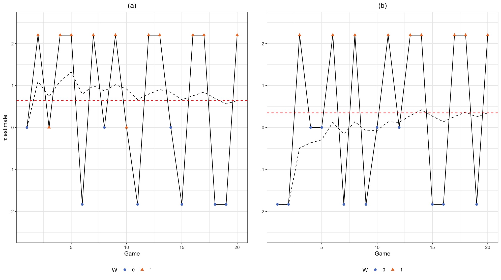
We estimate unit-specific average dynamic causal effects in the panel experiment conducted by Andreoni and Samuelson 2006. We focus on two randomly selected units in the experiment and construct estimates of their average $i,t$ -th lag- $0$ dynamic causal effect, $\tau_{i,t}(1,0;0)$ (Definition 5). Figure A16 shows the nonparametric estimates $\hat{\tau}_{i,t}(1,0;0)$ for $t\in[T]$ , for the two units. The figure also contains the nonparametric estimate of the average unit- $i$ lag- $0$ dynamic causal effect $\bar{\tau}_{i\cdot}(1,0;0)=\frac{1}{T}\sum_{t=1}^{T}\hat{\tau}_{i,t}(1,0;0)$ . The result shows that the point estimate of the average unit- $i$ lag- $0$ dynamic causal effect is positive for both units, suggesting that a larger value of $\lambda$ in the current game increases the likelihood of cooperation for both units. Since each unit only plays a total of twenty rounds, the estimated variance of these unit-specific estimators is quite large.

We next estimate period-specific, weighted average dynamic causal effects that pool information across units in order to gain precision. For each time period $t\in[T]$ , we construct estimates based on the nonparametric estimator of the weighted average time- $t$ , lag- $p$ dynamic causal effect $\bar{\tau}_{\cdot t}^{\dagger}(1,0;p)=\frac{1}{N}\sum_{i=1}^{N}\tau_{i,t}^{\dagger}(1,0;p)$ for $p=0,1,2,3$ . For each value of $p$ , the dashed black line in Figure A17 plots the estimates $\hat{\bar{\tau}}_{\cdot t}^{\dagger}(1,0;p)$ and the grey region plots a 95% pointwise conservative confidence band for the period-specific weighted average dynamic causal effects. For each value of $p$ , there appears to be some heterogeneity in the period-specific weighted causal dynamic causal effects across time periods.

To further investigate these dynamic causal effects, the solid blue line in Figure A17 plots the nonparametric estimator the total lag- $p$ weighted average causal effect $\bar{\tau}^{\dagger}(1,0;p)$ for $p=0,1,2,3$ , which further pools information across all units and time periods. The dashed blue lines plot the conservative confidence interval for the total lag- $p$ weighted average causal effect. See the main text for further discussion of the total lag- $p$ weighted average causal effect estimates.

		$\displaystyle Cov(u_{i,t-p}({\mathbf{w}},\tilde{\mathbf{w}};p),u_{i,t-p}(\bar{\mathbf{w}},\hat{\mathbf{w}};p)\|\mathcal{F}_{i,t-p-1})$
		$\displaystyle=Y_{i,t}(w_{i,1:t-p-1}^{obs},{\mathbf{w}})Y_{i,t}({w}_{i,1:t-p-1}^{obs},\bar{\mathbf{w}})Cov(Z_{i,t-p:t}({\mathbf{w}}),Z_{i,t-p:t}(\bar{\mathbf{w}})\|\mathcal{F}_{i,t-p-1})$
		$\displaystyle-Y_{i,t}(w_{i,1:t-p-1}^{obs},{\mathbf{w}})Y_{i,t}({w}_{i,1:t-p-1}^{obs},\hat{\mathbf{w}})Cov(Z_{i,t-p:t}({\mathbf{w}}),Z_{i,t-p:t}(\hat{\mathbf{w}})\|\mathcal{F}_{i,t-p-1})$
		$\displaystyle-Y_{i,t}(w_{i,1:t-p-1}^{obs},\tilde{\mathbf{w}})Y_{i,t}({w}_{i,1:t-p-1}^{obs},\bar{\mathbf{w}})Cov(Z_{i,t-p:t}(\tilde{\mathbf{w}}),Z_{i,t-p:t}(\bar{\mathbf{w}})\|\mathcal{F}_{i,t-p-1})$
		$\displaystyle Y_{i,t}(w_{i,1:t-p-1}^{obs},\tilde{\mathbf{w}})Y_{i,t}({w}_{i,1:t-p-1}^{obs},\hat{\mathbf{w}})Cov(Z_{i,t-p:t}(\tilde{\mathbf{w}}),Z_{i,t-p:t}(\hat{\mathbf{w}})\|\mathcal{F}_{i,t-p-1})$
		$\displaystyle=-Y_{i,t}(w_{i,1:t-p-1}^{obs},{\mathbf{w}})Y_{i,t}({w}_{i,1:t-p-1}^{obs},\bar{\mathbf{w}})+Y_{i,t}(w_{i,1:t-p-1}^{obs},{\mathbf{w}})Y_{i,t}({w}_{i,1:t-p-1}^{obs},\hat{\mathbf{w}})$
		$\displaystyle+Y_{i,t}(w_{i,1:t-p-1}^{obs},\tilde{\mathbf{w}})Y_{i,t}({w}_{i,1:t-p-1}^{obs},\bar{\mathbf{w}})-Y_{i,t}(w_{i,1:t-p-1}^{obs},\tilde{\mathbf{w}})Y_{i,t}({w}_{i,1:t-p-1}^{obs},\hat{\mathbf{w}})$

Abstract

1 Introduction

Notation:

2 Potential outcome panel and dynamic causal effects

2.1 Assignment panels and potential outcomes

Definition 1.

2.2 The potential outcome panel model

Assumption 1.

2.3 Assignment mechanism assumptions

Definition 2.

Definition 3.

Example 1.

Remark 2.1.

2.4 Dynamic causal effects

2.4.1 Lag-pp dynamic causal effects and average dynamic causal effects

Definition 4.

Definition 5.

Definition 6.

3 Nonparametric estimation and inference

3.1 Setup: adapted propensity score and probabilistic assignment

Assumption 2 (Probabilistic Assignment).

3.2 Estimation of the i,ti,t-th lag-pp dynamic causal effect

Theorem 3.1.

Proposition 3.1.

Remark 3.1.

3.3 Estimation of lag-pp average causal effects

Theorem 3.2.

Proposition 3.2.

3.4 Confidence intervals and testing for lag-pp average causal effects

4 Estimation in a linear potential outcome panel

Definition 7.

4.1 Interpreting the unit fixed effects estimator

Proposition 4.1.

Example 2.

4.2 Interpreting the two-way fixed effects estimator

Proposition 4.2.

5 Simulation Study

5.1 Simulation design

5.2 Normal approximations and size control

5.3 Rejection rate

6 Empirical application in experimental economics

6.1 Inference on total lag-pp weighted average dynamic causal effects

7 Conclusion

References

Appendix A Proofs of main results

Proof of Theorem 3.1

Lemma A.1.

Proof.

Proof of Proposition 3.1

Lemma A.2.

Proof of Theorem 3.2

Proof of Proposition 3.2

Proof of Proposition 4.1

Proof of Proposition 4.2

Appendix B Additional theoretical results

B.1 Prediction decomposition of the adapted propensity score

Lemma B.1.

Proof.

B.2 Estimation as a repeated cross-section

Proposition B.1.

Proof.

Appendix C Additional simulation results

C.1 Additional simulations for the estimator of the total average dynamic causal effects

Quantile-quantile plot for the normal approximation:

Simulation results for the estimator of the lag-11 total weighted average dynamic causal effect, τ¯†​(1,0,1)\bar{\tau}^{\dagger}(1,0;1):

C.2 Simulations for the estimator of the time-tt average dynamic causal effects

Normal approximations and size control:

Rejection rates:

Simulation results for the estimator of the lag-11, time-tt weighted average dynamic causal effect, τ¯⋅,t†​(1,0,1)\bar{\tau}^{\dagger}_{\cdot,t}(1,0;1):

C.3 Simulations for the estimator of the unit-ii average dynamic causal effects

Normal approximations and size control:

Rejection rates:

Simulation results for the estimator of the lag-11, unit-ii weighted average dynamic causal effect, τ¯i,⋅†​(1,0,1)\bar{\tau}^{\dagger}_{i,\cdot}(1,0;1):

Appendix D Additional empirical results

D.1 Analysis of unit and time-specific average dynamic causal effects

2.4.1 Lag- $p$ dynamic causal effects and average dynamic causal effects

3.2 Estimation of the $i,t$ -th lag- $p$ dynamic causal effect

3.3 Estimation of lag- $p$ average causal effects

3.4 Confidence intervals and testing for lag- $p$ average causal effects

6.1 Inference on total lag- $p$ weighted average dynamic causal effects

Simulation results for the estimator of the lag- $1$ total weighted average dynamic causal effect, $\bar{\tau}^{\dagger}(1,0;1)$ :

C.2 Simulations for the estimator of the time- $t$ average dynamic causal effects

Simulation results for the estimator of the lag- $1$ , time- $t$ weighted average dynamic causal effect, $\bar{\tau}^{\dagger}_{\cdot,t}(1,0;1)$ :

C.3 Simulations for the estimator of the unit- $i$ average dynamic causal effects

Simulation results for the estimator of the lag- $1$ , unit- $i$ weighted average dynamic causal effect, $\bar{\tau}^{\dagger}_{i,\cdot}(1,0;1)$ :