Electroweak fermion triangle loop contributions
to the muon anomalous magnetic moment revisited

A discrepancy of $3.3\sigma$ still remains between experiment and the standard model (SM) prediction for the muon anomalous magnetic moment $a_{\mu}\equiv(g_{\mu}-2)/2$ PDG2018. The calculations of two-loop contributions to $a_{\mu}$ due to the electroweak interactions of the SM were completed quite some time ago KKSS1992; PPdeR1995; CKM1995; CKM1996 and recently the numerically evaluated results of full two-loop electroweak corrections were presented INY2019. For more references, see Ref.PDG2018. Two-loop electroweak corrections are expressed as the form

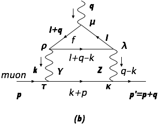
Among the two-loop electroweak contributions there are an interesting subset of which are induced by triangle loops of charged fermions connected to the muon line by a photon and a $Z$ boson. The relevant Feynman diagrams are shown in Fig.1. The fermionic triangle subdiagrams in Fig.1 have the Adler-Bell-Jackiw $VVA$ anomaly, which cancels out when all the fermions in each generation are included. The analysis of this subset of diagrams was first made by Kukhto et al. KKSS1992 (KKSS). They used a simplified version of the $Z\gamma\gamma$ vertex function by Adler Adler1969 and Rosenberg Rosenberg1963 for the fermionic triangle subdiagrams and found that the loop contributions of leptons, i.e., $e,\mu$ and $\tau$, were enhanced by large logarithms of the form $\ln(m_{Z}/m_{\mu})$ or $\ln(m_{Z}/m_{\tau})$. Then followed the studies of quark loop contributions PPdeR1995; CKM1995.

In the calculation of two-loop electroweak contributions to $a_{\mu}^{\rm EW}$, the authors of CKM1995; CKM1996 employed the asymptotic expansion method and used the ’t Hooft-Feynman gauge. Then in Ref.CM2017, Czarnecki and Marciano, coauthors of Refs.CKM1995; CKM1996, illustrated the asymptotic expansion method in computing the triangle loop diagrams in Fig.1 with $f=$ top quark, since in this case there appear two large ratios of masses, $m_{t}^{2}/m_{Z}^{2}$ and $m_{Z}^{2}/m_{\mu}^{2}$. The result is made up of $\Delta C_{Z}$ and $\Delta C_{G}$ which are given in Eqs.(9) and (10), respectively, of Ref.CM2017. $\Delta C_{G}$ is the contribution of the neutral Goldstone boson.

Actually the top quark (more generally, a charged fermion) triangle loop contributions can be calculated exactly, the results of which in the unitary gauge were already given in Eqs.(13)-(15) of Ref.PPdeR1995, in the form of parametric representation with five Feynman parameters. In this letter I reexamine the contributions to $a_{\mu}$ from the fermion triangle-loop diagrams depicted in Fig.1 in the unitary gauge and show that with use of the anomalous axial-vector Ward identity, the calculation in the unitary gauge exactly coincides with the one in the ’t Hooft-Feynman gauge. The part which arises from the ordinary axial-vector Ward identity corresponds to the contribution of the neutral Goldstone boson. Then, for the top-quark contribution, the one-parameter integral form is obtained up to the order of $m_{\mu}^{2}/m_{Z}^{2}$. The results are compared with those obtained by the asymptotic expansion method.

The muon state before and after the interaction with a photon field with momentum $q$ satisfies the following on-shell conditions:

where $m_{\mu}$ is a muon mass. In the following calculation we put $q^{2}=0$ and then the above on-shell conditions lead to $p\cdot q=0$. It is well-known that the contributions of $VVV$ terms in the fermionic triangle subdiagrams in Fig.1 (a) and (b) mutually cancel by virtue of Furry’s theorem while the $VVA$ terms have the Adler-Bell-Jackiw anomaly. Then we use the $Z\gamma\gamma$ vertex function derived by Adler Adler1969 and Rosenberg Rosenberg1963 for the fermionic triangle subdiagrams, which reads in terms of the momenta shown in Fig.1 as,

where $m_{f}$ is a fermion mass in the loop and $\epsilon^{\lambda\mu\rho q}=\epsilon^{\lambda\mu\rho\alpha}q_{\alpha}$, etc.. The convention $\epsilon^{0123}=-\epsilon_{0123}=1$ is used which agrees with Peskin and Schroeder PS1995 and not with Adler and Rosenberg Adler1969; Rosenberg1963 nor with KKSS KKSS1992. Note that the above expression is the full-version of the $Z\gamma\gamma$ vertex function with $q^{2}=0$. In Ref.KKSS1992, KKSS used a simplified version of $Z\gamma\gamma$ vertex function obtained from the full-version (3) by keeping, in the numerator, only the terms linear in the external photon momenta $q$ and discarding the $k\cdot q$ term in the denominator. The full-version $R^{\mu\rho\kappa}(q,-k,k-q)$ satisfies the electromagnetic current conservation, $q_{\mu}R^{\mu\rho\lambda}(q,-k,k-q)=0$ and $k_{\rho}R^{\mu\rho\lambda}(q,-k,k-q)=0$, and the anomalous axial-vector Ward identity

The first term is the Adler-Bell-Jackiw $VVA$ anomaly and independent of the fermion mass $m_{f}$ in the loop, while the second term corresponds to the ordinary axial-vector Ward identity and is proportional to $m_{f}^{2}$.

The calculation of the lower-loop in Fig.1 is performed by using the $Z$-boson propagator in the unitary gauge,

The contraction of $(k-q)_{\lambda}$ and the $Z\gamma\gamma$ vertex function gives the anomalous axial-vector Ward identity in (4). The anomaly term generates a divergence in the loop integral. But it does not depend on the fermion and thus, in the SM, the contributions of the anomaly terms cancel out when all the fermions in each generation are included PPdeR1995. Hence in the following we omit the anomaly term. The calculation proceeds by making full use of an identity

and the on-shell conditions (2). Discarding the terms with $\gamma_{\mu}$ and picking only those with $p_{\mu}$ and $q_{\mu}$, the remaining terms are found to be proportional to $(2p+q)_{\mu}$. Then the $y$-integration and the symmetrization in $x$ variable, i.e., $f(x)\rightarrow[f(x)+f(1-x)]/2$ are made.

Finally the following expressions are obtained for the triangle loop contribution of a fermion $f$ in the integral form with four Feynman parameters,

where

with $a\equiv x(1-x)$, $\lambda_{f}\equiv m_{f}^{2}/m_{Z}^{2}$ and $\kappa\equiv m_{\mu}^{2}/m_{Z}^{2}$; $N_{c}^{f}$, $Q_{f}$ and $I_{3f}$ are the color factor, the electric charge and the third component of weak isospin of the fermion $f$, respectively, with $N_{c}^{f}=3(1)$ for quarks (leptons). These are exact results, and $A_{\gamma Z}(\lambda_{f},\kappa)$ and $B_{\gamma Z}(\lambda_{f},\kappa)$ are equivalent to ${\cal F}[m_{f}^{2}/m_{\mu}^{2},M_{Z}^{2}/m_{\mu}^{2}]$ in Eq.(14) and ${\cal G}[m_{f}^{2}/m_{\mu}^{2},M_{Z}^{2}/m_{\mu}^{2}]$ in Eq.(15) of Ref.PPdeR1995, respectively. Having the expressions given in (8) and (9), it is easy to perform further integrations w.r.t. the Feynman parameters $z_{2}$, $z_{3}$, and $z_{4}$. The term $A_{\gamma Z}(f)$ comes from the $g_{\lambda\kappa}$ part of the $Z$-boson propagator (5). On the other hand, the $B_{\gamma Z}(f)$ term arises from the ordinary axial-vector Ward identity, and thus is multiplied by the factor $\lambda_{f}$ in (7). Due to this factor, $B_{\gamma Z}(f)$ is only relevant for the case $f=$ top quark PPdeR1995. It is interesting to note that the expression of $A_{\gamma Z}(f)$ turns out to be the same as the one given by KKSS in Eq.(4.10) of Ref.KKSS1992, which was derived by using the simplified version of $Z\gamma\gamma$ vertex function.

Now consider the calculation of the same diagrams in Fig.1 in the ’t Hooft-Feynman gauge. The $Z$-boson propagator in the ’t Hooft-Feynman gauge is given by

which is the same form as the $g_{\lambda\kappa}$ part of the $Z$-boson propagator in the unitary gauge in (5). Hence the contribution generated from the $Z$-boson propagator in the ’t Hooft-Feynman gauge is expressed as $A_{\gamma Z}(f)$ in (8). In addition we need to consider the contribution generated from the neutral Goldstone boson $G^{0}$. The relevant diagrams are obtained from Fig.1 (a) and (b) with replacement of the $Z$-boson propagator by that of $G^{0}$. Also the axial-vector couplings of the $Z$-boson are replaced by the pseudo-scalar couplings of $G^{0}$ to the fermion in the loop and the muon. The loop-integral of the fermionic triangle subdiagrams in Fig.1 (a) and (b) where the axial-vector vertex $\gamma^{\lambda}\gamma_{5}$ is replaced by the pseudo-scalar vertex $m_{f}\gamma_{5}$ gives

which is just one half of the second term of (4) (an ordinary axial-vector Ward identity). Now attaching the pseudo-scalar vertex $m_{\mu}\gamma_{5}$ to the muon line, the lower-loop integral is made and the following exact result is obtained for the contribution generated from the neutral Goldstone boson $G^{0}$:

where

The expressions of $B_{\gamma Z}(f)$ and $B_{\gamma G^{0}}(f)$ look different at first glance but actually they are equivalent. Take the difference and we see that it vanishes after the integration w.r.t. the variables $z_{2}$, $z_{3}$ and $z_{4}$. Now it is clear that the calculation in the unitary gauge exactly coincides with the one in the ’t Hooft-Feynman gauge. The part which arises from the ordinary axial-vector Ward identity in the unitary gauge corresponds to the contribution of the neutral Goldstone boson.

For the case $m_{f}^{2}\gg m_{\mu}^{2}$, the integrations of $A_{\gamma Z}(f)$ and $B_{\gamma Z}(f)(=B_{\gamma G^{0}}(f))$ w.r.t. the variables $z_{2}$, $z_{3}$, and $z_{4}$ are easily made up to ${\cal O}(\kappa)$. The results are

where

The expression of $\lambda_{f}{\widetilde{B}}_{\gamma Z}(f)$ appeared already in the literature BZ1990; CCCK2001; CCK2001; CM2017 as the integral representation for the Barr-Zee diagrams. In the case of top quark, and thus $N_{c}^{t}Q_{t}^{2}I_{3t}=\frac{2}{3}$ and $\lambda_{t}\simeq 3.6$, we expand $\frac{1}{a-\lambda_{t}}$ as

and we obtain after the $x$-integration

We see that the above equations (18) and (19) reproduce the results of the asymptotic expansion method, $\Delta C_{Z}$ and $\Delta C_{G}$, which are given in Eqs.(9) and (10) of Ref.CM2017. In addition, the subleading ${\cal O}(1/\lambda_{t}^{2})$ terms and the nonleading ${\cal O}(\kappa)$ terms are included, respectively, in (18) and (19), which may serve as another check on the asymptotic expansion method.

For the contribution of top-quark $C_{\gamma Z}(t)$, the integral form of $\frac{8}{5}\Bigl({\widetilde{A}}_{\gamma Z}(t)-\lambda_{t}{\widetilde{B}}_{\gamma Z}(t)\Bigr)$ gives  -5.134 with $\lambda_{t}=3.6$, while the use of the leading ${\cal O}(1)$ and subleading ${\cal O}(1/\lambda_{t})$ terms in the expansions in (18) and (19), which is the result of the asymptotic expansion method, $(\Delta C_{D}+\Delta C_{G})$, given in Eq.(11) of Ref.CM2017, leads to  -5.140. Agreement is excellent and we see that the asymptotic expansion method works just fine for the case of top quark triangle loop diagrams. The integral form of ${\widetilde{A}}_{\gamma Z}(f)$ in (16) is still applicable to estimate $C_{\gamma Z}(f)$ for the contributions from the loops of $b$ quark, $\tau$ lepton and $c$ quark. Or a formula ${\widetilde{A}}_{\gamma Z}(f)\approx(3/2)(-2-\ln\lambda_{f})$ can be used since $\lambda_{f}\ll 1$ for $f=b,\tau,c$. On the other hand, for the light quarks, i.e., $u$, $d$ and $s$ quarks, there is the issue of how to properly treat their triangle loop diagrams PPdeR1995; KPdeRP2002; CMV2003. For the contributions to $a_{\mu}$ from the muon and electron triangle loop diagrams, we arrive at the same formulae given by KKSS (Eqs.(4.11) and (4.12) of Ref.KKSS1992) since $A_{\gamma Z}(f)$ in (8) is the same expression as the one derived by them.

In summary, the two-loop electroweak contributions to $a_{\mu}$ from fermion triangle diagrams connected to the muon line by a photon and a $Z$-boson depicted in Fig.1 can be calculated without approximations. It is shown that the calculation in the unitary gauge exactly coincides with the one in the ’t Hooft-Feynman gauge. The part generated from the ordinary axial-vector Ward identity in the unitary gauge corresponds to the contribution of the neutral Goldstone boson in the ’t Hooft-Feynman gauge. For the top-quark contribution, the one-parameter integral form is obtained up to the order of $m_{\mu}^{2}/m_{Z}^{2}$. The results are compared with those obtained by the asymptotic expansion method. We see that numerically agreement is excellent. And yet still remains the discrepancy of 3.3$\sigma$ between experiment and theory for $a_{\mu}$.