Optimal exploitation of the resource in remote state preparation

To unify the previous studies with the current one, the RSP protocol is modeled as an encoding-decoding mechanism that exploits the shared resource state and one classical bit to perform the RSP task as depicted in Fig. 1.

In RSP protocol, Alice aims to transmit the signal state $\left|{{\psi_{s}}}\right\rangle$, that in the Bloch sphere representation, corresponds to a unit vector ${\hat{s}}$. According to the protocol, the signal state is selected from a certain great circle characterized by its normal vector ${\hat{\beta}}$ (in our notation $\hat{s}\in\mathrm{GC}(\hat{\beta})$). The parameterization of $\hat{s}\in\mathrm{GC}(\hat{\beta})$ in the spherical coordinate system is given in Appendix A.3.

To perform the RSP task, Alice and Bob exploit shared resource state ${\rho_{AB}}$ as a passive quantum channel, where state ${\rho_{AB}}$ , in its general form can be written in two-qubit Bloch vector representation as

in which $\vec{a}$ and $\vec{b}$ are the local Bloch vectors of Alice’s and Bob’s state respectively, ${E_{ij}}=\mathrm{Tr}[\sigma_{i}\otimes\sigma_{j}\rho_{AB}]$ are the elements of correlation matrix $E$, $I=\mathrm{diag}[1,1,1,1]$ denotes an equal mixture of the four Bell states ($\left|{{\psi^{\pm}}}\right\rangle=({{\left|{01}\right\rangle\pm\left|{10}\right\rangle)}\mathord{\left/{\vphantom{{\left|{01}\right\rangle\pm\left|{10}\right\rangle)}{\sqrt{2}}}}\right.\kern-1.2pt}{\sqrt{2}}}$ and $\left|{{\varphi^{\pm}}}\right\rangle=({{\left|{00}\right\rangle\pm\left|{11}\right\rangle)}\mathord{\left/{\vphantom{{\left|{00}\right\rangle\pm\left|{11}\right\rangle)}{\sqrt{2}}}}\right.\kern-1.2pt}{\sqrt{2}}}$) and $\vec{\sigma}=({\sigma_{x}},{\sigma_{y}},{\sigma_{z}})$ where ${\sigma_{i}}(i=x,y,z)$ are Pauli operators.

In this general model, after restricting the encoding and decoding operators to the class of projective measurements and unitary operators, respectively; the encoding and decoding phases of the protocol reads as follows:

Encoding Phase: Alice encodes the known signal state into Bob’s qubit by performing a projective measurement $\{\left|{\pm\alpha}\right\rangle\left\langle{\pm\alpha}\right|\}$ on qubit A. This measurement is parameterized by ${\{{\hat{\alpha}_{m}}\}_{m=1,2}}$, where ${\hat{\alpha}_{1}}=+\hat{\alpha}$, ${\hat{\alpha}_{2}}=-\hat{\alpha}$ and $\hat{\alpha}=({\alpha_{x}},{\alpha_{y}},{\alpha_{z}})$ is a real unit vector in the Bloch sphere representation. Depending on the output of Alice’s measurement, the local Bloch vector of Bob is projected into vector

with probability

where $E^{T}$ is the transpose of the correlation matrix $E$. To activate the quantum channel, Alice should send via a supporting classical channel her measurement result to Bob.

Decoding Phase: To decode the signal state, depending on the received classical bit, Bob applies a local unitary transformation, i.e. he applies $U_{m}$ on his qubit when receives the classical bit $m$. As a result, after receiving the classical bit $m$ and applying the corresponding unitary transformation, Bob decodes the Bloch vector of transmitted state as

where $R_{m}(\hat{n}_{m},\gamma_{m})$ is a unique rotation satisfying $U_{m}(\vec{v}.\vec{\sigma})U_{m}^{\dagger}=(R_{m}\vec{v}).\vec{\sigma}$, that rotates any arbitrary Bloch vector $\vec{v}$ by angle $\gamma_{m}$ about the direction $\hat{n}_{m}$. The explicit form of $R_{m}$ is given in Appendix A.1 and the whole scenario is depicted in Fig. 2.

After classical communication of Alice’s measurement outcome and corresponding decoding operation performed by Bob, by using Eq.(4), Eq.(5) and Eq.(6), the averaged Bloch vector of transmitted state is obtained as

The TE of the protocol can be quantified using the standard linear fidelity as follows

where ${\rho^{(\vec{r})}}$ is the average prepared state in Bob’s site. Fidelity $F$ in general is a function of input signal state, encoding-decoding and resource state parameters, i.e.

To explore the actual relation between the performance of the protocol and the resource state parameters, all encoding-decoding parameters and the input state in Eq.(9) should be traced out in a suitable and meaningful manner. The resulting relation then provides a correspondence between the performance of RSP and the resource state used to perform the task. In the next section we will have an overview of the previous approaches that quantify the performance of the protocol in terms of the resource parameters.

In the first approach, to quantify the performance of RSP, a quadratic fidelity, known as payoff, was defined as $P={(\vec{r}.\hat{s})^{2}}$ that after applying some reasonable procedures relates the TE of the protocol to the geometric discord of resource state Dakić et al. 2012. In this approach, for every ${\rho_{AB}}$, the decoding strategy of the protocol is chosen as same as the strategy employed in the standard RSP protocol. In the standard protocol, Alice and Bob agree on a pre-shared direction, characterized by the vector $\hat{\beta}$. Alice chooses her input states from $\hat{s}\in\mathrm{GC}(\hat{\beta})$ and Bob’s decoding operators are ${R_{1}}={R_{1}}(\hat{\beta},0)$ and ${R_{2}}={R_{2}}(\hat{\beta},\pi)$ that correspond to the rotation of Bloch vectors in Bob’s coordinate system about the pre-shared $\hat{\beta}$ direction by $0$ and $\pi$ radian, respectively. After fixing this decoding strategy, for every $\hat{s}\in\mathrm{GC}(\hat{\beta})$ Alice chooses a projective measurement that maximizes the payoff. This maximized payoff is given by

In the next step, the maximized payoff is averaged over all $\hat{s}\in\mathrm{GC}(\hat{\beta})$, which gives

where ${\cal P}$ is the resulting TE for the great circle corresponding to the normal vector ${\hat{\beta}}$. Finally, ${\cal P}({\hat{\beta}})$ is minimized over the direction ${\hat{\beta}}$ and the resulting minimum payoff is given by

with

where $\lambda_{1}^{2}$, $\lambda_{2}^{2}$ and $\lambda_{3}^{2}$ are eigenvalues of the matrix ${E^{T}}E$. Surprisingly, for a broad class of states this expression is equal to the geometric discord of ${\rho_{AB}}$. This result showed that in the worst-case scenario, the TE of the protocol is not less than quantum discord, i.e. discord acts as optimal resource for the RSP protocol.

However, as remarked in Kanjilal et al. 2018, if a zero discord state is used as a resource for RSP, according to the mentioned approach the most one can claim is the existence of at least one great circle, say $\hat{\beta}_{0}$, for which RSP cannot be implemented for all $\hat{s}\in\mathrm{GC}(\hat{\beta}_{0})$. Nevertheless, zero-discord states may still be of use as a resource for an effective RSP corresponding to the other great circles. Actually, since quantum discord is equal to the minimum of the average payoff, therefore, discord cannot quantify the effectiveness of the resource state in the RSP protocol for any given $\hat{\beta}$. To eliminate this drawback, reference Kanjilal et al. 2018 suggested that instead of minimizing the averaged payoff over $\hat{\beta}$ that corresponds to the worst-case scenario, ${\cal P}({\hat{\beta}})$ should be averaged over all the great circles characterized by $\hat{\beta}$. Therefore, one obtains

Accordingly, if $\cal Q$ vanishes, then ${\cal P}({\hat{\beta}})=0$ for all $\hat{\beta}$ and no signal state can be remotely prepared closer to the signal state other than the maximally mixed state. Therefore, nonvanishing of the quantity $\cal Q$ can be considered as a necessary condition for the effectiveness of RSP protocol for a given resource state.

Finally, by considering the recently introduced measures of SCMUB for Bell diagonal states ($\vec{a}=\vec{b}=0$), the following analytical relationship between $C_{3}$ and $\cal Q$ was obtained

where $C_{3}$ is simultaneous correlations in three mutually unbiased bases introduced in Guo and Wu 2014 and $h$ is the Shannon function. Interestingly, $C_{3}$ is a monotonically increasing function of $\cal Q$. Notice that the quantity $\cal Q$ does not vanish for zero-discord Bell-diagonal states, which are of the form $E=\mathrm{diag}[{\lambda},{0},{0}]$, i.e. zero-discord states are useful as a resource for implementing RSP for a class of signal states pertaining to at least one choice of $\mathrm{GC}(\hat{\beta})$.

The approaches mentioned in this section use the payoff as quantifier of the TE in RSP protocol. However, there is a need to justify the use of payoff as a figure of merit to quantify the performance of the protocol. This issue is the subject of the following subsection.

The payoff function, defined as $P={(\vec{r}.\hat{s})^{2}}$, has been used in the previous works to quantify the performance of RSP. However, neither of these works have discussed about the origin of this definition and justification of using payoff as quantifier of the TE in RSP. Such a discussion seems necessary, especially if one considers two states corresponding to the Bloch vectors $+{{\vec{r}}_{0}}$ and $-{{\vec{r}}_{0}}$ (with $\vec{r}.\hat{s}\geq 0$), respectively. In terms of the linear fidelity, that evidently is a correct figure of merit to quantify the TE of RSP, the states ${\rho^{(+{{\vec{r}}_{0}})}}$ and ${\rho^{(-{{\vec{r}}_{0}})}}$ have different fidelities with respect to a reference signal state, say $\left|{{\psi_{{{\hat{s}}_{0}}}}}\right\rangle$; i.e. $F\left({\pm{{\vec{r}}_{0}},{{\hat{s}}_{0}}}\right)=\frac{{1\pm{{\vec{r}}_{0}}.{{\hat{s}}_{0}}}}{2}$. However, in terms of payoff, clearly we have $P\left({-{{\vec{r}}_{0}},{{\hat{s}}_{0}}}\right)=P\left({+{{\vec{r}}_{0}},{{\hat{s}}_{0}}}\right)$. This means that payoff is unable to distinguish between orthogonal states ${\rho^{(-{{\vec{r}}_{0}})}}$ and ${\rho^{(+{{\vec{r}}_{0}})}}$ for all ${{\vec{r}}_{0}}$. However, we show that after maximizing the payoff over the encoding strategies, this drawback is eliminated. Let us start with the linear fidelity

where ${\vec{r}}$ is given by Eq.(7) and ${\hat{s}}$ is the Bloch vector of the signal state. In Appendix A.2 it is shown that after maximizing the linear fidelity over the encoding parameters, i.e. maximizing over ${\hat{\alpha}}$, the maximized linear fidelity is given by

where $R_{i}^{T}$ is the transpose of the matrix $R_{i}\,(i=1,2)$ and $||{\vec{V}}||$ is the Euclidean norm of the vector ${\vec{V}}$.

Now, we show that under one of the following conditions, payoff as well as the linear fidelity can successfully quantify the TE of RSP:

(C1)

For $\{{R_{1}}={R_{1}}({\hat{\beta},0}),{R_{2}}={R_{2}}({\hat{\beta},\pi})\}$.

(C2)

For $\vec{b}=0$.

Condition (C1) corresponds to the standard decoding strategy employed in Dakić et al. 2012 and condition (C2) corresponds to the resource states with maximally mixed marginal for Bob’s qubit. From Eq.(17) it is evident that under one of conditions (C1) or (C2) the first term of Eq.(17) vanishes and a maximized encoding strategy leads to ${F_{\mathrm{max}}}\geq\frac{1}{2}$. A comparison between Eq.(16) and Eq.(17) shows that, when one of the above conditions is satisfied, just by using a maximized encoding strategy, the Bloch vector of the prepared state always overlaps with the Bloch vector of the signal state by an angel less than $\frac{\pi}{2}$ radian. As a result, one can define the payoff function as

with the guarantee that after using an optimal encoding strategy, $\vec{r}.\hat{s}\geq 0$ in complete agreement with ${\left({\vec{r}.\hat{s}}\right)^{2}}\geq 0$, i.e. with an optimized encoding strategy, the state ${\rho^{(-{{\vec{r}}_{0}})}}$ will never be prepared in Bob’s site to be mistaken as ${\rho^{(+{{\vec{r}}_{0}})}}$ by the payoff function. Therefore, under conditions (C1) or (C2), the payoff function and the linear fidelity have similar behavior and both of them can be used to quantify the performance of RSP. More interestingly, as we will see in the next section, under one of the mentioned conditions, the averaged maximum linear fidelity can be expressed in terms of the averaged maximum payoff function and vice versa.

Before concluding this section, we remark that the argument employed in [14] for invalidating the payoff as figure of merit for the TE of RSP needs more careful consideration. The argument reads as follows Horodecki et al. 2014:

”Consider a case of the protocol in which Bob, regardless of the Alice message, produces at random a pure state with a Bloch vector belonging to the ${\hat{s}}$ plane. Employing quadratic fidelity proposed in Dakić et al. 2012 one obtains

$$\begin{split}&{\cal P}=\mathop{\min}\limits_{\hat{\beta}}{\left({\hat{r}.\hat{s}}\right)^{2}}={\left({\hat{r}.\hat{s}}\right)^{2}}=\smallint d\hat{s}{\left({\hat{r}.\hat{s}}\right)^{2}}\\ &\ \ \ =\frac{1}{{2\pi}}\mathop{\smallint}\nolimits_{0}^{2\pi}d\varphi{\cos^{2}}\left(\varphi\right)=\frac{1}{2},\end{split}$$

(19)

where the invariance of the measure on the unit circle is used. Because this fidelity is higher than those considered in Dakić et al. 2012 ( $1/9$ and $1/25$ for separable and entangled state considered in Dakić et al. 2012 respectively), it may seem that the random protocol is better choice than more sophisticated strategies. However, this is only because of misleading choice of protocol fidelity.”

However, it is necessary to note that according to the argument presented in the initial paragraphs of this section, only under the optimized encoding strategy the payoff can be regarded as a valid figure of merit to quantify the TE of RSP. Obviously the guessing protocol introduced in the above argument doesn’t meet this condition. As a result, when averaging the TE over the unit vector ${\hat{s}}$, the terms that have negative contributions to the linear fidelity, contribute as positive terms in the payoff that leads to misleading results such as the result obtained in the guessing protocol.

Therefore, to some extent the intuition behind the paper Dakić et al. 2012 is correct and the challenging result of Dakić et al. 2012 cannot be due to the employment of payoff as was claimed by Horodecki et al. 2014. However, this approach employs a non-optimal decoding strategy. In the next section, the TE of RSP in the fully optimized scenario is investigated.

In this section we restrict the encoding and decoding maps to the classs of projective measurements and unitary operators, respectively and evaluate the TE of RSP in terms of both quadratic and linear fidelities in the fully optimized scenario (see Fig. 1). It is important to note that the optimization over the decoding strategies differs form the optimization over the encoding strategies in the sense that Alice knows the state she intends to transmit and consequently $\forall\hat{s}\in\mathrm{GC}(\hat{\beta})$, she can choose the optimal measurement. However, Bob doesn’t know the signal states and for any given $\hat{\beta}$, the most he can do, is to fix a decoding strategy that maximizes the average fidelity, i.e. for every $\hat{\beta}$, the TE in terms of the linear fidelity should be defined as follows

where ${\left\langle\bullet\right\rangle_{{}_{\hat{s}\in\mathrm{GC}(\hat{\beta})}}}$ stands for averaging the argument over $\hat{s}\in\mathrm{GC}(\hat{\beta})$. The TE in terms of payoff is defined in a similar manner, i.e.

To have a comprehensive approach in recognizing the role of resource state in the TE of RSP it is constructive to define the following expressions,

Similar expressions are also defined for payoff. The above expressions also provide a framework for comparing the previous works with the current scenario.

The analytical solution to evaluate the above expressions seems impractical at least by formal mathematical analysis methods. Ingenious methods may be later considered by mathematically oriented experts of the field. However, a fully numerical method is also impractical due to the very long execution time of the algorithms. Here, a combined approach is employed, i.e. the optimization over the encoding operators for the linear and quadratic fidelities and also averaging over the input signal states in the quadratic fidelity are performed analytically. Finally, the maximization over the decoding operators and the optimization over the direction ${\hat{\beta}}$ are performed numerically. All numerical analysis are performed using the standard optimization tools of Mathematica. See Appendix for details of the analytical and numerical methods. The problem is investigated for general resource states. The results show that in the optimized encoding-decoding scenario, the TE of RSP for all states ${\rho_{AB}}(\vec{a},\vec{b},E),$ in terms of the linear fidelity is independent of the direction ${\hat{\beta}}$ and is expressed in terms of the resource state parameters as follows

where $S2$ refers to the surface of the Bloch sphere and

where $\lambda_{1}^{2}$, $\lambda_{2}^{2}$ and $\lambda_{3}^{2}$ are eigenvalues of the matrix ${E^{T}}E$. Fig. 3 illustrates the numerical results for Bell-diagonal states corresponding to all values of ${\lambda_{1}}$ and ${\lambda_{2}}$ belonging to the physical regions and four different values of ${\lambda_{3}}$, i.e. ${\lambda_{3}}=0.00,\;0.25,\;0.50,\;0.75$. The physical regions are obtained from the positivity constraint of the density matrix ${\rho_{AB}}$. Appendix A.5 gives these physical regions in terms of four inequalities. Note that according to Eq.(17), the TE is independent of the local Bloch vector of Alice’s state. Also, the TE is independent of the local Bloch vector of Bob’s state, because after averaging the maximized linear fidelity over the unit vector $\hat{s}\in\mathrm{GC}({\hat{\beta}})$, the first term in right-hand side of Eq.(17) vanishes. Hence, the results of Fig. 3, are valid for all states ${\rho_{AB}}(\vec{a},\vec{b},E)$.

To investigate the TE of RSP in terms of payoff, one should be careful that according to the results of Sec.III.3, in the fully optimized scenario, only for states ${\rho_{AB}}(\vec{a},\vec{b},E)$ with $\vec{b}=0$ payoff is a valid figure of merit to quantify the performance of the protocol. To clarify the justification of this assumption note that, one always can assume that the receiver of the signal state (say Bob) be the distributor of the resource state. Therefore, Bob that starts from a maximally entangled state has control over his qubit with $\vec{b}=0$ and the Bloch vector of other part, i.e. $\vec{a}$, that is transmitted and affected by the channel, according to Eq.(17), doesn’t contribute to the TE of the protocol. Therefore, in these demanding scenarios, payoff as well as the linear fidelity can successfully quantify the TE of the protocol.
The numerical results (see Fig. 3) show that in the optimized encoding-decoding scenario, the TE of RSP for all states ${\rho_{AB}}(\vec{a},\vec{b},E)$ with $\vec{b}=0$ in terms of payoff is independent of the direction ${\hat{\beta}}$ and is expressed in terms of the resource state parameters as follows

where, $\cal D$ is given by Eq.(24). From Eq.(23) and Eq.(25) it is evident that the relation between the linear and quadratic fidelities for states ${\rho_{AB}}(\vec{a},\vec{b},E)$ with $\vec{b}=0$ is obtained as follows

This relation is also valid for standard decoding strategy, without requiring $\vec{b}=0$.

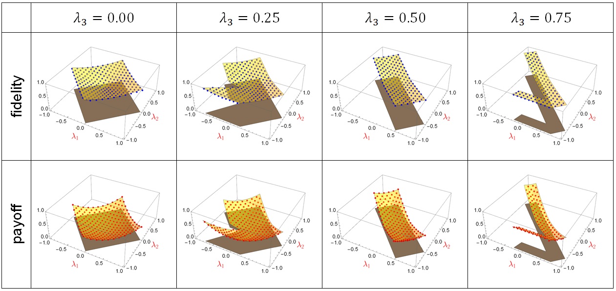
It is worthy to note that, since the TE in terms of the linear and quadratic fidelities are independent of the direction $\hat{\beta}$, we will have ${{\cal F}_{\mathrm{min}}}={{\cal F}_{\mathrm{max}}}={{\cal F}_{\mathrm{avg}}}$ for the linear fidelity and ${{\cal P}_{\mathrm{min}}}={{\cal P}_{\mathrm{max}}}={{\cal P}_{\mathrm{avg}}}$ for the quadratic fidelity. This interesting result shows that by an optimized encoding-decoding strategy, all great circles exploit the resource state equally. Also, from Eq.(23) or Eq.(25) it is evident that any nonproduct state can contribute to the process of RSP, i.e. correlations more than discord serve as a resource for RSP.

Before concluding this section, let us have a comparison between the result obtained in approach Dakić et al. 2012 and result of the present approach. Denoting the obtained fidelity considered in approach Dakić et al. 2012 by ${\cal F}_{\mathrm{min}}^{\left(1\right)}$, and also the minimum fidelity obtained in the fully optimized scenario by ${\cal F}_{\mathrm{min}}^{\left(3\right)}$; one can check the following inequality,

The strict inequality can be easily understood, as in the new approach a full optimization is carried out. However, the equality are not obvious and need more consideration that is investigated in the next section.

Considering Eq.(26), the comparison between Eq.(12) and Eq.(23) shows that for states with isotropic correlation matrix, i.e. for states with $E=\pm\lambda I$, the TE of RSP resulting from standard and optimal decoding strategies coincide. Therefore, for isotropic states, $\forall\;\hat{\beta}\in S2$ the decoding considered in Dakić et al. 2012 and Kanjilal et al. 2018, i.e. the decoding strategy used in the standard RSP protocol, is an optimal decoding strategy. Besides this, the comparison between Eq.(13) and Eq.(24) shows that for isotropic states when standard encoding-decoding strategy is employed, quantum discord truly is optimal resource of RSP.

One important class of isotropic states are Werner states with

Werner states are a family of one parameter states with $\vec{a}=\vec{b}=0,\;E=-\lambda I$. Hence, for Werner states it is instructive to consider behavior of the TE of RSP in terms of resource state parameters over the full range of $0\leq\lambda\leq 1$. Fig. 4 represents the TE of RSP in terms of both linear and quadratic fidelities for this family of states.

It is also interesting to note that for a broad class of states, the decoding strategy employed in the standard RSP protocol, i.e. $({{\hat{n}}_{1}}={{\hat{n}}_{2}}=\hat{\beta},{\mathrm{\;}}{\gamma_{1}}=0,{\mathrm{\;}}{\gamma_{2}}=\pi)$, is partially optimum. Actually, in Appendix A.3 it is shown that under the constraint ${{\hat{n}}_{1}}={{\hat{n}}_{2}}=\hat{\beta}$, the TE of RSP for all states satisfying the condition $\mathrm{Tr}(EE^{T})-{(E\hat{\beta})^{2}}\geq{|{\vec{b}}|^{2}}-{(\vec{b}.\hat{\beta})^{2}}$ (including the states considered in Dakić et al. 2012 and Kanjilal et al. 2018) takes its maximum when $|{\gamma_{1}}-{\gamma_{2}}|=\pi$.

Therefore, the approaches considered in Dakić et al. 2012 and Kanjilal et al. 2018 actually correspond to a scenario with fully optimal encoding strategy and partially optimal decoding strategy and even they correspond to fully optimized scenario for isotropic states.

Having characterized various aspects of the approach considered in Dakić et al. 2012, here it’s time to concentrate on its challenging result. As shown in Horodecki et al. 2014, for the most general encoding-decoding CPTP maps, there is no chance for a separable state to beat entanglement efficiency as a resource in any RSP protocol. However, the situation can change when restricting the encoding-decoding operators to some special class of CPTP maps. Following Dakić et al. 2012 consider two isotropic states: the separable state ${\rho_{AB}}(\vec{a}=0,\vec{b}=0,E=-\frac{1}{3}I)$ and entangled state ${{\rho^{\prime}}_{AB}}(\vec{a}=\frac{2}{5}\hat{z},\vec{b}=\frac{2}{5}\hat{z},E=-\frac{1}{5}I)$. From Eq.(23) and Eq.(25) it is evident that the entangled state ${{\rho^{\prime}}_{AB}}$ has worse RSP fidelity than the separable state ${\rho_{AB}}$ in terms of both linear fidelity and payoff, respectively. Therefore, in the considered class of encoding-decoding operators, even in their optimal form, there are separable states that perform RSP better than some entangled states.

References

- Adesso et al. (2016) G. Adesso, T. R. Bromley, and M. Cianciaruso, Journal of Physics A: Mathematical and Theoretical 49, 473001 (2016).
- Henderson and Vedral (2001) L. Henderson and V. Vedral, Journal of physics A: mathematical and general 34, 6899 (2001).
- Madhok and Datta (2011) V. Madhok and A. Datta, Physical Review A 83, 032323 (2011).
- Gu et al. (2012) M. Gu, H. M. Chrzanowski, S. M. Assad, T. Symul, K. Modi, T. C. Ralph, V. Vedral, and P. K. Lam, Nature Physics 8, 671 (2012).
- Nikaeen et al. (2018) M. Nikaeen, A. Mani, and A. Bahrampour, Physical Review A 98, 032320 (2018).
- Dakić et al. (2012) B. Dakić, Y. O. Lipp, X. Ma, M. Ringbauer, S. Kropatschek, S. Barz, T. Paterek, V. Vedral, A. Zeilinger, Č. Brukner, et al., Nature Physics 8, 666 (2012).
- Pati (2000) A. K. Pati, Physical Review A 63, 014302 (2000).
- Bennett et al. (2001) C. H. Bennett, D. P. DiVincenzo, P. W. Shor, J. A. Smolin, B. M. Terhal, and W. K. Wootters, Physical Review Letters 87, 077902 (2001).
- Dakić et al. (2010) B. Dakić, V. Vedral, and Č. Brukner, Physical review letters 105, 190502 (2010).
- Tufarelli et al. (2012) T. Tufarelli, D. Girolami, R. Vasile, S. Bose, and G. Adesso, Physical Review A 86, 052326 (2012).
- Giorgi (2013) G. L. Giorgi, Physical Review A 88, 022315 (2013).
- Horodecki et al. (2014) P. Horodecki, J. Tuziemski, P. Mazurek, and R. Horodecki, Physical review letters 112, 140507 (2014).
- Kanjilal et al. (2018) S. Kanjilal, A. Khan, C. Jebarathinam, and D. Home, Physical Review A 98, 062320 (2018).
- Guo and Wu (2014) Y. Guo and S. Wu, Scientific reports 4, 1 (2014).
- Wu et al. (2014) S. Wu, Z. Ma, Z. Chen, and S. Yu, Scientific reports 4, 1 (2014).
- Chiribella et al. (2004) G. Chiribella, G. D’Ariano, P. Perinotti, and M. Sacchi, Physical review letters 93, 180503 (2004).
- van Enk (2005) S. van Enk, Physical Review A 71, 032339 (2005).
- Horodecki et al. (1996) R. Horodecki et al., Physical Review A 54, 1838 (1996).