Mass Deformations of Unoriented Quiver Theories Preprint: PREPRINT

Consider the case of an abelian orbifold of the form $\mathbb{C}^{3}/\Gamma$ with $\Gamma=\mathbb{Z}_{n}$. On each complex coordinate $(X_{1},X_{2},X_{3})$ of the transverse space, the orbifold group acts as

where ${{g}}$ is the generator of $\mathbb{Z}_{n}$ and $k_{I}$ must satisfy the supersymmetry-preserving CY condition

where $0\leq k_{I}\leq(n-1)$. The quotient $\mathbb{C}^{3}/\mathbb{Z}_{n}$ has only one fixed point at the origin, which is the singularity. There we place the fractional D3-branes, which we can think of as D5- and D7-branes wrapping respectively collapsed two- or four-cycles of the (resolved) CY three-fold. At low energy, the dynamics of open strings living on their world-volume is governed by a supersymmetric quiver gauge theory whose gauge group is a product of $U(N_{a})$, $a=1,\ldots,n$ groups. The strings with endpoints connecting different fractional branes give rise to bifundamental fields $({{\bf{N}}}_{a},\overline{{\bf{N}}}_{b})$ denoted by ${X_{ab}}$, where ${\bf{N}}_{a}(\overline{{\bf{N}}}_{a})$ is the fundamental (antifundamental) representation of the gauge group $U(N_{a})$. A more detailed discussion of the spectrum in the orbifold case is presented in Bianchi:2013gka. The quiver for the simple example of the $\mathbb{C}^{3}/\mathbb{Z}_{3}$ orbifold is shown in Fig. (1). Note that the gauge theories arising from orbifold may be chiral (as $k_{I}=(1,1,n-2)$) or non-chiral (as $k_{I}=(1,n-1,0)$). While the latter are non-anomalous by construction, the former need the RR tadpoles to vanish for the theory to be anomaly-free, thus giving constraints on the ranks of the gauge groups. Furthermore, even if for $\mathbb{C}^{3}/\mathbb{Z}_{n}$ the sum of all the beta functions is zero, i.e. $\sum_{a}\beta_{a}=0$, each (non-abelian) gauge group may have a non-zero $\beta_{a}$.

The above example is only one of infinitely many possibilities where fractional D3-branes are placed at CY singularities. In the present work we focus on the case of toric CY spaces, i.e. admitting at least a $U(1)\times U(1)$ isometry in addition to the $U(1)_{R}$ R-symmetry. We recall that the non-compact CY need not be necessarily an abelian discrete orbifold of $\mathbb{C}^{3}$ but can be a general real cone over a five dimensional Sasaki-Einstein space or, even better if it is the case, a complex cone over a Kähler-Einstein base.

Strings on the fractional D3-branes do not see the singular space $\widehat{Y}$, but they effectively live on a smooth resolved space $Y$, related to the former by a blow-down morphism $Y\to\widehat{Y}$. For $\widehat{Y}=\mathbb{C}^{m}/\Gamma$ orbifold theories, one can determine some useful geometrical properties of the resolved space by introducing the concept of age grading Ito:1994zx; Bruzzo:2017fwj; Bruzzo:2019asa. Consider an element $g\in\Gamma$, that is such that $g^{n}=1$. The age of the element ${{g}}$ is defined as

From the age, one can organize the elements of $\Gamma$ in various conjugacy classes: null or baby classes have age $=0$, junior classes have age $=1$ and senior classes with age $=2$. According to the Ito-Reid Theorem Ito:1994zx, each conjugacy class is associated with the dimension of de Rham cohomology groups of the crepant⁴⁴ 4 We recall that a crepant resolution is a resolution that preserves the Calabi-Yau condition, namely the first Chern class of the tangent bundle of $Y$ vanishes. resolution, according to

while all odd cohomology groups are trivial⁵⁵ 5 This implies that the singularity, as most of the toric CY singularities, is ‘isolated’ in that it does not admit complex (marginal) deformations. We will later on discuss relevant mass deformations which trigger RG-flows.. The conjugacy classes of age $k$ are then related to the existence of $2k$-cycles in the smooth space $Y$. In particular, a non-trivial senior class implies the existence of a compact 4-cycle. A more general and detailed discussion is presented, for instance, in Bruzzo:2017fwj. As an example, the crepant resolution of $\mathbb{C}^{3}/\mathbb{Z}_{4}$ is addressed in Bruzzo:2019asa. This classification helps identifying the cycles wrapped by a D-brane or an $\Omega$-plane.

The above general configuration is T-dual to D5-branes and smeared NS5-branes, where the former wrap a 2-torus $\mathbb{T}^{2}$ along the (real) directions $5$ and $7$, as shown in Tab. (1). Indeed, after performing two T-dualities along the two one-cycles of $\mathbb{T}^{2}$, each D5-brane turns into a D3-brane and the smeared NS5-branes turn into geometry Franco_2006; Yamazaki_2008. The complex surface $\Sigma$ extends along the (real) directions $4,5,6,7$. The directions 8 and 9 give an $SO(2)\simeq U(1)$ isometry, which corresponds to the R-symmetry of the ${\cal N}=1$ SCFT.

In this setup, the NS5-branes intersect the D5-branes in such a way that the two-torus $\mathbb{T}^{2}$ gets tiled. The tiling of the torus forms a bipartite graph called the dimer Franco_2006, made by even-sided polygons. A graph is called bipartite when its nodes are colored in white and black in such a way that the edges connect a white node to a black one (or viceversa). Each face represents a gauge group $U(N_{a})$ and two adjacent polygons $a$ and $b$ are connected by bifundamental fields ${X_{ab}}$. The tiling for $\mathbb{C}^{3}/\mathbb{Z}_{3}$ is drawn in Fig. (2).

From the dimer one can easily read off the superpotential of the gauge theory. Going clockwise (counter-clockwise) around a white (black) node and forming products of fields associated to edges, each white (black) node give rise to a monomial term in the superpotential with positive (negative) sign. Each monomial is a mesonic operator, i.e. a trace operator of the form⁶⁶ 6 We will not consider baryonic operators which characterize the baryonic branch of the moduli space.

where lower indices $i_{a}=1,\ldots,\dim N_{a}$ belong to the fundamental representation of the gauge group $U(N_{a})$, while upper indices $i_{a}$ to the anti-fundamental representation. Adding up all the monomials (with their signs) in the fundamental cell of the torus we obtain the superpotential $W$ of the theory. The bipartite nature of the dimer is such that $W$ contains each bi-fundamental chiral field $X_{ab}$ twice, once with positive sign and once with negative sign: this is called the toric condition.

The metric of the non-compact toric CY threefold is of the form

where the five-dimensional horizon Morrison:1998cs is a Sasaki-Einstein space and serves as the base of the real cone, whose radial coordinate is denoted by $r$. An infinite family of such spaces is well known Gauntlett:2004hh; Martelli:2004wu; Cvetic:2005ft. This horizon can be described as a $\mathbb{T}^{3}$ fibration over a polygon called toric diagram. On the edges of this polygon the $\mathbb{T}^{3}$ degenerates to a $\mathbb{T}^{2}$ and on the vertices it further degenerates to an $\mathbb{S}^{1}$ Feng:2005gw. The toric diagram is specified by a set of vectors, all lying on the same two-dimensional lattice, that represent the vertices of the polygon. As an example, the toric diagram of the $\mathbb{C}^{3}/\mathbb{Z}_{3}$ orbifold is shown in Fig. (3).

The above discussion highlights the fact that there are different tools that allow the study of gauge theories arising as low energy theories on fractional D3-branes probing toric CY manifolds. Each diagram has its own peculiarities and advantages and they can be related to one another. This is still valid when we consider the addition of $\Omega$-planes as long as toricity is preserved, a problem that we will address in the forthcoming sections.

The orientifold projection is performed by placing a (system of) $\Omega$-plane(s) on the D3-branes configuration, hence one can represent the orientifold action on the quiver diagram. The case of unoriented projections of abelian orbifolds of the form $\mathbb{C}^{3}/\mathbb{Z}_{n}$ or $\mathbb{C}^{3}/(\mathbb{Z}_{n}\times\mathbb{Z}_{m})$ was systematically adressed in Bianchi:2013gka where it was represented by a reflection line denoted by $\Omega$, identifying specular nodes and fields with opposite orientation.

For orbifold theories, we can arrange the information of the orientifold action into four signs with a clear physical interpretation: ${\epsilon}_{0}$ is the sign of the RR-charge of the orientifold plane, the other three ${\epsilon}_{I}$, $I=1,2,3$, determine the $\mathbb{Z}_{2}$ action of the $\Omega$-plane on the complex directions $X_{I}$ of the CY transverse to the D3-branes. Thus, $({\epsilon}_{0},{\epsilon}_{1},{\epsilon}_{2},{\epsilon}_{3})$ is our set of orientifold signs describing the $\Omega$ plane. For instance, we can have

Note that the $\Omega 7$ has $\epsilon_{I}$ with different signs, while the $\Omega 3$ has only identical $\epsilon_{I}$.

When a node is on top of the orientifold plane $\Omega$, the corresponding gauge group is projected down to $Sp$ or $SO$ if $\epsilon_{0}=+1$ or $\epsilon_{0}=-1$, respectively. In case of odd $n$, there is always at least one node on top of the orientifold line, that for convenience and without loss of generality we denote by 0, while nodes $a$ and $n{-}a$ are reflected into each other. For even $n$, there are also various configurations with all nodes away from the orientifold line is allowed, which we denote as $\widehat{\Omega}$, in such a way that nodes $a$ and $n{-}a{-}1$ are reflected into each other (up to renumbering of the nodes). Thus

consequently fields are identified as

where nodes with prime $a^{\prime}$, $b^{\prime}$ are the image of $a$, $b$. This means that in the superpotential we may replace the bifundamental field $X_{a^{\prime}\,b^{\prime}}$ with $(X_{a\,b})^{T}$. Clearly, an orientifold $\Omega$ yields a theory with at least one gauge group $Sp/SO$, while $\widehat{\Omega}$ only gives $U(N)$ groups only. When a field $X_{aa^{\prime}}^{I}$ connects a node and its image $a^{\prime}$, it gives rise to the symmetric representation if $\epsilon_{0}\epsilon_{I}=+1$ or to the antisymmetric representation if $\epsilon_{0}\epsilon_{I}=-1$. In fact, the orientifold charge $\epsilon_{I}$ acts on the fields $X_{ab}^{I}$ if $b=a^{\prime}=a+k_{I}$ and

There are also quiver diagrams associated to non-orbifold singularities, which may be related to orbifold ones via Higgsing/un-Higgsing or mass deformations, as we will see later.

An orientifold projection on the dimer is performed by a $\mathbb{Z}_{2}$ involution of the fundamental cell of the torus, as explained in Franco:2007ii. We briefly recall here the set of rules derived there.

The $\mathbb{Z}_{2}$ involution may act on one of the coordinate of the torus or both, with different physical interpretation. Let us discuss them schematically:

• •

  When both coordinates of the $\mathbb{T}^{2}$ are projected, there are four fixed points in the fundamental cell, independently of its shape. Each fixed point corresponds to an $\Omega$5-plane with positive or negative signs ${\tau}_{i}$, with $i=1,2,3,4$, called T-parities. This type of involution maps black nodes on the dimer to white nodes and vice versa, consequently the number of terms in the superpotential, $N_{W}$, is halved. The overall product of the T-parities satisfies

  $$\prod_{i=1}^{4}{\tau}_{i}=(-1)^{N_{W}/2}\;.$$

  (3.5)

  When the fixed point lays at the center of a face, the gauge group is projected down to $SO$ $(Sp)$ if the sign is $+\,(-)$. If a fixed point lies on an edge, adjacent groups are identified with one another and the field connecting face $a$ and its image $a^{\prime}$, transforms in the (anti)symmetric representation if ${\tau}_{i}=+$ $(-)$. In general, fields $X_{ab}$ are identified with $X_{b^{\prime}a^{\prime}}$ as for the quiver, which entails that the orientation is reversed. The involution with fixed points preserves at least the mesonic symmetry $U(1)^{2}$, hence toricity may still hold.

• •

  Projecting only one coordinate of the torus, we obtain fixed lines depending on the shape of the fundamental cell: if it is a rhombus there may be only a fixed line, if it is a square also a second line is allowed. Fixed lines must map black nodes to black nodes and white nodes to white nodes. A fixed line is an $\Omega$7-plane crossing the torus, with ${\tau}=\pm$. The effect on the tiling is to project a gauge group down to $SO$ $(Sp)$ if an $\Omega^{+}$ ($\Omega^{-}$) passes through a face. Adjacent gauge groups are identified if the $\Omega^{\pm}$ lays on an edge, with the corresponding bi-fundamental fields giving rise to the symmetric (antisymmetric) representation of $U(N_{a})$ if ${\tau}=+$ $(-)$. This involution breaks the mesonic symmetries $U(1)^{2}$, thus toricity is broken Garcia-Etxebarria:2016bpb.

It is important to stress that the orientifold charges $(\epsilon_{0},\epsilon_{I})$ for orbifold theories (which have a more direct geometric interpretation) and the T-parities defined on the dimer are not always the same Imamura:2008fd, and in fact they also act in different ways. The mesonic moduli space is spanned by gauge-invariant mesonic operators and a subclass of them can be regarded as the transverse coordinates to the D3 branes. On the dimer, they are constructed with fields lying on closed oriented paths (see Franco:2007ii) and the product of T-parities they intersect gives the orientifold action on the mesonic operators. For the unoriented projection of $\mathbb{C}^{3}$ and $\mathbb{C}^{3}/\mathbb{Z}_{3}$ the product of (pairs of) T-parities, i.e. the orientifold action on mesonic operators, is exactly the same as $\epsilon_{0}\epsilon_{I}$.

As we have seen, projections with four fixed points on the dimer preserve the mesonic symmetries while projections with fixed lines break them. In a similar fashion, we can represent the toric involution on the toric diagram by fixed points on an even sublattice and non-toric involution by a fixed line Garcia-Etxebarria:2016bpb. In performing the orientifold projection, there are various choices for the even sub-lattice and the position of the fixed point on the toric diagram. The complete resolution of the singular space is described by triangles of minimal area on the toric diagram. If one corner lies on an extremal point, the triangle corresponds to a non-compact divisor in the geometry, otherwise it is a compact one. If one of the corners is an extremal fixed point, the minimal triangle represents a point in a non-compact $\Omega$7-plane, whereas with an internal fixed point the triangle is a point in a compact $\Omega$7. In the remaining case, all fixed points are external to the diagram and then the triangles corresponds to $\Omega$3-planes. Given a particular toric diagram, for example for $\mathbb{C}^{3}/\mathbb{Z}_{3}$, we have different orientifold configurations as displayed in Fig. (4). The $\Omega$3 and/or $\Omega$7-planes emerge after the complete resolution of the singular space, i.e. they live in the smooth resolved space. Thus, the cycles they wrap correspond to the cycles identified by the conjugacy classes we introduced previously. For instance, the presence of a senior class makes it possible for an $\Omega$7 to wrap a compact 4-cycle.

We should stress that from the dimer it is easier to find all possible orientifolds and related projections of fields and nodes and the superpotential, from the toric diagram we easily read which $\Omega$-planes emerge after the resolution and finally from the quiver we easily read the matter content of the unoriented theory and the anomaly-cancellation conditions. Furthermore, the quiver diagram allows us to easily introduce additional flavour branes in the theory and read off the new RR tadpole cancellation conditions. As already mentioned we will not explore the construction of non-perturbative orientifolds along the lines of Garcia-Etxebarria:2015hua; Garcia-Etxebarria:2016bpb because they require the inclusion of strongly coupled sectors in the IR.

In the setup with D3-branes transverse to a singular toric CY and $\Omega$-planes we may add stacks of $M$ non-compact D7-branes which act as flavour branes. Their presence generates a non-dynamical D7-D7 open string sector, and a dynamical D3-D7 sector which adds new matter fields to the spectrum and to the superpotential. The group $U(M)$ is seen as a global symmetry by strings living on the D3. Under an orbifold quotient by $\mathbb{Z}_{n}$, the flavour groups becomes $U(M_{\alpha})$, $\alpha=0,\ldots,n{-}1$. We denote the new matter fields as $q_{a\alpha}=({\bf{N}}_{a},\overline{\mathbf{M}}_{\alpha})$ for fields transforming in the fundamental of $U(N_{a})$ of the $a$-th fractional D3-branes and in the anti-fundamental of $U(M_{\alpha})$ of the $\alpha$-th flavour branes (i.e. starting from the D3-brane and ending on the D7-brane) while $\tilde{q}_{\alpha a}=(\mathbf{M}_{\alpha},\overline{{\bf{N}}}_{a})$ for open strings with the opposite orientation. They enter in the super-potential with terms of the form

where $M_{ab}=({X_{ac}})_{i_{a}}^{i_{c}}({X_{cd}})_{i_{c}}^{i_{d}}\ldots({X_{fb}})_{i_{f}}^{i_{b}}$ is a composite operator and the indices $i_{a}$ run over the $N_{a}$ colours of the $a$-th gauge group, while the indices $i_{\alpha}$ run over the $M_{\alpha}$ flavours of the $\alpha$-th flavour groups.

When the D7’s wrap non-compact cycles, they are much heavier than the D3’s and thus backreact on the geometry, in which case the toricity may not be preserved. This can be further seen from the super-potential where the new terms coming from the D3-D7 sector break the toric condition. Notwithstanding the possibility of representing flavour branes as open paths in the dimer Franco:2006es, one cannot define a tiling on a torus, but on other geometries Franco:2013ana. In this case the machinery of toric geometry cannot be fully exploited beyond this point. However, the quiver description still holds, as described in Bianchi:2013gka.

We can add flavour branes to the quiver as new nodes and links for the global symmetry groups and 3-7 fields, see Fig. (5). The D3-D7 open strings sector contains chiral multiplets $\mathbf{C}^{\dot{a}}$ which transform in $Spin(4)$ with weights $\pm(\frac{1}{2},\frac{1}{2})$. Under the orbifold projection by $\mathbb{Z}_{n}$, $\mathbf{C}^{\dot{a}}$ transform as

where $\omega=e^{i2\pi/n}$, $I\neq J\neq K=1,2,3$, we have used the supersymmetry preserving condition $k_{1}+k_{2}=-k_{3}\;\textrm{mod}\,n$ and we have defined $s=(k_{I}+k_{J})/2$. For a supersymmetric embedding of the D7 branes $\left(\omega^{\pm s}\right)^{n}=1$, thus $k_{K}$ must be even. Moreover, $s$ determines the connection between gauge and global groups, as a colored node $a$ is connected to a flavour node $\alpha{+}s$. Note that we can embed different D7-branes on the same divisor $X_{K}=0$ but with different Chan-Paton factors Franco:2006es. There are various choices, but here we show only one of them for $\mathbb{C}^{3}/\mathbb{Z}_{3}$. Under an orientifold projection, flavour groups are projected to $SO/Sp(M_{\alpha})$ while D3-D7 strings are identified as in Eq. (3.1), namely

The low-energy gauge theories we have so far considered involve chiral fields, hence they can be potentially anomalous. In the toric and dimer literature it is sometimes pointed out that, if the original theory is non-anomalous and the ranks of the gauge groups are fixed, after the orientifold projection one needs to add flavour branes in order to cancel the potential anomaly. The reason is that, in the T-dual picture with 5-branes, the D5 charge flows along the NS5 branes and it can be transferred along cycles on the torus. One can set a system in which this flow is absorbed by four flavour D5’ branes parallel to the $\Omega$5-planes, and the network of NS5 is such that the flow of D5 charge is indeed absorbed Imamura:2008fd. Since D5 charge conservation leads to anomaly cancellation, the resulting theory is anomaly-free.

The method developed in Bianchi:2013gka for unoriented $\mathbb{C}^{3}/\mathbb{Z}_{n}$ orbifolds is different, since they put conditions on the rank of gauge groups after the inclusion of orientifold planes and flavour branes, not in the parent theory. It works as follows. Consider a node $a$ in the quiver and count how many fields transform under the gauge group. Those which go out from the node, i.e. transform in the fundamental representation, are counted with a positive sign, while those which enter in the node, i.e. transform in the anti-fundamental representation, take a negative sign. Also chiral fields with flavour indices must be counted, if flavour branes are present. When the $\Omega$-plane crosses fields which connect the node $a$ to its image $a^{\prime}$, these are projected to their symmetric or antisymmetric representation and thus their contribution to the anomaly is $(N_{a}{+}4)$ and $(N_{a}{-}4)$ respectively, for each field. On the dimer, this corresponds to a $\Omega 5^{\pm}$ plane, i.e. a fixed point, on top of an edge. For each node $a$, the anomaly cancellation condition for the orbifold theory reads

where $I_{ab}$ and $J_{ab}$ count with orientation how many fields start from (or end on) the node $a$,

and ${\epsilon}_{aa^{\prime}}^{(I)},{\epsilon}_{a^{\prime}a}^{(I)}=\pm$ account for symmetric $(+)$ or antisymmetric $(-)$ fields, connecting nodes $a$ and $a^{\prime}=a+k_{I}$ (or the opposite orientation). It is important to note their relative sign in the anomaly cancellation, due to their different orientation in the spectrum⁷⁷ 7 Actually, in Bianchi:2013gka the anomaly cancellation condition was different, because it was assumed that fields along the direction $I=1,2,3$ have always the same orientation. In the present work the general scenario is allowed, generalizing previous results. See below the example of $\mathbb{C}^{3}/\mathbb{Z}_{4}$ $(1,1,2)$.. In simple cases where fields along the direction $I$ have the same orientation, $\epsilon_{aa^{\prime}}^{(I)}=-\epsilon_{0}\epsilon_{I}$ and $\epsilon_{a^{\prime}a}^{(I)}=\epsilon_{0}\epsilon_{I}$. The above Eq. (3.9) is a generalization of the anomaly cancellation condition used in Bianchi:2013gka, where it is was derived from the partition function of orbifold theories along the lines of Bianchi:2000de; Aldazabal:1999nu. We will use it also for non-orbifold theories, since these can be related via mass deformations (see Sec. (3.7)) or Higgsing (see App. (A)) to orbifold theories. In this case we still use the notation $\epsilon_{aa^{\prime}}^{(I)}$, where $I$ stands for the fields in a multiplet rather than the orbifold directions. The above generalization allow us to exactly reproduce known results in the literature and to gain further physical intuition about unoriented gauge theories at general Calabi-Yau singularities, as we will see in the forthcoming sections.

The presence of both $\Omega$-planes and flavour branes can alter the conformal properties of the original parent theory. It is thus an interesting question to ask which unoriented projections allow for a theory which is simultaneously anomaly-free and conformal in the perturbative regime, i.e. without the inclusion of strongly coupled sectors in the IR as done in Garcia-Etxebarria:2015hua; Garcia-Etxebarria:2016bpb. We will show that not all the orientifold projections we consider fulfill this request and we will give a physical interpretation of the results in terms of $\Omega$3 and compact/non-compact $\Omega$7 planes.

Recall that the $\beta$-function of an $\mathcal{N}=1$ gauge theory is

where ${\ell}$ denotes the Dynkin index of the representation R, $\gamma_{{}_{I}}$ is the anomalous dimension of the (bi-fundamental) chiral fields⁸⁸ 8 Note that we define the anomalous dimension as $\gamma=-\partial Z/\partial\log\mu$, with $Z$ the field renormalisation $q\rightarrow\sqrt{Z}q$, then $\Delta=1+\frac{1}{2}\gamma$. and the sum runs over all chiral fields transforming under the gauge group. When there are several gauge groups, each of them has its own $\beta$-function. This is the case for quiver gauge theories. To determine the anomalous dimensions of the chiral fields $X_{ab}$, one may use the properties of the superpotential and the fact that at the conformal point $\Delta=\frac{3}{2}R$, where $\Delta$ is the scaling dimension and $R$ is the $R$-charge, that has to be positive for chiral fields in a unitary theory. However, we should note that this relation holds for gauge-invariant operators, then we deduce $\Delta$ of the chiral fields from the composite mesonic operators. Further constraints that usually allow to determine the $R$-charges arise via $a$-maximization Intriligator:2003jj.

The anomalous dimensions of fields in the parent theory and in the unoriented one differ by terms of order $1/N$, which are suppressed in the large $N$ limit. Moreover, fields transforming in the symmetric or antisymmetric representation are usually present in unoriented theories and their contribution to the beta function differs from the original fields in the parent theory. For these reasons, we should a priori allow for non-zero anomalous dimensions even in the simple case of an unoriented $\mathbb{C}^{3}/\mathbb{Z}_{n}$ model.

Starting with a super-conformal quiver gauge theory, the orientifold projection may break conformal invariance. In case of an $\Omega$3-plane, which acts projecting fields $X_{aa^{\prime}}^{I}$ onto different symmetric or antisymmetric representations for different $I$, conformal invariance may hold. On the other hand, an $\Omega$7-plane couples to the dilaton and then its presence usually breaks conformal invariance. In some cases, in order to obtain a conformal theory, we may add a suitable number of flavour branes, as shown in Bianchi:2013gka. For quiver gauge theories with flavour branes and $\Omega$-planes, the general $\beta$-function $\beta_{a}$ at the node $a$ reads

where $\gamma_{ab}$ are the anomalous dimensions of the fields starting from the node $a$ and ending on the node $b$ and $\gamma_{aa^{\prime}}=\gamma_{a^{\prime}a}$. For (oriented) abelian orbifolds $\mathbb{C}^{3}/\mathbb{Z}_{n}$, $\gamma_{ab}=0$. In (3.6) we have used

and $\epsilon_{a}=\pm$ projects a gauge group to $Sp$ $(+)$ or $SO$ $(-)$. The second term on the right hand side of both expressions in Eq. (3.6) only exists if in the quiver there are fields that are cut by the orientifold action and start from the node $a$. The above equations are a generalization of the action of a unique orientifold charge $\epsilon_{0}$ i.e. we allow different projections for gauge groups in the same theory: the same orientifold may project a gauge group to $SO(Sp)$ while another group is projected to $Sp(SO)$. This generalization works also for the anomaly cancellation equation and is perfectly consistent with previous results obtained in the literature, as we will see in the examples below.

Furthermore, for $\mathbb{C}^{3}/\mathbb{Z}_{n}$ theories the sum of all the beta functions is zero, i.e. $\sum_{a}\beta_{a}=0$ since far away from the singularity the theory is conformal, but each $\beta_{a}$ may be non-zero. Notice that, as observed in Bianchi:2013gka, $U(1)$ and $O(2)$ groups are free in the IR and so decouple from the dynamics at large distances. The vanishing of their $\beta$ functions cannot be achieved and should be relaxed. Similarly $O(1)=\mathbb{Z}_{2}$ has no proper $\beta$ function. Needless to say, the beta function of an empty node should not be considered.

The chiral superfields of the parent theory $X_{ab}$ transform in the bi-fundamentals under the gauge groups $({\bf{N}}_{a},\overline{{\bf{N}}}_{b})$ if $a\neq b$ or in the adjoint if $a\neq b$. If a pair of vector-like fields $X_{ab}$ and $X_{ba}$ or adjoint fields $X_{aa}=\phi_{a}$ are present one can deform the superpotential $W$ with relevant mass terms as

which explicitly break the toricity condition. One can then integrate out the fields by solving the corresponding F-term equations of the deformed superpotential $W_{\mathrm{def}}=W+\Delta W$ and plugging the solutions back in $W_{\mathrm{def}}$. The final theory is an IR theory, defined at energies below the scale parameter $m$ Klebanov:1998hh. In some simple cases the resulting theory is still toric, but in general we need to redefine properly the remaining fields as

where $c_{k}^{(ab)}$ and $c_{k}^{a}$ are some coefficients that ensure the restoration of toric symmetry. A more detailed discussion is presented in Bianchi:2014qma.

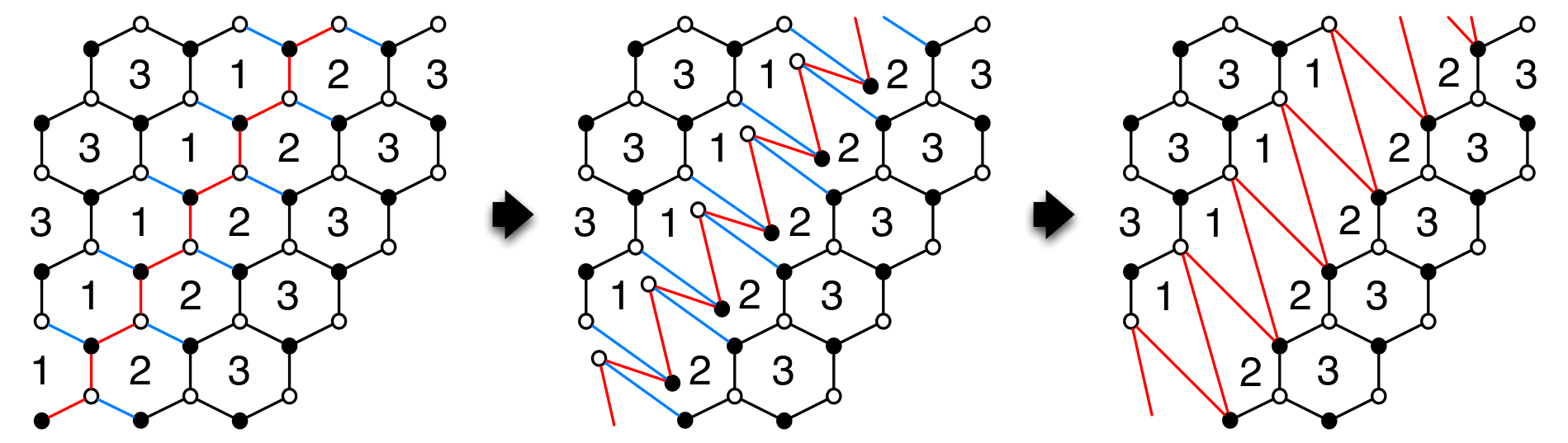
The mass deformation has effects on quivers, dimers and toric diagrams. In quivers, the arrows corresponding to fields which are integrated out are eliminated. On the dimer, the tiling is deformed taking away the integrated fields, reducing the number of edges in the corresponding faces/gauge groups. An example is shown in Fig. (6). On the toric diagram, external points are moved around the perimeter, but their number is preserved. Since the toric diagram changes, the mesonic moduli space changes as well.

This procedure connects different toric theories, such as $\mathbb{C}^{3}/\mathbb{Z}_{4}$ in Sec. (4.5) and the chiral orbifold of the Conifold $\mathcal{C}/{\mathbb{Z}}^{\prime}_{2}$ in Sec. (4.4), whose unoriented projections can thus be related.

The first prototypical example is the unoriented projection of $\mathbb{C}^{3}$ Franco:2007ii; Garcia-Etxebarria:2016bpb. The parent gauge theory is $\mathcal{N}=4$ Super Yang-Mills (SYM) theory with super-potential

where $\Phi_{I}$ are adjoint fields, which parametrize the three complex directions transverse to the stack of D3-branes. The toric diagram of this theory is a triangle with no internal point and consequently there are two different involutions given by an $\Omega 3$ or a non-compact $\Omega 7$.

Following the quiver description presented in Bianchi:2013gka, the orientifold charges for an $\Omega 3^{\pm}$, $(\pm,-,-,-)$ give $\mathcal{N}=4$ SYM with $Sp(SO)(N)$ gauge group and the three fields transforming in the (anti)symmetric representation; the orientifold charges for a $\Omega 7^{\pm}$, $(\mp,+,+,-)$ yield a $\mathcal{N}=2$ gauge theory with either $Sp(N)$ and two antisymmetric fields and one symmetric, or $SO(N)$ with two symmetric fields and one antisymmetric. The super-potential of the parent theory is easily read from the dimer and, after the unoriented projection, the product of the T-parities on the dimer must be negative due to the constraint given by Eq. (3.5). The first of various choices⁹⁹ 9 The first T-parity lays on the face, the other three follow in clockwise order on the dimer. is $(\tau_{0},\tau_{1},\tau_{2},\tau_{3})=(\mp,\pm,\pm,\pm)$, which gives $\mathcal{N}=4$ SYM. In fact, the three mesonic operators on the dimer flip their signs under $\Omega 3^{\pm}$. For this model the relation with the orientifold charges is $\epsilon_{0}=-\tau_{0}=\pm$, $\epsilon_{1}=\tau_{0}\tau_{1}=-$, $\epsilon_{2}=\tau_{0}\tau_{2}=-$, $\epsilon_{3}=\tau_{0}\tau_{3}=-$, and corresponds to an $\Omega 3^{\pm}$. On the other hand, the action of an $\Omega 7$ is encoded in such choices of T-parities as $(\pm,\pm,\pm,\mp)$ or permutation of the last three signs. The three diagrams are drawn in Fig. (7). Finally, note that $\Omega 3$ yields a conformally invariant theory with canonical dimensions and R-charges for the three adjoint chiral fields.

The next simplest case is a stack of regular D3-branes placed at the singularity $\mathbb{C}^{3}/\mathbb{Z}_{n}$. This gives a quiver theory with $n$ nodes, representing fractional branes wrapping internal cycles. Away from the origin, the space looks like $\mathbb{C}^{3}$, thus, moving the stack of D3 branes away of the singularity, the theory goes back to the conformal $\mathcal{N}=4$ SYM and the same reasoning holds with the unoriented projection $\Omega 3$ of an orbifold theory $\mathbb{C}^{3}/\mathbb{Z}_{n}$. This imposes that the beta functions $\beta_{a}$ add up to zero

which corresponds to a constant complex dilaton $S$. In fact, for $\mathbb{C}^{3}/\mathbb{Z}_{n}$ the gauge kinetic function at each node, $f_{a}$, sum up to $S$. Note that each node represent a stack of different kind of fractional D-branes: point-like D3’s, D5’s wrapped around 2-cycles and ‘compact’ D7’s wrapped around 4-cycles.

In this section we analyze the second prototypical example, the unoriented projection of the chiral orbifold $\mathbb{C}^{3}/\mathbb{Z}_{3}$ Feng_2001; Franco:2007ii; Garcia-Etxebarria:2016bpb, whose different descriptions are drawn in Fig. (8). We study the $\mathcal{N}=1$ theory with $k_{I}=(1,1,1)$, whose quiver is the same as the theory with $k_{I}=(2,2,2)$, up to relabelling the nodes. Among the conjugacy classes, summarized in Tab. (2), the single senior class signals the presence of a single compact 4-cycle and this information will be useful later.

The super-potential is

which enjoys the mesonic symmetry $SU(3)$. In fact, the theory has symmetry $SU(3)\times U(1)_{R}$, where $U(1)_{R}$ is the R-symmetry of the $\mathcal{N}=1$ SCFT.

Let us perform the unoriented projection with a compact $\Omega$7-plane in the resolved space, whose toric diagram is the left one showed in Fig. (8). Since $n=3$ is odd, there are only three equivalent projections with the $\Omega$-plane on top of a node. Here, without loss of generality, we consider only an $\Omega$-plane through the node 0. This orientifold involution acts on the orbifold as

and the super-potential becomes

The anomaly cancellation condition Eq. (3.9) reads

which is indeed what we would have obtained with an $\Omega 3^{\pm}$ placed at the origin of the singular space. According to the toric diagram, the orientifold plane is a compact $\Omega 7$ in the smooth resolved space, which wraps the compact 4-cycle (whose presence is signaled by the senior conjugacy class) that in the singular space corresponds to an $\Omega 3^{\pm}$-plane. The results are summarized in Tab. (3). From the dimer, we can reproduce this unoriented projection with four fixed points ${\tau}_{i}=(\pm,\mp,\mp,\mp)$ as displayed in Fig. (8) and negative overall product of the T-parities ${\tau}_{i}$. Again in this case, the relation between T-parities and orientifold charges is given by $\epsilon_{0}=-\tau_{0}$ and the relative sign of the mesonic operators under the orientifold involution $\epsilon_{I}=\tau_{0}\tau_{I}$.

Let us compute the $\beta$-functions. From Eq. (3.6) and using Eq. (4.6) we obtain

Assuming there is a conformal point, where $1-\gamma_{ab}=3(1-R_{ab})$, we have for the R-charges

where the last equation comes from the super-potential. The solution of the system is

from which $\gamma_{01}=-2\frac{\sum_{I=1}^{3}\epsilon_{11^{\prime}}^{(I)}}{N_{1}}$, $\gamma_{11^{\prime}}=+2\frac{\sum_{I=1}^{3}\epsilon_{11^{\prime}}^{(I)}}{N_{1}}$. Note that in the large $N$ limit we retrieve back the anomalous dimensions of the parent theory, namely, $\gamma_{11^{\prime}}=\gamma_{01}=0$ and the sum of the beta functions vanishes if $3\epsilon_{0}=\sum_{I=1}^{3}\epsilon_{11^{\prime}}^{(I)}$.

Note also that in the resolved space the compact $\Omega$7 acts in such a way that all the three fields $X_{11^{\prime}}^{I}$ are projected in the same way, as we can see from the anomaly cancellation condition Eq. (4.6).

References

- (1) M. Bianchi and A. Sagnotti, On the systematics of open string theories, Phys. Lett. B247 (1990) 517–524.
- (2) M. Bianchi and A. Sagnotti, Twist symmetry and open string Wilson lines, Nucl. Phys. B361 (1991) 519–538.
- (3) M. Bianchi, Open strings and dualities, J. Korean Phys. Soc. 33 (1998) S510–S519, [hep-th/9712020].
- (4) C. Angelantonj and A. Sagnotti, Open strings, Phys. Rept. 371 (2002) 1–150, [hep-th/0204089].
- (5) J. Dai, R. G. Leigh and J. Polchinski, New Connections Between String Theories, Mod. Phys. Lett. A4 (1989) 2073–2083.
- (6) J. Polchinski, Dirichlet Branes and Ramond-Ramond charges, Phys. Rev. Lett. 75 (1995) 4724–4727, [hep-th/9510017].
- (7) J. Polchinski, Tasi lectures on D-branes, in Fields, strings and duality. Proceedings, Summer School, Theoretical Advanced Study Institute in Elementary Particle Physics, TASI’96, Boulder, USA, June 2-28, 1996, pp. 293–356, 1996. hep-th/9611050.
- (8) J. M. Maldacena, The Large N limit of superconformal field theories and supergravity, Int. J. Theor. Phys. 38 (1999) 1113–1133, [hep-th/9711200].
- (9) E. Witten, Anti-de Sitter space and holography, Adv. Theor. Math. Phys. 2 (1998) 253–291, [hep-th/9802150].
- (10) S. S. Gubser, I. R. Klebanov and A. M. Polyakov, Gauge theory correlators from noncritical string theory, Phys. Lett. B428 (1998) 105–114, [hep-th/9802109].
- (11) O. Aharony, S. S. Gubser, J. M. Maldacena, H. Ooguri and Y. Oz, Large N field theories, string theory and gravity, Phys. Rept. 323 (2000) 183–386, [hep-th/9905111].
- (12) D. R. Morrison and M. R. Plesser, Nonspherical horizons. 1., Adv. Theor. Math. Phys. 3 (1999) 1–81, [hep-th/9810201].
- (13) S. Benvenuti, S. Franco, A. Hanany, D. Martelli and J. Sparks, An Infinite family of superconformal quiver gauge theories with Sasaki-Einstein duals, JHEP 06 (2005) 064, [hep-th/0411264].
- (14) D. Forcella, A. Hanany and A. Zaffaroni, Master Space, Hilbert Series and Seiberg Duality, JHEP 07 (2009) 018, [0810.4519].
- (15) O. Aharony, S. Kachru and E. Silverstein, New N=1 superconformal field theories in four-dimensions from D-brane probes, Nucl. Phys. B488 (1997) 159–176, [hep-th/9610205].
- (16) U. Bruzzo, A. Fino and P. Fré, The Kähler Quotient Resolution of Singularities, the McKay Correspondence and Chern–Simons Gauge Theories, Commun. Math. Phys. 365 (2019) 93–214, [1710.01046].
- (17) D. Martelli and J. Sparks, Toric geometry, Sasaki-Einstein manifolds and a new infinite class of AdS/CFT duals, Commun. Math. Phys. 262 (2006) 51–89, [hep-th/0411238].
- (18) S. Franco, A. Hanany, D. Martelli, J. Sparks, D. Vegh and B. Wecht, Gauge theories from toric geometry and brane tilings, JHEP 01 (2006) 128, [hep-th/0505211].
- (19) A. Hanany and R.-K. Seong, Brane Tilings and Reflexive Polygons, Fortsch. Phys. 60 (2012) 695–803, [1201.2614].
- (20) A. Hanany and R.-K. Seong, Brane Tilings and Specular Duality, JHEP 08 (2012) 107, [1206.2386].
- (21) S. Cremonesi, A. Hanany and R.-K. Seong, Double Handled Brane Tilings, JHEP 10 (2013) 001, [1305.3607].
- (22) S. Franco, A. Hanany, D. Krefl, J. Park, A. M. Uranga and D. Vegh, Dimers and orientifolds, JHEP 09 (2007) 075, [0707.0298].
- (23) I. Garcia-Etxebarria, B. Heidenreich and T. Wrase, New N=1 dualities from orientifold transitions. Part I. Field Theory, JHEP 10 (2013) 007, [1210.7799].
- (24) I. García-Etxebarria, B. Heidenreich and T. Wrase, New N=1 dualities from orientifold transitions - Part II: String Theory, JHEP 10 (2013) 006, [1307.1701].
- (25) I. García-Etxebarria and B. Heidenreich, Strongly coupled phases of S-duality, JHEP 09 (2015) 032, [1506.03090].
- (26) I. García-Etxebarria and B. Heidenreich, S-duality in 1 orientifold SCFTs, Fortsch. Phys. 65 (2017) 1700013, [1612.00853].
- (27) M. Bianchi, G. Inverso, J. F. Morales and D. Ricci Pacifici, Unoriented Quivers with Flavour, JHEP 01 (2014) 128, [1307.0466].
- (28) S. Franco and A. M. . Uranga, Dynamical SUSY breaking at meta-stable minima from D-branes at obstructed geometries, JHEP 06 (2006) 031, [hep-th/0604136].
- (29) S. Franco, Bipartite Field Theories: from D-Brane Probes to Scattering Amplitudes, JHEP 11 (2012) 141, [1207.0807].
- (30) S. Franco and A. Uranga, Bipartite Field Theories from D-Branes, JHEP 04 (2014) 161, [1306.6331].
- (31) S. Franco, E. García-Valdecasas and A. M. Uranga, Bipartite field theories and D-brane instantons, JHEP 11 (2018) 098, [1805.00011].
- (32) E. García-Valdecasas Tenreiro and A. Uranga, Backreacting D-brane instantons on branes at singularities, JHEP 08 (2017) 061, [1704.05888].
- (33) S. Franco, A. Retolaza and A. Uranga, D-brane Instantons as Gauge Instantons in Orientifolds of Chiral Quiver Theories, JHEP 11 (2015) 165, [1507.05330].
- (34) M. Billo, M. Frau, I. Pesando, F. Fucito, A. Lerda and A. Liccardo, Classical gauge instantons from open strings, JHEP 02 (2003) 045, [hep-th/0211250].
- (35) M. Billo, M. Frau, F. Fucito and A. Lerda, Instanton calculus in R-R background and the topological string, JHEP 11 (2006) 012, [hep-th/0606013].
- (36) M. Bianchi and E. Kiritsis, Non-perturbative and Flux superpotentials for Type I strings on the Z(3) orbifold, Nucl. Phys. B782 (2007) 26–50, [hep-th/0702015].
- (37) M. Bianchi, F. Fucito and J. F. Morales, D-brane instantons on the T**6 / Z(3) orientifold, JHEP 07 (2007) 038, [0704.0784].
- (38) M. Bianchi, F. Fucito and J. F. Morales, Dynamical supersymmetry breaking from unoriented D-brane instantons, JHEP 08 (2009) 040, [0904.2156].
- (39) R. Blumenhagen, M. Cvetic, S. Kachru and T. Weigand, D-Brane Instantons in Type II Orientifolds, Ann. Rev. Nucl. Part. Sci. 59 (2009) 269–296, [0902.3251].
- (40) M. Bianchi and G. Inverso, Unoriented D-brane instantons, Fortsch. Phys. 60 (2012) 822–834, [1202.6508].
- (41) U. Gursoy, E. Kiritsis and F. Nitti, Exploring improved holographic theories for QCD: Part II, JHEP 02 (2008) 019, [0707.1349].
- (42) U. Gursoy and E. Kiritsis, Exploring improved holographic theories for QCD: Part I, JHEP 02 (2008) 032, [0707.1324].
- (43) C. Angelantonj, M. Bianchi, G. Pradisi, A. Sagnotti and Ya. S. Stanev, Chiral asymmetry in four-dimensional open string vacua, Phys. Lett. B385 (1996) 96–102, [hep-th/9606169].
- (44) A. M. Uranga, The standard model in string theory from D-branes, Nucl. Phys. Proc. Suppl. 171 (2007) 119–138.
- (45) R. Blumenhagen, B. Kors, D. Lust and S. Stieberger, Four-dimensional String Compactifications with D-Branes, Orientifolds and Fluxes, Phys. Rept. 445 (2007) 1–193, [hep-th/0610327].
- (46) M. Berg, M. Haack and B. Kors, On the moduli dependence of nonperturbative superpotentials in brane inflation, in Themes in Unification. Proceedings: 10th International Symposium on particles, strings and cosmology, (PASCOS 2004), Pran Nath Festschrift. Part II: Boston, USA, August 18-19, 2004, 2004. hep-th/0409282.
- (47) M. Haack, R. Kallosh, A. Krause, A. D. Linde, D. Lust and M. Zagermann, Update of D3/D7-Brane Inflation on K3 x T**2/Z(2), Nucl. Phys. B806 (2009) 103–177, [0804.3961].
- (48) M. Bianchi, S. Cremonesi, A. Hanany, J. F. Morales, D. Ricci Pacifici and R.-K. Seong, Mass-deformed Brane Tilings, JHEP 10 (2014) 027, [1408.1957].
- (49) K. A. Intriligator and B. Wecht, The Exact superconformal R symmetry maximizes a, Nucl. Phys. B667 (2003) 183–200, [hep-th/0304128].
- (50) Y. Ito and M. Reid, The McKay correspondence for finite subgroups of SL(3,C), alg-geom/9411010.
- (51) R. Argurio and M. Bertolini, Orientifolds and duality cascades: confinement before the wall, JHEP 02 (2018) 149, [1711.08983].
- (52) I. R. Klebanov and M. J. Strassler, Supergravity and a confining gauge theory: Duality cascades and chi SB resolution of naked singularities, JHEP 08 (2000) 052, [hep-th/0007191].
- (53) N. Seiberg, Electric - magnetic duality in supersymmetric nonAbelian gauge theories, Nucl. Phys. B435 (1995) 129–146, [hep-th/9411149].
- (54) K. A. Intriligator and N. Seiberg, Lectures on supersymmetric gauge theories and electric-magnetic duality, Nucl. Phys. Proc. Suppl. 45BC (1996) 1–28, [hep-th/9509066].
- (55) V. Bouchard, Lectures on complex geometry, Calabi-Yau manifolds and toric geometry, hep-th/0702063.
- (56) U. Bruzzo, A. Fino, P. Fré, P. A. Grassi and D. Markushevich, Crepant resolutions of and the generalized Kronheimer construction (in view of the gauge/gravity correspondence), J. Geom. Phys. 145 (2019) 103467, [1902.01060].
- (57) S. Franco, A. Hanany, D. Vegh, B. Wecht and K. D. Kennaway, Brane Dimers and Quiver Gauge Theories, Journal of High Energy Physics 2006 (Jan, 2006) 096–096, [hep-th/0504110].
- (58) M. Yamazaki, Brane tilings and their applications, Fortschritte der Physik 56 (2008) 555–686, [0803.4474].
- (59) J. P. Gauntlett, D. Martelli, J. F. Sparks and D. Waldram, A New infinite class of Sasaki-Einstein manifolds, Adv. Theor. Math. Phys. 8 (2004) 987–1000, [hep-th/0403038].
- (60) M. Cvetic, H. Lu, D. N. Page and C. N. Pope, New Einstein-Sasaki spaces in five and higher dimensions, Phys. Rev. Lett. 95 (2005) 071101, [hep-th/0504225].
- (61) B. Feng, Y.-H. He, K. D. Kennaway and C. Vafa, Dimer models from mirror symmetry and quivering amoebae, Adv. Theor. Math. Phys. 12 (2008) 489–545, [hep-th/0511287].
- (62) Y. Imamura, K. Kimura and M. Yamazaki, Anomalies and O-plane charges in orientifolded brane tilings, JHEP 03 (2008) 058, [0801.3528].
- (63) M. Bianchi and J. F. Morales, Anomalies and tadpoles, Journal of High Energy Physics 2000 (2000) 030–030, [0002149].
- (64) G. Aldazabal, D. Badagnani, L. E. Ibáñez and A. M. Uranga, Tadpole versus anomaly cancellation in d = 4,6 compact iib orientifolds, Journal of High Energy Physics 1999 (1999) 031–031, [9904071].
- (65) I. R. Klebanov and E. Witten, Superconformal field theory on three-branes at a Calabi-Yau singularity, Nucl. Phys. B536 (1998) 199–218, [hep-th/9807080].
- (66) B. Feng, A. Hanany and Y. He, Phase structure of d-brane gauge theories and toric duality, Journal of High Energy Physics 2001 (Aug, 2001) 040–040, [hep-th/0104259].
- (67) B. Feng, S. Franco, A. Hanany and Y.-H. He, UnHiggsing the del Pezzo, JHEP 08 (2003) 058, [hep-th/0209228].
- (68) M. Bertolini, F. Bigazzi and A. L. Cotrone, New checks and subtleties for AdS/CFT and a-maximization, JHEP 12 (2004) 024, [hep-th/0411249].
- (69) D. Berenstein, C. P. Herzog, P. Ouyang and S. Pinansky, Supersymmetry breaking from a Calabi-Yau singularity, JHEP 09 (2005) 084, [hep-th/0505029].
- (70) M. Bertolini, F. Bigazzi and A. L. Cotrone, Supersymmetry breaking at the end of a cascade of Seiberg dualities, Phys. Rev. D72 (2005) 061902, [hep-th/0505055].
- (71) M. Bianchi, F. Fucito, G. Rossi and M. Martellini, On the ADHM construction on ALE gravitational backgrounds, Phys. Lett. B 359 (1995) 49–55.
- (72) M. Bianchi, F. Fucito, G. Rossi and M. Martellini, Explicit construction of Yang-Mills instantons on ALE spaces, Nucl. Phys. B 473 (1996) 367–404, [hep-th/9601162].
- (73) A. Lawrence, N. Nekrasov and C. Vafa, On conformal field theories in four dimensions, Nuclear Physics B 533 (Nov, 1998) 199–209, [hep-th/9803015].
- (74) A. Hanany and Y.-H. He, Non-abelian finite gauge theories, Journal of High Energy Physics 1999 (Feb, 1999) 013–013, [hep-th/9811183].
- (75) J. Park, R. Rabadan and A. M. Uranga, Orientifolding the conifold, Nucl. Phys. B570 (2000) 38–80, [hep-th/9907086].
- (76) D. Forcella, A. Hanany and A. Zaffaroni, Master space, hilbert series and seiberg duality, Journal of High Energy Physics 2009 (Jul, 2009) 018–018, [hep-th/0810.4519].
- (77) K. A. Intriligator and P. Pouliot, Exact superpotentials, quantum vacua and duality in supersymmetric SP(N(c)) gauge theories, Phys. Lett. B353 (1995) 471–476, [hep-th/9505006].
- (78) K. A. Intriligator and N. Seiberg, Duality, monopoles, dyons, confinement and oblique confinement in supersymmetric SO(N(c)) gauge theories, Nucl. Phys. B444 (1995) 125–160, [hep-th/9503179].
- (79) A. M. Uranga, Brane configurations for branes at conifolds, JHEP 01 (1999) 022, [hep-th/9811004].
- (80) R. Argurio, M. Bertolini, G. Ferretti, C. Petersson and A. Lerda, Stringy instantons at orbifold singularities, Journal of High Energy Physics 2007 (2007) 067–067, [hep-th/0704.0262].
- (81) R. Argurio, M. Bertolini, S. Meynet and A. Pasternak, On supersymmetry breaking vacua from d-branes at orientifold singularities, Journal of High Energy Physics 2019 (2019) , [hep-th/1909.04682].