Chiral SO(4) spin-valley density wave and degenerate topological superconductivity in magic-angle-twisted bilayer-graphene
Abstract
Starting from a realistic extended Hubbard model for a -orbital tight-binding model on the Honeycomb lattice, we perform a thorough investigation on the possible electron instabilities in the magic-angle-twisted bilayer-graphene near the van Hove (VH) dopings. Here we focus on the interplay between the two symmetries of the system. One is the approximate SU(2)SU(2) symmetry which leads to the degeneracy between the inter-valley spin density wave (SDW) and valley density wave (VDW) as well as that between the inter-valley singlet and triplet superconductivities (SCs). The other is the symmetry which leads to the degeneracy among the three symmetry-related wave vectors of the density-wave (DW) orders, originating from the Fermi-surface nesting. The interplay between these two degeneracies leads to intriguing quantum states relevant to recent experiments, as revealed by our systematic random-phase-approximation based calculations followed by a succeeding mean-field energy minimization for the ground state energy. At the SU(2)SU(2) symmetric point, the degenerate inter-valley SDW and VDW are mixed into a new state of matter dubbed as the chiral SO(4) spin-valley DW. This state simultaneously hosts three 4-component vectorial spin-valley DW orders with each adopting one wave vector, and the polarization directions of the three DW orders are mutually perpendicular to one another. In the presence of a tiny inter-valley exchange interaction with coefficient which breaks the SU(2)SU(2) symmetry, a pure chiral SDW state is obtained. In the case of , although a nematic VDW order is favored, the two SDW orders with equal amplitudes are accompanied simultaneously. This nematic VDW+SDW state possesses a stripy distribution of the charge density, consistent with the recent STM observations. On the aspect of SC, while the triplet and singlet topological SCs are degenerate at near the VH dopings, the former (latter) is favored for (). In addition, the two asymmetric doping-dependent behaviors of the obtained pairing phase diagram are well consistent with experiments.
I Introduction
The condensed-matter community is witnessing a surge in the synthesis and research of novel graphene-multi-layer-heterostructure materials Cao et al. 2018a; Cao et al. 2018b; Cao et al. 2019; Choi et al. 2019; Jiang et al. 2019; Kerelsky et al. 2019; Liu et al. 2019a; Shen et al. 2019; Chen et al. 2019a; Chen et al. 2019b; Chen et al. 2020; Yankowitz et al. 2019; Xie et al. 2019 with Moiré pattern superstructure Bistritzer and MacDonald 2011; Dos Santos et al. 2007; Chittari et al. 2019; Wu et al. 2018a; Xian et al. 2019; Tomarken et al. 2019; Da Liao et al. 2019; Hu et al. 2019; Yudhistira et al. 2019; Padhi and Phillips 2019; Ramires and Lado 2019; Schrade and Fu 2019; Bi et al. 2019; Lin and Nandkishore 2019; Klebl and Honerkamp 2019; Pizarro et al. 2019a; Goodwin et al. 2019a, leading to the greatly enlarged unit cell and hence thousands of energy bands within the Moiré Brillouin zone (MBZ). Remarkably, several isolated flat bands emerge within the high-energy band gap, which brings about strong electron correlations and different types of electronic instabilities, including the correlated insulators and superconductivity (SC). Here we focus on the magic-angle-twisted bilayer-graphene (MA-TBG) Cao et al. 2018a; Cao et al. 2018b, in which spin-unpolarized Yankowitz et al. 2019 correlated insulating phases are revealed when the low energy flat valence or conduction bands are half-filled, and it leads to the novel SC after doping.
Currently, the characterization of the correlated insulating phase near this doping level Zhu et al. 2019; Wu et al. 2019a; Goodwin et al. 2019b; Cao et al. 2018b; Venderbos and Fernandes 2018; Haule et al. 2019; Kang and Vafek 2018; Kang and Vafek 2019; Xu et al. 2018; Padhi et al. 2018; Pizarro et al. 2019b; Thomson et al. 2018; Zhang et al. 2019a; Liu et al. 2019b; Xie and MacDonald 2020; Wu et al. 2019b; Yuan and Fu 2018; Codecido et al. 2019; Dodaro et al. 2018; Liu et al. 2018; Fidrysiak et al. 2018; Guo et al. 2018; Ochi et al. 2018; Lu et al. 2019; Huang et al. 2019; Rademaker and Mellado 2018; Classen et al. 2019; Kennes et al. 2018; Isobe et al. 2018; Sherkunov and Betouras 2018; Bultinck et al. 2020; Kang and Vafek 2020; Zhang et al. 2020a; Soejima et al. 2020; Xie et al. 2021, the pairing mechanism, and pairing symmetry Cao et al. 2018a; Codecido et al. 2019; Dodaro et al. 2018; Liu et al. 2018; Fidrysiak et al. 2018; Guo et al. 2018; Classen et al. 2019; Kennes et al. 2018; Ochi et al. 2018; Isobe et al. 2018; Lu et al. 2019; Huang et al. 2019; Rademaker and Mellado 2018; Sherkunov and Betouras 2018; Xu and Balents 2018; Roy and Juričić 2019; Zhang 2019; Ray et al. 2019; Su and Lin 2018; Peltonen et al. 2018; Wu et al. 2018b; Lian et al. 2019; Zhang et al. 2020b; Brydon et al. 2019; Angeli et al. 2019; Tang et al. 2019; Alidoust et al. 2019; Wu 2019; Wu and Sarma 2019; Wang et al. 2019; Chen et al. 2018; Liu et al. 2019c; Choi and Choi 2018; You and Vishwanath 2019; Gonzalez and Stauber 2019; Laksono et al. 2018; Wu et al. 2019c; Fang et al. 2019; Wu et al. 2019d; Chichinadze et al. 2019 are still under debate. Particularly, two opposite points of view are held, i.e. the strong-coupling Mott-insulating picture and the weak-coupling itinerant picture. Here we start from the weak-coupling viewpoint first proposed in Ref. Liu et al. 2018 that the correlated insulator and SC in the MA-TBG are driven by Fermi-surface (FS) nesting near the van Hove singularity (VHS) Isobe et al. 2018; You and Vishwanath 2019; Lin and Nandkishore 2018; Gonzalez and Stauber 2019; Laksono et al. 2018; Sherkunov and Betouras 2018; Kennes et al. 2018; Kozii et al. 2019; Yuan et al. 2019; Classen et al. 2019; Wu et al. 2021; Cea et al. 2019; Rademaker et al. 2019; Harshman and Fiory 2020. The key point is that the spin or charge susceptibility would diverge as the system is doped to the VHS point with good FS-nesting, leading to the spin or charge (including valley) density wave (DW). When the doping level deviates from the DW ordered regime, the short-ranged DW fluctuations would mediate the SC. Two questions naturally arise: What type of spin or/and charge (or valley) DW would be driven by the FS-nesting near the VHS for the MA-TBG? What is the pairing symmetry mediated by the DW fluctuations?
The answers of the two questions are deeply related to the symmetries of the MA-TBG. One relevant symmetry is the symmetry. In the weak-coupling theories Liu et al. 2018; Isobe et al. 2018; You and Vishwanath 2019, the wave vector of the DW orders is determined by the FS-nesting vector. However, the presence of the symmetry brings about three degenerate FS-nesting vectors Liu et al. 2018; Isobe et al. 2018; You and Vishwanath 2019. The different DW orders hosting these degenerate wave vectors can be mixed to minimize the energy in general, leading to an exotic ground state. For example, in the theory proposed in Ref. Liu et al. 2018, the three SDW orders hosting degenerate wave vectors of and would coexist and be equally mixed into the chiral SDW state, in which the polarization directions of the three vectorial SDW order parameters are mutually perpendicular and can be globally arbitrarily rotated in the space by the Goldstone zero modes. This state breaks the time-reversal symmetry (TRS), and can be topologically nontrivial with nonzero Chern numbers.
The other relevant symmetry is associated with the special valley degree of freedom of the MA-TBG. As revealed in the continuum-theory model Wu et al. 2018b, the electron states within the two different MBZs centered at and would not hybridize for small twist angles, leading to two isolated and TR related sectors of energy bands, leading to the valley-U(1) symmetry, which survives the electron-electron interactions Yuan and Fu 2018; Po et al. 2018; Kang and Vafek 2018; Isobe et al. 2018; Ochi et al. 2018; You and Vishwanath 2019; Koshino et al. 2018; Po et al. 2019. Besides, this system additionally holds a spin SU(2)SU(2) symmetry Isobe et al. 2018; You and Vishwanath 2019. Although this symmetry survives the dominant interactions in the MA-TBG, it would be slightly broken by a tiny inter-valley exchange interaction whose strength is much lower than any other energy scale of the system and can be treated as . The SU(2)SU(2) symmetry has a profound influence on the formula of the order parameters of the instabilities of the MA-TBG: it leads to the degeneracy between the inter-valley spin DW (SDW) and valley DW (VDW) as well as that between the inter-valley-pairing spin-singlet and spin-triplet SCs of the MA-TBG Isobe et al. 2018; You and Vishwanath 2019. Due to these degeneracies at the exactly-symmetric point, it’sit is generally perceived that the realized instabilities in the MA-TBG are determined by the tiny : for the case of (), a pure SDW (VDW) will be the realized DW order, and a triplet (singlet ) will be the pairing symmetry Isobe et al. 2018; You and Vishwanath 2019. However, here we hold a different point of view, as introduced below.
The fact that the SDW and VDW orders are degenerate at the exactly SU(2)SU(2)-symmetric point with doesn’t necessitate that only one of them is the candidate for a tiny . Actually, the two orders can generally be mixed to lower the ground-state energy in any case. The right procedure for the identification of the ground-state DW orders for different is as follow. Firstly, we should identify the energetically minimized mixing manner between the SDW and VDW at the symmetric point with . Note that the mixing manner thus obtained is not unique, as the spontaneous breaking of the SU(2)SU(2) symmetry always leads to gapless Goldstone modes which can rotate one ground state to numerous other degenerate ones, forming a ground-state subspace. Then the realistic tiny -term sets in, which serves as a perturbative symmetry-breaking field and will select its favorite states from this subspace. These states form the ground states for nonzero . Note that the symmetry plays an important role in this procedure: it will introduce three times as many states to participate in the mixing, which fundamentally changes the ground state. The ground state thus obtained turns out to be fundamentally different from the intuitively conjectured one in Ref. Isobe et al. 2018; You and Vishwanath 2019.
In this paper, we perform a thorough investigation on the DW orders and SC in the MA-TBG driven by FS-nesting near the VHS, with a particular attention paid to the interplay between the approximate SU(2)SU(2) symmetry and the threefold degeneracy among the wave vectors of the DW orders. Through adopting realistic band structure and interaction terms that respect all symmetries of the system, we carry out systematic calculations based on the random-phase approximation (RPA) and subsequent mean-field (MF) energy minimization for the ground state. We have also provided a phenomenological Ginzburg-Landau theory to account for our microscopic results. While the RPA calculations suggest that the critical interactions and for the SDW and VDW orders are equal at , the subsequent MF energy minimization yields that the SDW ground state holds a lower energy because its vectorial order parameters allow three times as many states to participate in the mixing and thus have more opportunity to lower the energy. When we further allow the SDW and VDW to mix, a novel chiral SO(4) spin-valley DW state with exotic properties is obtained, as will be introduced in Sec. II. When the tiny inter-valley exchange interaction term is added, we obtain the pure chiral SDW state for and a nematic DW state with mixed SDW and stripy VDW orders for . The latter case is consistent with the recent STM experiment Jiang et al. 2019; Kerelsky et al. 2019, and might be more probably realized in the MA-TBG. On the -dependent pairing symmetries, our results are essentially consistent with the intuitively conjectured one in Ref. Isobe et al. 2018; You and Vishwanath 2019.
The rest of this paper is organized as follows. Section II provides an overview on the main results provided in this work. In Sec. III, we describe the model and the approach. A two-orbital tight-binding (TB) model on the honeycomb lattice is provided, added with realistic interaction terms. The RPA approach and the subsequent MF analysis are introduced. In Sec. IV, we study the case of , in which the system hosts the exact SU(2)SU(2) symmetry. The degeneracies between the SDW and VDW as well as between the singlet and triplet SCs are analyzed in detail. We find that the SDW and VDW can mix into the chiral SO(4) spin-valley DW. In Sec. V, we provide our results for the cases with tiny , including and . These two cases have different DW states and pairing symmetries. Finally, a conclusion will be reached with some discussions in Sec. VI.
II Overview
This section provides an overview on the present work, which is focused on how the interplay between the approximate SU(2)SU(2) symmetry and the symmetry will influence the formula of the order parameters of the DW and SC in the MA-TBG. Briefly speaking, our answer to the question about the DW is fundamentally different from the generally perceived one. Due to the degeneracy between the SDW and VDW and that between singlet and triplet pairings at the exact SU(2)SU(2)-symmetric point with , it’sit is generally intuitively perceived that for the case of (), a pure SDW (VDW) will be realized, and a triplet (singlet ) will be the pairing symmetry Isobe et al. 2018; You and Vishwanath 2019. However, here we propose that the two DW orders are generally mixed. In the case of , we obtained the chiral SO(4) spin-valley DW, which evolves into a pure chiral SDW upon and a nematic DW with mixed SDW and stripy VDW orders upon . The latter case is consistent with recent STM observations. For the SC, our answer is consistent with the generally perceived viewpoint.
Our start point is the -orbital tight-binding (TB) model on the Honeycomb lattice Yuan and Fu 2018; Koshino et al. 2018, equipped with realistic extended Hubbard interactions including a tiny inter-valley exchange interaction. While the TB part and the dominant interactions in this Hamiltonian possess the SU(2)SU(2) symmetry, which is broken by the tiny inter-valley exchange interaction. Besides, the model holds a symmetry, which leads to three degenerate FS-nesting vectors near the VHS points. In our calculations, we first carry out systematic RPA based studies to figure out the forms of all possible instabilities, and then perform a subsequent MF energy minimizations to pin down the mixing manner between degenerate orders. Finally, in order to account for the results obtained by our microscopic calculations, we have also provided a phenomenological Ginzburg-Landau theory to classify all the possible configurations of the DW order parameters, which emerge as possible solutions to minimize the G-L free energy function. Our results are summarized in Fig. 1.
The results for the case of are listed in the row of in Fig. 1(a). In this case, the critical interactions and for the SDW and VDW orders are equal, and the leading spin-singlet () and spin-triplet () pairings have equal . The degeneracy between the SDW and VDW makes them mix into the chiral SO(4) spin-valley DW ordered state. This DW state is characterized by three coexisting four-component vectorial order parameters () shown in Fig. 1(b), with each hosting one wave vector . Here, and represent the SDW and VDW order parameters hosting the wave vector , respectively. The three 4-component vectorial order parameters are mutually perpendicular to one another, i.e. , and can be globally arbitrarily rotated in the order-parameter space by the Goldstone zero modes, as shown in Fig. 1(b). This phase is a generalization of the 3Q chiral SDW state proposed previously Liu et al. 2018; Li 2012; Martin and Batista 2008; Kato et al. 2010; Jiang et al. 2014 to the VDW-SDW order-parameter space, and represents a new state of matter that possesses a series of intriguing properties. For example, this DW ground state hosts seven branches of gapless Goldstone modes. In addition, the topological properties of this DW state can be nontrivial with nonzero Chern number, as long as a DW gap opens at the Fermi level.
The results for (Hund-like) are listed in the row of in Fig. 1(a). In this case, our RPA calculation yields , suggesting that the SDW is preferred to the VDW. Therefore, in the VDW-SDW order-parameter space, the VDW axis becomes the “difficult” axis and would be kicked out from the low-energy degree of freedom. As a result, our subsequent MF energy minimization yields the pure 3Q chiral SDW state characterized as , with , as shown in Fig. 1(c). This state is qualitatively the same as that obtained previously Liu et al. 2018; Li 2012; Martin and Batista 2008; Kato et al. 2010; Jiang et al. 2014, which hosts four branches of gapless Goldstone modes one. The Chern number can also be nonzero, as long as an SDW gap opens at the Fermi level. As for the SC, the triplet SC with pairing symmetry is preferred.
The results for (anti-Hund-like) are listed in the row of in Fig. 1(a). In this case, our RPA calculation yields , suggesting that the VDW is preferred to the SDW. Therefore, in the VDW-SDW order-parameter space, the VDW axis becomes the “easy” axis. However, this doesn’t suggest a pure VDW state as generally perceived Isobe et al. 2018; You and Vishwanath 2019, because here we have three 4-component vectorial DW order parameters, which can not all point along the “easy” VDW axis, as their mutual perpendicular relation is robust against the tiny term. Our subsequent MF energy minimization yields a DW state with one scalar VDW component mixed with two mutually perpendicular vectorial SDW components with equal amplitude, with the VDW randomly choosing one wave vector from the three symmetry-related ones and the two SDW hosting the remaining two. Obviously, this nematic DW state spontaneously breaks the rotation symmetry, and the obtained stripy charge order is consistent with recent STM experiments Jiang et al. 2019; Kerelsky et al. 2019. This DW state is schematically shown in Fig. 1(d). The number of Goldstone modes and the topological properties in this case are the same as those in . As for the SC, the singlet SC with pairing symmetry is preferred.
The schematic phase diagram with respect to the - parameters are shown in Fig. 1(e). Besides the -dependence, our results reveal two asymmetric doping-dependent behaviors in the pairing phase diagram. One is the asymmetry with respect to the charge neutral point (CNP): the at the negative dopings is much higher than that at the positive dopings, which is due to the higher DOS in the former case. The other asymmetry is with respect to each VH doping: the on the higher-doping side of each VH point is higher than that on its lower-doping side. This asymmetry is attributed to the better FS-nesting and hence stronger DW fluctuations in the former case. These two asymmetric doping-dependent behaviors are well consistent with the experiments Cao et al. 2018a; Yankowitz et al. 2019, implying that the pairing in the MA-TBG should be mediated by the spin-valley DW fluctuations.
III Model and Approach

III.1 Model
For the MA-TBG there are four low-energy flat bands that are well isolated from the high-energy bandsNam and Koshino 2017; Moon and Koshino 2012; Fang and Kaxiras 2016; Dos Santos et al. 2007; Dos Santos et al. 2012; Shallcross et al. 2008; Bistritzer and MacDonald 2011; Bistritzer and MacDonald 2010; Uchida et al. 2014; Mele 2011; Mele 2010; Sboychakov et al. 2015; Morell et al. 2010; Trambly de Laissardière et al. 2010; Latil et al. 2007; De Laissardière et al. 2012; Huang et al. 2018; Guinea and Walet 2019; Gonzalez 2013; Gonzalez-Arraga et al. 2017; Cao et al. 2016; Ohta et al. 2012; Kim et al. 2017; Huder et al. 2018; Li et al. 2017; Zhang et al. 2019a; Yuan and Fu 2018; Song et al. 2019; Hejazi et al. 2019; Po et al. 2018; Zhang 2019; Ray et al. 2019; You and Vishwanath 2019; Kang and Vafek 2018; Koshino et al. 2018; Pal 2018; Guinea and Walet 2018; Zou et al. 2018; Po et al. 2019; Tarnopolsky et al. 2019; Ahn et al. 2019; Morell et al. 2010; De Laissardière et al. 2012; Chebrolu et al. 2019. The four flat bands can be divided into two valence bands and two conduction bands, which touch at the charge neutral point (CNP), i.e., and points in the MBZ. Besides the four-fold degeneracy at the CNP, the valence and conduction bands each are two-fold degenerate along the and lines. The continuum theory Bistritzer and MacDonald 2011; Bistritzer and MacDonald 2010 tells that these degeneracies are the consequence of the so-called U(1)-valley symmetry of the TBG with small twist angles. This symmetry forbids the hopping from the MBZ in the valley to that in the valley. While the TB models in Ref. Po et al. 2019 can faithfully describe the low-energy flat bands in both aspects of the symmetry and the topology at the CNPs, they are too complicated to be sufficiently convenient for succeeding studies with electron-electron interactions. Here we focus on the low-energy band structure near the Fermi level for the doped case, particularly near the VHS points which are related to experiments, which allows us to adopt simpler band structures.
The proposed simplest TB model for the MA-TBG is that on the honeycomb lattice containing a - and a -orbitals on each site Yuan and Fu 2018; Po et al. 2018; Kang and Vafek 2018; Liu et al. 2018; Koshino et al. 2018, with the orbitals on adjacent cites coupling via coexisting - and - bondings Liu et al. 2018. It’s proved in Appendix A that the valley-U(1) symmetry requires that the amplitudes of the - and - bondings are equal. In such a condition, we transform the -representation into the valley representation by , where is the annihilation operator of the electron on the -th site with spin and orbital ( represents the or orbital) and represent the and valleys. Consequently, we can find the following TB Hamiltonian Yuan and Fu 2018; Koshino et al. 2018,
| (1) |
More details are provided in Appendix A. Here, is the annihilation operator of the electron with the band index , the valley index , the wave vector and the spin . The energy is with respect to the chemical potential . denotes the -th neighboring bond. is the hopping strength that is caused by the and bonding Wu and Sarma 2008; Wu 2008; Zhang et al. 2014; Liu et al. 2014; Yang et al. 2015 and is responsible for the Kane-Mele type of the valley-orbital coupling Yuan and Fu 2018; Koshino et al. 2018. In our calculations, we consider up to the third-neighbor hoppings, i.e. . The chemical potential is determined by the doping with respect to the CNP. is the average electron number per unit cell with for the CNP.
The TB model in Eq. (III.1) tells that the and valley bands are separated with each other, leading to a valley-U(1) symmetry. Moreover, each valley independently supports the spin-SU(2) symmetry, leading to an SU(2)SU(2) symmetry. Finally, the geometry of the TBG leads to a point group. Figure 2(a) shows the corresponding band structure with the TB parameters provided in the figure caption. As a result of the U(1)-valley symmetry, points are four-fold degenerate, and and points are doubly degenerate. The U(1)-valley symmetry is also responsible for the double degeneration of the and lines. These characters are consistent with the continuum theory. The hump and dip in the two middle bands along the line give two VHS points for the hole and electron dopings respectively, see Fig. 2(b). They, denoted as the h-VHS and e-VHS, are both near the points and correspond to the doping of -0.182 and 0.240, respectively. These two VHSs originate from the the Lifshitz transition points, which can be seen from the FSs in Figs. 2(c) and 2(d). The valley-separated FSs reflect the inter-valley nesting behavior whose three nesting vectors are marked as (). These nesting vectors do not exactly connect the points, different from the previous model in Ref. Liu et al. 2018.
Note that in the Supplementary Material SM, we provide the FSs at the e-VH and h-VH dopings for five different twist angles near the magic angle, which is 1∘, 1.05∘, 1.1∘, 1.15∘ and 1.2∘. The band structure is obtained via the continuum modelBistritzer and MacDonald 2011. The resulting FSs clearly exhibit the presence of the Lifshitz transitions, which leads to the VHSs. What’s more, in these FSs there are also approximate FS nesting with three-folded rotation symmetry related nesting vectors () whose exact values depend on the twist angles.
Symmetry analysis and the extended character of the Wannier bases Po et al. 2018; Koshino et al. 2018; Ochi et al. 2018 suggest the following interaction terms for the MA-TBG,
| (2) |
where , , and . The extended density-density interactions between neighboring sites are represented by the terms which are up to the third neighbor. The relation among and is assumed to be Ochi et al. 2018; Koshino et al. 2018. The exchange interaction is taken according to Ref. Koshino et al. 2018. The tiny inter-valley Hund’s-rule exchange interaction is given by the last term with the coefficient two orders of magnitude weaker than Lee et al. 2019, and the parameters , and satisfy the relation .
The model (III.1) provides a realistic description for the electron-electron interactions in the MA-TBG. The total Hamiltonian of the system is given by
| (3) |
Note that all the terms except the tiny term conserve the SU(2)SU(2) symmetry, which is broken by the tiny term to the valley-U(1) symmetry plus the global spin-SU(2) symmetry. In our study, we considered the three different cases, i.e. , and , for comparison. As will be seen below, the three different cases will lead to qualitatively different ground states. In realistic material, the interaction strength is estimated to be comparable with the band widthCao et al. 2018a. Although in some studyKang and Vafek 2019 the is estimated to be about an order of magnitude larger than that adopted here, the band width of the MA-TBG measured by the STMXie et al. 2019 is also an order of magnitude larger than that adopted here. The experimentally-measured bandwidth can be viewed as that renormalizd by electron-electron interaction, and our TB band structure can also be viewed as the one renormalized by interaction. Therefore, our model can be viewed as rescaled from the realistic material by a factor of about 10. Such rescaling will not alter the qualitative behavior of the system
III.2 The RPAMF approach
The RPA approach is used in this work to identify the electron instabilities driven by the FS-nesting and VHS. According to the standard multi-orbital RPA approach Takimoto et al. 2004; Yada and Kontani 2005; Kubo 2007; Kuroki et al. 2008; Graser et al. 2009; Maier et al. 2011; Liu et al. 2013; Wu et al. 2014; Ma et al. 2014; Zhang et al. 2015, the following bare susceptibility is defined for the non-interacting case, namely,
| (4) |
where and are the wave vectors and with A and B representing the sublattice index and denoting the and valleys respectively. The denotes the thermal average of the noninteracting system. The explicit formula of is given in the Appendix B.
When interactions turn on, we define the following renormalized spin and charge susceptibilities,
| (5a) | ||||
| (5b) | ||||
In the RPA level, they are related to the bare susceptibility through the relation
| (6a) | ||||
| (6b) | ||||
Here, are the Fourier transformations of in the imaginary-frequency space, which are operated as matrices by taking the upper and lower two indices as one number, respectively. Note that we only provide the -component of the spin susceptibility. In the presence of spin-SU(2) symmetry, the other two components, i.e. the and components are equal to the component. The forms for are given in Appendix B.
If , the denominator matrix in Eq. (6a) (Eq. (6b)) has zero eigenvalue(s) for some and the renormalized zero-frequency spin (charge) susceptibility diverges, implying the formation of DW order in the spin (charge) channel. The concrete formulism of the interaction-induced DW order in the spin (charge) channel can be constructed as follow.
Let () from below, get the eigenvector corresponding to the largest eigenvalue of . Here the momentum , at which first diverges, provides the wave vector of the interaction-induced magnetic (valley) order, and the eigenvector () provides the form factor of the induced order. Generally in the weak-coupling limit, the wave vector of the interaction-induced order is equal to the FS-nesting vector. Due to the three-folded rotational symmetry of the system, there exist three degenerate FS-nesting vectors with , and so do the wave vectors of the induced order. As a result, the interaction-induced SDW or CDW order can be described by the following order-parameter part of the Hamiltonian,
| (7) |
Here is the vectorial Pauli matrix , and is the global amplitude of the -th vectorial SDW (scalar CDW) order parameter determined by the interaction strength via the following MF energy minimization.
Firstly, let’s write down the total MF- Hamiltonians describing the two ordered phases
| (8a) | ||||
| (8b) | ||||
After diagonalizing the two Hamiltonians, we obtain their ground states and . Secondly, the two MF energies are represented by the expectation values of the original Hamiltonian (3) in the two ground states, i.e.,
| (9a) | ||||
| (9b) | ||||
Note that the Wick’s decomposition procedure is adopted in calculating the above two expectation values. Finally, tuning the SDW or CDW order parameters or so that the above two MF- energies are minimized, after which we obtain these order parameters.
An important property of the DW orders obtained at slightly larger than is that they are either intra-valley orders or inter-valley ones, but not their mixing. To clarify this point, we put aside the sublattice and spin indices of or defined in Eq. (5) and only focus on the valley degree of freedom, which leads to
| (10) |
with the valley index denoting and valleys, respectively. Since the valley-U(1) symmetry of the system requires the conservation of the total value of valleys, i.e. , should take the form of
| (11) |
Here the correspondence between the value of or and the row or column index is . Due to the block-diagonalized character of the matrices shown in Eq. (11), any of their eigenvectors can either take the form of or of . While the form represents the intra-valley order, the latter denotes the inter-valley one, which do not mix. Note that the FS-nesting vectors shown in Fig. 2(c) and (d) always connect the FSs from different valleys, we can easily conjecture that the induced DW orders are inter-valley orders, which is consistent with our following calculation results.
Note that although the DW order obtained in the charge channel breaks the translational symmetry, the distribution of the charge density in this state is actually translational invariant due to its inter-valley coherence character. Therefore, it’sit is inappropriate to name this state as CDW. Instead, it should better be dubbed as the valley DW (VDW), as it breaks the valley-U(1) symmetry. In the following, we rename such quantity as , and to be , and . The DW order obtained in the spin channel breaks the translational symmetry, the spin-SU(2) and valley-U(1) symmetry. Therefore, we should better name it as valley-spin DW. In the following, we simply dub it as SDW for convenience.
When both and are satisfied, an effective pairing interaction vertex is developed through exchanging the short-ranged spin (charge) fluctuations between a Cooper pair. The detailed expression of is provided in the Appendix B. It leads to the following linearized gap equation near the superconducting critical temperature ,
| (12) |
where and label the bands that cross the FS, corresponding to combined in Eq. (III.1). gives the Fermi velocity and is the tangent component of along the FS. After discretization, the equation (12) presents as an eigenvalue problem. The eigenvector represents the gap form factor and the eigenvalue determines the through . Symmetry analysis requires that each is attributed to one of the three irreducible representations of the point group . Further considering the parity of in the absence of spin-orbit-coupling, there are six possible pairing symmetries Liu et al. 2018, i.e., , , and pairings for the spin singlet and , , and pairings for the spin triplet.
Since the superconducting critical temperature is much lower than the total band width of the low-energy emergent flat bands, it is reasonable to only consider the weak-pairing limit, in which only the electrons on the FS participate in the pairing. In such a condition, the Anderson’s theorem requires that the Cooper pairing can only take place between inter-valley. Moreover, these inter-valley pairings are neither valley-singlet pairing nor valley-triplet one, but instead are a mixing between them, as the square of the total vectorial valley of the Cooper pair is not a good quantum number here. Actually, if an electron with momentum-valley - is on the FS and thus can participate in the pairing, the electron with momentum-valley - is generally away from the FS and thus cannot participate in the pairing, which leads to a ratio of 1:0 between the amplitudes for the parings of and , leading to a 1:1 mixing between the valley-singlet and valley-triplet pairings.
IV Chiral SO(4)-DW and degenerate SC at
As introduced in Sec. III.1, when the inter-valley Hund’s coupling is neglected, the MA-TBG has an SU(2)SU(2) symmetry, with each valley independently hosting a spin-SU(2) symmetry. In this section, we will explore the consequence of such a symmetry. It will be seen below that degeneracies will take place either between the SDW and VDW or between the singlet and triplet SCs. The degeneracy between the SDW and VDW orders, in combination with the three-folded degeneracy among the wave vectors of the DW orders caused by the point group of the MA-TBG, would make them mix into a chiral SO(4) DW order. A series of intriguing properties of this chiral SO(4) DW state are studied.

IV.1 Degenerate DW Orders Mixing into SO(4) DW
The doping dependence of the critical interaction strengths and are shown in Fig. 3(a). From Fig. 3(a), the and are at the order of the band width of the flat band. Two features are obvious in Fig. 3(a). The first feature is that both and go to zero at the two VH dopings, suggesting that an infinitesimal interaction would drive DW orders at these dopings. This feature originates from the fact that the divergent DOS together with the good FS nesting makes even the bare susceptibility diverge. The second feature is that the and are exactly equal for a large doping range around the VH dopings. Further more, the eigenvectors and corresponding to the largest eigenvalues of and are identical too, which take the form of and belong to the inter-valley type of DW orders, originating from the inter-valley FS-nesting shown in Figs. 2(c) and 1(d). Such a degeneracy originates from the SU(2)SU(2) symmetry of the MA-TBG system, as clarified below.
Due to the SU(2)SU(2) symmetry of MA-TBG in the case of , we can define the unitary symmetry operation with the following explicit formula,
| (13) |
One can easily check from Eq. (3) (set ) and Eq. (13). A consequence of this symmetry is that it maps an inter-valley VDW order to the -component of an inter-valley SDW (abbreviated as the z-SDW) one with the same wave vector and form factor , i.e.,
| (14a) | ||||
| (14b) | ||||
which satisfy
| (15) |
Here the inter-valley condition for the DW orders requires
| (16) |
One can easily check Eq. (15) by using Eq. (13) and Eq. (16).
Now let’s gradually enhance the interaction strength from zero and monitor the formation of the VDW and SDW orders. Initially, is so small that the formation of neither the SDW nor the VDW can gain energy, and thus no DW orders are formed. On the one hand, supposing at the critical interaction strength , the formation of a VDW order with a wave vector and a form factor begins to gain energy. Then from the mapping in Eq. (15) and the fact of , it’sit is easily proved that the formation of a z-SDW order with the same wave vector and form factor can also gain energy because
| (17) | |||||
Therefore, we have . On the other hand, let’s suppose is enhanced to so that the formation of an SDW order with an arbitrary direction of magnetization with a wave vector and form factor begins to gain energy. Note that from the spin-SU(2) symmetry, we can always rotate the direction of the magnetization to the -axis without costing energy, thus is also the critical for the z-SDW order. As for arbitrary , the formation of a z-SDW state can gain energy, then from Eq. (17) the formation of a VDW state can also gain energy, suggesting . The combination of both hands leads to , and the wave vector together with the form factor of both DW orders should be identical.
On the above we prove the degeneracy between the SDW and the VDW. Due to this degeneracy, the two DW order parameters will generally be mixed to lower the energy. In the Appendix. C.1 we study how they would be mixed via combined Ginzburg-Landau (G-L) theory and the microscopic calculations. As a result, our results yield that the two DW orders should be mixed with a phase difference, suggesting that the MF Hamiltonian involving both orders is
| (18) |
In this form of DW ordered state, the SU(2)SU(2) symmetry of the system would be embodied as the SO(4) symmetry for the DW order parameters.
IV.2 Consequence of degeneracy among wave vectors
On the above, we have proved the degeneracy between the SDW and VDW orders at the critical point. Note that only one single wave vector of the DW orders is considered. In such a case, the degeneracy not only applies at the critical point but also at any : the ground-state energies of both DW states are always equal to each other due to Eq. (17) and the spin-SU(2) symmetry. However, for the MA-TBG, there is a three-folded rotational symmetry, which brings about three degenerate wave vectors for the DW orders simultaneously. In such a case, the DW components hosting these degenerate wave vectors can be mixed, leading to a different situation: the degeneracy between SDW and VDW only applies at , but not at where the ground-state energy of the SDW state with mixed wave vectors is lower than that of the VDW state, as will be discussed below.
As shown in Figs. 2(c) and 2(d), the FS of MA-TBG exhibits three-folded degenerate nesting vectors , which in the weak-coupling treatment are just the three degenerate wave vectors of the DW orders. This point is supported by the distribution of the largest eigenvalue of the bare susceptibility matrix at in the MBZ, as shown in Fig. 3 (b) is for the e-VH doping. Figure 3(b) exhibits a six-folded symmetric pattern peaking at . As the three are near the three -points in the MBZ, we just set for simplicity. When interactions turn on, the spin or charge susceptibilities first diverge at the three , yielding the three degenerate wave vectors as .
In the presence of degenerate wave vectors, the degeneracy between SDW and VDW orders is still tenable at the critical point, including the relations and . The reason for this degeneracy is clear in the framework of RPA: the critical interaction or is determined by the condition that the denominator matrix in Eq. (6a) or Eq. (6b) begins to have zero eigenvalue at some . In the presence of degenerate wave vectors, this condition is first satisfied by the three degenerate momenta simultaneously, which means that the condition is also the condition that the formation of the VDW or SDW orders with any one of the three wave vectors can first gain energy. Therefore the above energy-based proof for the single- case also applies here.
However, the degeneracy between the SDW and VDW orders is broken for a general , wherein the interaction among the degenerate order-parameter components corresponding to the degenerate wave vectors energetically favors the SDW. The mixing of the three degenerate components of the VDW and SDW orders leads to the order-parameter fields given by Eq. (III.2). From the formula of defined in Eq. (13), it’sit is easily checked that a VDW state formed by the mixing of three degenerate components with wave vectors , form factors , and global amplitude , is described by
| (19) |
we have
| (20) |
with
| (21) |
Obviously, the defined above is a special case of the defined in Eq. (III.2) with setting and . In such an SDW state, all the three degenerate vectorial SDW components are along the same -direction, forming a collinear SDW state. Therefore, in the presence of degenerate wave vectors, the SU(2)SU(2) symmetry of the MA-TBG maps any inter-valley VDW order into an inter-valley collinear SDW order with the same wave vector and form factor, and hence both DW states share the same ground-state energy. However, the general form of SDW states given in Eq. (III.2) not only includes the collinear SDW states but also includes the non-collinear ones. Therefore, the ground-state energy of the SDW state is at least no higher than that of the VDW state in the presence of degenerate wave vectors. Our numerical calculations shown below single out the non-coplanar chiral SDW state to be the SDW state with the lowest energy, which, of course, is lower than that of the VDW state.
To find the energetically most favored DW state, we should take the three (nine) components of the VDW (SDW) order parameter, in Eq. (III.2) as the variational parameters to minimize the energy of the Hamiltonian (3) in the VDW (SDW) MF state generated by the MF Hamiltonian (8).
Before performing the energy minimization, it’sit is helpful to classify all the possible configurations of the VDW and the SDW order parameters from the G-L theory. The G-L theory provided in the Appendix. C.3 suggests that there exist three SDW configurations, i.e. the collinear SDW state, the chiral SDW state and the nematic SDW state. In the collinear state, the three SDW order parameters . In the chiral state, they satisfy and . In the nematic state, only one of the three exists, and the other two vanishes. As for the VDW, there exist two possible configurations, i.e. the isotropic-VDW state and the nematic-VDW state. While the former contains three VDW components with equal amplitude for the three wave vectors, the latter only contains one for one arbitrarily chosen wave vector.
For the VDW states, our numerical results yield that the energetically most favored state is the isotropic VDW state with . The energy of this state is exactly equal to that of the collinear-SDW state with , as proved on the above. To compare, we also calculate the energy of the nematic VDW state with only as the nonzero component, whose energy is exactly equal to the nematic SDW state with only as the nonzero component. The -dependence of the two VDW states (and the associate SDW states) are shown in Fig. 3(c), which verifies the isotropic VDW state as the energetically most favored VDW state, consistent with the so called 3Q VDW state defined in Ref. Isobe et al. 2018. However, this 3Q-VDW state is beaten by the non-coplanar chiral SDW state with as the nonzero components, which is among the energetically most favored degenerate SDW states, consistent with Ref. Liu et al. 2018. These degenerate ground states are related by the spin-SU(2) rotations. In each of these degenerate lowest-energy SDW states, the three SDW order-parameter components with equal amplitudes satisfy , leading to non-coplanar structure with spin chirality. Such chiral SDW states cannot be mapped to any VDW state by the SU(2)SU(2) symmetry operation. The -dependence of the energy of the chiral SDW states is compared to that of the VDW states in Fig. 3 (c), which verifies that the former is energetically more favored than the latter.
IV.3 Chiral SO(4) Spin-Valley DW
As clarified in the above two subsections, although the SU(2)SU(2) symmetry brings about the degeneracy between the SDW and VDW orders at the critical point , the SDW order with a non-coplanar chiral spin configuration wins over the VDW at the ground state for general realistic . However, the SU(2)SU(2) symmetry still plays an important role in determining the ground state in general cases. Assuming that the chiral SDW state with obtained above is the ground state, let’s perform the symmetry operation on this state. Consequently, we obtain a DW state with two vectorial SDW components pointing toward the - and -directions mixed with one scalar VDW component. This state would have the same energy as the chiral SDW state. This fact tells us that the ground state of the system is generally a mixing between the SDW and VDW orders. As clarified in Sec.IV.1, in the case of one single wave vector, the SDW and VDW would be mixed in the manner of a phase difference to form the SO(4) DW. When all the three SO(4) DW components for the three wave vectors turn on, the general form of the MF Hamiltonian for the DW state reads,
| (22) |
where the 4-component vector and with to be the identity matrix. Here we have totally twelve variational parameters .

Before performing the energy minimization, we have done a G-L theory based analysis in the Appendix. C.2 to classify the possible configurations of the three SO(4) DW order parameters as possible solutions to minimize the G-L free-energy function. Consequently, only three possible solutions exist, i.e. the collinear SO(4) spin-valley DW state, the chiral SO(4) spin-valley DW state and the nematic SO(4) spin-valley DW state. In the collinear state, the three DW order parameters . In the chiral state, they satisfy and . In the nematic state, only one of the three exists, and the other two vanish.
Our energy-minimization result yields that the chiral SO(4) spin-valley DW states are the ground states of the system. These states include the chiral SDW with as a special example. However, there are simultaneously many other degenerate ground states with equal energy to this state, forming a ground-states set. This set of states are obtained through performing all the possible global SO(4)-rotations on the three of the chiral SDW state within the parameter space. Such a ground-state degeneracy results from the spontaneous breaking of the SO(4) symmetry which originates from the physical SU(2)SU(2) symmetry, see Appendix C.1. Therefore, the ground state of the MA-TBG should be a mixing between the SDW and VDW with a particular manner: this DW state possesses three coexisting wave vectors , with each distributed to a 4-component DW order parameter which comprises of one VDW component and three SDW ones. The three 4-component vectorial DW order parameters with equal amplitude are perpendicular to each other and can globally arbitrarily rotate in the parameter space. We call such a DW state as the Chiral SO(4) spin-valley DW. Besides, as the obtained inter-valley DW states break the valley-U(1) symmetry, the valley-U(1) rotation about the valley -axis will rotate the DW order parameters in the valley plane. Concretely, it will change the form factor in Eq. (IV.3) by a multiplied phase factor . Such valley-U(1) rotation brings about extra ground-state degeneracy.
The Goldstone-modes fluctuations grown on top of the chiral SO(4) DW ground state are intriguing, considering the continuous SO(4) and valley-U(1) symmetry-breaking, combined with the wave-vector degeneracy. Firstly, let’s globally rotate the three so that one of it, say is rotated from its polarization direction to the three remaining perpendicular directions in the space, and are also operated by these global rotations. Such global rotations lead to three gapless Goldstone modes. Secondly, let’s choose the global rotation manner so that is fixed unchanged, and can freely rotate toward the two remaining directions under the condition , leading to two more gapless Goldstone modes. Thirdly, let’s fix the rotation plane to be that expanded by and , under which the can only rotate toward the remaining one direction under the condition , leading to one more Goldstone mode. Finally, the continuous valley-U(1) symmetry breaking brings about another gapless Goldstone mode, which is the rotation of the order parameters in the valley plane. All together, we have seven branches of gapless Goldstone modes, much more than those in conventional SDW states. For example, the Neel SDW state on the square or honeycomb lattice has only two branches of gapless acoustic Goldstone modes.
Due to the Mermin-Wagner theorem, at finite temperature, the Goldstone-modes fluctuations in the 2D MA-TBG system would destroy the long-range chiral SO(4) DW order which breaks the continuous SO(4) and valley-U(1) symmetry. However, the short-range fluctuations of this DW order still exist. Further more, there exists a characteristic temperature below which the correlation length of the DW order begins to enhance promptly, and the local environment around an electron is similar with that in the presence of long-range order. As a result, many properties exhibited in the experiment are also similar with the latter case. It was argued in Ref. Wu et al. 2019b that the SDW-correlated state can explain such experimental results as the transport property at finite temperature. The chiral SO(4) DW state can be obtained from the chiral SDW state through an SU(2)SU(2) rotation, which is a unitary transformation and doesn’t alter the band structure. Therefore, this SO(4) DW state is also ready to explain similar experimental results. Note that in addition to the continuous SO(4) and valley-U(1) symmetry, the discrete TRS is also broken here, which can possibly maintain at finite temperature, leading into such experimental consequence as the Kerr effect.
The topological properties of the chiral SO(4) DW state might probably be nontrivial with nonzero Chern number. As this state is related to the chiral SDW state through a unitary transformation, the two states share the same topological properties. The chiral SDW states with three degenerate wave vectors have been studied previously in other circumstancesLi 2012; Martin and Batista 2008; Kato et al. 2010; Jiang et al. 2014, which suggests that when an SDW gap opens at the Fermi level, this state has a nontrivial topological Chern number and is thus an interaction-driven spontaneous quantum anomalous Hall (QAH) insulator Liu and Dai 2019; Liu et al. 2019d; Zhang et al. 2019b. Therefore, the chiral SO(4) DW state obtained here might also be a spontaneous QAH insulator, as long as the single-particle gap caused by the DW order opens at the Fermi level. Experimentally, the half-filled MA-TBG is indeed a correlated insulator Cao et al. 2018b, which thus might probably be a QAH insulator.
In our model, the band structure reconstructed in the chiral SO(4) DW state for the half filling in the electron-doped case is shown in Fig. 5. Globally, the conduction bands (red solid) overlap with the valence bands (black solid), leading to a metallic state instead of an insulator. However, as there is no degenerate point in momentum space between the highest valence band and the lowest conduction band, the two bands are separate by a direct gap. In such a case, the total Chern number of the valence bands is still well-defined. The situation for the hole-doped case is similar. Our calculation of the Chern number of the valence bands through the formula provided in Ref.Li 2012; Martin and Batista 2008 yields the number of 4 (-4) for the half filling in the electron-doped (hole-doped) case, suggesting the possibility of QAH effect. Although the DW gap under the present interaction parameters is not large enough to fully separate the valence bands and the conduction bands, they can be fully separated for enhanced interaction parameters, leading to real QAH effect. We leave this topic for future study.
To show the real-space pattern of the chiral SO(4) DW orders, we introduce the following inter-valley site-dependent valley and spin densities defined as
| (23a) | ||||
| (23b) | ||||
| (23c) | ||||
| (23d) | ||||
The real-space distributions of these densities are shown in Fig. 4 for an arbitrarily chosen ground state with , and . This pattern leads to a -enlarged unit cell as enclosed by the black diamonds in Fig. 4, which contains 8 sites or 16 orbitals. Such a translation-symmetry breaking has not been detected by experiments yet, which might possibly be caused by that the inter-valley valley or spin order in this system can not be easily coupled to conventional experimental observables. Obviously, both the VDW and SDW orders are nematic in the shown configuration, spontaneously breaking the rotational symmetry of the MA-TBG Chichinadze et al. 2019. However, this state can also arbitrarily rotate to other isotropic states such as the chiral SDW state. Concretely, the orientations of the three can be pinned down by an added infinitesimal term breaking the SU(2)SU(2) symmetry, such as an imposed weak magnetic field studied below or a tiny inter-valley Hund’s-rule coupling that will be studied in the next section.

To investigate how an imposed infinitesimal magnetic field will pin down the direction of the polarization of the chiral SO(4) DW obtained here through the Zeeman coupling, the following Zeeman term is added into the Hamiltonian (3),
| (24) |
where meV is adopted. The energy of is optimized in the state determined by in Eq. (IV.3). Our numerical results for the optimized order parameters are as follow. Firstly, the three relative phase angles between the VDW and SDW orders are , approximately maintaining the SO(4) symmetry. Secondly, among the three DW order parameters , an arbitrarily chosen one, say , takes the form of , denoting a VDW order, and the remaining two both take the form of and are perpendicular to each other, denoting two mutually-perpendicular SDW orders polarized within the -plane. Therefore, we obtain a spin-valley DW ordered state which hosts one scalar VDW order mixed with two mutually perpendicular vectorial SDW orders oriented within the -plane, with the three DW order parameters randomly distributed with the three symmetry-related wave vectors . Obviously, this phase is nematic, since neither the VDW nor the SDW order is distributed with all the three symmetry-related wave vectors. The physical picture of this result is as follow. Considering that the three wave vectors are all antiferromagnetic-like, the -component of the SDW order will be most unfavored by the uniform Zeeman term and thus it would be kicked out from the 3D “easy plane” for the polarization of any DW order; the VDW order parameter is completely blind to the Zeeman coupling and thus it’sit is maximized and fully occupies a wave vector; the -components of the SDW sit in between the two and occupy the remaining two wave vectors.
The relation between the SO(4) and the SU(2)SU(2) symmetries, and the consequent degeneracy between the SDW and VDW orders have been clarified in Refs. Isobe et al. 2018; You and Vishwanath 2019 previously. However, the role of the degeneracy among the symmetry-related wave vectors is first thoroughly investigated here. In this work, we reveal that the combination of the two aspects will bring about the TRS-breaking chiral SO(4) spin-valley DW state with intriguing properties, whose energy is reasonably lower than that of the 3Q-VDW state proposed in Ref. Isobe et al. 2018. Further more, our results are more different from those in Refs. Isobe et al. 2018; You and Vishwanath 2019 for the cases of (which will be studied in the next section). Briefly, both Refs. Isobe et al. 2018 and You and Vishwanath 2019 take the viewpoint that since the SDW and VDW are degenerate at , one naturally conjectures that for () the VDW (SDW) will beat the other order. However, it’sit is pointed out here that the SDW and VDW generally can be mixed. For , they are mixed into the chiral SO(4) DW, whose three mutually perpendicular vectorial order parameters can be globally arbitrarily rotated in the space, forming a degenerate-ground-state set. Then the realistic tiny SU(2)SU(2)-symmetry-breaking term acts as a perturbation upon this degenerate-ground-state set, whose consequence is to select in this set its favorite states with special polarization directions of the three mutually perpendicular vectorial DW order parameters. As a result, for we get pure chiral SDW, while for we get a nematic DW state with one stripy VDW component mixed with two SDW components, instead of the pure isotropic VDW suggested by Refs. Isobe et al. 2018; You and Vishwanath 2019. More details of these results will be presented in the next section.
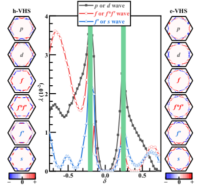
IV.4 Degeneracy between singlet and triplet SCs
The doping-dependences of the largest pairing eigenvalues for all the pairing symmetries are plotted in Fig. 6, where the gap form factors (determined by Eq. (12)) near the two VHS points are shown on both sides. The two green rectangles near the e-VHS and the h-VHS give the regimes for the chiral SO(4) spin-valley DW studied above where , and the remaining regimes support the SC phases. In the regimes near the VHS, the degenerate - and -wave pairings are the leading pairing symmetries, while in the over doped regimes far away from the VHS, the degenerate - and - wave pairings become the leading symmetries.
The most remarkable feature of Fig. 6 lies in that there is a one-to-one corresponding degeneracy between the triplet and singlet pairings, i.e. the - and -pairing degeneracy, the - and -pairing degeneracy, and the - and -pairing degeneracy, see Fig. 7. Similar to the degeneracy between the inter-valley SDW and the VDW, the degeneracy between the inter-valley singlet and triplet pairings originates from that they are related by the unitary symmetry operation defined in Eq. (13). Concretely, the following singlet and triplet pairings with order parameters
| (25a) | ||||
| (25b) | ||||
are related as
| (26) |
where and the operator is defined by Eq. (13). Note that in the weak-pairing limit only the electrons on the FS participate in the pairing, and an electron state on the -th band with momentum can only pair with its TR-partner, i.e. the state on the -th band with momentum . The condition defines as an implicit function of , and from Fig. 7 we have , suggesting that is an odd function of . Equations (25) and (26) suggest that a singlet pairing with even-parity gap function can be mapped to a triplet pairing with odd-parity gap function . In Fig. 7, the distributions of the gap signs for all possible pairing symmetries are schematically shown, where the listed one-to-one mapping between different singlet and triplet pairings can well explain the singlet-triplet degeneracy shown in Fig. 6.
Similar to the degeneracy between the SDW and VDW orders, the degeneracy between the singlet and triplet SCs also originates from the SU(2)SU(2) symmetries. However, there is an important difference between them: for the SC, there is only one “nesting vector” or “wave vector”, i.e., in the particle-particle channel, which is the center-of-mass momentum of a Cooper pair. As a result, the singlet-triplet degeneracy for SC is always tenable, leading to degenerate ground-state energies for singlet and triplet SCs and hence their arbitrary mixing. Such a degeneracy can only be lifted up by adding a weak inter-valley Hund’s-rule coupling that will be studied in the next section.


The doping-dependence of the superconducting shown in Fig. 6 exhibits two asymmetric behaviors consistent with experiments. One is the asymmetry with respect to the CNP: the at the negative dopings is much higher than that at the positive dopings, which is due to the higher DOS for the former case than that for the latter case (see Fig. 2(b)). Such an asymmetric behavior is well consistent with both the experiments of Y. Cao, et al, in Ref. Cao et al. 2018a and the observations of M. Yankowitz, et al, in Ref. Yankowitz et al. 2019. The other asymmetry is with respect to each VH doping: the on the higher-doping side of each VH point is higher than that on its lower-doping side. This asymmetry is attributed to the asymmetric situations of the FS-nesting on the two sides of each VH doping, see Fig. 8 which indicates that the FSs are better nested at the higher-doping side of each VH doping than those at its lower-doping side. As a result, the susceptibility and hence the effective pairing interaction on the higher-doping side of each VH doping are stronger than those on the other side, leading to the higher on the higher-doping side. This asymmetric behavior is also well consistent with both experiments in Refs. Cao et al. 2018a and Yankowitz et al. 2019. The consistence of these two asymmetric doping-dependent behaviors of the with the experiments suggests that the SC pairing mechanism in the MA-TBG should be consistent with that we proposed, i.e. exchanging the spin-valley DW fluctuations.
V Results with weak inter-valley exchange interactions ()
For the realistic material of the MA-TBG, theoretical analysis suggests that there exists a very weak inter-valley Hund’s -rule exchange interaction with strength You and Vishwanath 2019; Isobe et al. 2018; Lee et al. 2019 which has been neglected in Sec. IV. As in the case of , the SU(2)SU(2) symmetry brings about the SDW-VDW degeneracy at the critical point and the singlet-triplet degeneracy for SCs, it’sit is necessary to add the tiny symmetry-breaking -term to lift up these degeneracies. Further more, this symmetry also leads to the chiral SO(4) spin-valley DW ground state which hosts three vectorial DW order parameters, whose polarization directions need to be pinned down by the tiny symmetry-breaking term. In this section, we focus on the infinitesimal term, including and , and investigate its influence on the ground state of the MA-TBG. The two cases will be studied separately in the following.
V.1
For the case of , we set and redo the RPA calculations. The results of our RPA calculations are shown in Figs. 9(a) to 9(d). The doping-dependence of the critical interaction strength shown in Figs. 9(a) suggests , as is verified by the broadened shown in Figs. 9(b). This result suggests that a negative favors the SDW order. In such a case, we redo the energy optimization of the Hamiltonian (3) in the mixed spin-valley DW state determined by Eq. (IV.3), with the same variational parameters. Our result reveals that the pure chiral SDW states Liu et al. 2018 obtained in Sec. IV.2 are the ground states. The physical picture for the evolution from the chiral SO(4) spin-valley DW in the case of to the chiral SO(3) SDW state in the case of is simple: in the former case, due to the SO(4) symmetry, the four axes for each spin-valley DW vectorial order are equally favored, which leads to the free rotation of that vectorial order in the space; however, in the latter case, the VDW-axis for each DW order parameter is disfavored and the left three SDW-axes form the easy “plane”, within which the SDW vectorial orders can arbitrarily rotate.

The chiral SDW state obtained here has similar properties in many aspects with the same phase obtained previously in other contexts Li 2012; Martin and Batista 2008; Kato et al. 2010; Jiang et al. 2014; Liu et al. 2018. The real-space configuration of the chiral SDW state also has four sublattices. This ground state hosts four branches of gapless Goldstone modes, including three spin-wave modes brought about by the spin-SU(2) symmetry breaking and one extra valley-wave modes caused by the valley-U(1) symmetry breaking. At finite temperature, the gapless Goldstone-mode fluctuations will also destroy the long-range DW order, leaving short-ranged DW fluctuations with long correlation length below some characteristic temperature. Further more, the TRS breaking of this state can survive finite temperature. The topological properties of this state can also be nontrivial with nonzero Chern number, as long as an SDW gap opens at the Fermi level.
However, the close proximity of the chiral SDW state obtained here for to the chiral SO(4) spin-valley DW state for makes it different from those in other contexts Li 2012; Martin and Batista 2008; Kato et al. 2010; Jiang et al. 2014; Liu et al. 2018 in the aspect of the response to a weak magnetic field. The condition and the applied weak magnetic field studied in the Sec. IV.3 both have the effect of pinning down the directions of the polarizations of the DW orders. However, the effects brought about by them conflict: while the former case disfavors the VDW, the latter favors it. Considering that the in real materials is very weak, a weak magnetic field (a few Tesla) is enough to overcome its effects. As a result, the weak applied magnetic field would drive the isotropic chiral SDW state here into a nematic DW state containing one nematic VDW order and two nematic SDW orders. Such an effect can be easily checked by experiments.
The doping-dependence of the largest pairing eigenvalues for the singlet and triplet pairing symmetries is shown in Fig. 9(c). Clearly the tiny SU(2)SU(2)-symmetry-breaking -term leads to the split between the singlet and triplet pairings. Concretely, near the VHS the triplet -wave pairing wins over the singlet -wave one and becomes the leading pairing symmetry, while far away from the VHS in the over doped regime the singlet -wave pairing beats the triplet - wave pairing and serves as the leading pairing symmetry. In the experiments reported in Refs. Cao et al. 2018a and Yankowitz et al. 2019, the SC is mainly detected near the VHS. Therefore, the experiment-relevant pairing symmetry in the case of should be triplet -wave pairing. As the -wave belongs to the 2D irreducible representation, the degenerate - and -wave pairings would always be mixed into the form to lower the ground-state energy, i.e. the for abbreviation, as verified by our numerical results. This state is topologically nontrivial. As the is very weak, the two asymmetric behaviors of the doping-dependence of the superconducting shown in Fig. 9(c) are similar with the case of shown in Fig. 6, which are consistent with experiments.
V.2
The RPA results for are shown in Figs. 9(e)- 9(h). Figures 9(e) and 9(f) obviously show , suggesting that the VDW is more favored than the SDW here. However, this does not mean that the ground state for general realistic is in the pure VDW phase, due to the following reason. The tiny positive term as a perturbation on the chiral SO(4) DW state, its only role is to set the VDW-axis as an easy axis for the three vectorial DW order parameters to orient in the space. However, among the three mutually perpendicular , at most one lucky is given the opportunity to orient toward the VDW-axis, with the remaining two still residing in the SDW-“plane”, leading to a mixed VDW and SDW ordered state. Such an argument is consistent with the following numerical results for the succeeding MF-energy minimization. Firstly, the three relative phase angles between the VDW and SDW orders are , keeping the approximate SO(4) symmetry. Secondly, among the three DW order parameters , an arbitrarily chosen one, say , takes the form of , while the remaining two i.e. and , both take the form of with . This result suggests that for , we obtain a spin-valley DW ordered ground state with one scalar VDW order parameter accompanied by another two mutually perpendicular vectorial SDW order parameters, with the three DW order parameters randomly distributed with the three symmetry-related wave vectors .
In Fig. 10, the real-space distributions of the inter-valley charge and spin densities defined in Eq. (23) are shown for a typically chosen group of DW order parameters for this phase, i.e. , , and . As the VDW order in this DW state nearly only takes one wave vector among the three symmetry-related ones , the inter-valley charge density shown in Fig. 10(a) exhibits a nematic stripy structure, which spontaneously breaks the rotational symmetry of the original lattice. Note that the extension direction of the charge stripe can be arbitrary among the three symmetry-related directions. Such a nematic stripy distribution of the inter-valley charge density is related to the recent STM experiments Jiang et al. 2019; Kerelsky et al. 2019. Note that the -symmetry breaking here for the inter-valley charge density can be delivered to the intra-valley one relevant to the STM based on the Ginsberg-Landau theory, as it cannot be excluded that the two orders are coupled. Here we have provided a simple understanding toward these experimental observations based on the spontaneous breaking of the symmetry, which suggests that the is more realistic for the MA-TBG. It’s interesting that the ground state of the system is not a pure nematic VDW, but it also comprises of two additional nematic SDW orders with equal amplitudes, as shown in Fig. 10(b-d) for the three components of the inter-valley spin density. Here we propose that a spin-dependent STM can detect such a nematic spin order, which coexists with the already-detected nematic stripy charge order.
This spin-valley DW ground state hosts four branches of gapless Goldstone modes, including three spin-wave modes brought about by the spin-SU(2) symmetry breaking and one extra valley-wave modes caused by the valley-U(1) symmetry breaking. At finite temperature, the DW fluctuations will also destroy the long-range DW order, leaving short-ranged DW fluctuations with long correlation length below some characteristic temperature. However, the VDW order parameter, the TRS breaking, and the -symmetry breaking can survive the finite temperature, as they are discrete symmetry breakings. Besides, the topological properties of this state can also be nontrivial if it’sit is insulating. Therefore, at finite temperature for , we obtain a nematic VDW state with TRS breaking, which simultaneously hosts strong SDW fluctuations with long spin-spin correlation length.
The doping-dependence of the largest pairing eigenvalues for the singlet and triplet pairing symmetries are shown in Fig. 9(g) for . Consequently, near the VHS the singlet -wave pairing wins over the triplet -wave pairing and becomes the leading pairing symmetry, while far away from the VHS in the over doped regime the triplet -wave pairing beats the singlet -wave pairing and serves as the leading pairing symmetry. The experiment-relevant pairing symmetry near the VH dopings in this case should be singlet -wave pairing, which takes the form of topological pairing state. As the is very weak, the two asymmetric behaviors of the doping-dependence of the superconducting shown in Fig. 9(g) are also clear, which are consistent with experiments.
VI Conclusion and Discussion
In conclusion, by adopting realistic band structure and interactions, we have performed a thorough investigation on the electron instabilities of the MA-TBG driven by FS-nesting near the VH dopings. A particular attention is paid to the approximate SU(2)SU(2) symmetry and the three-folded wave-vector degeneracy brought about by the -rotational symmetry of the system. At the SU(2)SU(2)-symmetric point with , we obtain the chiral SO(4) spin-valley DW state. This state is a generalization of the 3Q chiral SDW state to the VDW-SDW order-parameter space, which is a novel state possessing a series of exotic properties. The leading pairing symmetries are degenerate singlet and triplet . For , we obtain the pure 3Q chiral SDW state, and triplet -wave pairing. For , we obtain a nematic DW state with mixed SDW and stripy VDW orders, and singlet -wave pairing. The stripy inter-valley charge-density pattern in this nematic state is consistent with recent STM experiments, suggesting that is more realistic for the MA-TBG. These results are summarized in Fig. 1. Besides, the two asymmetric doping-dependent behaviors of the pairing phase diagram shown in Fig. 6 and 9 are well consistent with experiments, suggesting the relevance of the exchanging-DW-fluctuations pairing mechanism for the MA-TBG.
The -orbital TB model on the honeycomb lattice adopted here is criticized to be topologically problematic Zou et al. 2018; Po et al. 2019 for the CNP. However, here we focus on the doped case, particularly on the VHS, and therefore only the low-energy band structure near the FS will matter. For more accurate band structure, we can adopt the continuum-theory band structure directly Wu et al. 2018b, which is not only complicated but also has the difficulty of how to properly put in the interaction terms. Alternatively, later than the present work, part of the present authors have recently adopt the faithful TB model Po et al. 2019 with five bands per valley per spin which can properly deal with the band topology to study the problem. Although the band structure of that model is much more complicated than that of our present model, the results published in Ref. Zhang et al. 2020c are qualitatively consistent with those obtained in this work. The reason lies in that the physics discussed in this paper only relies on the approximate SU(2)SU(2) symmetry, the valley-U(1) symmetry and the presence of three-fold degenerate nesting vectors which originate from the -rotational symmetry of the material. These symmetries do not depend on the details of the band structures.
Note that the nesting vectors in our model only locate along the lines, but not exactly at the points. If we adopt the accurate value of (generally incommensurate) to build our VDW or SDW order parameters, the unit cell would be huge or even infinite, which brings great difficulty to the calculations. Further more, the relation might bring further difficulty to the calculations. However, as the main physics revealed here only relies on the three-folded wave-vector degeneracy brought about by the symmetry of the system, we argue that the accurate values of should not influence the main results.
The chiral character of the SO(4) DW state predicted in this work is lack of experiment evidence presently. The reason for this might lie as follow. This state is formed as a consequence of the competition among the three degenerate wave vectors caused by the three-fold rotation symmetry of the system. In realistic system, there might be such factors as the strain which will break the exact three-fold rotation symmetry. As a result, only one of the three wave vectors might win and be realized, which breaks the chiral DW state. Therefore, the state obtained in our work needs ideal experimental condition to be realized, which might be realized in the future. It’s also possible that the weak-coupling start point, as well as the concrete formula of the multi-orbital Hubbard interactions adopted here does not apply to the real material of the magic-angle twisted bilayer graphene system. However, the physics revealed here might apply to other systems with similar degrees of freedom.
Acknowledgements
We are grateful to the stimulating discussions with Noah Fan-Qi Yuan, Yi-Zhuang You, Jun-Wei Liu, Xi Dai, and Long Zhang. This work is supported by the National Natural Science Foundation of China under the Grants No.12074031 (F. Y.), No. 12074037 (Y.Z.), No. 11922401 (C.-C.L.), No. 11874292, No. 11729402 and No. 11574238(Y.W.), No. 11861161001 and No. 12141402 (W.-Q.C.).Z.-C.G. is supported by funding from Hong Kong¡¯s Research Grants Council (NSFC/RGC Joint Research Scheme No. N-CUHK427/18 and General Research Fund Grant No. 14302021). W.-Q.C. is supported by the Science,Technology and Innovation Commission of Shenzhen Municipality (No. ZDSYS20190902092905285), Guangdong Basic and Applied Basic Research Foundation under Grant No. 2020B1515120100, Shenzhen-Hong Kong Cooperation Zone for Technology and Innovation (Grant No. HZQBKCZYB-2020050), and Center for Computational Science and Engineering at Southern University of Science and Technology.
Appendix A Tight-binding Hamiltonian
This Appendix provides some details for the TB Hamiltonian in Eq. (III.1), including its connection with the Slater-Koster formalism and the U(1)-valley symmetry. In addition, how to transform it from the -orbital representation to the valley representation is shown.
The proposed simplest TB model for the MA-TBG possesses two orbitals of and on each lattice site Yuan and Fu 2018; Po et al. 2018; Kang and Vafek 2018; Liu et al. 2018, holding the form,
| (27) |
where is the annihilation operator of the electron with the -th ( represents or ) orbital and spin on the -th site. is the chemical potential and is the hopping integral between the and orbitals on the th and th sites, respectively.
In the case with symmetry, the hopping integral can be constructed Liu et al. 2018 via the Slater-Koster formalism Slater and Koster 1954 based on the coexisting and bondings Wu and Sarma 2008; Wu 2008; Zhang et al. 2014; Liu et al. 2014; Yang et al. 2015, namely,
| (28) |
with denotes the angle from the direction of to that of . The Slater-Koster parameters of and represent the parts of the hopping integrals caused by and bonds between the th and th sites, respectively.
To reflect the U(1)-valley symmetry, the above Slater-Koster Hamiltonian (27) can be transformed into the valley representation via with representing the and valley. As required by the U(1)-valley symmetry, the inter-valley hopping terms should vanish, which leads to,
| (29a) | ||||
| (29b) | ||||
Since , we get
| (30) |
Substituting Eq. (30) into Eq. (28), we have,
| (31) |
Up to the third neighbor hoppings, the Hamiltonian (27) turns into Yuan and Fu 2018; Koshino et al. 2018,
| (32) |
where and denotes the th neighboring bond with the hopping strength of . This Hamiltonian has the valley-SU(2) symmetry.
For the real material of the MA-TBG, the point-group is instead of . The breaking of down to brings about the Kane-Mele type of valley-orbital coupling, i.e.,
| (33) |
where and describes the th neighboring coupling strength.
Combining and , we arrive at the TB Hamiltonian expressed in the Eq. (III.1) of the main text, which satisfies the U(1)-valley symmetry Yuan and Fu 2018; Koshino et al. 2018.
Appendix B More information on RPA approach
In this appendix, we provide the detailed informations on the RPA approach, including the explicit form of the non-interaction susceptibility , the interaction matrices and , and the effective pairing interaction vertex .
The form of is given by
| (34) |
where is the Fermi-Dirac distribution. and represent the the combined index in Eq. (III.1). and are the energy level and corresponding eigenstate at the wave vector for the -th band, both of which are determined by Eq. (III.1). In the RPA level, the renormalized spin and charge susceptibilities have been given in Eqs. (6a) and (6b), in which
| (35a) | ||||
| (35b) | ||||
Labelling orbitals as , the explicit forms of , , and are given as follow. Firstly, the nonzero elements of are:
| (36a) | ||||
| (36b) | ||||
| (36c) | ||||
Secondly, the nonzero elements of are:
| (37a) | ||||
| (37b) | ||||
| (37c) | ||||
| (37d) | ||||
| (37e) | ||||
Finally, the nonzero elements of read:
| (38a) | ||||
| (38b) | ||||
In the expressions of and , , where are the two unit vectors of the Moiré lattice.
In the RPA level, the Cooper pair with momentum and orbital of could be scattered into by exchanging charge or spin fluctuations, see Fig. 11 which is up to the second order perturbation. These processes induce the following effective interaction,
| (39) |
where and denote the opposite-valley bands of the th and th ones, respectively, and . The effective pairing interaction vertex has the form,
| (40) |
The three processes that have contributions to are presented in Fig. 11 where (a) denotes the bare interaction vertex and (b, c) represent two second order perturbation processes. During them the spin or charge fluctuations are exchanged within a cooper pair. The effective vertex is,
| (41) |
for the singlet channel and is,
| (42) |
for the triplet channel.
Note that the vertex has been symmetrized and anti-symmetrized for the singlet and triplet cases, respectively. The vertex gives the effective paring interaction vertex .
Appendix C The G-L theory for the chiral SO(4) DW
C.1 Mixing between VDW and SDW and SO(4) DW
In the main text we prove the degeneracy between the VDW and the SDW. Due to this degeneracy, the two DW order parameters will generally be mixed to lower the energy. Below we study how they would be mixed. The MF Hamiltonian involving both orders should be
| (43) |
where is the mixing angle. We shall show below via combined Ginzburg-Landau (G-L) theory and the microscopic calculations that the mixing angle , under which the SU(2)SU(2) symmetry would be embodied as the SO(4) symmetry for the DW order parameters.
Firstly, due to the global spin-SU(2) symmetry, we can only consider the case in which the spin polarization direction is along the -axis, under which we have
| (44) |
Secondly, the global valley U(1) symmetry of the system requires that when the MF Hamiltonian on the above is operated by the valley U(1) transformation,
| (45) |
the G-L free energy would be unchanged. Under this transformation, we get effectively that
| (46) |
Note that we can combine the phase factor into the definition of and to change the two DW order parameters as complex numbers. Therefore, the G-L free energy of the system can be defined as
| (47) |
The valley U(1) symmetry guarantees that this G-L free energy should be invariant under , which suggests that should come in pair with , i.e.
| (48) |
Thirdly, under the SU(2)SU(2) symmetry, let’s perform the spin-SU(2) transformation only in the valley K,
| (49) |
and not in the valley K’, we have
The G-L free energy should be invariant under this transformation. From Eq. (48), only such combination as can emerge in , where , and are complex matrix. Then from the invariance of under Eq. (C.1), we have
| (59) |
Note that , we have . Therefore, we have
| (60) |
Fourthly, if we perform the global SU(2) rotation: rotate about the spin-x axis by the angle , under which
the free energy function should be invariant. Therefore, the term in Eq. (60) should only appear in even powers.
From the above analysis, the G-L free energy function should take the following form up to the fourth order of ,
| (66) | |||||
where are real numbers. In the case of , the minimization of requires , which dictates that the phase angle of should be different from that of by . In the case of , they should have the same phase angle or be different by a negative sign. Our microscopic calculations always suggest that the former case is realized for the parameters of realistic material. Therefore our combined G-L theory and microscopic calculations suggest that the MF Hamiltonian for the DW ordered state should take the form of
| (67) |
Below we prove that the SU(2)SU(2) symmetry acted on the operator of the system is equivalent to the SO(4) symmetry in the 4D DW order-parameter space when the DW MF Hamiltonian takes the above form Eq. (C.1). Note that , where
| (68) | ||||
It’s important that is an SU(2) matrix because
| (71) |
Mathematically, it’sit is known that any SU(2) matrix can always be parametrized in the form of the equation (C.1).
On the one hand, let’s perform any on the spin of the operator ( valley) and on that of the operator ( valley), resulting in with
| (72) |
Since SU(2), from Eq. (71) we can obtain:
| (73) |
The Eq. (73) suggests that is also an SU(2) matrix, which can also be parametrized in the form of Eq. (C.1) with only and . This leads to an SO(4) rotation on the 4-component DW order parameter . Therefore, we have proved that any SU(2)SU(2) operation acted on the operators will lead to an SO(4) rotation on the 4-component DW order parameter .
On the other hand, suppose that the 4-component DW order parameter in Eq. (C.1) is operated by an SO(4) rotation with , we can always choose
| (74) |
This means that any SO(4) rotation on the 4-component spin-valley DW order parameter can be realized by the physical SU(2)SU(2) operation acted on the operators.
Combining the above two hands, we arrive at our proof.
C.2 Mixing between degenerate wave vectors
On the above subsection, we studied how the SDW and VDW are mixed in the presence of only one wave vector. As a result, they are found to be mixed as 1:i, leading to the SO(4) spin-valley DW. In this subsection, we shall study how the SO(4) DWs with three degenerate wave vectors are mixed via the G-L theory.
In the presence of three degenerate DW orders, the MF Hamiltonian reads,
| (75) |
where the 4-component vector and with to be the identity matrix.
The G-L free energy as a function of the three 4-component vectors can be expanded up to the quartic order of the Taylor’s series as
| (76) | |||||
where and are quadratic and quartic order terms respectively.
Firstly, due to the SO(4) symmetry of the system, the and can only contain such terms as and . As a result, we have
| (77) | |||||
From the rotation symmetry of the system, we know that
| (78) |
Let’s then investigate the consequence of the unit-cell translation symmetry of the system. Setting the unit vector of the original honeycomb lattice as , and the corresponding unit vector in the reciprocal lattice as , we have , and . Let’s translate the system by the unit vector , under which we have
| (79) |
Then Eq. (C.2) suggests that under the unit vector translation, we effectively have
| (80) |
For the case , we have
| (81) |
Then the translational invariance of in Eq.(77) dictates
| (82) |
Similarly, the translational invariance of dictates
| (83) |
Therefore, up to the quadratic order term of , we have
| (84) |
Through similar analysis on symmetry as the above, we can obtain the following symmetry-allowed form of ,
| (85) | |||||
From combined Eq. (84) and Eq. (85), we have
| (86) | |||||
In the following, we shall solve the configurations of which minimize the free energy function provided by Eq. (86).
Firstly, we study the relative orientations among the three DW order parameters . This problem is simply determined by the sign of in Eq. (86). The answer is as following,
| (87) |
Then, we study the relative amplitudes among . Let their amplitudes be . Eq. (C.2) yields that in both cases of and , we have
| (88) | |||||
where
In the long-ranged DW ordered state, we should have
| (92) |
To solve the minimum of the free-energy function provided by Eq. (88), we deform it as
| (93) | |||||
Clearly, the solution for the minimization of function on the above is determined by the sign of . The result is as following,
| (94) |
Note that on the above Eq. (C.2), in the first case , only one of can be nonzero. Such a state is the nematic state, which only hosts one wave vector. In the second case, the amplitudes of the three DW orders are equal, which can either be the chiral SO(4) DW in which the orientations of the three DW order parameters are perpendicular to one another or be the collinear SO(4) DW state in which the orientations of the three DW order parameters are parallel to one another, which is determined by Eq. (C.2).
Summarizing the above derivations, we get the following possible solutions for the minimization of the free energy function defined in Eq. (86)
| , | ||||
| , |
Therefore, only three possible solutions exist, i.e. the collinear SO(4) spin-valley DW state, the chiral SO(4) spin-valley DW state and the nematic SO(4) spin-valley DW state. In the collinear state, the three DW order parameters . In the chiral state, they satisfy and . In the nematic state, only one of the three exists, and the other two vanish. In realistic system, which state would be the ground state cannot be know only from the G-L theory. Instead, the microscopic calculations are needed.
C.3 The case of pure SDW or VDW
In some case in our study we only consider the pure SDW or VDW order parameters, particularly in the case when we try to compare the energies of a pure SDW state and a pure VDW state.
In the case when we consider the pure SDW state, the SDW-MF Hamiltonian reads,
| (101) |
Here denotes the three-component SDW order parameters, which are abbreviated as below. The G-L free energy should be
| (102) |
Adopting the symmetry-based analysis parallel to that performed on the above subsection, we can obtain
| (103) | |||||
The solution for the minimum of Eq. (103) yields
| , | ||||
| , |
Therefore, there are also three possible SDW solutions, i.e. the collinear-SDW state, the chiral-SDW state and the nematic-SDW state. In realistic system, the microscopic calculations are needed to determine which state should be the ground state.
In the case when we consider the pure VDW state, the VDW-MF Hamiltonian reads,
| (110) |
Here denotes the VDW order parameters, which are abbreviated as below. Adopting similar symmetry-based analysis parallel to the above, we can obtain
| (111) | |||||
The solution for the minimum of Eq. (111) yields
| isotropic-VDW | |||||
| nematic-VDW | (112) |
Therefore, there are two possible VDW solutions, i.e. the isotropic-VDW state and the nematic-VDW state. While the former contains three VDW components with equal amplitudes for the three wave vectors, the latter only contains one for one arbitrarily chosen wave vector. In realistic system, the microscopic calculations are needed to determine which state should be the ground state.
References
- Cao et al. (2018a) Y. Cao, V. Fatemi, A. Demir, S. Fang, S. L. Tomarken, J. Y. Luo, J. D. Sanchez-Yamagishi, K. Watanabe, T. Taniguchi, E. Kaxiras, R. C. Ashoori, and P. Jarillo-Herrero, Nature 556, 80 (2018a).
- Cao et al. (2018b) Y. Cao, V. Fatemi, S. Fang, K. Watanabe, T. Taniguchi, E. Kaxiras, and P. Jarillo-Herrero, Nature 556, 43 (2018b).
- Cao et al. (2019) Y. Cao, D. Rodan-Legrain, O. Rubies-Bigorda, J. M. Park, K. Watanabe, T. Taniguchi, and P. Jarillo-Herrero, arXiv:1903.08596 (2019).
- Choi et al. (2019) Y. Choi, J. Kemmer, Y. Peng, A. Thomson, H. Arora, R. Polski, Y. Zhang, H. Ren, J. Alicea, G. Refael, F. v. Oppen, K. Watanabe, T. Taniguchi, and S. Nadj-Perge, Nat. Phys. 15, 1174 (2019).
- Jiang et al. (2019) Y. Jiang, X. Lai, K. Watanabe, T. Taniguchi, K. Haule, J. Mao, and E. Y. Andrei, Nature 573, 91 (2019).
- Kerelsky et al. (2019) A. Kerelsky, L. J. McGilly, D. M. Kennes, L. Xian, M. Yankowitz, S. Chen, K. Watanabe, T. Taniguchi, J. Hone, C. Dean, A. Rubio, and A. N. Pasupathy, Nature 572, 95 (2019).
- Liu et al. (2019a) X. Liu, Z. Hao, E. Khalaf, J. Y. Lee, K. Watanabe, T. Taniguchi, A. Vishwanath, and P. Kim, arXiv:1903.08130 (2019a).
- Shen et al. (2019) C. Shen, N. Li, S. Wang, Y. Zhao, J. Tang, J. Liu, J. Tian, Y. Chu, K. Watanabe, T. Taniguchi, R. Yang, Z. Y. Meng, D. Shi, and G. Zhang, arXiv:1903.06952 (2019).
- Chen et al. (2019a) G. Chen, L. Jiang, S. Wu, B. Lyu, H. Li, B. L. Chittari, K. Watanabe, T. Taniguchi, Z. Shi, J. Jung, Y. Zhang, and F. Wang, Nat. Phys. 15, 237 (2019a).
- Chen et al. (2019b) G. Chen, A. L. Sharpe, P. Gallagher, I. T. Rosen, E. J. Fox, L. Jiang, B. Lyu, H. Li, K. Watanabe, T. Taniguchi, J. Jung, Z. Shi, D. Goldhaber-Gordon, Y. Zhang, and F. Wang, Nature 572, 215 (2019b).
- Chen et al. (2020) G. Chen, A. L. Sharpe, E. J. Fox, Y.-H. Zhang, S. Wang, L. Jiang, B. Lyu, H. Li, K. Watanabe, T. Taniguchi, Z. Shi, T. Senthil, D. Goldhaber-Gordon, Y. Zhang, and F. Wang, Nature 579, 56 (2020).
- Yankowitz et al. (2019) M. Yankowitz, S. Chen, H. Polshyn, Y. Zhang, K. Watanabe, T. Taniguchi, D. Graf, A. F. Young, and C. R. Dean, Science 363, 1059 (2019).
- Xie et al. (2019) Y. Xie, B. Lian, B. Jäck, X. Liu, C.-L. Chiu, K. Watanabe, T. Taniguchi, B. A. Bernevig, and A. Yazdani, Nature 572, 101 (2019).
- Bistritzer and MacDonald (2011) R. Bistritzer and A. H. MacDonald, Proc. Natl. Acad. Sci. 108, 12233 (2011).
- Dos Santos et al. (2007) J. L. Dos Santos, N. Peres, and A. C. Neto, Phys. Rev. Lett. 99, 256802 (2007).
- Chittari et al. (2019) B. L. Chittari, G. Chen, Y. Zhang, F. Wang, and J. Jung, Phys. Rev. Lett. 122, 016401 (2019).
- Wu et al. (2018a) F. Wu, T. Lovorn, E. Tutuc, and A. H. MacDonald, Phys. Rev. Lett. 121, 026402 (2018a).
- Xian et al. (2019) L. Xian, D. M. Kennes, N. Tancogne-Dejean, M. Altarelli, and A. Rubio, Nano Lett. 19, 4934 (2019).
- Tomarken et al. (2019) S. Tomarken, Y. Cao, A. Demir, K. Watanabe, T. Taniguchi, P. Jarillo-Herrero, and R. Ashoori, Phys. Rev. Lett. 123, 046601 (2019).
- Da Liao et al. (2019) Y. Da Liao, Z. Y. Meng, and X. Y. Xu, Phys. Rev. lett. 123, 157601 (2019).
- Hu et al. (2019) X. Hu, T. Hyart, D. I. Pikulin, and E. Rossi, Phys. Rev. Lett. 123, 237002 (2019).
- Yudhistira et al. (2019) I. Yudhistira, N. Chakraborty, G. Sharma, D. Y. Ho, E. Laksono, O. P. Sushkov, G. Vignale, and S. Adam, Phys. Rev. B 99, 140302 (2019).
- Padhi and Phillips (2019) B. Padhi and P. W. Phillips, Phys. Rev. B 99, 205141 (2019).
- Ramires and Lado (2019) A. Ramires and J. L. Lado, Phys. Rev. B 99, 245118 (2019).
- Schrade and Fu (2019) C. Schrade and L. Fu, Phys. Rev. B 100, 035413 (2019).
- Bi et al. (2019) Z. Bi, N. F. Yuan, and L. Fu, Phys. Rev. B 100, 035448 (2019).
- Lin and Nandkishore (2019) Y.-P. Lin and R. M. Nandkishore, Phys. Rev. B 100, 085136 (2019).
- Klebl and Honerkamp (2019) L. Klebl and C. Honerkamp, Phys. Rev. B 100, 155145 (2019).
- Pizarro et al. (2019a) J. Pizarro, M. Rösner, R. Thomale, R. Valentí, and T. Wehling, Phys. Rev. B 100, 161102 (2019a).
- Goodwin et al. (2019a) Z. A. Goodwin, F. Corsetti, A. A. Mostofi, and J. Lischner, Phys. Rev. B 100, 235424 (2019a).
- Zhu et al. (2019) Z. Zhu, D. Sheng, and L. Fu, Phys. Rev. Lett. 123, 087602 (2019).
- Wu et al. (2019a) X.-C. Wu, C.-M. Jian, and C. Xu, Phys. Rev. B 99, 161405 (2019a).
- Goodwin et al. (2019b) Z. A. Goodwin, F. Corsetti, A. A. Mostofi, and J. Lischner, Phys. Rev. B 100, 121106 (2019b).
- Venderbos and Fernandes (2018) J. W. Venderbos and R. M. Fernandes, Phys. Rev. B 98, 245103 (2018).
- Haule et al. (2019) M. Haule, E. Andrei, and K. Haule, arXiv:1901.09852 (2019).
- Kang and Vafek (2018) J. Kang and O. Vafek, Phys. Rev. X 8, 031088 (2018).
- Kang and Vafek (2019) J. Kang and O. Vafek, Phys. Rev. Lett. 122, 246401 (2019).
- Xu et al. (2018) X. Y. Xu, K. Law, and P. A. Lee, Phys. Rev. B 98, 121406 (2018).
- Padhi et al. (2018) B. Padhi, C. Setty, and P. W. Phillips, Nano Lett. 18, 6175 (2018).
- Pizarro et al. (2019b) J. Pizarro, M. Calderón, and E. Bascones, J. Phys. Commun. 3, 035024 (2019b).
- Thomson et al. (2018) A. Thomson, S. Chatterjee, S. Sachdev, and M. S. Scheurer, Phys. Rev. B 98, 075109 (2018).
- Zhang et al. (2019a) Y.-H. Zhang, D. Mao, Y. Cao, P. Jarillo-Herrero, and T. Senthil, Phys. Rev. B 99, 075127 (2019a).
- Liu et al. (2019b) J. Liu, J. Liu, and X. Dai, Phys. Rev. B 99, 155415 (2019b).
- Xie and MacDonald (2020) M. Xie and A. H. MacDonald, Phys. Rev. Lett. 124, 097601 (2020).
- Wu et al. (2019b) X.-C. Wu, A. Keselman, C.-M. Jian, K. A. Pawlak, and C. Xu, Phys. Rev. B 100, 024421 (2019b).
- Yuan and Fu (2018) N. F. Q. Yuan and L. Fu, Phys. Rev. B 98, 045103 (2018).
- Codecido et al. (2019) E. Codecido, Q. Wang, R. Koester, S. Che, H. Tian, R. Lv, S. Tran, K. Watanabe, T. Taniguchi, F. Zhang, M. Bockrath, and C. Ning Lau, Sci. Adv. 5, EAAW9770 (2019).
- Dodaro et al. (2018) J. F. Dodaro, S. A. Kivelson, Y. Schattner, X.-Q. Sun, and C. Wang, Phys. Rev. B 98, 075154 (2018).
- Liu et al. (2018) C.-C. Liu, L.-D. Zhang, W.-Q. Chen, and F. Yang, Phys. Rev. Lett. 121, 217001 (2018).
- Fidrysiak et al. (2018) M. Fidrysiak, M. Zegrodnik, and J. Spałek, Phys. Rev. B 98, 085436 (2018).
- Guo et al. (2018) H. Guo, X. Zhu, S. Feng, and R. T. Scalettar, Phys. Rev. B 97, 235453 (2018).
- Ochi et al. (2018) M. Ochi, M. Koshino, and K. Kuroki, Phys. Rev. B 98, 081102 (2018).
- Lu et al. (2019) X. Lu, P. Stepanov, W. Yang, M. Xie, M. A. Aamir, I. Das, C. Urgell, K. Watanabe, T. Taniguchi, G. Zhang, A. Bachtold, A. H. MacDonald, and D. K. Efetov, Nature 574, 653 (2019).
- Huang et al. (2019) T. Huang, L. Zhang, and T. Ma, Sci. Bull. 64, 310 (2019).
- Rademaker and Mellado (2018) L. Rademaker and P. Mellado, Phys. Rev. B 98, 235158 (2018).
- Classen et al. (2019) L. Classen, C. Honerkamp, and M. M. Scherer, Phys. Rev. B 99, 195120 (2019).
- Kennes et al. (2018) D. M. Kennes, J. Lischner, and C. Karrasch, Phys. Rev. B 98, 241407 (2018).
- Isobe et al. (2018) H. Isobe, N. F. Yuan, and L. Fu, Phys. Rev. X 8, 041041 (2018).
- Sherkunov and Betouras (2018) Y. Sherkunov and J. J. Betouras, Phys. Rev. B 98, 205151 (2018).
- Bultinck et al. (2020) N. Bultinck, E. Khalaf, S. Liu, S. Chatterjee, A. Vishwanath, and M. P. Zaletel, Phys. Rev. X 10, 031034 (2020).
- Kang and Vafek (2020) J. Kang and O. Vafek, Phys. Rev. B 102, 035161 (2020).
- Zhang et al. (2020a) Y. Zhang, K. Jiang, Z. Wang, and F. Zhang, Phys. Rev. B 102, 035136 (2020a).
- Soejima et al. (2020) T. Soejima, D. E. Parker, N. Bultinck, J. Hauschild, and M. P. Zaletel, Phys. Rev. B 102, 205111 (2020).
- Xie et al. (2021) F. Xie, A. Cowsik, Z.-D. Song, B. Lian, B. A. Bernevig, and N. Regnault, Phys. Rev. B 103, 205416 (2021).
- Xu and Balents (2018) C. Xu and L. Balents, Phys. Rev. Lett. 121, 087001 (2018).
- Roy and Juričić (2019) B. Roy and V. Juričić, Phys. Rev. B 99, 121407 (2019).
- Zhang (2019) L. Zhang, Sci. Bull. 64, 495 (2019).
- Ray et al. (2019) S. Ray, J. Jung, and T. Das, Phys. Rev. B 99, 134515 (2019).
- Su and Lin (2018) Y. Su and S.-Z. Lin, Phys. Rev. B 98, 195101 (2018).
- Peltonen et al. (2018) T. J. Peltonen, R. Ojajärvi, and T. T. Heikkilä, Phys. Rev. B 98, 220504 (2018).
- Wu et al. (2018b) F. Wu, A. MacDonald, and I. Martin, Phys. Rev. Lett. 121, 257001 (2018b).
- Lian et al. (2019) B. Lian, Z. Wang, and B. A. Bernevig, Phys. Rev. Lett. 122, 257002 (2019).
- Zhang et al. (2020b) L. Zhang, T. Huang, Y. Liang, and T. Ma, Mode. Phys. Lett. B 34, 2050016 (2020b).
- Brydon et al. (2019) P. Brydon, D. S. Abergel, D. Agterberg, and V. M. Yakovenko, Phys. Rev. X 9, 031025 (2019).
- Angeli et al. (2019) M. Angeli, E. Tosatti, and M. Fabrizio, Phys. Rev. X 9, 041010 (2019).
- Tang et al. (2019) Q.-K. Tang, L. Yang, D. Wang, F.-C. Zhang, and Q.-H. Wang, Phys. Rev. B 99, 094521 (2019).
- Alidoust et al. (2019) M. Alidoust, M. Willatzen, and A.-P. Jauho, Phys. Rev. B 99, 155413 (2019).
- Wu (2019) F. Wu, Phys. Rev. B 99, 195114 (2019).
- Wu and Sarma (2019) F. Wu and S. D. Sarma, Phys. Rev. B 99, 220507 (2019).
- Wang et al. (2019) J. Wang, X. Mu, L. Wang, and M. Sun, Mater. Today Phys. , 100099 (2019).
- Chen et al. (2018) L. Chen, H.-Z. Li, and R.-S. Han, J. Phys.: Cond. Matter. 31, 065601 (2018).
- Liu et al. (2019c) Z. Liu, Y. Li, and Y.-f. Yang, Chinese Phys. B 28, 077103 (2019c).
- Choi and Choi (2018) Y. W. Choi and H. J. Choi, Phys. Rev. B 98, 241412 (2018).
- You and Vishwanath (2019) Y.-Z. You and A. Vishwanath, NPJ Quan. Mater. 4, 1 (2019).
- Gonzalez and Stauber (2019) J. Gonzalez and T. Stauber, Phys. Rev. Lett. 122, 026801 (2019).
- Laksono et al. (2018) E. Laksono, J. N. Leaw, A. Reaves, M. Singh, X. Wang, S. Adam, and X. Gu, Solid State Commun. 282, 38 (2018).
- Wu et al. (2019c) F. Wu, E. Hwang, and S. D. Sarma, Phys. Rev. B 99, 165112 (2019c).
- Fang et al. (2019) S.-C. Fang, G.-K. Liu, H.-Q. Lin, and Z.-B. Huang, Phys. Rev. B 100, 115135 (2019).
- Wu et al. (2019d) X. Wu, W. Hanke, M. Fink, M. Klett, and R. Thomale, arXiv:1909.03514 (2019d).
- Chichinadze et al. (2019) D. V. Chichinadze, L. Classen, and A. V. Chubukov, arXiv:1910.07379 (2019).
- Wu et al. (2021) S. Wu, Z. Zhang, K. Watanabe, T. Taniguchi, and E. Y. Andrei, Nat. Mater. 20, 488 (2021).
- Cea et al. (2019) T. Cea, N. R. Walet, and F. Guinea, Phys. Rev. B 100, 205113 (2019).
- Rademaker et al. (2019) L. Rademaker, D. A. Abanin, and P. Mellado, Phys. Rev. B 100, 205114 (2019).
- Lin and Nandkishore (2018) Y.-P. Lin and R. M. Nandkishore, Phys. Rev. B 98, 214521 (2018).
- Kozii et al. (2019) V. Kozii, H. Isobe, J. W. Venderbos, and L. Fu, Phys. Rev. B 99, 144507 (2019).
- Yuan et al. (2019) N. F. Yuan, H. Isobe, and L. Fu, Nat. Commun. 10, 1 (2019).
- Harshman and Fiory (2020) D. R. Harshman and A. T. Fiory, J. Supercond. Nov. Magn. 33, 367 (2020).
- Po et al. (2018) H. C. Po, L. Zou, A. Vishwanath, and T. Senthil, Phys. Rev. X 8, 031089 (2018).
- Koshino et al. (2018) M. Koshino, N. F. Yuan, T. Koretsune, M. Ochi, K. Kuroki, and L. Fu, Phys. Rev. X 8, 031087 (2018).
- Po et al. (2019) H. C. Po, L. Zou, T. Senthil, and A. Vishwanath, Phys. Rev. B 99, 195455 (2019).
- Li (2012) T. Li, Europhys. Lett. 97, 37001 (2012).
- Martin and Batista (2008) I. Martin and C. Batista, Phys. Rev. Lett. 101, 156402 (2008).
- Kato et al. (2010) Y. Kato, I. Martin, and C. Batista, Phys. Rev. Lett. 105, 266405 (2010).
- Jiang et al. (2014) S. Jiang, A. Mesaros, and Y. Ran, Phys. Rev. X 4, 031048 (2014).
- Nam and Koshino (2017) N. N. Nam and M. Koshino, Phys. Rev. B 96, 075311 (2017).
- Moon and Koshino (2012) P. Moon and M. Koshino, Phys. Rev. B 85, 195458 (2012).
- Fang and Kaxiras (2016) S. Fang and E. Kaxiras, Phys. Rev. B 93, 235153 (2016).
- Dos Santos et al. (2012) J. L. Dos Santos, N. Peres, and A. C. Neto, Phys. Rev. B 86, 155449 (2012).
- Shallcross et al. (2008) S. Shallcross, S. Sharma, and O. A. Pankratov, Phys. Rev. Lett. 101, 056803 (2008).
- Bistritzer and MacDonald (2010) R. Bistritzer and A. H. MacDonald, Phys. Rev. B 81, 245412 (2010).
- Uchida et al. (2014) K. Uchida, S. Furuya, J.-I. Iwata, and A. Oshiyama, Phys. Rev. B 90, 155451 (2014).
- Mele (2011) E. J. Mele, Phys. Rev. B 84, 235439 (2011).
- Mele (2010) E. J. Mele, Phys. Rev. B 81, 161405 (2010).
- Sboychakov et al. (2015) A. Sboychakov, A. Rakhmanov, A. Rozhkov, and F. Nori, Phys. Rev. B 92, 075402 (2015).
- Morell et al. (2010) E. S. Morell, J. Correa, P. Vargas, M. Pacheco, and Z. Barticevic, Phys. Rev. B 82, 121407 (2010).
- Trambly de Laissardière et al. (2010) G. Trambly de Laissardière, D. Mayou, and L. Magaud, Nano Lett. 10, 804 (2010).
- Latil et al. (2007) S. Latil, V. Meunier, and L. Henrard, Phys. Rev. B 76, 201402 (2007).
- De Laissardière et al. (2012) G. T. De Laissardière, D. Mayou, and L. Magaud, Phys. Rev. B 86, 125413 (2012).
- Huang et al. (2018) S. Huang, K. Kim, D. K. Efimkin, T. Lovorn, T. Taniguchi, K. Watanabe, A. H. MacDonald, E. Tutuc, and B. J. LeRoy, Phys. Rev. Lett. 121, 037702 (2018).
- Guinea and Walet (2019) F. Guinea and N. R. Walet, Phys. Rev. B 99, 205134 (2019).
- Gonzalez (2013) J. Gonzalez, Phys. Rev. B 88, 125434 (2013).
- Gonzalez-Arraga et al. (2017) L. A. Gonzalez-Arraga, J. Lado, F. Guinea, and P. San-Jose, Phys. Rev. Lett. 119, 107201 (2017).
- Cao et al. (2016) Y. Cao, J. Luo, V. Fatemi, S. Fang, J. Sanchez-Yamagishi, K. Watanabe, T. Taniguchi, E. Kaxiras, and P. Jarillo-Herrero, Phys. Rev. Lett. 117, 116804 (2016).
- Ohta et al. (2012) T. Ohta, J. T. Robinson, P. J. Feibelman, A. Bostwick, E. Rotenberg, and T. E. Beechem, Phys. Rev. Lett. 109, 186807 (2012).
- Kim et al. (2017) K. Kim, A. DaSilva, S. Huang, B. Fallahazad, S. Larentis, T. Taniguchi, K. Watanabe, B. J. LeRoy, A. H. MacDonald, and E. Tutuc, Proc. Natl. Acad. Sci. 114, 3364 (2017).
- Huder et al. (2018) L. Huder, A. Artaud, T. Le Quang, G. T. de Laissardiere, A. G. Jansen, G. Lapertot, C. Chapelier, and V. T. Renard, Phys. Rev. Lett. 120, 156405 (2018).
- Li et al. (2017) S.-Y. Li, K.-Q. Liu, L.-J. Yin, W.-X. Wang, W. Yan, X.-Q. Yang, J.-K. Yang, H. Liu, H. Jiang, and L. He, Phys. Rev. B 96, 155416 (2017).
- Song et al. (2019) Z. Song, Z. Wang, W. Shi, G. Li, C. Fang, and B. A. Bernevig, Phys. Rev. Lett. 123, 036401 (2019).
- Hejazi et al. (2019) K. Hejazi, C. Liu, H. Shapourian, X. Chen, and L. Balents, Phys. Rev. B 99, 035111 (2019).
- Pal (2018) H. K. Pal, arXiv:1805.08803 (2018).
- Guinea and Walet (2018) F. Guinea and N. R. Walet, Proc. Natl. Acad. Sci. 115, 13174 (2018).
- Zou et al. (2018) L. Zou, H. C. Po, A. Vishwanath, and T. Senthil, Phys. Rev. B 98, 085435 (2018).
- Tarnopolsky et al. (2019) G. Tarnopolsky, A. J. Kruchkov, and A. Vishwanath, Phys. Rev. Lett. 122, 106405 (2019).
- Ahn et al. (2019) J. Ahn, S. Park, and B.-J. Yang, Phys. Rev. X 9, 021013 (2019).
- Chebrolu et al. (2019) N. R. Chebrolu, B. L. Chittari, and J. Jung, Phys. Rev. B 99, 235417 (2019).
- Wu and Sarma (2008) C. Wu and S. D. Sarma, Phys. Rev. B 77, 235107 (2008).
- Wu (2008) C. Wu, Phys. Rev. Lett. 101, 186807 (2008).
- Zhang et al. (2014) G.-F. Zhang, Y. Li, and C. Wu, Phys. Rev. B 90, 075114 (2014).
- Liu et al. (2014) C.-C. Liu, S. Guan, Z. Song, S. A. Yang, J. Yang, and Y. Yao, Phys. Rev. B 90, 085431 (2014).
- Yang et al. (2015) F. Yang, C.-C. Liu, Y.-Z. Zhang, Y. Yao, and D.-H. Lee, Phys. Rev. B 91, 134514 (2015).
- (141) See the Supplementary Materials at…… for the DOS and the FSs at the e-VH and h-VH dopings for five different twist angles near the magic angle, i.e. 1∘, 1.05∘, 1.1∘, 1.15∘, and 1.2∘ .
- Lee et al. (2019) J. Y. Lee, E. Khalaf, S. Liu, X. Liu, Z. Hao, P. Kim, and A. Vishwanath, Nat. Commun. 10, 1 (2019).
- Takimoto et al. (2004) T. Takimoto, T. Hotta, and K. Ueda, Phys. Rev. B 69, 104504 (2004).
- Yada and Kontani (2005) K. Yada and H. Kontani, J. Phys. Soc. Japan 74, 2161 (2005).
- Kubo (2007) K. Kubo, Phys. Rev. B 75, 224509 (2007).
- Kuroki et al. (2008) K. Kuroki, S. Onari, R. Arita, H. Usui, Y. Tanaka, H. Kontani, and H. Aoki, Phys. Rev. Lett. 101, 087004 (2008).
- Graser et al. (2009) S. Graser, T. Maier, P. Hirschfeld, and D. Scalapino, New J. Phys. 11, 025016 (2009).
- Maier et al. (2011) T. Maier, S. Graser, P. Hirschfeld, and D. Scalapino, Phys. Rev. B 83, 100515 (2011).
- Liu et al. (2013) F. Liu, C.-C. Liu, K. Wu, F. Yang, and Y. Yao, Phys. Rev. Lett. 111, 066804 (2013).
- Wu et al. (2014) X. Wu, J. Yuan, Y. Liang, H. Fan, and J. Hu, Europhys. Lett. 108, 27006 (2014).
- Ma et al. (2014) T. Ma, F. Yang, H. Yao, and H.-Q. Lin, Phys. Rev. B 90, 245114 (2014).
- Zhang et al. (2015) L.-D. Zhang, F. Yang, and Y. Yao, Sci. Rep. 5, 8203 (2015).
- Liu and Dai (2019) J. Liu and X. Dai, arXiv:1907.08932 (2019).
- Liu et al. (2019d) J. Liu, Z. Ma, J. Gao, and X. Dai, Phys. Rev. X 9, 031021 (2019d).
- Zhang et al. (2019b) Y.-H. Zhang, D. Mao, and T. Senthil, Phys. Rev. Res. 1, 033126 (2019b).
- Zhang et al. (2020c) M. Zhang, Y. Zhang, C. Lu, W.-Q. Chen, and F. Yang, Chinese Physics B 29, 127102 (2020c).
- Slater and Koster (1954) J. C. Slater and G. F. Koster, Phys. Rev. 94, 1498 (1954).