Snowball sampling from graphs
Abstract
We develop unbiased strategies to probabilistic -wave snowball sampling from graphs, where the interest of estimation may concern finite-order subgraphs such as triangles, cycles or stars. Our approaches encompass also the finite-population sampling strategies to multiplicity sampling and adaptive cluster sampling, both of which can be recast as snowball sampling aimed at graph node totals. A general snowball sampling theory offers greater flexibility in terms of scope and efficiency of graph sampling, in addition to the existing random node or edge sampling methods.
Keywords: Adaptive cluster sampling, incident observation procedure, multiplicity sampling, sample graph, snowball sampling
1 Introduction
By snowball sampling (SBS) starting from an initial sample of units, one would include any additional units that are outside the current sample but can be reached from them at each wave according to a specified observation procedure, and the process is either terminated after a prefixed number of waves (denoted by ) or if no new units can be added. Thus, the sample is observed in the same way as by breadth-first search in a graph, denoted by , where the nodes represent all the units that can be observed by SBS following all possible initial samples, and the edges represent the links among the units to which the observation procedure is applied at each wave.
SBS is not a probability sampling method, if the initial sample of nodes do not have known sampling probabilities, such as when they are obtained merely by convenience, or if the transition from one wave to the next does not strictly follow the specified observation procedure, such as when it relies on the cooperation of survey respondents who do not implement it faithfully. It may still be possible to estimate the parameter on interest by an assumed model of the sampling process, such as the case with respondent driven sampling (Salganik & Heckathorn 2004; Gile et al. 2015, e.g.).
We consider probabilistic SBS from graphs, where the initial node sample is selected with known probabilities and the subsequent observation procedure strictly follows its specification. Goodman 1961 studies a special case of SBS from this perspective, where the out-degree (best friend) is one for every node in a directed graph, and the number of reciprocal edges (mutual best friends) is to be estimated. Frank 1977b; Frank 1979 and Frank & Snijders 1994 consider one-wave SBS from simple graphs to estimate totals over all the nodes. Rebecq 2018 considers one-wave SBS and adaptive cluster sampling (Thompson 1990) following initial Bernoulli sampling to estimate the total number of nodes with specific characteristics in a large network such as Twitter.
Notice that Frank 1971; Frank 1977a; Frank 1978a; Frank 1978b; Frank 1980; Frank 1981 considers estimation for specific subgraphs (such as 2-star or triangle) by graph sampling based on the induced observation procedure, where an edge is observed only if both its end nodes are included in the initial sample, and the probability of observing the subgraphs derives directly from the initial sampling design since no additional sample nodes can be added to the initial sample by induced observation. In contrast, the observation procedure of SBS from graphs is incident, where an edge may be observed from one of its end nodes in the current sample. While this makes it possible to include additional sample nodes wave-by-wave, it also complicates the calculation of the associated sampling probabilities, because a subgraph can be observed in many ways and not all of them need to be realised on a given sampling occasion. Indeed, Zhang & Patone 2017 derive the probability of observing any given subgraph under -wave SBS, , without explaining how the probability can be obtained when the whole graph is only partially observed.
Thus, a general theory for -wave SBS from graphs is needed, where the estimation may concern finite-order subgraphs not limited to the nodes. For example, consider the node set in an undirected simple graph illustrated in Figure 1. The specific characteristics of the subgraph induced by will be referred to as motif, which is triangle in this case, and the order of a motif is simply that of , which is . A motif is said to be induced (Zhang 2021) if it can be determined from the corresponding subgraph alone, regardless how this subgraph may be connected to the rest of the graph. For instance, triangle is an induced motif, but component is not.
In this paper we consider induced motifs of connected subgraphs in simple graphs as the entities of estimation. Some examples of such low-order induced motifs are given in Figure 2. Let contain all the occurrences of some particular motifs in a given population graph , which are of interest, such as all the triangles in . For each , defined for the corresponding subgraph induced by the nodes , let be a fixed value associated with . The corresponding graph total over is given by
| (1) |
In Section 2 we shall develop design-based unbiased strategies to the estimation of under SBS from graphs, where a strategy consists of a method of sampling and an associated estimator, denoted by , and a strategy is unbiased if
where the expectation is taken over hypothetically repeated SBS from the given .
As will be explained in Section 3, our approaches encompass also the existing finite-population sampling strategies to multiplicity sampling (Birnbaum & Sirken 1965; Sirken 1970; Sirken 2005; Lavallée 2007, e.g.) and adaptive cluster sampling (Thompson 1990; Thompson 1991). This is because both these sampling methods can be recast as SBS, where all the units that can be reached at a given wave (according to the specified observation procedure) are included in the sample, although the parameter of interest for these finite-population problems has traditionally been limited to the order-1 motif, i.e. node.
2 Theory
Given a (population) graph , let an initial node sample be selected from according to a known sampling design. Let consist of the nodes that can be observed from next. Specifically, for simplicity of exposition, we assume reciprocal incident observation procedure (RIOP) throughout this section, whereby any node adjacent to a node in is observed, as well as the edge(s) between and , whether the graph is directed or undirected. For , let the -th wave node sample be
The -wave SBS (SBS) is terminated once is obtained; if for some , simply let for . The seed sample of SBS, defined as the nodes to which the specified OP has been applied (Zhang 2021), is given by
| (2) |
The sample graph by SBS is the observed subgraph of , which is given by
where refers to the observed part of the adjacency matrix of according to the RIOP, and contains the nodes that are incident to .
Denote by the observed elements of in . Any node is called a (SBS) ancestor of , , if the selection of in alone would imply the observation of in , i.e.
Denote by all the ancestors of in . Let be a chosen, fixed subset of ancestors, where . Let the corresponding sampling probability
| (3) |
be the probability that at least one node in is selected initially. The estimator
| (4) |
is unbiased for under SBS, where is the 1/0-indicator function. Moreover, let
be the joint sampling probability of . The SBS variance of is given by
Note that (3) and (4) can be calculated only if, for any , one is able to determine given any possible sample graph where is observed, provided which any choice of would yield an unbiased strategy for accordingly. Below we first outline three possible strategies to the choice of , illustrated for the triangle with nodes in Figure 1, before moving on to more detailed development.
I
Let for any , consisting of all its SBS ancestors.
Note that one cannot always observe entirely in a given . For instance, under 3SBS starting from in Figure 1, one would not observe that is also a 3SBS-ancestor of . Thus, additional observations to are generally needed to implement this strategy. Although this is unattractive in many situations, it may still be worth considering, when SBS is carried out to provide a compressed view of a known but very large graph, in order to avoid processing the whole graph.
II
Let be a restricted set of ancestors for any , provided the same can be identified whenever , i.e. whenever is observed in the sample graph starting from any node in .
For instance, under 3SBS given in Figure 1, can always be identified as 3SBS ancestors whenever . Unlike Strategy-I, this one does not require additional observations to .
III
Let for any , where denotes all its SBS ancestors that can be verified in the realised sample graph .
Unlike Strategy-I or II, this one is said to be sample dependent in the sense that another could have been chosen insofar as is unknown in advance. For example, one can let if 3SBS starts from in Figure 1; whereas would not have been possible had 3SBS started from . This strategy does not require additional observation to either, and it is computationally the least demanding of all the strategies outlined here.
2.1 Strategy-I
The induced (motif of) subgraph is observed iff . The observation distance from a node to is the number of waves it takes from to observe , denoted by . A node is a SBS ancestor of if . Below we first explain the calculation of and then provide the result that is needed to use in (3).
Let be the geodesic distance from node to in , which is the number of waves it takes from to observe . For example, in Figure 1, we have , , and . Let if cannot be observed from . Given the RIOP, whether the graph is directed or undirected.
The geodesic distance from a node to a motif in is defined as the number of waves it takes from to observe any of the nodes , and it is given by
| (5) |
For the motif with in Figure 1, we have , , and .
The number of waves it takes from a node to observe all the nodes is called the radius distance from to in , and it is given by
For the motif with in Figure 1, we have , , and .
Lemma 1.
For a node and an induced motif of connected , we have
Lemma 2.
For any induced motif of connected , which is observed by SBS, one needs at most additional waves to observe .
The Lemmas 1 and 2 can be applied for Strategy-I; see Appendix A for the proofs. Notice that there is a possibility of empty ancestor set if is too small, in which case one can increase till for at least some . For example, for any triangle , we have under 1SBS and under 2SBS, because a triangle can only be observed in two waves from any of its nodes . Meanwhile, it is still possible to observe the triangle by 1SBS if at least two nodes in are selected in . Similarly for many other motifs. Thus, more generally for SBS, one can allow sets of nodes as the joint ancestors of a given , and let all its SBS ancestors be given by
where is the observation distance from a node set to a motif . An unbiased estimator can then be given similarly to (4) on replacing for . However, we do not pursue such a generalisation in this paper because we have not yet clarified all the computational aspects.
2.2 Strategy-II
By this strategy one must be able to verify the same restricted ancestor set , whenever is observed in starting from any node in . Below we provide some results by which can be specified regardless the realised . The proofs are given in Appendix A.
Corollary 1.
For any induced motif of connected , a restricted set of SBS ancestors is given by
Corollary 1 follows directly from Lemma 2. It can be quite restrictive. One can often obtain a larger restricted set by the next result, for which it is convenient to introduce
as the diameter of a given motif in , and
as its observation diameter in . By Lemma 1, if , then we have
Lemma 3.
For any induced motif of connected , a restricted set of SBS ancestors is given by
where is as given in Corollary 1, and .
The restricted set given by Corollary 1 is clearly a subset of that by Lemma 3. But there is still room for improving Lemma 3. Take the triangle with in Figure 1. Corollary 1 is not effective under 2SBS, because but for any node . We have for Lemma 3, so that because is empty. The result below can be useful when is even.
Lemma 4.
For any induced motif of connected , where , let be given by Lemma 3 for SBS, where is even. A restricted set of SBS ancestors is given by
By Lemma 4 one can now include in for 2SBS in addition to . Meanwhile, we have under 2SBS in this graph, and all the nodes can be identified as 2SBS ancestors whenever is observed, where can be observed from either or as fast as from any node in . It may therefore still be possible to improve the Lemmas 3 and 4 by future research.
2.3 Strategy-III
Recall that by definition contains all the SBS ancestors, for any given , which can be identified in the realised sample graph . Let be the sample observation distance calculated in (as if it were ), where generally.
Lemma 5.
For any induced motif of connected observed by SBS, we have
The Lemma 5 establishes as a viable strategy; see Appendix A for the proof. Note that for each , there exists at least a path corresponding to in the sample subgraph that is induced by , denoted by , whose edge set is given by instead of . This is because any node on the path giving rise to must have a shorter sample observation distance to than , which means that it must belong to . Thus, to identify , one simply needs to check, for , the sample subgraph induced by the nodes
where by default, to find any node in with , until no such nodes exist at some .
Take in Figure 1 for an illustration. We have for 1SBS, and for 2SBS. For 3SBS, and it is possible to let
Now, for any with , it is possible for to vary with the realised sample graphs . One can envisage a sequence of sample graphs generated by repeated sampling from , by which is fixed for every (in ) according to the first where , i.e. the first time the motif can be used for estimation by Strategy-III. Denote the resulting collection by
There is only a finite number of distinct collections , and each yields a SBS variance of the estimator (4) under the Strategy-III. An illustration will be given in Section 3.1 later. Meanwhile, based on the sample graph , an estimator of requires only for each in . It follows that the variance estimator is aimed at the weighted average of the sampling variances corresponding to all the collections that are compatible with the realised , where the weight of each derives from the probability of its corresponding sequences of sample graphs starting with the realised . Thus, a variance estimator that is unbiased for the conditional variance given is also an unbiased estimator of the unconditional variance of Strategy-III over repeated sampling.
3 SBS for population totals
3.1 Multiplicity sampling
In finite-population multiplicity sampling, each measurement (or study) unit is accessed indirectly via one or several sampling units, such as when patients of a certain disease (measurement units) are sampled via the medical centres (sampling units) at which they receive treatments, or when a group of adult siblings (measurement units) are sampled via their respective households (sampling units) by referring to each. The multiplicity of a measurement unit is then the (number of) sampling units that can lead to it (Birnbaum & Sirken 1965). Traditionally, the knowledge of multiplicity must be collected in the survey, in order to calculate the sampling probability of each observed measurement unit. Below we explain how one can recast finite-population multiplicity sampling as SBS from graphs, whereby unbiased estimation of defined by (1) over all the measurement units becomes achievable even when the full knowledge of multiplicity cannot be obtained by surveying the sampled measurement units.
Let the population graph be a bipartite graph , where denotes of all the sampling units and all the measurement units, and denotes the edges that only exist from to but not between any two nodes in (or ). Let iff the selection of in leads to the observation of in according to the given multiplicity sampling method. For SBS from , let the initial sample be selected from , which leads to the sample of measurement units by the RIOP, . To collect the knowledge of multiplicity via survey is then the same as applying an extra 2nd wave of SBS from , yielding the 1SBS ancestor set for each sampled . In other words, traditional finite-population multiplicity sampling amounts to applying Strategy-I to 1SBS from such a bipartite graph.
Suppose now the extra 2nd wave of SBS is infeasible due to the survey reality, such that the traditional methods (Birnbaum & Sirken 1965; Sirken 1970; Sirken 2005; Lavallée 2007, e.g.) cannot be applied. Neither is Strategy-II feasible here for 1SBS by the Lemmas 3 and 4. To illustrate how the sample-dependent Strategy-III can be applied for 1SBS in such situations, consider the simple bipartite graph in Figure 3 (top), with the sampling units and measurement units . Let . Suppose simple random sampling without replacement (SRS) of , and .
As explained in Section 2.3, let each collection of sample-dependent ancestor sets be generated by a sequence of 1SBS from this graph. For instance, depicted in the middle of Figure 3 can result from on the first occasion and on the second occasion. Notice that first chosen given would remain fixed, although will be observed to be another ancestor of later. In comparison, depicted at the bottom of Figure 3 can result from on the first occasion and on the second occasion.
| Strategy | (if unstated) | Multiplicity | ||
| I | (1,2,3,2,1,1,1) | 0.202 | 2.987 | |
| III, case 1 | , | (1,2,2,1,1,1,1) | 0.322 | 6.333 |
| III, case 2 | , | (1,2,2,1,1,1,1) | 0.165 | 1.000 |
| III, case 3 | (1,2,2,2,1,1,1) | 0.248 | 3.507 | |
| III, case 4 | , | (1,1,1,1,1,1,1) | 0.274 | 3.667 |
| , | ||||
| III, case 5 | , , | (1,1,2,1,1,1,1) | 0.410 | 8.467 |
| , , | ||||
| III, case 6 | (1,2,1,2,1,1,1) | 0.322 | 6.653 | |
| III, case 7 | , | (1,1,1,2,1,1,1) | 0.351 | 6.867 |
| , |
For the population graph at the top of Figure 3, Table 1 summarises the seven possible 1SBS variances of given by (4), referred to as cases 1 to 7, which can result from the sample-dependent Strategy-III, in comparison with the traditional Strategy-I that requires an extra wave of SBS. Note that the two discussed above actually lead to the same sampling variance, which are given as the two variations of case 5 in Table 1. The sample-dependent ancestor set can only vary for a measurement unit with , which are here; the sizes of are given in italics for these three measurement units in Table 1. Finally, the coefficient of variation (CV) of the observed number of measurement units is also given, which is seen to be correlated with here.
| Case 2 | Case 5 | |||
| 6.4 | 7.2 | |||
| 6.4 | 5.2 | |||
| 8.4 | 11.2 | |||
| 6.4 | 2.0 | |||
| 8.4 | 9.2 | |||
| 6.0 | 7.2 | |||
| 7.0 | 7.0 | |||
| 1.000 | 8.467 | |||
The sampling variance of Strategy-III is lowest in case 2, where it is even more efficient that Strategy-I that requires an extra wave of SBS. The collection in this case differs to only in terms of and , where is excluded from and . The sampling variance of Strategy-III is highest in case 5, for which the two collections have been given in Figure 3. Table 2 compares the details for these two cases given all the six possible initial samples , where in the middle of Figure 3 is used for illustrating case 5 here. The association between and and its effect on the sampling variance are quite obvious in this SBS problem. Another indicator for the sampling variance of Strategy-III is the variability in the number of measurement units associated with each sampling unit given the collection , which is
We have in case 2, which has much less variability compared to or in case 5.
3.2 Adaptive Cluster Sampling
Adaptive cluster sampling (ACS) from finite populations starts with an initial sample and adaptively adds units to the current sample if they satisfy a criterion specified in advance. Thompson 1990; Thompson 1991 considers sampling from that consists of a set of spatial grids over a given area, where each grid is associated with an amount of a species of interest, denoted by for . The initial grid sample may be draw directly from or via some primary sampling units as in two-stage ACS. Given any , one would survey all its neighbour grids (in four directions if possible) only if exceeds a threshold value. The observation is repeated for all the neighbour grids, which may or may not generate further grids to be surveyed. The process is terminated, when the last observed grids are all below the threshold. The interest is to estimate the total .
By recasting finite-population ACS as SBS from graphs, we explain below how the proposed strategies for SBS can extend the approach to ACS proposed by Thompson 1990. For illustration we use the “small” example of Thompson 1990, where the population consists of 5 spatial grids with -values and contiguity as represented by the edges in the top graph in Figure 4. Notice that, following Thompson 1990, we simply denote each node (or grid) by its -value.
ACS from the top graph in Figure 4 is the same as SBS from the bottom graph by the forward (rather than reciprocal) incident observation procedure. A node with -value below the threshold may be called a terminal node because it does not lead to any other nodes. A terminal node is called an edge node, if it is adjacent to at least one non-terminal network (NTN), which consists of a cluster of connected non-terminal nodes whose -values all exceed the threshold, such as in Figure 4. All the nodes in an NTN are observed under SBS iff at least one of them is selected in ; observing an NTN would lead one to observe all its edge nodes, but not the other way around.
Thus, all the nodes belonging to the same NTN have this NTN as their SBS ancestors, such as in Figure 4. For any terminal node that is not an edge node, its ancestor set is simply itself, , such as and . The ancestor set of an edge node includes itself and all its adjacent NTNs, such as . Notice that for as the total of over , the motif of interest is node and no distinction between and is necessary here.
For Strategy-I (Section 2.1), notice that one cannot observe of any edge node by additional waves of observation, unless all its adjacent NTNs intersect the initial , because additional waves cannot progress from . Thompson 1990 proposes to modify the estimator (4), whereby an edge node is used in estimation only if it is selected in directly, the probability of which can be calculated, but not when it is observed via its adjacent NTN. Denote this as Strategy-I∗ below due to the modified estimator .
There is a strong connection to Strategy-II (Section 2.2) using the estimator (4), where one can let be the restricted ancestor set of any terminal node , whether or not it is an edge node, which is possible since (or ) is known. One can let for any non-terminal node, which can be observed under SBS whenever is sampled.
As a matter of fact one obtains the same estimate under the Strategy-II or I∗. The difference is that would be unchanged by Rao-Blackwellisation, whereas would; as will be illustrated below.
Finally, the sample-dependent Strategy-III (Section 2.3) can be applied with for any non-edge node . For an edge node, i.e. 2 in this example, the ancestors can e.g. be chosen as follows:
- (a)
if , use ;
- (b)
if , use .
| I∗ | II | III, | ||||
| Sample | Sample | Sample | ||||
| 0,1 | 0,1 | 0.500 | 0,1 | 0.500 | 0,1 | 0.500 |
| 0,2 | 0,2 | 1.000 | 0,2 | 1.000 | 0,2 | 0.444 |
| 0,10 | 0,10,2,1000 | 288.571 | 0,10,1000 | 288.571 | 0,10,2,1000 | 289.016 |
| 0,1000 | 0,1000,2,10 | 288.571 | 0,1000,10 | 288.571 | 0,1000,2,10 | 289.016 |
| 1,2 | 1,2 | 1.500 | 1,2 | 1.500 | 1,2 | 0.944 |
| 1,10 | 1,10,2,1000 | 289.071 | 1,10,1000 | 289.071 | 1,10,2,1000 | 289.516 |
| 1,1000 | 1,1000,2,10 | 289.071 | 1,1000,10 | 289.071 | 1,1000,2,10 | 289.516 |
| 2,10 | 2,10,1000 | 289.571 | 2,10,1000 | 289.571 | 2,10,1000 | 289.016 |
| 2,1000 | 2,1000,10 | 289.571 | 2,1000,10 | 289.571 | 2,1000,10 | 289.016 |
| 10,1000 | 10,1000,2 | 288.571 | 10,1000 | 288.571 | 10,1000,2 | 289.016 |
| Variance | 17418.41 | 17418.41 | 17482.35 | |||
For the numerical details of the various strategies in Table 3, we let the initial sample size be and select from by SRS, where the adaptive threshold is . For the Strategy-I∗, the edge node is given in italic in the five samples where it is observed but unused for estimation. The probability for this is , which is just the sampling probability of the node 2 under Strategy-II. Otherwise, the observed sample of nodes are always the same under both the strategies, as well as the estimate. Nevertheless, the two differ regarding the Rao-Blackwell method. The difference hinges on the last three cases here, where the sample is the same but is unused by Strategy-I∗ when . The Rao-Blackwell estimate in these three cases is . In contrast, the estimate by Strategy-II is unchanged by Rao-Blackwellisation, because the sample used for estimation differs from to that from or .
For the sample-dependent Strategy-III, there exist two different ancestor sets for the edge node 2, depending on how it is actually observed. The results with , given either or , are the same as those from Strategy-II, which are therefore omitted from Table 3. The results with given are presented. The unconditional variance of by Strategy-III is , averaged over the two distinct collections depending on . It is less efficient than Strategy-II here, because the sampling probability of the edge node 2 is lower or equal under Strategy-II, which is more reasonable given that an edge node by definition has a relatively small -value below the threshold. This can be easily amended under Strategy-III by setting to be a proper subset of .
4 SBS for lower-order subgraphs
Instead of node totals as in finite-population sampling, we now consider the totals of the other motifs defined for lower-order subgraphs in Figure 2, i.e. edge (), 2-star (), triangle (), 4-cycle (), 4-clique (), 3-star () and 3-path (). First, in Section 4.1, the Strategies-II and III are illustrated for a simulated population graph and compared to graph sampling by induced observation. Next, in Section 4.2, some other graphs are used to further explore how the relative graph sampling efficiency might vary.
4.1 A population graph with 50 nodes and 79 edges
Figure 5 shows a population graph with nodes and edges, the top central part of which has been given as Figure 1 earlier. The graph totals of interest here are

4.1.1 Some computational details
Before presenting the results of relative efficiency in Section 4.1.2, let us first explain some computational details of the SBS strategies by an example in terms of , and .
Let be the initial sample by SRS from . The resulting sample graphs by SBS for are given in Figure 6. None of the three motifs , and is observed by . Only the nodes are yet unobserved by the 4th wave, where the first three have degree zero (i.e. isolated nodes). All the edges incident to the nodes are observed, but not all of those incident to .
For any observed sample motif by given , let be the multiplicity of its SBS ancestor set, and let or be that by Strategy-II or III. The motif can be used for estimation by Strategy-II if , whereas it can be used by Strategy-III if . Given SRS of the initial , the probability (3) is given by
where , and or depending on the adopted strategy.

| Motif | SBS | Nodes | |||
|---|---|---|---|---|---|
| 4 | 4 | 4 | |||
| 4 | 5 | 5 | |||
| 4 | 5 | 5 | |||
| 4 | 6 | 6 | |||
| – | 5 | 7 | |||
| – | 5 | 5 | |||
| – | 14 | 16 | |||
| – | 14 | 15 | |||
| – | 14 | 15 | |||
| – | 16 | 17 | |||
| – | 16 | 16 | |||
| – | 17 | 17 | |||
| – | 17 | 17 | |||
| 4 | 4 | 4 | |||
| 14 | 15 | 15 | |||
| 14 | 14 | 14 | |||
| 14 | 31 | 31 | |||
| 14 | 27 | 27 | |||
| – | 25 | 28 | |||
| – | 11 | 12 |
Take first the triangle , the number of which is in Figure 5. Table 4 lists the six triangles that are observed by 2SBS from and their multiplicity . The estimate of is 25.8 by Strategy-II and 31.7 by Strategy-III.
- (a)
For Strategy-II, as explained in Section 2.2, Lemma 3 yields for any triangle under 2SBS, whereas Lemma 4 yields additionally any node that is adjacent to all the nodes , such as the node 30 for in Table 4. Hence, we have and for all the first four triangles. No such additional nodes exist for the fifth or sixth triangle, for which we have and , such that neither is used in estimation although both are observed.
- (b)
For the sample-dependent Strategy-III, we only need to identify the 2SBS ancestors in the sample graph in Figure 6 directly, such as for , for , and so on.
Consider next the 4-cycle , for which in Figure 5. Given , no 4-cycle is observed by while seven of them are observed by (Table 4). The estimate does not exist by Strategy-II, while it is 13.4 by Strategy-III.
- (c)
Under 3SBS, only Lemma 3 is applicable for Strategy-II, which yields as the union of and any other node with observation distance . However, no such additional nodes (outside exist for these seven 4-cycles, such that . Since for all the 4-cycles here, none of them can be used by Strategy-II.
- (d)
Finally, there are only four 4-cliques in Figure 5. Given , all of them are observed by (Table 4).
- (e)
Only the motif with is observed by , for which we have , such that and either by Strategy-II or III.
- (f)
One more 4-clique is observed by . For Strategy-II by Lemma 3, is the union of and any node that is adjacent to at least one of . By Strategy-III, one additional node 8 is included in for , which is two steps away from any node in . The probability is if or if , yielding or 4.0 either by Strategy-II or III.
- (g)
The last two 4-cliques observed by are not used by Strategy-II, since for them. Hence, as by the same strategy under 3SBS. In contrast, all the observed motifs are used by Strategy-III, yielding .
4.1.2 Results
Table 5 provide some results of relative efficiency for totals of all the motifs in Figure 5 mentioned at the beginning of Section 4. SBS either by Strategy-II or III is compared to graph sampling by induced observation following initial SRS; the sample size for the latter is set to the expected node sample size by the corresponding SBS.
| Strategy | ||||||||
|---|---|---|---|---|---|---|---|---|
| III | 0.26 | – | – | – | – | – | – | |
| II, Corollary 1 | 0.26 | – | – | – | – | – | – | |
| II, Lemma 3 | 0.26 | – | – | – | – | – | – | |
| III | 1.63 | 0.76 | 0.50 | 0.08 | 0.16 | 1.31 | 0.71 | |
| II, Corollary 1 | 2.18 | – | – | – | – | – | – | |
| II, Lemma 3 | 2.18 | 0.74 | 0.57 | 0.08 | 0.16 | 1.39 | 0.69 | |
| II, Lemma 4 | 2.25 | 0.76 | 0.57 | 0.08 | 0.16 | 1.39 | 0.70 | |
| III | 5.13 | 1.78 | 0.61 | 0.24 | 0.29 | 1.25 | 1.12 | |
| II, Corollary 1 | 5.80 | 3.38 | 2.54 | 0.94 | 1.25 | 8.03 | 3.44 | |
| II, Lemma 3 | 5.80 | 3.38 | 0.93 | 0.26 | 1.25 | 1.42 | 1.73 | |
| III | 5.82 | 2.21 | 0.85 | 0.41 | 0.24 | 1.51 | 1.22 | |
| II, Corollary 1 | 14.42 | 8.79 | 6.98 | 3.45 | 3.91 | 23.23 | 9.14 | |
| II, Lemma 3 | 14.42 | 4.91 | 2.54 | 0.94 | 1.10 | 2.24 | 3.51 | |
| II, Lemma 4 | 13.19 | 4.96 | 2.27 | 0.94 | 1.08 | 2.25 | 3.75 |
For these results we let by SRS for SBS with , where a large part of the graph may already have been observed by as illustrated above in Section 4.1.1. Given the observation diameters of , we need to apply the SBS strategies in Section 2 except for edge . The restricted ancestor set for Strategy-II is given by Corollary 1, Lemma 3 or Lemma 4 (in case is even), where Corollary 1 is only applicable for edge under 2SBS. An observed sample motif is used by Strategy-II if , or by Strategy-III if .
The unconditional variance of Strategy-III cannot be evaluated here due to the large number of possible . In Table 5 we report the conditional variance given the following . Let a hypothetical sequence of be , , , , , , , , , where the nodes 39 to 50 correspond to , , , , , , , , , , and . Going through one by one in this sequence, we let be given according to the first sample graph where for each relevant motif , until we obtain . Although this conditional variance differs to the unconditional variance of Strategy-III, the comparisons to be discussed below are robust against this difference.
Given the observed sample of motifs under graph sampling by induced observation following initial SRS of size (from nodes), the Horvitz-Thompson estimator (Horvitz & Thompson 1952) of defined by (1) is given by
where
for any , and its sampling variance is
where
for and for any .
It can be seen from Table 5 that, for Strategy-II, Lemma 3 can yield great efficiency gains over Corollary 1, but the difference to Lemma 4 is little here. For , the sample-dependent Strategy-III can be much more efficient than Strategy-II, whereas graph sampling by the induced observation procedure is more efficient than SBS by Strategy-III for the star-like motifs but less efficient for the clique-like motifs .
The results for the edge total seems particularly instructive, where SBS is much more efficient than induced graph sampling with but much less efficient as increases. As increases, so does the variability in the multiplicity (or sampling probability ) over , which is not desirable here since over . For example, by Strategy-III, the range of for edges is with , with , with and with . In contrast, the sample inclusion probability is the same for all the edges under induced graph sampling following initial SRS, i.e. 0.0171, 0.1396, 0.4049 or 0.6367 for or 4 here.
Of course, this also suggests that the relative efficiency of SBS could improve if the value of interest (associated with motif ) tends to be higher in the denser parts of the graph (i.e. instead of considered here). For example, the bottom part of the population graph in Figure 5 is more dense than the other parts of the graph. If a node in this part is selected in , we would observe relatively more edges (and other motifs) as increases, compared to induced graph sampling. If such variations of are positively associated with , then the relative efficiency of SBS would improve.
4.2 Some further exploration
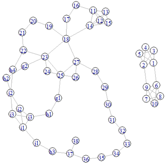
The results in Section 4.1.2 suggest that, given for all , the relative efficiency of SBS may be improved if the nodes in the population graph have a more even degree distribution. Figure 7 shows another population graph with the same number of nodes and edges as that in Figure 5, but apparently with a much more even degree distribution; it mainly consists of cycles and some small cliques (up to order 5).
| SBS | Strategy | |||||||
|---|---|---|---|---|---|---|---|---|
| III | 0.17 | – | – | – | – | – | – | |
| II, Corollary 1 | 0.17 | – | – | – | – | – | – | |
| II, Lemma 3 | 0.17 | – | – | – | – | – | – | |
| III | 0.72 | 0.19 | 0.24 | 0.04 | 0.02 | 0.31 | 0.23 | |
| II, Corollary 1 | 0.62 | – | – | – | – | – | – | |
| II, Lemma 3 | 0.62 | 0.22 | 0.24 | 0.04 | 0.02 | 0.31 | 0.23 | |
| II, Lemma 4 | 0.66 | 0.22 | 0.24 | 0.04 | 0.02 | 0.31 | 0.23 | |
| III | 2.39 | 0.35 | 0.60 | 0.17 | 0.03 | 0.28 | 0.19 | |
| II, Corollary 1 | 1.78 | 0.53 | 0.74 | 0.18 | 0.13 | 1.27 | 0.87 | |
| II, Lemma 3 | 1.78 | 0.53 | 0.63 | 0.17 | 0.13 | 0.34 | 0.31 | |
| III | 4.98 | 0.63 | 1.05 | 0.35 | 0.08 | 0.27 | 0.29 | |
| II, Corollary 1 | 3.72 | 1.15 | 1.59 | 0.51 | 0.42 | 3.00 | 2.05 | |
| II, Lemma 3 | 3.72 | 0.68 | 1.36 | 0.46 | 0.08 | 0.31 | 0.63 | |
| II, Lemma 4 | 4.39 | 0.70 | 1.44 | 0.47 | 0.09 | 0.31 | 0.64 |
Table 6 presents the results of relative efficiency in parallel to Table 5, where the initial sample size for induced graph sampling is now or 27 for or 4. For Strategy-II, we observe the same pattern of relative efficiency among Corollary 1, Lemma 3 and Lemma 4. Next, the differences between Strategy-III and Strategy-II (by Lemma 3 or 4) have reduced considerably compared to those for Figure 5. Finally, except for the edge total, SBS by Strategy-III is mostly more efficient than graph sampling by induced observation including the star-like motifs .
| 50-cycle | (48-clique, 2-clique) | ||||
|---|---|---|---|---|---|
| 0.0012 | 0.0052 | 0.0478 | 0.0873 | 135.23 | 5.72 |
| 1 | 2 | 3 | 4 | 5 | 6 | 7 | 8 | 9 | 10 | |
|---|---|---|---|---|---|---|---|---|---|---|
| 6 | 6 | 21 | 21 | 36 | 36 | 50 | 50 | 63 | 63 | |
| 5156 | 1186 | 445 | 243 | 142 | 85 | 52 | 32 | 19 | 13 | |
| 5 | 9 | 13 | 16 | 19 | 22 | 25 | 28 | 31 | 33 |
Focusing on the edge total, we now construct two more extreme population graphs: (i) a 50-cycle, and (ii) a two-component graph of a 48-clique and a 2-clique. Table 7 presents the relative efficiency of SBS by Strategy-II following SRS of with , against induced graph sampling following initial SRS with comparable sample size . The restricted ancestor set is either given by Lemma 3 if is odd or by Lemma 4 if is even. Notice that for the second population graph (48-clique, 2-clique), we let at most, because the sample graph would not change after two waves no mater how is distributed between the two components of the graph.
Clearly, the relative efficiency of SBS given is considerably improved given a more even degree distribution in the population graph. Indeed, may be the most efficient choice of for edge total estimation in an -cycle graph, because the number of observed sample edges would be a constant as long as the initial sample nodes are at least two steps away from each other. Whereas as increases, the chance would increase for the observed paths (from each initial sample node) to overlap by varying extent, which would result in an increase of the sampling variance for edge total estimation. Table 8 shows the sampling variance by Strategy-II under SBS from the 50-cycle graph, for , as well as that of induced graph sampling following initial SRS of comparable sample sizes. It can be seen that the SBS sampling variance is indeed the lowest at . In comparison, the sampling variance of induced graph sampling decreases in a monotone fashion as increases. The relative efficiency is almost equal to one at in this case, afterwards induced graph sampling becomes more efficient than SBS.
5 Final remarks
Graph sampling (Zhang 2021; Zhang & Patone 2017) provides a statistical approach to study real graphs, whether the graph is only partially observed in terms of the sample graph or if the graph is in principle known but various compressed views of it are desirable (compared to processing the whole graph). In the above we have developed a general theory for SBS from graphs. It encompasses the relevant works on probabilistic SBS from graphs or finite populations, thereby extending the scope of application of snowball sampling. In situations where the estimation objective is also achievable by other methods, such as induced graph sampling, the theory provides one with a greater choice of design-unbiased strategies and the means to improve graph sampling efficiency in practice. Below we shortly point out some topics for future research.
Just like the estimator for ACS proposed by Thompson 1990 can be viewed as a modification of the estimator (4) under Strategy-I for SBS, other estimators are possible under the outlined SBS strategies. Indeed, Patone & Zhang 2022 develop a large class of design-unbiased incidence weighting estimators, which greatly extends the work of Birnbaum & Sirken 1965 and includes the estimator (4) as a special case. This broad class of estimators are applicable to SBS given any of the Strategies I-III to , although an investigation of such extensions of (4) is beyond the scope of the current paper. Other unbiased or nearly unbiased estimators may be discovered in future.
As discussed at the end of Section 2.1, SBS ancestors can be generalised from nodes to sets of nodes. Provided one can handle the required graph computations, this would introduce additional possibilities for improving the efficiency of graph sampling.
The incident observation procedure of SBS considered in this paper is the same as that of breadth-first search in graphs, which includes all the adjacent nodes that can be reached from a current node, possibly subjected to the direction of observation. In contrast, depth-first observation would include only one of these adjacent nodes, as in various random-walk related sampling methods (Thompson 2006b; Zhang 2021; Zhang 2022, e.g.). Hybrid procedures of breadth- and depth-first observation can be envisaged, such as adaptive web sampling (Thompson 2006a). Further development of hybrid graph sampling methods and associated strategies is another interesting topic.
Finally, although we have developed a general graph sampling theory for finite-order subgraphs, there are many other kinds of graph parameters that are of great interest. For instance, various centrality and betweenness measures are important in network analysis (Newman 2010, e.g.), which are defined locally for a given node but depend on the whole graph. Random-walk-like sampling methods for embedding words in a text to vectors (Mikolov et al. 2013, e.g.) can be viewed as a related approach to similar graph parameters. Efficient sampling methods for such graph parameters constitute a large topic area.
Appendix A Appendix: Proofs
Lemma 1.
Proof.
If there is only one node, denoted by , which is observed by the -th wave from , then all other nodes in must have been observed before the -th wave. Thus all edges among are observed by the -th wave at the latest, when is observed. If there are two or more nodes like , requiring waves to be observed from , one more wave is needed to observe any edges among them. ∎
Lemma 2.
Proof.
If , then applying waves of RIOP to would identify all the nodes . By Lemma 1, any node with cannot be a SBS ancestor of now that . If , then applying at most waves of RIOP to would identify all the nodes . ∎
Corollary 1.
Proof.
After is observed from any by at most waves, at most or waves are needed to observe all the other nodes in , depending on or . ∎
Lemma 3.
Proof.
The motif can be observed starting from any node in after at most waves, such that are all SBS ancestors. It remains to show that any node can be identified as a SBS ancestor after waves starting from any node in .
In case does not exist, is a restricted set by Corollary 1 and, starting from any node in , is observed and connected, so that can be identified. Whereas starting from any node in , are all observed because , as well as by definition of .
In case exists, then , because . This can be shown by proving that , where . This is obvious if , in which case . Otherwise, , whereas is either odd or even. If is odd, then is even, so that
If is even, then and is odd, so that
Now, starting from any node in , is observed and connected after at most waves, so that can be identified. Whereas starting from any node in , all the nodes are identified after waves by virtue of RIOP because for any . ∎
Lemma 4.
Proof.
The motif is observed starting from any node in by at most waves, where if . Thus, . Given is a restricted set, it remains to show that all the nodes can be identified as SBS ancestors starting from any node in , and vice versa. Starting from any node in , any other node in can be identified after at most waves, since at most waves are needed after observing , as well as any node in after at most waves by Lemma 3. Vice versa by virtue of the RIOP. ∎
Lemma 5.
Proof.
On the one hand, a sample node with must be a SBS ancestor of in , since generally. On the other hand, even when a sample node with is a SBS ancestor in , it cannot be verified in the realised . ∎
References
- (1)
- Birnbaum & Sirken (1965) Birnbaum, Z. & Sirken, M. (1965), ‘Design of sample surveys to estimate the prevalence of rare diseases: Three unbiased estimates’, Vital and Health Statistics, PHS Publication No. 1000-Series 2, No. 11. National Center for Health Statistics, Washington, D. C.: U. S. Government Printing Office.
- Frank (1971) Frank, O. (1971), Statistical Inference in Graphs, FOA Repro, Stockholm.
- Frank (1977a) Frank, O. (1977a), ‘Estimation of graph totals’, Scandinavian Journal of Statistics 4, 81–89.
- Frank (1977b) Frank, O. (1977b), ‘Survey sampling in graphs’, Journal of Statistical Planning and Inference 1, 235–264.
- Frank (1978a) Frank, O. (1978a), ‘Estimation of the number of connected components in a graph by using a sampled subgraph’, Scandinavian Journal of Statistics 5, 177–188.
- Frank (1978b) Frank, O. (1978b), ‘Sampling and estimation in large social networks’, Social Networks 1, 91–101.
- Frank (1979) Frank, O. (1979), ‘Eslimation of population totals by use of snowball samples’, Perspectives on Social Network Research, P. Holland and S. Leinhardt (eds). New York pp. 319–347.
- Frank (1980) Frank, O. (1980), ‘Estimation of the number of vertices of different degrees in a graph’, Journal of Statistical Planning and Inference 4, 45–50.
- Frank (1981) Frank, O. (1981), ‘A survey of statistical methods for graph analysis’, Sociological methodology 12, 110–155.
- Frank & Snijders (1994) Frank, O. & Snijders, T. (1994), ‘Estimating the size of hidden populations using snowball sampling’, Journal of Official Statistics 10, 53–67.
- Gile et al. (2015) Gile, K., Johnston, L. & Salganik, M. (2015), ‘Diagnostics for respondent-driven sampling’, Journal of the Royal Statistical Society, Series A 178, 241–269.
- Goodman (1961) Goodman, L. (1961), ‘Snowball sampling’, The Annals of Mathematical Statistics 32, 148–170.
- Horvitz & Thompson (1952) Horvitz, D. G. & Thompson, D. J. (1952), ‘A generalization of sampling without replacement from a finite universe’, Journal of the American Statistical Association 47(260), 663–685.
- Lavallée (2007) Lavallée, P. (2007), Indirect Sampling, Springer Science and Business Media, New York, USA.
- Mikolov et al. (2013) Mikolov, T., Chen, K., Corrado, G. & Dean, J. (2013), ‘Efficient estimation of word representations in vector space’. https://arxiv.org/abs/1301.3781.
- Newman (2010) Newman, M. (2010), Networks: An Introduction, Oxford University Press.
- Patone & Zhang (2022) Patone, M. & Zhang, L. C. (2022), ‘Weighting estimation under bipartite incidence graph sampling’, Statistical Methods and Applications . https://doi.org/10.1007/s10260-022-00659-w.
- Rebecq (2018) Rebecq, A. (2018), Extension sampling designs for big networks: Application to twitter, in P. Bertail, D. Blanke, P.-A. Cornillon & E. Matzner-Løber, eds, ‘Nonparametric Statistics’, Springer International Publishing, Cham, pp. 251–270.
- Salganik & Heckathorn (2004) Salganik, M. & Heckathorn, D. (2004), ‘Sampling and estimation in hidden populations using respondent-driven sampling’, Sociological Methodology 34, 193–240.
- Sirken (1970) Sirken, M. (1970), ‘Household surveys with multiplicity’, Journal of the American Statistical Association 65, 257–266.
- Sirken (2005) Sirken, M. (2005), ‘Network sampling’, Encyclopedia of Biostatistics. John Wiley and Sons, Ltd., Online, DOI: 10.1002/0470011815.b2a16043.
- Thompson (1990) Thompson, S. (1990), ‘Adaptive cluster sampling’, Journal of the American Statistical Association 85, 1050–1059.
- Thompson (1991) Thompson, S. (1991), ‘Adaptive cluster sampling: Designs with primary and secondary units’, Biometrics 47, 1103–1115.
- Thompson (2006a) Thompson, S. (2006a), ‘Adaptive web sampling’, Biometrics 62(4), 1224–1234.
- Thompson (2006b) Thompson, S. K. (2006b), ‘Targeted random walk designs’, Survey Methodology 32, 11–24.
- Zhang (2021) Zhang, L. C. (2021), Graph Sampling, CRC Press.
- Zhang (2022) Zhang, L. C. (2022), ‘Graph sampling by lagged random walk’, Stat 11(1). DOI:10.1002/sta4.444.
- Zhang & Patone (2017) Zhang, L. C. & Patone, M. (2017), ‘Graph sampling’, Metron 75, 277–299.