Quantum noise protects quantum classifiers against adversaries

A classification task is a mapping from a set of classical or quantum input states to a label chosen from a finite set. If the size of this finite set is $K\geq 2$, we have a $K$-multiclass classification problem goodfellow2016deep. $K=2$ is the special case of binary classification, e.g., given images of only ants or cicadas, to decide which picture belongs to which insect.

In machine learning, the algorithm $\mathcal{A}$ does not need to be pre-defined and can instead be learned through a training dataset $\mathcal{D}$. This dataset $\mathcal{D}=\{\sigma_{i},\bm{\mathrm{Y}}(\sigma_{i})\}_{i=1}^{M}$ consists of $M$ pairs of input states $\sigma_{i}$ and their corresponding class labels represented by the $K$-dimensional vector $\bm{\mathrm{Y}}(\sigma_{i})$. Its $k^{\text{th}}$ entry $\bm{\mathrm{Y}}_{k}(\sigma_{i})=1$ if the class label of $\sigma_{i}$ is $k$ and every other entry of $\bm{\mathrm{Y}}_{k}(\sigma_{i})$ is zero otherwise. To learn $\mathcal{A}$, we first define a parameterised function $f(\bm{\mathrm{\theta}},\sigma_{i})\in\mathbb{R}^{K}$ where $\bm{\mathrm{\theta}}$ are free parameters that can be tuned. The learning happens as $\bm{\mathrm{\theta}}$ is optimized to minimize the empirical risk

where $\mathcal{L}$ refers to a predefined loss function. The goal in learning is to minimise this empirical risk Eq. (1) for one’s given training dataset $\mathcal{D}$, where the optimized parameters are denoted $\bm{\mathrm{\theta}}^{*}$. Given test state $\sigma$, we can define $\bm{\mathrm{y}}(\sigma)=f(\theta^{*},\sigma)/\|f(\theta^{*},\sigma)\|_{1}$ as the score vector among $K$ labels, where $\|\cdot\|_{1}$ denotes the $l_{1}$-norm and $\bm{\mathrm{y}}(\sigma)\in\mathbb{R}^{K}$ is the normalized vector of $f(\theta^{*},\sigma)$. Then the $k^{\text{th}}$ entry of the vector function $f(\bm{\mathrm{\theta}}^{*},\sigma)=\bm{\mathrm{y}}_{k}(\sigma)\in[0,1]$ can be interpreted as the probability that $\sigma$ is assigned the label $k$. Then the learned classification algorithm $\mathcal{A}$ outputs the class label $C$ for a input state $\sigma$ using the condition

where the final class label $C$ is decided by identifying the class label with the highest corresponding probability.

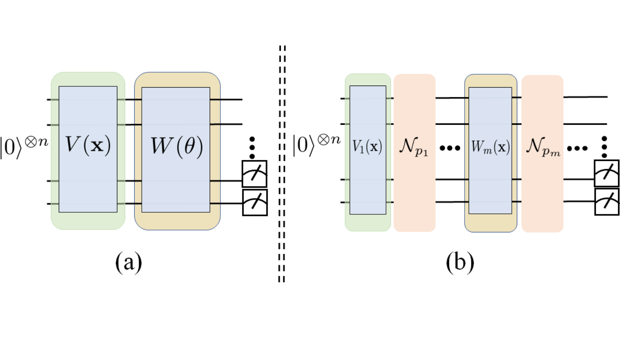
For the quantum $K$-multiclass classification task with quantum test state $\sigma$ we can employ a quantum circuit, see Fig. 1(a), to compute $\bm{\mathrm{y}}(\sigma)$ instead of using a classical circuit. We can identify $\bm{\mathrm{y}}_{k}(\sigma)$ to be the probability of the final measurement outcome of the quantum circuit being $k$,

where $\Pi_{k}$ is a POVM, $\mathcal{E}$ is a quantum operation that contains information about the trained parameters $\bm{\mathrm{\theta}}^{*}$ benedetti2019parameterized and $|a\rangle\langle a|$ is an ancilla.

However, precise values of the probabilities $\bm{\mathrm{y}}_{k}(\sigma)$ can only be obtained in the infinite sampling regime. This means that if only $N$ measurements are allowed at the output of the circuit, we can only obtain an estimated value $\bm{\mathrm{y}}^{(N)}_{k}(\sigma)$ of the output probabilities.

Adversarial examples are attacks on input examples to classification problems that lead to misclassification. In particular, these include worst-case attacks where the adversary can craft small imperceptible perturbations $\sigma\rightarrow\rho$ about a given correctly classified input $\sigma$ that result in misclassification goodfellow2014explaining. This means that while the true labels $\sigma$ and $\rho$ are identical, if $\rho$ is an adversarial example, $\mathcal{A}$ will class them differently. We can define adversarial examples more formally as follows sharif2018suitability.

If $\sigma,\rho$ are classical states, suitable distance metrics are the $l_{p}$-norms, so $h(\sigma,\rho)=||\sigma,\rho||_{p}$. If $\sigma,\rho$ are quantum states, we will use the trace distance $h(\sigma,\rho)=\tau(\sigma,\rho)=\text{Tr}(|\rho-\sigma|)/2$.

In the rest of this paper, we will use Greek letters to refer to quantum states and bold Roman letters to refer to classical states unless otherwise specified.

Differential privacy is an important concept in computer science that quantifies the sensitivity of the outputs of algorithms to changes in their input data. The less sensitive it is, the better the algorithm can preserve the privacy of the input data. Here we can formulate the definition of classical differential privacy as follows dwork2011differential.

Informally, this definition says that for two input data points separated by a small distance, a small privacy budget means that the output of the algorithm differs very little, hence the input information is partially kept private. The selection of this distance $h(\cdot,\cdot)$ varies depending on the task, e.g., Hamming distance or $l_{p}$ distance dwork2011differential. A natural distance $h(\cdot,\cdot)$ for quantum data is the trace distance, which we can employ in a definition for quantum differential privacy zhou2017differential which we will use throughout this paper. An alternative definition for quantum differential privacy aaronson2019gentle does not require quantum data $\sigma$ and $\tau$ to be close in trace distance, but rather that $\rho$ is obtainable by applying a quantum operation on only a single register of $\sigma$. See also arunachalam2020quantum for a related definition applied to PAC learning. However, for our purposes of working directly with quantum states $\sigma$ and $\rho$, the use of trace distance is the most appropriate.

Suppose $\mathcal{M}(\sigma,\Pi_{\mathcal{S}})$ is a quantum algorithm that takes input state $\sigma$, applies a quantum operation $\mathcal{E}$ before applying the POVM $\{\Pi_{k}\}$, where the set of final measurement results $k\in\mathcal{S}$. These set of outcomes are then observed with probability $\Pr(\mathcal{M}(\sigma,\Pi_{\mathcal{S}})\in\mathcal{S})=\sum_{k\in\mathcal{S}}\text{Tr}(\Pi_{k}\mathcal{E}(\mathcal{\sigma}))$. By analogy with Definition 1, we can write a definition of quantum differential privacy following Zhou and Ying zhou2017differential.

For the rest of the paper, we focus on the case $\delta=0$, which is referred to as $\epsilon$-quantum differential privacy. To illustrate a simple example, suppose we have a binary classification problem where we choose the POVM $\{\Pi_{0},\Pi_{1}=\mathbf{1}-\Pi_{0}\}$. The probability $\sigma$ is assigned class labels $k=0,1$ by a quantum binary classifier is $\tilde{\bm{\mathrm{y}}}_{0}(\sigma)\equiv\text{Tr}(\Pi_{0}(\mathcal{E}(\sigma))$ and $\tilde{\bm{\mathrm{y}}}_{1}(\sigma)=1-\tilde{\bm{\mathrm{y}}}_{0}(\sigma)$ respectively. Then if $\mathcal{M}$ satisfies $\epsilon$-quantum differential privacy, Definition 4 requires that we must satisfy

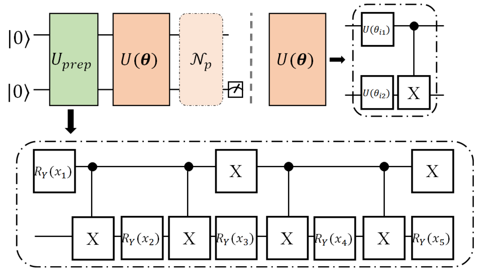
The quantum neural network (QNN), proposed by farhi2018classification, is a building block for various quantum learning models schuld2018circuit; huggins2018towards; havlivcek2019supervised; farhi2018classification; benedetti2018generative; dallaire2018quantum. The basic scheme of QNN is illustrated in Figure 2 (a), which is a special case of the circuit in Fig. 1(a). The $D$-dimensional quantum input state is $\sigma\otimes|a\rangle\langle a|$, where $\sigma$ refers to either the training or test states and $|a\rangle$ is an ancilla. The trainable unitary $U(\bm{\theta})\in\mathbb{C}^{D\times D}$ is then applied, which consists of trainable single-qubit gates and fixed two-qubit gates. Our protocol for QNN, as shown in Figure 2 (b), employs the depolarisation channels $\mathcal{N}_{p_{i}}$ that can appear within the QNN circuit before final measurements with POVM $\{\Pi_{k}\}$.

The typical application of QNN is for binary classification, broadly used in farhi2018classification; huggins2018towards; benedetti2018generative; dallaire2018quantum, where one makes single-qubit measurements using $\{\Pi_{0},\Pi_{1}=\mathbf{1}-\Pi_{0}\}$ and $D_{meas}=2$. We can apply Theorem 1 directly to our scenario and we have the following corollary.

Since $D_{meas}=2$ for binary classification, we note that the privacy budget $\epsilon$ is now independent of the dimension of the problem. Therefore, even as the feature dimension of the input $\sigma$ grows, it does not affect the robustness of the classifier against adversarial examples so long as some depolarisation noise with $0<p<1$ has been added to the circuit. This independence is an interesting contrast to the result in liu2019vulnerability which states that robustness should decrease as dimensionality of $\sigma$ grows. This contradiction is resolved by observing that, unlike in liu2019vulnerability which places no constraints on distribution from which the input states $\sigma$ are selected, here we have Eq. (12) which imposes a constraint.

In the finite sampling limit, we can employ Theorem 2 to apply to our binary classifier and we have the following corollary.

The main idea of kernel methods is to map complex input data $\bm{\mathrm{x}}$ to a higher-dimensional feature space that can then be efficiently separated goodfellow2016deep. The generic form of a quantum kernel classifier mitarai2018quantum; havlivcek2019supervised; schuld2019quantum is shown in Figure 3. The output of the kernel classifier can be written as $K(\bm{\mathrm{\theta}},\bm{\mathrm{x}})\equiv\langle 0|^{\otimes n}W(\bm{\theta})V(\bm{\mathrm{x}})|0\rangle^{\otimes n}$, where $K(\bm{\mathrm{\theta}},\bm{\mathrm{x}})$ is identified with a classical kernel with test state $\bm{\mathrm{x}}$ and weight vector captured by the trained $\bm{\mathrm{\theta}}$ values. Here $W(\bm{\theta})$ contains the trainable parameters with the aim of minimizing the predefined loss function where the optimal occurs at $\bm{\mathrm{\theta}}^{*}$ and $V(\bm{\mathrm{x}})|0\rangle^{\otimes n}$ refers to the kernel state that maps the input data into the higher-dimensional feature space. Thus the probability of obtaining the measurement values all ‘$0$’ after applying $\Pi_{0}\equiv(|0\rangle\langle 0|)^{\otimes n}$ in the noiselss circuit is given by $\bm{\mathrm{y}}_{0}(\bm{\mathrm{x}})=\langle 0|^{\otimes n}W(\bm{\mathrm{\theta}}^{*})V(\bm{\mathrm{x}})|0\rangle^{\otimes n}$.

For a binary classification problem, the class label of $\bm{\mathrm{x}}$ is $0$ if $\bm{\mathrm{y}}_{0}(\bm{\mathrm{x}})>\bm{\mathrm{y}}_{1}(\bm{\mathrm{x}})\equiv 1-\bm{\mathrm{y}}_{0}(\bm{\mathrm{x}})$. In this case, $D_{meas}=D$, thus the privacy budget becomes $\epsilon=\ln(1+D(1-p)\tau_{D}/p)$. which grows with increasing dimensionality $D$ of the input state. Corollaries 1 and 2 then hold for the quantum kernel classifier with this modified $\epsilon$.

We choose to conduct our numerical simulations on the Iris dataset fisher1936use, which has been broadly used in classical machine learning. The Iris dataset $\mathcal{D}_{I}=\{\sigma_{i},c_{i}^{*}\}_{i=1}^{150}\in\mathbb{R}^{150\times 4}\times\mathbb{R}^{150}$ consists of three different types of Iris flowers (Setosa, Versicolour, and Virginica), where examples (belonging to Setosa) with label $c^{*}_{i}=0$ are linearly separable with respect to examples (belonging to Versicolour) with label $c^{*}_{i}=1$.

Next, we remove all examples belonging to Virginica and denote the dataset that only contains label $c^{*}_{i}=0$ and $c^{*}_{i}=1$ as $\mathcal{D}$, i.e., the cardinality of $\mathcal{D}$ is $100$. Then we set the fourth entry of all examples as $0$. Afterwards, we apply $l_{2}$ normalization to each example, i.e., $\|\sigma_{i}\|_{2}=1$ for any $\sigma_{i}\in\mathcal{D}$. Then we need to efficiently encode this classical data into quantum states schuld2017implementing. We can then carry out the amplitude encoding method mottonen2004transformation to encode the normalized $\sigma_{i}$ into a quantum state.

Given the preprocessed dataset $\mathcal{D}$, we randomly split it into a training dataset $\mathcal{D}_{Tr}$ and a test dataset $\mathcal{D}_{Te}$ with $n\equiv|\mathcal{D}_{Tr}|=60$, $|\mathcal{D}_{Te}|=40$, and $\mathcal{D}=\mathcal{D}_{Tr}\cup\mathcal{D}_{Te}$. In the training procedure, we randomly sample an example $(\sigma_{i},c_{i}^{*})$ from $\mathcal{D}_{Tr}$ and forward $\sigma_{i}$ to a binary QNN classifier. For details on the circuit see Appendix H. We employ the squared loss function to train this QNN, i.e.,

where $\bar{c}_{i}=\max_{k}\bm{\mathrm{y}}_{k}(\sigma_{i})\in[0,1]$ is the score vector of QNN as formulated in Subsection II.1 and $\bm{\mathrm{y}}_{k}(\sigma)$ denotes the ideal output of the QNN.

We use the zeroth-order gradient method mitarai2018quantum to optimize trainable parameters $\bm{\theta}$ of the QNN to minimize the loss function $\mathcal{L}$. We set the number of training epochs to $50$. The learning rate is set to $0.01$ and the total number of trainable parameters is $24$. Figure 4 illustrates the training loss, training accuracy and test accuracy. Both the training and test accuracy converges to $100\%$ after $15$ epochs (See Appendix H for more implementation details). Given the test dataset $\mathcal{D}_{Te}$, we randomly select three test examples and explore how the maximum robustness $\tau_{D}$ changes with varied $p$ according to Eq. (11), which we can rewrite as

Figure 5 illustrates how $\tau_{D}$ scales with different $p$ for three different test examples with $D_{meas}=2$. Note that the constants $\epsilon$ are different for the three test examples and the test examples satisfy the condition in Eq. (12). In the same figure, we also plot how the test score $\tilde{\bm{\mathrm{y}}}_{0}(\sigma)$ varies with $p$, coming from Eq. (10) for the case of binary classification $K=2$

To evaluate the performance of our protocol, we adopt an adversarial attack method that is widely employed in classical machine learning. It is known as the iterative-fast gradient sign method (I-FGSM) with $l_{2}$-bounded norm liu2016delving; dong2018boosting; madry2018towards that aims to attack the test dataset $\mathcal{D}_{\text{Te}}$ to make incorrect predictions when using a trained classifier. If we denote the original input by $\bm{\mathrm{x}}$ and the adversarial example at the $t^{\text{th}}$ updating step when using the I-FGSM by $\bm{\mathrm{x}}^{\prime}(t)$, then

where $\alpha=L/T$ is the learning rate with $\|\bm{\mathrm{x}}-\bm{\mathrm{x}}^{\prime}\|_{2}\leq L$ and $\mathcal{L}$ is the loss function formulated in Eq. (14).

Here we employ our trained classifier and the adversarial attack method formulated above to quantify the performance of our protocol. Recall that Corollaries 1 and 2 are the special cases of Theorems 1 and 2 when applied to binary QNN classifiers and work in the regime of using infinite and finite sampling of the output probabilities respectively. Here we explore how our protocol protects the binary QNN classifier against adversarial attacks under these two settings.

The infinite sampling case. At testing time, we randomly sample an example $(\rho=|\bm{\mathrm{x}}\rangle\langle\bm{\mathrm{x}}|,\tilde{y})$ from $\mathcal{D}_{Te}$ to investigate its robustness $\tau_{D}$ with respect to different level of depolarisation noise $p$. Without loss of generality, the original test example has label $\tilde{y}=0$. We set three different values of $p$ and $\tau_{D}$: $\{p^{(1)}=0.5,\tau_{D}^{(1)}=0.02\}$; $\{p^{(2)}=0.1,\tau_{D}^{(1)}=0.02\}$ and $\{p^{(1)}=0.5,\tau_{D}^{(2)}=0.2\}$. From Eq. (11), their corresponding privacy budgets are $\epsilon_{1}=1.04$, $\epsilon_{2}=1.36$ and $\epsilon_{3}=1.4$. Given our input $\rho$, the outputs of our trained classifier with added depolarizsation noise are $\Pr(\tilde{\bm{\mathrm{y}}}^{(1)}(\rho)=0)=54.46\%$, $\Pr(\tilde{\bm{\mathrm{y}}}^{(2)}(\rho)=0)=58.04\%$ and $\Pr(\tilde{\bm{\mathrm{y}}}^{(3)}(\rho)=0)=54.46\%$, where the corresponding constants $B$ defined in Corollary 1 is $B^{(1)}=1.20$, $B^{(2)}=1.38$, and $B^{(3)}=1.20$, respectively. Following the condition for robustness in Eq. (12), we have confidence that the classifier is robust to adversarial attacks if $B>e^{2\epsilon}$. A simple comparison indicates that robustness is guaranteed when $\{p=0.5,\tau_{D}=0.02\}$, since $B^{(1)}>e^{2\epsilon_{1}}=1.08$ while $B^{(2)}<e^{2\epsilon_{2}}=1.85$ and $B^{(3)}<e^{2\epsilon_{3}}=1.96$.

To validate the correctness of our theoretical results, we employ I-FGSM to attack our trained classifier, where we identify the $l_{2}$-norm bound with its corresponding $\tau_{D}$ value. The left panel of Figure 6 demonstrates the simulation results and Table 1 shows the final test score of the attacked input. The classifier with the first setting $\{p^{(1)}=0.5,\tau_{D}^{(1)}=0.02\}$ is robust to the bounded-norm adversarial attacks, where the predicted label of $\tilde{\bm{x}}$ is still ‘0’. For the third setting when $\{p^{(3)}=0.5,\tau_{D}^{(3)}=0.2\}$, the adversary can easily perturb the input and lead the classifier to give the wrong prediction. In particular, the adversary can easily perturb the input to cross the classification boundary, as highlighted by the purple line. For the second setting with $\{p^{(2)}=0.1,\tau_{D}^{(2)}=0.05\}$, the classifier correctly predicts the label, while our protocol cannot provide any promises, since Theorem 1 and Corollary 1 provides only sufficient conditions for robustness. The above three simulation results are then in accordance with our theoretical results.

The finite sampling case. The only difference in the finite sampling case is the acquisition of the output of our trained classifier. The same test example $(\rho=|\bm{\mathrm{x}}\rangle\langle\bm{\mathrm{x}}|,\tilde{y})$ is employed. The hyperparameters are set as $\{p^{(1)}=0.5,\tau_{D}^{(1)}=0.02\}$ and from Eq. (11), the privacy budget $\epsilon=1.04$ is fixed. We set three different sampling number values $n_{samp}$ to explore how $n_{samp}$ affects the robustness guarantees, where $n_{samp}^{(1)}=50$, $n_{samp}^{(2)}=500$, and $n_{samp}^{(3)}=5000$. The corresponding three approximated test scores are $\Pr(\tilde{\bm{\mathrm{y}}}^{(1)}=0)=0.515$, $\Pr(\tilde{\bm{\mathrm{y}}}^{(2)}=0)=0.529$ and $\Pr(\tilde{\bm{\mathrm{y}}}^{(3)}=0)=0.552$. The corresponding parameters $B$ are $B^{(1)}=1.06$, $B^{(2)}=1.124$, and $B^{(3)}=1.23$ with respect to $n_{samp}^{(1)}$, $n_{samp}^{(2)}$, and $n_{samp}^{(3)}$. Following the results of Theorem 2 and Corollary 2, with probability at least $1-2\exp\left(-{2n_{samp}\zeta^{2}}\right)$, the trained classifier with added depolarisation noise is robust to adversarial attacks if ${B}>e^{2\epsilon}$. By setting $\zeta=0.95$, a simple inspection shows that $n_{samp}=5000$ guarantees robustness. Analogous to the infinite sampling case, we employ a bounded-norm adversary to confirm the correctness of our theory result, where the simulation results are shown in the right panel of Figure 6.

For more details on the implementation of the classifier and perfomance analysis of our protocol please see Appendix H.

While in the quantum case the theoretical bound on robustness is independent of the details of the classification model and is simple to compute, this is not true in the best known classical protocol. Before elaborating on this quantum advantage, we briefly review the classical results.

Following the results of lecuyer2019certified, classical $\epsilon$-differential privacy of a classification algorithm is obtained by adding noise sampled from the Laplacian distribution $\mathcal{N}(\bm{z},\kappa)$ to the trained classifier. This is commonly known as the Laplace mechanism. For numerical functions ³³ 3 For non-numerical functions, the exponential mechanism is employed., the only other common method to attain differential privacy is the Gaussian mechanism, which adds noise sampled from the Gaussian distribution. However, this leads to classical $(\epsilon,\delta)$-differential privacy where $\delta\neq 0$, so cannot be directly compared to our quantum scenario where $\delta=0$. The Laplacian distribution used in the Laplace mechanism can be written as

where $\kappa$ refers to the variance of the Laplacian distribution and $L$ is the upper-bounded $l_{2}$ norm between original input $\bm{\mathrm{x}}$ and attacked input $\bm{\mathrm{x}}^{\prime}$ such that classical $\epsilon$-differential privacy is preserved. The sensitivity $\Delta f$ of the function $f(\cdot)$ applied at a layer of the neural network classifier just before the Laplacian noise is injected is defined as

The classical protocol runs in the following way. In the testing phase, the adversarial example $\bm{\mathrm{x}}^{\prime}$, where $\|\bm{\mathrm{x}}-\bm{\mathrm{x}}^{\prime}\|_{2}\leq L$ and $\bm{\mathrm{x}}$ is the original test example, is inserted into the trained classifier $\bm{\mathrm{y}}(\cdot)$. The predicted label for $\bm{\mathrm{x}}^{\prime}$ is obtained by invoking $\bm{\mathrm{y}}(\bm{\mathrm{x}}^{\prime})$ a total $N$ times. For every run of $\bm{\mathrm{y}}(\bm{\mathrm{x}}^{\prime})$, the noise $z_{i,j}$ with $i=1,...,N$ is independently sampled from $\mathcal{N}_{L}(\bm{z},\kappa)$ and applied to the input to some layer $j$ of the neural network realising the classifier. Let $N_{k}$ denote the number of times that the predicted label is $k$, so the probability of the predicted label being $k$ is given by $N_{k}/N$. Then, similarly to Theorem 2, we can write the following condition for robustness of the $K$-class classifier under the Laplace mechanism.

This means that this best available classical theoretical bound to $L$ depends on $\Delta f$, which in general is dependent on both the details of the classification model used and the layer of the neural network in which the Laplacian noise is injected. However, in the quantum scenario with depolarisation noise, we see that the robustness bound is independent of both $U$, the circuit realising the quantum classifier, as well as the location or locations of noise injection. This means that the adversarial robustness bound is universal for all quantum classifiers.

We can see this from the fact that the final state of the quantum circuit after applying depolarisation noise in layers $1$ to $l$ depends only on the product $\prod_{i=1}^{l}(1-p_{i})$, which is independent of $U$ and invariant under any re-ordering of the layers. This simplicity in the quantum case results from two facts: that the ‘noisy’ part of depolarisation noise lies in injecting a maximally-mixed channel with a certain probability and that unitary $U$ operations realising any quantum classifier are unital (i.e., the identity operator $\mathbf{1}$ remains invariant under $U$). On the other hand, there is no known classical equivalent of this property that also gives rise to differential privacy.

The dependence of $\Delta f$ on the details of the classifier in the most general cases also leads to a difficulty in the computation of $\Delta f$ and is often intractable except in the simplest cases lecuyer2019certified. This means that, unlike in the quantum case, the corresponding classical bound on robustness $L$ cannot be derived in closed form from Eq. (20) in the most general case.

However, in special simple cases we can provide quantitative examples of this quantum advantage. As a simple illustration, we can look at the binary classifier for the kernel perceptron, which can be written as

where $\{(\bm{\mathrm{x}}_{i}^{*},y^{*}_{i})\}_{i=1}^{M}$ are the $M$ training examples and $\{w_{i}^{*}\}_{i=1}^{M}$ are trained parameters of the classifier. We can consider the polynomial kernel

where $n$ is the kernel degree and $n=1$ is the special case of the linear kernel. We now have the following theorem.

From this we see that we can guarantee only a smaller robustness bound for a more nonlinear kernel (i.e., higher $n$). We can also use a quantum classifier below to realise the same polynomial kernel and find a robustness bound that is now independent of degree of nonlinearity of the kernel.

References

- [1] Scott Aaronson and Guy N Rothblum. Gentle measurement of quantum states and differential privacy. arXiv:1904.08747, 2019.
- [2] Srinivasan Arunachalam, Alex B Grilo, and Henry Yuen. Quantum statistical query learning. arXiv:2002.08240, 2020.
- [3] Marcello Benedetti, Delfina Garcia-Pintos, Oscar Perdomo, Vicente Leyton-Ortega, Yunseong Nam, and Alejandro Perdomo-Ortiz. A generative modeling approach for benchmarking and training shallow quantum circuits. npj Quantum Information, 5(1):1–9, 2019.
- [4] Marcello Benedetti, Erika Lloyd, Stefan Sack, and Mattia Fiorentini. Parameterized quantum circuits as machine learning models. Quantum Science and Technology, 4(4):043001, 2019.
- [5] Jacob Biamonte, Peter Wittek, Nicola Pancotti, Patrick Rebentrost, Nathan Wiebe, and Seth Lloyd. Quantum machine learning. Nature, 549(7671):195, 2017.
- [6] Pierre-Luc Dallaire-Demers and Nathan Killoran. Quantum generative adversarial networks. Physical Review A, 98(1):012324, 2018.
- [7] Yinpeng Dong, Fangzhou Liao, Tianyu Pang, Hang Su, Jun Zhu, Xiaolin Hu, and Jianguo Li. Boosting adversarial attacks with momentum. In Proceedings of the IEEE conference on computer vision and pattern recognition, pages 9185–9193, 2018.
- [8] Cynthia Dwork. Differential privacy. Encyclopedia of Cryptography and Security, pages 338–340, 2011.
- [9] Suguru Endo, Simon C Benjamin, and Ying Li. Practical quantum error mitigation for near-future applications. Physical Review X, 8(3):031027, 2018.
- [10] Edward Farhi and Hartmut Neven. Classification with quantum neural networks on near term processors. arXiv:1802.06002, 2018.
- [11] Ronald A Fisher. The use of multiple measurements in taxonomic problems. Annals of Eugenics, 7(2):179–188, 1936.
- [12] Luca Gammaitoni, Peter Hänggi, Peter Jung, and Fabio Marchesoni. Stochastic resonance. Reviews of modern physics, 70(1):223, 1998.
- [13] Ian Goodfellow, Yoshua Bengio, and Aaron Courville. Deep learning. MIT press, 2016.
- [14] Ian Goodfellow, Patrick McDaniel, and Nicolas Papernot. Making machine learning robust against adversarial inputs. Communications of the ACM, 61(7), 2018.
- [15] Ian J Goodfellow, Jonathon Shlens, and Christian Szegedy. Explaining and harnessing adversarial examples. arXiv:1412.6572, 2014.
- [16] Edward Grant, Marcello Benedetti, Shuxiang Cao, Andrew Hallam, Joshua Lockhart, Vid Stojevic, Andrew G Green, and Simone Severini. Hierarchical quantum classifiers. npj Quantum Information, 4(1):1–8, 2018.
- [17] Vojtěch Havlíček, Antonio D Córcoles, Kristan Temme, Aram W Harrow, Abhinav Kandala, Jerry M Chow, and Jay M Gambetta. Supervised learning with quantum-enhanced feature spaces. Nature, 567(7747):209, 2019.
- [18] Ling Huang, Anthony D Joseph, Blaine Nelson, Benjamin IP Rubinstein, and J Doug Tygar. Adversarial machine learning. In Proceedings of the 4th ACM workshop on Security and artificial intelligence, pages 43–58. ACM, 2011.
- [19] William Huggins, Piyush Patil, Bradley Mitchell, K Birgitta Whaley, and Miles Stoudenmire. Towards quantum machine learning with tensor networks. Quantum Science and Technology, 4(2):024001, 2019.
- [20] Kam Jim, Bill G Horne, and C Lee Giles. Effects of noise on convergence and generalization in recurrent networks. In Advances in neural information processing systems, pages 649–656, 1995.
- [21] Alexey Kurakin, Ian Goodfellow, and Samy Bengio. Adversarial machine learning at scale. arXiv:1611.01236, 2016.
- [22] Ryan LaRose and Brian Coyle. Robust data encodings for quantum classifiers. arXiv:2003.01695, 2020.
- [23] Mathias Lecuyer, Vaggelis Atlidakis, Roxana Geambasu, Daniel Hsu, and Suman Jana. Certified robustness to adversarial examples with differential privacy. In 2019 IEEE Symposium on Security and Privacy (SP), pages 656–672. IEEE, 2019.
- [24] Nana Liu and Peter Wittek. Vulnerability of quantum classification to adversarial perturbations. arXiv: 1905.04286, 2019.
- [25] Yanpei Liu, Xinyun Chen, Chang Liu, and Dawn Song. Delving into transferable adversarial examples and black-box attacks. arXiv:1611.02770, 2016.
- [26] Sirui Lu, Lu-Ming Duan, and Dong-Ling Deng. Quantum adversarial machine learning. arXiv:2001.00030, 2019.
- [27] Aleksander Madry, Aleksandar Makelov, Ludwig Schmidt, Dimitris Tsipras, and Adrian Vladu. Towards deep learning models resistant to adversarial attacks. arXiv:1706.06083, 2017.
- [28] Kosuke Mitarai, Makoto Negoro, Masahiro Kitagawa, and Keisuke Fujii. Quantum circuit learning. Physical Review A, 98(3):032309, 2018.
- [29] Mehryar Mohri, Afshin Rostamizadeh, and Ameet Talwalkar. Foundations of machine learning. MIT press, 2018.
- [30] Mikko Mottonen, Juha J Vartiainen, Ville Bergholm, and Martti M Salomaa. Transformation of quantum states using uniformly controlled rotations. arXiv: quant-ph/0407010, 2004.
- [31] Michael A Nielsen and Isaac L Chuang. Quantum computation and quantum information. Cambridge University Press, 2010.
- [32] Martin Plesch and Časlav Brukner. Quantum-state preparation with universal gate decompositions. Physical Review A, 83(3):032302, 2011.
- [33] John Preskill. Quantum computing in the nisq era and beyond. arXiv:1801.00862, 2018.
- [34] Lawrence Roberts. Picture coding using pseudo-random noise. IRE Transactions on Information Theory, 8(2):145–154, 1962.
- [35] Maria Schuld, Alex Bocharov, Krysta Svore, and Nathan Wiebe. Circuit-centric quantum classifiers. arXiv:1804.00633, 2018.
- [36] Maria Schuld, Mark Fingerhuth, and Francesco Petruccione. Implementing a distance-based classifier with a quantum interference circuit. EPL (Europhysics Letters), 119:60002, 2017.
- [37] Maria Schuld and Nathan Killoran. Quantum machine learning in feature hilbert spaces. Physical Review Letters, 122(4):040504, 2019.
- [38] Mahmood Sharif, Lujo Bauer, and Michael K Reiter. On the suitability of lp-norms for creating and preventing adversarial examples. In Proceedings of the IEEE Conference on Computer Vision and Pattern Recognition Workshops, pages 1605–1613, 2018.
- [39] Christian Szegedy, Wojciech Zaremba, Ilya Sutskever, Joan Bruna, Dumitru Erhan, Ian Goodfellow, and Rob Fergus. Intriguing properties of neural networks. arXiv:1312.6199, 2013.
- [40] Kristan Temme, Sergey Bravyi, and Jay M Gambetta. Error mitigation for short-depth quantum circuits. Physical Review Letters, 119(18):180509, 2017.
- [41] Nathan Wiebe and Ram Shankar Siva Kumar. Hardening quantum machine learning against adversaries. New Journal of Physics, 20(12):123019, 2018.
- [42] Eric Wong and Zico Kolter. Provable defenses against adversarial examples via the convex outer adversarial polytope. In International Conference on Machine Learning, pages 5283–5292, 2018.
- [43] Xiaoyong Yuan, Pan He, Qile Zhu, and Xiaolin Li. Adversarial examples: Attacks and defenses for deep learning. IEEE transactions on neural networks and learning systems, 30(9):2805–2824, 2019.
- [44] Li Zhou and Mingsheng Ying. Differential privacy in quantum computation. In 2017 IEEE 30th Computer Security Foundations Symposium (CSF), pages 249–262. IEEE, 2017.
Appendix A Proof of Lemma 1
Here we prove that if the noiseless quantum classifier assigns to the class , i.e., , then the noisy circuit with depolarisation noise also assigns to the class , i.e. . This is equivalent to the condition that if , then .
Appendix B Proof of Proposition 1
From Lemma 1, we know that if is labelled as in the noiseless circuit then in the infinite sampling limit this label is maintained in the corresponding circuit with depolarisation noise, so . However, in the finite sampling limit with sample complexity , we only have access to the estimate . So we want to find the smallest so with probability at least .
From results in Lemma 1, we see that since and , then . Thus we need large enough sampling to resolve the difference to at least . It is then sufficient to find that estimates to precision . To find , we can employ Hoeffding’s inequality in the following.
Lemma A. (Hoeffding’s inequality [29])
Let be independent bounded random variables with for all , where . Then the probability