Sequential Bayesian Experimental Design for Implicit Models via Mutual Information

In Bayesian experimental design the aim is to find experimental designs $\mathbf{d}$ that yield more informative, or useful, real-world observations than others. Furthermore, in this work we are particularly interested in finding the optimal design $\mathbf{d}^{\ast}$ that results in the best estimation of the model parameters. At its core, this task requires defining a utility function $U(\mathbf{d})$ that describes the value of performing an experiment at $\mathbf{d}\in\mathcal{D}$, where $\mathcal{D}$ defines the space of possible designs. In order to qualify as a ‘fully Bayesian design’, this utility has to be a functional of the posterior distribution $p(\bm{\theta}\mid\mathbf{d},\mathbf{y})$ (Ryan et al. 2016), where $\bm{\theta}$ are the model parameters and $\mathbf{y}$ is simulated data. The utility function is then maximised in order to find the optimal design $\mathbf{d}^{\ast}$, i.e.

The choice of utility function $U(\mathbf{d})$ is thus critical, as different functions will usually lead to different optimal designs. The most suitable utilities naturally depend on the task in question, but there are a few common functions that have been used extensively in the literature. For instance, the Bayesian D-Optimality (BD-Opt) is based on the determinant of the inverse covariance matrix of the posterior distribution,¹¹ 1 See the Appendix A for an alternative form of the BD-Opt utility. and is a measure of how precise the resulting posterior might be given certain designs (Ryan et al. 2016),

While BD-Opt works well for uni-modal posteriors, it is not suitable for multi-modal or complex posteriors as it heavily penalises diversion from uni-modality. A more versatile and robust utility function is the mutual information, one of the most principled choices in Bayesian experimental design (Ryan et al. 2016 e.g.).

The mutual information $\mathrm{I}(\bm{\theta};\mathbf{y}|\mathbf{d})$ can be interpreted as the expected reduction in uncertainty (entropy) of the model parameters if the data $\mathbf{y}$ was obtained with design $\mathbf{d}$. It accounts for possibly non-linear dependencies between $\bm{\theta}$ and $\mathbf{y}$. It is an effective metric with regards to the task of parameter estimation, as we are essentially concerned with finding the design for which the corresponding observation yields the most information about the model parameters $\bm{\theta}$. In other words, mutual information tells us how ‘much’ we can learn about the model parameters given the prospective data at a particular design.

Mutual information is defined as the Kullback-Leibler (KL) divergence $\mathrm{D_{KL}}$ (Kullback and Leibler 1951) between the joint distribution and the product of marginal distributions of $\mathbf{y}$ and $\bm{\theta}$ given $\mathbf{d}$, i.e.

where we have made the usual assumption that our prior belief about $\bm{\theta}$ is not affected by the design, i.e. $p(\bm{\theta}\mid\mathbf{d})$ = $p(\bm{\theta})$.

The mutual information can also be interpreted as the expected KL divergence between posterior $p(\bm{\theta}\mid\mathbf{d},\mathbf{y})$ and prior $p(\bm{\theta})$ (Ryan et al. 2016 see e.g.) and essentially tells us how different on average our posterior distribution is to the prior distribution. The utility that we then need to maximise in order to find the optimal design $\mathbf{d}^{\ast}$ is thus

where $p(\mathbf{y}\!\mid\!\bm{\theta},\mathbf{d})$ is the data generating distribution, commonly referred to as the likelihood. The particular form of mutual information in (2.8) can be obtained from (2.5) by applying the product rule to $p(\bm{\theta},\mathbf{y}\!\mid\!\mathbf{d})$. Even though mutual information is a well-studied concept, estimating it efficiently remains an open question, especially in higher dimensions.

Assuming for now that we have optimised the utility function in (2.8) and have obtained the optimal design $\mathbf{d}^{\ast}$. An experimenter would then go and perform the experiment at $\mathbf{d}^{\ast}$ and observe real-world data $\mathbf{y}^{\ast}$. Everything up to this point is $\emph{static}$ Bayesian experimental design. If we would like to update our optimal design in light of a real-world observation, we would have to perform $\emph{sequential}$ Bayesian experimental design, i.e. update our prior distribution and optimise the utility function again. This procedure is then repeated several times to obtain (myopic) sequentially designed experiments. We shall not aim to find non-myopic sequentially designed experiments where we would we plan ahead more than one time-step as this adds another layer of complexity.

Let $k$ be the $k$th iteration of the sequential design procedure, where $k=1$ corresponds to the task of finding the first optimal experimental design $\mathbf{d}^{\ast}_{1}$ yielding real-world observation $\mathbf{y}^{\ast}_{1}$. At iteration $k$ we then optimise the utility function $U_{k}(\mathbf{d})$ to obtain sequential optimal designs $\mathbf{d}_{k}^{\ast}$, with corresponding real-world observations $\mathbf{y}_{k}^{\ast}$. The utility function at iteration $k\in\{1,2,\ldots,K\}$ depends on the set of all previous observations $\mathbb{D}_{k-1}=\{\mathbf{d}^{\ast}_{1:k-1},\mathbf{y}^{\ast}_{1:k-1}\}$, with $\mathbb{D}_{0}=\varnothing$, and therefore will change at every iteration. Its form stays similar to (2.8), except that the prior and posterior distributions now depend on $\mathbb{D}_{k-1}$, i.e.

Note that we will assume that data is generated independently of previous observations, i.e. $p(\mathbf{y}\mid\bm{\theta},\mathbf{d},\mathbb{D}_{k-1})=p(\mathbf{y}\mid\bm{\theta},\mathbf{d})$. In certain special cases where gathering real-world observations changes the data-generating process this would not be the case.

Implicit models have intractable likelihood functions, which means that $p(\mathbf{y}\mid\bm{\theta},\mathbf{d})$ is either too expensive to compute or there is no closed-form expression. This results in standard Bayesian inference becoming infeasible. Because of their widespread use however, it is crucial to be able to infer the parameters of implicit models. As a result, the field of likelihood-free inference has emerged. These methods leverage the fact that, by definition, implicit models allow for sampling from the data-generating distribution.

A popular likelihood-free approach is Approximate Bayesian Computation (Rubin 1984 ABC,). ABC rejection sampling (Pritchard et al. 1999), the simplest form of ABC, works by generating samples from the prior distribution over the model parameters and then using them to simulate data from the implicit model. The prior parameters that result in data that is ‘close’ to observed data are then accepted as samples from the ABC posterior distribution. See Sisson et al. 2018 or Lintusaari et al. 2017 for reviews on ABC.

Since standard ABC is notoriously slow and requires tuning of some hyperparameters, there has been considerable research in making likelihood-free inference more efficient, using, for example, ideas from Bayesian optimisation and experimental design (Gutmann and Corander 2016; Järvenpää et al. 2019; Järvenpää et al. 2020), conditional density estimation (Papamakarios and Murray 2016; Lueckmann et al. 2017; Greenberg et al. 2019), classification (Gutmann et al. 2018), indirect inference (Drovandi et al. 2015), optimisation (Meeds and Welling 2015; Ikonomov and Gutmann 2020), and more broadly surrogate modelling with Gaussian processes (Wilkinson 2014; Meeds and Welling 2015) and neural networks (Blum and Francois 2010; Chen and Gutmann 2019; Papamakarios et al. 2019).

In this paper, we make use of another approach to likelihood-free inference called Likelihood-Free Inference by Ratio Estimation (LFIRE) (Thomas et al. 2016). LFIRE uses density ratio estimation to obtain ratios $r(\mathbf{d},\mathbf{y},\bm{\theta})$ of the likelihood to marginal density and, therefore, the posterior to prior density, i.e.

The method works by estimating the ratio from data simulated from the likelihood $p(\mathbf{y}\mid\bm{\theta},\mathbf{d})$ and data simulated from the marginal $p(\mathbf{y}\mid\mathbf{d})$, e.g. via logistic regression (Thomas et al. 2016). Since the prior density $p(\bm{\theta})$ is known, learning the ratio corresponds to learning the posterior, i.e. $\widehat{p}(\bm{\theta}\mid\mathbf{d},\mathbf{y})=\widehat{r}(\mathbf{d},\mathbf{y},\bm{\theta})p(\bm{\theta})$. Importantly, the learned ratio yields automatically also an estimate of the mutual information in (2.9).

The LFIRE framework can be used with arbitrary models of the ratio or posterior. For simplicity, like in the simulations by Thomas et al. 2016, we here use the log-linear model

where $\bm{\psi}(\mathbf{y})$ are some fixed summary statistics. Thomas et al. 2016 showed that this log-linear model, while simple, generalises the popular synthetic likelihood approach by Wood 2010; Price et al. 2018b. Moreover, learning the summary statistics from data, e.g. by means of neural networks, is possible too (Dinev and Gutmann 2018). For further details on LFIRE, we refer the reader to the original paper by Thomas et al. 2016.

We assume that we have already made $k-1$ experiments resulting in the set of optimal designs and observations $\mathbb{D}_{k-1}=\{\mathbf{d}^{\ast}_{1:k-1},\mathbf{y}^{\ast}_{1:k-1}\}$, with $\mathbb{D}_{0}=\varnothing$. At iteration $k$ of the sequential BED procedure we then set out to determine the optimal design $\mathbf{d}^{\ast}_{k}$ and the corresponding real-world observation $\mathbf{y}^{\ast}_{k}$. To do so, we first approximate the density ratio of $p(\bm{\theta}\mid\mathbf{d},\mathbf{y},\mathbb{D}_{k-1})$ and $p(\bm{\theta}\mid\mathbb{D}_{k-1})$ by the ratio $\widehat{r}_{k}(\mathbf{d},\mathbf{y},\bm{\theta},\mathbb{D}_{k-1})$ computed by LFIRE,²² 2 Note that LFIRE actually estimates the log ratio of posterior to prior density. such that

We then plug this into the expression for the sequential MI utility in (2.9) and obtain

We can approximate this with a Monte-Carlo sample average to obtain the estimate

where $\mathbf{y}^{(i)}\sim p(\mathbf{y}\mid\mathbf{d},\bm{\theta}^{(i)})$ and $\bm{\theta}^{(i)}\sim p(\bm{\theta}\mid\mathbb{D}_{k-1})$. The above mutual information estimate $\widehat{U}_{k}(\mathbf{d})$ is then optimised to find the optimal design $\mathbf{d}_{k}^{\ast}$ and, through a real-world experiment, the corresponding observation $\mathbf{y}_{k}^{\ast}$ at iteration $k$.

Two core technical difficulties in (3.4) are (1) how to obtain parameter samples $\bm{\theta}^{(i)}\sim p(\bm{\theta}\mid\mathbb{D}_{k-1})$ from the updated belief distribution and (2) how to compute the sequential LFIRE ratio in (3.1) given the observations $\mathbb{D}_{k-1}$. We explain our solutions to these difficulties in Sections 3.2 to 3.4.

For iteration $k=1$ we only require samples from the prior distribution $p(\bm{\theta})$ in order to compute the MI in (3.4). We here assume that sampling from the prior is possible. For iteration $k=2$, we require samples from $p(\bm{\theta}\mid\mathbb{D}_{1})$, for $k=3$ we require samples from $p(\bm{\theta}\mid\mathbb{D}_{2})$, etc. We here describe how to obtain samples from the updated belief $p(\bm{\theta}\mid\mathbb{D}_{k})$ after any iteration $k$. For that, let us first define what it means to update the belief about the model parameters. After observing real-word data $\mathbf{y}^{\ast}_{k}$ at optimal design $\mathbf{d}^{\ast}_{k}$, we update the observation data set, i.e. $\mathbb{D}_{k}=\mathbb{D}_{k-1}\cup\{\mathbf{d}_{k}^{\ast},\mathbf{y}^{\ast}_{k}\}$. For $\mathbf{d}=\mathbf{d}^{\ast}_{k}$ and $\mathbf{y}=\mathbf{y}^{\ast}_{k}$, the numerator in (3.1) equals $p(\bm{\theta}\mid\mathbb{D}_{k})$, leading us to an expression for the updated belief distribution,

Furthermore, we can approximate the belief distribution $p(\bm{\theta}\mid\mathbb{D}_{k})$ after iteration $k$ as a product of $k$ estimated density ratios and the initial prior $p(\bm{\theta})$,

Each of the density ratios $\widehat{r}_{s}$ in (3.6) are evaluated at the observations $\{\mathbf{d}_{s}^{\ast},\mathbf{y}_{s}^{\ast}\}$ of the relevant iteration $s$, but also depend on all previous observations $\mathbb{D}_{s-1}$. We can write this product of density ratios as a weight function $w_{k}$ and then (3.6) becomes

where we have defined the weight function $w_{k}$ to be

with $\widehat{r}_{1}(\mathbf{d}_{1}^{\ast},\mathbf{y}_{1}^{\ast},\bm{\theta},\mathbb{D}_{0})=\widehat{r}_{1}(\mathbf{d}_{1}^{\ast},\mathbf{y}_{1}^{\ast},\bm{\theta})$ according to (2.10) and $w_{0}(\bm{\theta})=1\,\forall\,\bm{\theta}$.

We use the weight function in (3.8) to obtain samples from the updated belief distribution $p(\bm{\theta}\mid\mathbb{D}_{k})$. To do so, we first sample $N$ initial prior samples $\bm{\theta}^{(i)}\sim p(\bm{\theta})$. After every iteration $k$ we then obtain weights $w_{k}^{(i)}=w_{k}(\bm{\theta}^{(i)};\mathbb{D}_{k})$ corresponding to the initial prior samples, which form a particle set $\{w_{k}^{(i)},\bm{\theta}^{(i)}\}_{i=1}^{i=N}$. We compute these by updating each weight $w_{k-1}^{(i)}$ by the LFIRE ratio evaluated at the observed data according to (3.8), in order to yield $w_{k}^{(i)}$. Since we can store the weights $w_{k-1}^{(i)}$ for a particular parameter, we do not need to recompute them.

To finally obtain updated belief samples, we first normalise the weights: $W_{k}^{(i)}=w_{k}^{(i)}/\,\Sigma_{i=1}^{N}w_{k}^{(i)}$. Then we sample an index from the categorical distribution, i.e. $I\sim\text{cat}(\{W_{k}^{(i)}\})$, and choose the initial prior sample $\bm{\theta}^{(I)}$. Repeating this several times results in a set of parameter samples that follows $p(\bm{\theta}\mid\mathbb{D}_{k})$. We have summarised this procedure in Algorithm 1.

We note that approximating (3.3) directly with weighted samples from $p(\bm{\theta})$ instead of using Algorithm 1 to obtain samples from $p(\bm{\theta}\mid\mathbb{D}_{k-1})$ would theoretically result in a lower variance Monte-Carlo estimator. However, because we did not observe this in our simulations and Algorithm 1 had lower computation times, we opted to use Algorithm 1 instead. For more details see Appendix B.

We can see from (3.8) that a weight $w_{k}^{(i)}$ is computed by the product of LFIRE ratios given all previous observations. Less significant parameter samples, i.e. ones with a low density ratio, thus have weights that quickly decay to zero. This means that after several iterations we may be left with only a few weights $w_{k}^{(i)}$ that are effectively non-zero. Eventually, only few different parameter samples $\bm{\theta}^{(i)}$ of the current particle set are chosen in the sampling scheme in Algorithm 1, which increases the Monte-Carlo error of the sequential utility in (3.4) and of the marginal samples in the sequential LFIRE procedure (see Section 3.4).

We can quantify how many effective samples we have via the effective sample size $\eta$ (Kish 1965),

If $\eta$ is small, i.e. $\eta\ll N$, then they do not cover much relevant parameter space and our Monte-Carlo approximations may become poor. Thus, if the effective sample size becomes smaller than a minimum sample size $\eta_{\text{min}}$ we need to resample our set of parameter samples; this allows us to have a set of new parameter samples that well-represent the current belief distribution. From a practical point of view, throughout this work we shall use the typical value of $\eta_{\text{min}}=N/2$ (Chen 2003; Doucet and Johansen 2009 e.g.).

We start the resampling procedure by transforming the parameter space such that all parameter samples $\bm{\theta}^{(i)}$ have values between $0$ and $1$, i.e. $\bm{\theta}\rightarrow\bm{\theta}^{\prime}$. This ensures that different parameter dimensions have similar scales, thereby increasing the robustness of the following steps.³³ 3 See Appendix C for a more detailed explanation. If the parameter space has boundary conditions $\mathcal{B}$, through a bounded prior distribution for instance, then we transform these in the same way as the parameter space, $\mathcal{B}\rightarrow\mathcal{B}^{\prime}$ (see Appendix C). In this transformed space, we model the belief distribution $p(\bm{\theta}^{\prime}\mid\mathbb{D}_{k})$ after the current iteration $k$ as a truncated Mixture of Gaussians (MoG), i.e.

where $\mathbb{I}$ is the identity matrix, $\sigma^{2}$ is a variance parameter and $W_{k}^{(i)}$ are the normalised weights. The indicator function $\mathds{1}_{\mathcal{B}^{\prime}}(\bm{\theta}^{\prime})$ is $1$ if $\bm{\theta}^{\prime}$ satisfies the boundary conditions $\mathcal{B}^{\prime}$ and $0$ otherwise. Note that we have one Gaussian for every parameter sample of the current particle set; each Gaussian is centred at that parameter sample $\bm{\theta}^{\prime(i)}$ and has the same standard deviation $\sigma$. The parameter $\sigma$ is typically small which means that (3.10) should be understood more in terms of smoothing than Gaussian mixture modelling.

We compute the Gaussian standard deviation by first using a k-dimensional (KD) tree (Bentley 1975) to find the nearest neighbour $\text{NN}(\bm{\theta}^{\prime(i)})$ of each parameter sample. Let $\delta$ be the median of all the distances of a sample to its nearest neighbour, i.e. $\delta=\text{median}\left(\lvert\bm{\theta}^{\prime(i)}-\text{NN}(\bm{\theta}^{\prime(i)})\rvert\right)$. We then compute the standard deviation $\sigma$ as a function $g$ of $\delta$, i.e.

where we choose $g$ to be the square-root function in order to increase robustness to possibly large median distances.⁴⁴ 4 The log function would work similarly well for this reason.

In order to get a new sample from the updated belief distribution, we sample an index from a categorical distribution, i.e. $I\sim\text{cat}(\{W_{k}^{(i)}\})$, and obtain a parameter sample from the corresponding Gaussian $\mathcal{N}(\bm{\theta}^{\prime};\bm{\theta}^{\prime(I)},\mathbb{I}\sigma^{2})$. We accept this parameter sample if it satisfies the transformed boundary conditions $\mathcal{B}^{\prime}$ and reject it otherwise. Doing this a number of times yields a set of new parameter samples. We then set the weight of each of the new, resampled parameter samples as proportional to one and transform the samples back to the original parameter space, i.e. $\bm{\theta}^{\prime}\rightarrow\bm{\theta}$. This procedure of resampling parameters is summarised in Algorithm 2.

Unlike the resampling step that uses MCMC in previous approaches to SMC sequential design (Hainy et al. 2016), our approach does not exactly preserve the distribution of the particles. However, crucially, it does not require re-processing all data collected to date, accelerating computation. Conceptually, our resampling method can also be understood as fitting some model to weighted samples from the prior distribution. This can be viewed as a type of kernel density estimate (KDE) formed from weighted samples. Other density estimators that allow for sampling, even fully-parametric ones, could be used as well.

As can be seen from (3.1), the sequential LFIRE ratios depend on previous observations. This particular dependency requires us to revise the original LFIRE method of Thomas et al. 2016 slightly. To compute the ratio $\widehat{r}_{k}(\mathbf{d},\mathbf{y},\bm{\theta},\mathbb{D}_{k-1})$ we need to sample data from the likelihood $p(\mathbf{y}\mid\bm{\theta},\mathbf{d})$ and from the marginal $p(\mathbf{y}\mid\mathbf{d},\mathbb{D}_{k-1})$. We again assume that observing data does not affect the data generating process, i.e. sampling from the likelihood remains unchanged. The marginal distribution does change upon observing data, i.e. at iteration $k$ we have

This implies that in order to obtain samples from the marginal we first have to sample from the belief distribution $p(\bm{\theta}\mid\mathbb{D}_{k-1})$ according to Algorithm 1. These parameter samples from the updated belief distribution are then plugged into the data generating distribution to finally obtain samples from the marginal. The rest of the LFIRE procedure remains unchanged (see Thomas et al. 2016 for more details).

In all sections hitherto we have explained how to compute the sequential mutual information utility $\widehat{U}_{k}(\mathbf{d})$ at iteration $k$. We have, however, not addressed the issue of optimising the utility with respect to the designs $\mathbf{d}$ in order to find the optimal design $\mathbf{d}_{k}^{\ast}$. While traditionally the utility has been optimised via grid search or a sampling-based approach by Müller 1999, there have been a few recent approaches using evolutionary algorithms (Price et al. 2018a) or Gaussian Processes (GP) (Overstall and Woods 2017). The latter approaches were generally found to outperform grid search in terms of efficiency. We here choose to optimise the sequential utility using Bayesian Optimisation (BO) (Shahriari et al. 2016), as was done by Kleinegesse and Gutmann 2019, due to its flexibility and efficiency. In addition, BO smoothes out the Monte-Carlo error of our utility approximations, and may therefore help in locating the optimal design $\mathbf{d}^{\ast}_{k}$ as well.

BO is a popular optimisation scheme for functions that are expensive to evaluate and that potentially have unknown gradients. The general idea is to use a probabilistic surrogate model of the utility and then use a cheaper acquisition function to decide where to evaluate the utility next. We use a GP for the surrogate model with a Matérn-5/2 Kernel (Shahriari et al. 2016) and Expected Improvement (Mockus et al. 1978) for the acquisition function. These are standard choices in the BO literature, for more detail see Shahriari et al. 2016.

We summarise the previous sections by describing our framework of estimating and optimising the sequential mutual information utility in Algorithm 3.

This toy model describes noisy measurements of a sinusoidal, stationary waveform $\sin(\omega t)$, where the design variable is the measurement time $t$ and the experimental aim is to optimally estimate the waveform’s frequency $\omega$. The generative model is given by

where we set the measurement noise to $\sigma_{\text{noise}}=0.1$ throughout and assume that the true model parameter takes a value of $\omega_{\text{true}}=0.5$. As a prior we use a uniform distribution $p(\omega)=\mathcal{U}(\omega;0,\pi)$. We can obtain analytic posterior densities by using the likelihood in (4.1) and Bayes’ rule, while we can obtain corresponding posterior samples by using Markov chain Monte-Carlo (MCMC) methods.

We start the sequential BED procedure for the oscillation model by sampling $1{,}000$ parameter samples $\omega^{(i)}$ from the prior and for each of these we then simulate data $y^{(i)}\sim\mathcal{N}(y;\sin(\omega^{(i)}t),\sigma_{\text{noise}}^{2})$ at a particular measurement time $t\in[0,2\pi]$. For the summary statistics in (2.11) we use subsequent powers of the simulated data, i.e. $\bm{\psi}(y^{(i)})=[y^{(i)},(y^{(i)})^{2},(y^{(i)})^{3}]^{\top}$, in order to allow for a sufficiently flexible, non-linear decision boundary in the LFIRE algorithm. We use these prior samples and the corresponding simulated data to compute 1,000 LFIRE ratios and then estimate the MI utility $\widehat{U}_{1}(t)$ with a sample average as in (3.4). With the help of BO, we decide at which measurement time $t$ to evaluate the utility next and then repeat until we have maximised the utility, following Algorithm 3.

We repeat the optimisation procedure above for the BD-Opt utility in (2.2) and compare it to the MI utility. Hainy et al. 2016 used this utility in sequential design targeted at implicit models, although they only tested their method on a toy model with known likelihood. The advantages of MI over BD-Opt for models with multi-modal posteriors are widely known in the explicit setting (Ryan et al. 2016). It is nonetheless useful to verify that these advantages continue to hold when approximating the MI and the posterior with LFIRE.

We show the MI utility and the BD-Opt utility used by Hainy et al. 2016, as well as their analytic counterparts, for the first iteration in Figure 1. Shown are the posterior predictive means of the GP surrogate models, the corresponding variances and the evaluations of the utilities during the BO procedure. Due to the chosen prior and the periodic nature of the oscillation model, higher design times result in posterior distributions with more modes. Multi-modality can lead to an increase of the variance. BD-Opt thus assigns little to no worth in doing experiments at late measurement times. In contrast, the MI utility has a high value at late design times when the posterior distributions tend to have multiple modes. The corresponding optimal designs are $t_{1}^{\ast}=2.196$ and $t_{1}^{\ast}=1.656$ for the MI utility and the BD-Opt utility, respectively. Furthermore, the behaviour of both utilities generally well matches the analytic references computed using the closed-form expression of the data-generating distribution.

After determining the optimal measurement time $t_{1}^{\ast}$, we perform the actual experiment. Here, the real-world experiment is simulated by taking a measurement of the true data generating process with $\omega_{\text{true}}=0.5$ at $t_{1}^{\ast}$ where we obtained $y_{1}^{\ast}=0.790$ and $y_{1}^{\ast}=0.810$ for the case of the MI and BD-Opt utility, respectively. We show the corresponding estimates of the posterior distributions in Figure 2. In our approach, we compute particle weights for each of the 1,000 prior samples and then obtain the posterior, or updated belief, samples according to Algorithm 1. Importantly, the BD-Opt utility uses a particle approach as well, which means that we also need to use Algorithm 1 to obtain updated belief samples; we direct the reader to Hainy et al. 2016 for more information on how the required particle weights are computed. For visualisation purposes, we then compute a Gaussian Kernel Density Estimate (KDE) from these posterior samples to obtain the posterior densities shown in Figure 2. We also show the analytic posteriors which are computed using the closed-form expression of the data-generating distribution. We find that the posterior distributions have two modes, which is a result of the periodic behaviour of the model. We note that one mode has support for the true model parameter.

After obtaining the relevant data $\mathbb{D}_{1}=\{\mathbf{d}_{1}^{\ast},\mathbf{y}_{1}^{\ast}\}=\{t_{1}^{\ast},y_{1}^{\ast}\}$ for the first iteration $k=1$, we compute the new particle weights $w_{1}^{(i)}$ via (3.8) for MI and via ABC likelihoods for BD-Opt (Hainy et al. 2016 see), which are then used in subsequent iterations of the sequential BED procedure. Following Algorithm 3 we continue this procedure in a similar manner until iteration $k=4$, although technically this could be continued until the experiment’s budget is exhausted.

We show the GP models of the MI and BD-Opt utility for all four iterations in Figure 3.

Both utilities change vastly between iterations. As compared to iteration 1, the MI utility has more local optima in iteration 2, although it is still overall increasing and then peaking at $t\approx 6$. A pronounced local minimum occurs around $t=2.196$, the optimal design of the first iteration; this is intuitive, because performing an experiment at the same experimental design may not yield much additional information at this stage due to the relatively small measurement noise. For the same reason, the BD-Opt utility has a local minimum around $t=1.656$, the optimal design of the first iteration for BD-Opt. Due to large fluctuations in the estimated BD-Opt utility around the global maximum, the GP mean does not go through all nearby evaluations and has a larger variance throughout for iteration 2.

In iteration 3, the MI utility has two local minima that occur at the locations of the two previous optimal designs because, like previously, performing an experiment at the same measurement locations may not be effective. BD-Opt on the other hand steadily increases and then peaks at the upper boundary of the design domain. This occurs because, for BD-Opt, the updated belief distribution of the parameter is uni-modal after iteration $2$ and becomes more narrow with increasing design times; similar reasoning follows for BD-Opt in iteration $4$. We observe the same behaviour for MI in iteration $4$, as the updated belief distribution used to compute the MI utility becomes uni-modal after iteration $3$. We had to perform resampling during iterations $2-4$, as the effective sample size of the weights went below 50% for both the MI and the BD-Opt utility.⁵⁵ 5 Note that for BD-Opt we use the resampling procedure provided in Hainy et al. 2016 Figure 3 shows that in iteration 1 to 3, mutual information assigns worth to several areas in the design domain that Bayesian D-Optimality does not deem important. After enough data is collected and the posterior is unimodal, however, the difference between these two utilities becomes negligible and they result in the same optimal design.

For visualisation purposes, we put a KDE over updated belief samples after each iteration, obtained by means of Algorithm 1, to plot posterior densities. This is shown in Figure 4 for the sequential MI and BD-Opt utilities. After iteration 2, only mutual information results in a multi-modal belief distribution. From iteration 3 onwards, both distributions are unimodal and similarly concentrated around the true model parameter of $\omega_{\text{true}}=0.5$. After 4 iterations, the mean parameter estimate using the data from the MI utility is $\widehat{\omega}=0.503$ with a $95\%$ credibility interval of $[0.481,0.527]$. Using the data from the BD-Opt utility the mean parameter is $\widehat{\omega}=0.494$ with a $95\%$ credibility interval of $[0.468,0.516]$. The $95\%$ credibility intervals where computed using a Gaussian KDE of the parameter samples and the highest posterior density interval (HPDI) method.

Overall, in the context of the oscillation model, the mutual information and Bayesian D-Optimality utilities yield significantly different optimal experimental designs. As opposed to MI, BD-Opt leads to optimal experimental designs that are biased to exclude multiple explanations for the inferred parameters. When enough real-world observations are made, the updated belief distributions are no longer multi-modal but collapse to unimodal distributions, at which point the utilities become similar. Additionally, for the BD-Opt utility we noticed certain numerical instabilities that resulted from taking the mean of several posterior precisions. We rectified this by taking the median of several posterior precisions, instead of taking the mean as in Hainy et al. 2016.

The Death Model describes the stochastic decline of a population of $N$ individuals due to some infection. Individuals change from the susceptible state $S$ to the infected state $I$ at an infection rate $b$, which is the model parameter we are trying to estimate. Each susceptible individual can get infected with a probability of $p_{\mathrm{inf}}(t)=1-\exp(-bt)$ (Cook et al. 2008) at a particular time $t$. The aim of the Death Model is to decide at which measurement times $\tau$ to observe the infected population $I(\tau)$ in order to optimally estimate the true infection rate $b$.⁶⁶ 6 See Appendix D for a time series plot of the Death Model. Here we assume that for each iteration of the sequential BED scheme we only have access to a new, independent stochastic process. This means that, for instance, in iteration $k=2$ we could have design times before the optimal design time $\tau^{\ast}_{1}$ of the first iteration.

The total number of individuals $\Delta I(t)$ moving from state $S$ to state $I$ at time $t$ is given by a sample from a Binomial distribution,

where $\Delta t$ is the step size, set to $0.01$ in this work, and $I(t=0)=0$. By discretising this time series, the number of infected at time $t+\Delta t$ is given by $I(t+\Delta t)=I(t)+\Delta I(t)$. The likelihood for this model is analytically tractable (Cook et al. 2008; Kleinegesse and Gutmann 2019 see), and thus can serve as a means to validate our framework. As a prior distribution we use a truncated Normal distribution, centred at $1$ with a standard deviation of $1$, while the summary statistics used to compute (2.11) are subsequent powers of the number of infected, i.e. $\bm{\psi}(I(\tau))=[I(\tau),I(\tau)^{2},I(\tau)^{3}]^{\top}$. To generate real-world observations, we use a true parameter value of $b_{\text{true}}=1.5$.

We show the first iteration of the sequential mutual information utility in the left plot of Figure 5, as well as a reference MI value obtained using the tractable likelihood.⁷⁷ 7 See Appendix E for a derivation of the reference MI. The MI peaks in the region around $\tau\approx 1$ and stays low at early and late measurement times. The average posterior for early and late $\tau$ is wider than the one for $\tau\approx 1$,⁸⁸ 8 We show posterior plots for different measurement times in Appendix F. which results in a lower MI at the boundary regions. This is because at early and late measurement times the observed number of infected $I(\tau)$ is the same for a wide range of infection rates $b$, i.e. either $0$ or $50$ (the extreme values of $I(\tau)$). At $\tau\approx 1$ most values of $b$ yield observations of $I(\tau)$ that are between the extreme values $0$ and $50$, allowing us to infer the relationship between $b$ and $I(\tau)$ more effectively. For later iterations, the MI generally had the same form and did not change much, with optimal measurement times that were all roughly around $1$ (see Appendix F for a plot with all iterations). This reduces the uncertainty in $b$ which, in this case, outweighs the advantages of making an observation at different measurement times such as near the boundaries.

We show a KDE of the updated belief samples after each iteration, obtained by means of Algorithm 1, in the right plot of Figure 5. Even though the updated belief distribution after the first iteration has an expected value that is close to the true parameter, the corresponding credibility interval is wide. The belief distributions in the following iterations become more narrow, which is a result of having more data to estimate the model parameter. After four iterations, the posterior mean of $b$ equals $\widehat{b}=1.376$ with a $95\%$ credibility interval of $[1.128,1.621]$ containing $b_{\text{true}}=1.5$. The credibility intervals were computed using a Gaussian KDE over posterior samples and the HPDI method.

The SIR Model (Allen 2008) is an extension of the Death model and, in addition to the number of susceptibles $S(t)$ and infected $I(t)$, includes one more state population, the number of individuals $R(t)$ that have recovered from the infection and cannot be infected again. Similar to the Death model, the design variable is the measurement time $\tau$ at which to observe the state populations. For this model however, we are trying to estimate two model parameters, the rate of infection $\beta$ and the rate of recovery $\gamma$. Similar to the Death model, we assume that for each iteration of the sequential BED scheme we only have access to a new, independent stochastic process.

At a particular time $t$ of the time-series of state populations, let the number of individuals that get infected during an interval $\Delta t$, i.e. change from state $S(t)$ to state $I(t)$, be $\Delta I(t)$. Similarly, let the number of infected that change to the recovered state be $\Delta R(t)$. We compute these two state population changes by sampling from Binomial distributions,

where the probability $p_{\text{inf}}(t)$ of a susceptible getting infected is defined as $p_{\text{inf}}(t)=\beta I(t)/N$, where $\beta\in[0,1]$ and $N$ is the total (constant) number of individuals. The probability $p_{\text{rec}}(t)$ of an infected individual recovering from the disease is defined as $p_{\text{rec}}(t)=\gamma$, where $\gamma\in[0,1]$. These state population changes define the unobserved time-series of the state populations $S$, $I$ and $R$ according to

We use initial conditions of $S(t=0)=N-1$, $I(t=0)=1$ and $R(t=0)=0$, where we set $N$ to 50 and use a time-step of $\Delta t=0.01$ throughout. The actual time at which we do observations is again given by $\tau$, such that the observed data is a single value for each state population, i.e. $S(\tau)$, $I(\tau)$ and $R(\tau)$. We use an uninformative, uniform prior $\mathcal{U}(0,0.5)$ for both model parameters $\beta$ and $\gamma$ to draw initial prior samples. For the summary statistics used to compute (2.11) during the LFIRE algorithm we use subsequent powers, up to 3, of $I(\tau)$ and $R(\tau)$, including their products.⁹⁹ 9 i.e. $\psi(\mathbf{y})=[I(\tau),I(\tau)^{2},I(\tau)^{3},R(\tau),R(\tau)^{2},R(\tau)^{3},I(\tau)R(\tau),I(\tau)^{2}R(\tau),I(\tau)R(\tau)^{2}]^{\top}$.

The first four sequential MI utilities of the sequential BED scheme for the SIR model are shown in Figure 6. The SIR model utilities appear similar to those of the Death Model, with the main difference being that the global optima are shifted more towards lower measurement times around $\tau\approx 0.5$, increasing subtlety with every iteration. Similar to the Death model, early and late measurement times result in posterior distributions that are, on average, wider than those for $\tau\approx 0.5$. This is because at early and late $\tau$ much of the data is the same for a wide range of model parameters $\bm{\theta}$. At early $\tau$ we mostly observe $S(\tau)=49$, $I(\tau)=1$ and $R(\tau)=0$, i.e. the initial conditions. At late measurement times there are no infected anymore, i.e. $I(\tau)=0$, and we observe a fixed $S(\tau)$ and $R(\tau)$ that depend on the model parameters (see Appendix D for a typical time-series plot). Because the final values of $S(\tau)$ and $R(\tau)$ depend on the model parameters, late measurement times result in posteriors that are slightly more narrow than those for early measurement times. This is reflected in Figure 6, where the MI is higher at late $\tau$ than at early $\tau$. At $\tau\approx 0.5$ we often have numbers of infected $I(\tau)$ that are non-zero, allowing us to infer the relationship between model parameters and data more effectively. This means that the resulting posterior for these measurement times is more narrow than elsewhere, where $I(\tau)$ is close to zero, which leads to the global MI maxima that we see in Figure 6.

Similar to the Death model, the form of the utilities for the SIR model does not change much between iterations. The utility for the first iteration appears noisier than the other ones because the parameter samples during that iteration stem from a uniform prior, which is highly uninformative and increases the Monte-Carlo error of the sample average in (3.4). The other utilities do not see this issue as the parameter samples from the updated belief distributions are less spaced out than for the first iteration. Resampling was performed according to Algorithm 2 during iterations $2-4$, as the effective sample size always went below 50%.

The posterior densities after every iteration are shown in Figure 7 in form of KDEs computed from the posterior samples obtained according to Algorithm 1. We see that the beliefs about the model parameters become more precise after every iteration, which can be attributed due to having more data. This visualises that data acquired around measurement time $\tau\approx 0.5$ are providing useful information about the model parameters. After four iterations, the mean estimate of the infection rate $\beta$ is $\widehat{\beta}=0.171$ with a $95\%$ credibility interval of $[0.112,0.233]$. The corresponding mean estimate of the recovery rate $\gamma$ is $\widehat{\gamma}=0.045$ with a $95\%$ credibility interval of $[0.024,0.068]$. Similar to before, the credibility intervals were computed using a Gaussian KDE of the posterior samples and the HPDI method. The true parameters used to generate real-world observations were $\beta_{\text{true}}=0.15$ and $\gamma_{\text{true}}=0.05$, which are both contained in the credibility intervals.

The SIR model example illustrates that we can effectively use the MI utility, computed and optimised via Algorithm 3, to perform sequential BED for an implicit model, where the likelihood function is intractable.

The cell model (Vo et al. 2015) describes the collective spreading of cells on a scratch assay, driven by the motility and proliferation of individual cells, with particular applications in wound healing (Dale et al. 1994 e.g.) and tumor growth (Swanson et al. 2003 e.g.). In the context of our work, the experimental design is about deciding when to count the number of cells on the scratch assay in order to optimally estimate the cell diffusivity and proliferation rate. Price et al. 2018b used the Cell Model before to compare the synthetic likelihood and approximate Bayesian computation (ABC) likelihood-free inference approaches to estimate these model parameters. Importantly, in their work they assumed that they had access to $144$ images of a scratch assay and went on to estimate the model parameters given that an experimenter could analyse and quantify the cell spreading in all $144$ images. We here wish to find out which of these images an experimenter should analyse if there is a limited experimental budget.

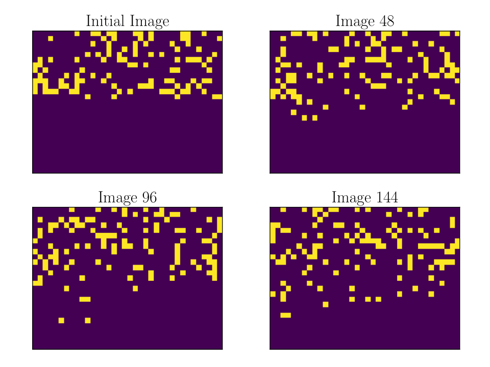
The (discrete) cell model starts with a grid of size $27\times 36$ and $110$ initial cells that are randomly placed in the upper part of the grid. This simulates wound healing, where a part of the tissue was scratched away due to an accident. At each discrete time step, every cell in the grid has a chance of moving to a neighbouring, empty grid position, which is given by the model diffusivity $D$. Similarly, at each discrete time every cell also has a chance to reproduce and spawn a new cell in a neighbouring, empty position, which is dictated by the model proliferation rate $\lambda$. While the model parameters of interest are the diffusivity $D$ and proliferation rate $\lambda$, it is often easier to work with the probability of motility $P_{m}\in[0,1]$ and probability of proliferation $P_{p}\in[0,1]$.¹⁰¹⁰ 10 See how these parameters can be converted in Vo et al. 2015. For a particular combination of $\{P_{m},P_{p}\}$ we can then simulate a time-series of grids where cells move around and reproduce.¹¹¹¹ 11 See Appendix D for a plot showing the spreading of cells under this model. In the context of BED, the discrete design variable is then the time at which to observe this grid and count the total number of cells. In reality, a human would have to physically count the number of cells under a microscope, which is time-consuming, and therefore we want to find the optimal times at which to have the experimenter make an observation. Similar to previous models, we here assume that we have access to a new, independent stochastic process for each sequential iteration.

We shall use 144 time steps as in Vo et al. 2015 and Price et al. 2018b, which means that, including the initial grid, there are 145 grids in every time-series. For the summary statistics used to compute (2.11), we use the Hamming distance between a particular grid and the initial grid, as well as the total number of cells in a particular grid. The one-dimensional design variable is discrete and can take values between 1 and 145, i.e. $d\in\{1,\dots,145\}$, while the summary statistic is two-dimensional. For the model parameters we use prior distributions $p(P_{m})=\mathcal{U}(P_{m};0,1)$ and $p(P_{p})=\mathcal{U}(P_{p};0,0.005)$; we choose the true model parameters to be $P_{m,\text{true}}=0.35$ and $P_{p,\text{true}}=0.001$ as Price et al. 2018b. Because the simulation time for the cell model is significantly more expensive than the previous models we have tested, we only use 300 initial prior samples during the sequential BED algorithm, which we run up to five iterations. We note that, while decreasing the computational resources needed, this may increase the Monte-Carlo error in (3.4) and the error in the LFIRE ratio estimate.

In the top row in Figure 8 we compare the sequential MI utilities for iteration 1 (left) and 5 (right) for the cell model; see Appendix G for a plot showing utilities for all iterations. Shown are the posterior predictive means and variances of the surrogate GP model, the BO evaluations and the respective optima. Because of the discrete domain, a normal GP tends to overfit this data and therefore we have used a one-layer deep GP (Damianou and Lawrence 2013 see) as the surrogate model, which means that the GP hyper-parameters are modelled by GPs as well. For each iteration there seems to be some merit in taking observations at small and large designs but not for medium-large designs, e.g. $d\sim 20-40$. At early designs, not much proliferation will have happened (due to its small prior probability) and so one can more easily measure the effect of motility. Conversely, at large designs one can average out the effect of motility and more easily notice the effect of proliferation, as more time has elapsed. In our case, the information gain about proliferation seems to beat that about motility in iteration $1$, and similarly for iterations $2-4$ (see Appendix G). After having repeatedly made measurements at large designs, at iteration $5$ it becomes more effective to measure at small designs. This is because we have decreased the uncertainty in the proliferation parameter in iterations $1-4$ and then need a measurement at early designs to sufficiently decrease the uncertainty in the motility parameter. Note that we resampled the parameters according to Algorithm 2 before iteration $2$ and $3$, as the effective sample size went below 50%.

Similarly to before, we use KDE and updated belief samples obtained from Algorithm 1 to visualise the approximate posterior densities after every iteration. In the bottom row in Figure 8 we show the posterior densities obtained after iteration $1$ (left) and $5$ (right); see Appendix G for a plot showing posterior distributions after every iteration. After iteration $1$, the updated belief distribution has a wide spread in the $P_{m}$ parameter and is more narrow for the $P_{p}$ parameter. The optimal design at iteration $1$ was at the far end of the design domain at $d^{\ast}_{1}=145$. This is a design that helps to more easily detect the effect of proliferation as opposed to motility, which is reflected in the figure. The same phenomenon occurs in subsequent iterations $2-4$, where the optimal designs are at the far end of the design domain (see Appendix G). This results in posterior distributions that are relatively narrow for $P_{p}$ but wider for $P_{m}$. Taking a measurement at the small design $d_{5}^{\ast}=2$ in iteration $5$, which allows us to more easily detect the effect of motility, reduces the uncertainty in the $P_{m}$ parameter as well, as can be seen in the bottom right plot of Figure 8. The mode of the posterior distribution after iteration $5$ is close to the true parameter value of $P_{m,\text{true}}=0.35$ and $P_{p,\text{true}}=0.001$. The estimated mean of the motility parameter is $\widehat{P}_{m}=0.394$ with a $95\%$ credibility interval of $[0.166,0.642]$, while for the proliferation parameter it is $\widehat{P}_{p}=0.00150$ with a $95\%$ credibility interval of $[0.00055,0.00265]$. Both credibility intervals contain the true parameter values. The credibility intervals were computed using a Gaussian KDE of the marginal posterior samples and the HPDI method.

The cell model demonstrates that we can effectively use MI in sequential BED when the forward simulations are expensive and the design domain is discrete. For this model, an experimenter might intuitively want to take observations at regular intervals but we have seen from the sequential utility functions that the expected information gain may then be sub-optimal. Sequential BED suggests that, when there is a limited budget, it is best to first take observations at high values in the design domain as the effect of proliferation dominates that of motility. Later, however, we should take observations at small designs to reduce the uncertainty in the motility parameter as well.

References

- Agostinelli et al. (2003) Agostinelli, S., Allison, J., Amako, K., Apostolakis, J., M Araujo, H., Arce, P., Asai, M., A Axen, D., Banerjee, S., Barrand, G., Behner, F., Bellagamba, L., Boudreau, J., Broglia, L., Brunengo, A., Chauvie, S., Chuma, J., Chytracek, R., Cooperman, G., and Zschiesche, D. (2003). “GEANT4-a simulation toolkit.” 506: 250.
- Allen (2008) Allen, L. J. S. (2008). Mathematical Epidemiology, chapter An Introduction to Stochastic Epidemic Models, 81–130. Berlin, Heidelberg: Springer Berlin Heidelberg.
- Alsing et al. (2018) Alsing, J., Wandelt, B., and Feeney, S. (2018). “Massive optimal data compression and density estimation for scalable, likelihood-free inference in cosmology.” MNRAS, 477: 2874–2885.
- Arnold et al. (2018) Arnold, B., Gutmann, M., Grad, Y., Sheppard, S., Corander, J., Lipsitch, M., and Hanage, W. (2018). “Weak Epistasis May Drive Adaptation in Recombining Bacteria.” Genetics, 208(3): 1247–1260.
- Bentley (1975) Bentley, J. L. (1975). “Multidimensional Binary Search Trees Used for Associative Searching.” Commun. ACM, 18(9): 509–517.
- Blum and Francois (2010) Blum, M. and Francois, O. (2010). “Non-linear regression models for Approximate Bayesian Computation.” Statistics and Computing, 20(1): 63–73.
- Chen and Gutmann (2019) Chen, Y. and Gutmann, M. U. (2019). “Adaptive Gaussian Copula ABC.” In Chaudhuri, K. and Sugiyama, M. (eds.), Proceedings of the International Conference on Artificial Intelligence and Statistics (AISTATS), volume 89 of Proceedings of Machine Learning Research, 1584–1592.
- Chen (2003) Chen, Z. (2003). “Bayesian Filtering: From Kalman Filters to Particle Filters, and Beyond.” Statistics, 182.
- Cook et al. (2008) Cook, A. R., Gibson, G. J., and Gilligan, C. A. (2008). “Optimal Observation Times in Experimental Epidemic Processes.” Biometrics, 64(3): 860–868.
- Corander et al. (2017) Corander, J., Fraser, C., Gutmann, M., Arnold, B., Hanage, W., Bentley, S., Lipsitch, M., and Croucher, N. (2017). “Frequency-dependent selection in vaccine-associated pneumococcal population dynamics.” Nature Ecology & Evolution, 1: 1950–1960.
- Dale et al. (1994) Dale, P. D., Maini, P. K., and Sherratt, J. A. (1994). “Mathematical modeling of corneal epithelial wound healing.” Mathematical Biosciences, 124(2): 127 – 147.
- Damianou and Lawrence (2013) Damianou, A. and Lawrence, N. (2013). “Deep Gaussian Processes.” In Carvalho, C. M. and Ravikumar, P. (eds.), Proceedings of the Sixteenth International Conference on Artificial Intelligence and Statistics, volume 31 of Proceedings of Machine Learning Research, 207–215. Scottsdale, Arizona, USA: PMLR.
- Dinev and Gutmann (2018) Dinev, T. and Gutmann, M. U. (2018). “Dynamic Likelihood-free Inference via Ratio Estimation (DIRE).” arXiv e-prints, arXiv:1810.09899.
- Doucet and Johansen (2009) Doucet, A. and Johansen, A. (2009). “A Tutorial on Particle Filtering and Smoothing: Fifteen Years Later.” Handbook of Nonlinear Filtering, 12.
- Drovandi et al. (2015) Drovandi, C. C., Pettitt, A. N., and Lee, A. (2015). “Bayesian indirect inference using a parametric auxiliary model.” Statistical Science 2015, 30(1): 72–95.
- Greenberg et al. (2019) Greenberg, D., Nonnenmacher, M., and Macke, J. (2019). “Automatic Posterior Transformation for Likelihood-Free Inference.” In Chaudhuri, K. and Salakhutdinov, R. (eds.), Proceedings of the 36th International Conference on Machine Learning, volume 97 of Proceedings of Machine Learning Research, 2404–2414. Long Beach, California, USA: PMLR.
- Gutmann and Corander (2016) Gutmann, M. and Corander, J. (2016). “Bayesian optimization for likelihood-free inference of simulator-based statistical models.” Journal of Machine Learning Research, 17(125): 1–47.
- Gutmann et al. (2018) Gutmann, M., Dutta, R., Kaski, S., and Corander, J. (2018). “Likelihood-free inference via classification.” Statistics and Computing, 28(2): 411–425.
- Hainy et al. (2016) Hainy, M., Drovandi, C. C., and McGree, J. (2016). “Likelihood-free extensions for Bayesian sequentially designed experiments.” In Kunert, J., Muller, C. H., and Atkinson, A. C. (eds.), 11th International Workshop in Model-Oriented Design and Analysis (mODa 2016), 153–161. Hamminkeln, Germany: Springer.
- Ikonomov and Gutmann (2020) Ikonomov, B. and Gutmann, M. (2020). “Robust Optimisation Monte Carlo.” In Proceedings of the International Conference on Artificial Intelligence and Statistics (AISTATS).
- Järvenpää et al. (2019) Järvenpää, M., Gutmann, M., Vehtari, A., and Marttinen, P. (2019). “Efficient acquisition rules for model-based approximate Bayesian computation.” Bayesian Analysis, 14(2): 595–622.
- Järvenpää et al. (2020) Järvenpää, M., Gutmann, M. U., Vehtari, A., and Marttinen, P. (2020). “Parallel Gaussian process surrogate Bayesian inference with noisy likelihood evaluations.” Bayesian Analysis, in press.
- Kish (1965) Kish, L. (1965). Survey sampling. Chichester : Wiley New York.
- Kleinegesse and Gutmann (2019) Kleinegesse, S. and Gutmann, M. U. (2019). “Efficient Bayesian Experimental Design for Implicit Models.” In Chaudhuri, K. and Sugiyama, M. (eds.), Proceedings of Machine Learning Research, volume 89 of Proceedings of Machine Learning Research, 476–485. PMLR.
- Kullback and Leibler (1951) Kullback, S. and Leibler, R. A. (1951). “On information and sufficiency.” Ann. Math. Statistics, 22: 79–86.
- Lindley (1972) Lindley, D. (1972). Bayesian Statistics. Society for Industrial and Applied Mathematics.
- Lintusaari et al. (2017) Lintusaari, J., Gutmann, M., Dutta, R., Kaski, S., and Corander, J. (2017). “Fundamentals and Recent Developments in Approximate Bayesian Computation.” Systematic Biology, 66(1): e66–e82.
- Lueckmann et al. (2017) Lueckmann, J.-M., Gonçalves, P. J., Bassetto, G., Öcal, K., Nonnenmacher, M., and Macke, J. H. (2017). “Flexible Statistical Inference for Mechanistic Models of Neural Dynamics.” In Proceedings of the 31st International Conference on Neural Information Processing Systems, NIPS’17, 1289–1299. USA: Curran Associates Inc.
- M. Schafer and Freeman (2012) M. Schafer, C. and Freeman, P. (2012). “Likelihood-Free Inference in Cosmology: Potential for the Estimation of Luminosity Functions.” 209: 3–19.
- Marttinen et al. (2015) Marttinen, P., Croucher, N., Gutmann, M., Corander, J., and Hanage, W. (2015). “Recombination produces coherent bacterial species clusters in both core and accessory genomes.” Microbial Genomics, 1(5).
- Meeds and Welling (2015) Meeds, T. and Welling, M. (2015). “Optimization Monte Carlo: Efficient and Embarrassingly Parallel Likelihood-Free Inference.” In Cortes, C., Lawrence, N. D., Lee, D. D., Sugiyama, M., and Garnett, R. (eds.), Advances in Neural Information Processing Systems 28, 2080–2088. Curran Associates, Inc.
- Mockus et al. (1978) Mockus, J., Tiesis, V., and Zilinskas, A. (1978). The application of Bayesian methods for seeking the extremum, volume 2.
- Müller (1999) Müller, P. (1999). “Simulation-Based Optimal Design.” Bayesian Statistics, 6: 459 – 474.
- Numminen et al. (2013) Numminen, E., Cheng, L., Gyllenberg, M., and Corander, J. (2013). “Estimating the Transmission Dynamics of Streptococcus pneumoniae from Strain Prevalence Data.” Biometrics, 69(3): 748–757.
- Overstall and Woods (2017) Overstall, A. M. and Woods, D. C. (2017). “Bayesian Design of Experiments Using Approximate Coordinate Exchange.” Technometrics, 59(4): 458–470.
- Papamakarios and Murray (2016) Papamakarios, G. and Murray, I. (2016). “Fast -free Inference of Simulation Models with Bayesian Conditional Density Estimation.” In Lee, D. D., Sugiyama, M., Luxburg, U. V., Guyon, I., and Garnett, R. (eds.), Advances in Neural Information Processing Systems 29, 1028–1036. Curran Associates, Inc.
- Papamakarios et al. (2019) Papamakarios, G., Sterratt, D., and Murray, I. (2019). “Sequential Neural Likelihood: Fast Likelihood-free Inference with Autoregressive Flows.” In Chaudhuri, K. and Sugiyama, M. (eds.), Proceedings of Machine Learning Research, volume 89 of Proceedings of Machine Learning Research, 837–848. PMLR.
- Price et al. (2018a) Price, D. J., Bean, N. G., Ross, J. V., and Tuke, J. (2018a). “An induced natural selection heuristic for finding optimal Bayesian experimental designs.” Computational Statistics and Data Analysis, 126: 112 – 124.
- Price et al. (2018b) Price, L. F., Drovandi, C. C., Lee, A., and Nott, D. J. (2018b). “Bayesian Synthetic Likelihood.” Journal of Computational and Graphical Statistics, 27(1): 1–11.
- Pritchard et al. (1999) Pritchard, J. K., Seielstad, M. T., Perez-Lezaun, A., and Feldman, M. W. (1999). “Population growth of human Y chromosomes: a study of Y chromosome microsatellites.” Molecular Biology and Evolution, 16(12): 1791–1798.
- Ricker (1954) Ricker, W. E. (1954). “Stock and Recruitment.” Journal of the Fisheries Research Board of Canada, 11(5): 559–623.
- Rubin (1984) Rubin, D. B. (1984). “Bayesianly Justifiable and Relevant Frequency Calculations for the Applied Statistician.” Ann. Statist., 12(4): 1151–1172.
- Ryan et al. (2016) Ryan, E. G., Drovandi, C. C., McGree, J. M., and Pettitt, A. N. (2016). “A Review of Modern Computational Algorithms for Bayesian Optimal Design.” International Statistical Review, 84(1): 128–154.
- Shahriari et al. (2016) Shahriari, B., Swersky, K., Wang, Z., Adams, R. P., and de Freitas, N. (2016). “Taking the Human Out of the Loop: A Review of Bayesian Optimization.” Proceedings of the IEEE, 104(1): 148–175.
- Sisson et al. (2018) Sisson, S., Fan, Y., and Beaumont, M. (2018). Handbook of Approximate Bayesian Computation. Chapman & Hall/CRC Handbooks of Modern Statistical Methods. CRC Press.
- Sjöstrand et al. (2008) Sjöstrand, T., Mrenna, S., and Skands, P. (2008). “A brief introduction to PYTHIA 8.1.” Computer Physics Communications, 178: 852–867.
- Swanson et al. (2003) Swanson, K. R., Bridge, C., Murray, J., and Alvord, E. C. (2003). “Virtual and real brain tumors: using mathematical modeling to quantify glioma growth and invasion.” Journal of the Neurological Sciences, 216(1): 1 – 10.
- Thomas et al. (2016) Thomas, O., Dutta, R., Corander, J., Kaski, S., and Gutmann, M. U. (2016). “Likelihood-free inference by ratio estimation.” ArXiv e-prints: 1611.10242.
- Vo et al. (2015) Vo, B. N., Drovandi, C. C., Pettitt, A. N., and Simpson, M. J. (2015). “Quantifying uncertainty in parameter estimates for stochastic models of collective cell spreading using approximate Bayesian computation.” Mathematical Biosciences, 263: 133 – 142.
- Wilkinson (2014) Wilkinson, R. (2014). “Accelerating ABC methods using Gaussian processes.” In Kaski, S. and Corander, J. (eds.), Proceedings of the Seventeenth International Conference on Artificial Intelligence and Statistics, volume 33 of Proceedings of Machine Learning Research, 1015–1023.
- Wood (2010) Wood, S. N. (2010). “Statistical inference for noisy nonlinear ecological dynamic systems.” Nature, 466: 1102.