Chiral Luttinger liquids in graphene tuned by irradiation

One of the main reasons for the intense interest in bilayer graphene in recent years has been the fact that it has a tunable band gapMcCann2006; Castro2007; Oostinga2008; Zhang2009; McCann2012 modulated by an applied gate voltage, unlike the single layer caseCastroNeto2009 which typically require staggered fields to open up a gap. More recently, it has been realised that it is possible to confine electrons in gated bilayer structures by applying inhomogeneous electric fieldsMartin2008 in such a way that one dimensional states can be formed at the domain walls separating the two different insulating regions with different gate voltages. These states are similar to the zero modes that form at domain walls in polyacetylineHeeger1988, superconducting vorticesSemenoff2008 or other solitons in field theoriesJackiw1976. They are free to move in the direction perpendicular to their confinement and are hence nanowires which can be tuned by the gate voltages. The effect of electron-electron interactions on such wires have also been studiedKilli2010 and it has been demonstrated that these one-dimensional nanowires behave like strongly interacting Luttinger liquids. Thus bilayer graphene has been shown to be a useful substrate to create and manipulate strongly interacting one-dimensional quantum wires.

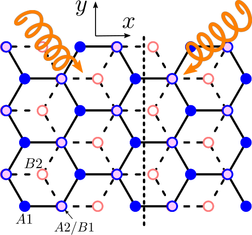
Floquet engineeringlindner2011; dora2012; rudner2013; goldman2014; farrell2015; titum2016; klinovaja2016; seradjeh2018 or the generation of new Hamiltonians that are not present in static systems but emerge in driven systems, have recently become a very important field of study. In the case of graphene, it has been realised that the possibility of tuning the band gap by shining light greatly increases the potential of applications and there has been considerable workoka2009; kitagawa2011; kundu2014; usaj2014; fkundu2016; mikami2016; mohan2016; mukherjee2017; mishra2018; mishra2015 on new topological phases obtained by shining light on graphene, as well as bilayer graphenemorell2012; dallago2017; iorsh2017; mohan2018. Recent experimental observation of anomalous Hall effect in irradiated graphene confirms the Floquet bands and their non-trivial Berry curvature graexp. Since shining light changes the electric field acting on the electrons in graphene or bilayer graphene, a natural question to ask is whether it would be possible to create confinement of electrons using inhomogeneous light instead of an inhomogeneous electric field using gates. As we shall see in this paper, the answer to this question can be answered positively. Moreover, unlike externally applied voltages, shining light breaks the time reversal invariance of the system, and so we find that the edge states that are created by confinement by light are chiral in nature.

Our main focus in this paper will be on the chiral edge modes that emerge at the interface where there is a change in the polarization or phase of the circularly polarized light (CPL) applied perpendicular to the plane of either a single-layer graphene (SLG) or an $A$-$B$ stacked bi-layer graphene (BLG). We shall show that the steady-state edge modes near each of the valleys turn out to be chiral (either both left-handed or both right-handed), since they result from the breaking of time reversal by light. For high frequency driving, these modes are time-independent and in the presence of Coulomb interaction, the interactions between the modes are also essentially time-independent. We shall then show that Coulomb interaction between these chiral modes leads to their mixing, which can then be rediagonalised using the standard techniques of bosonisation and Luttinger liquids. We can then obtain the power law behaviour of the charge density and spin density correlation functions and show that the exponents, which should be sensitive to scanning tunneling measurements, can be tuned by changing the amplitude of the impinging radiation. Although we model our system based on single or bi-layer graphene, the qualitative aspects of the resulting chiral Luttinger liquid physics we expect to be model independent and similar treatment can be made for other topological edge-modes of driven symmetry-broken phases.

We consider the model of bi-layer graphene below and analyze the resulting effective static Hamiltonian in the high-frequency limit. The results of a single-layer of graphene can be recovered in the absence of inter-layer hoppings. The Hamiltonian, for the electrons of each spin, on bi-layer graphene contains the Hamiltonian of each of the single-layers, $H_{\text{SLG}}$, and a coupling Hamiltonian between the layers, $H_{\text{inter}}$:

	$\displaystyle H_{\text{SLG}}$	$\displaystyle=-t\sum_{\langle ij\rangle,l}a^{\dagger}_{l,i}b_{l,j}+\text{h.c.}$		(1)
	$\displaystyle H_{\text{inter}}$	$\displaystyle=t_{p}\sum_{i\in A,j\in B}a^{\dagger}_{2,i}b_{1,j}+\text{h.c.},$		(2)

where $l=1,2$ denotes the layer index, and $a^{\dagger}$ and $b^{\dagger}$ are, respectively, the creation operators for the $A$ and $B$-sublattices of each of the layers. $t$ and $t_{p}$ are, respectively, the intra and inter-layer hopping amplitudes and we take the estimation $t_{p}=0.1t$ with $t=2.7$eV. For each single-layer, if not coupled to a second layer, the electrons follow an effective relativistic dispersion near the two distinct Dirac nodes $K,K^{\prime}$ with the Fermi velocity $\nu$ given by $\hbar\nu=\frac{3}{2}ta_{0}$, where $a_{0}$ is the lattice constant. For the rest of the paper we set $\hbar=a_{0}=1$, which serves as our unit of energy and length, respectively. We consider Bernal stacking of the two layers, where the inter-layer hopping amplitudes are only between the $B$-sublattice of the top layer and the $A$-sublattice of the bottom layer, as shown in the Fig. 1.

The low energy Hamiltonian, at a single Dirac node is given by McCann2006; Martin2008

$\displaystyle H=\begin{pmatrix}0&\nu\pi^{\dagger}&0&0\\ \nu\pi&0&t_{p}&0\\ 0&t_{p}&0&\nu\pi^{\dagger}\\ 0&0&\nu\pi&0\end{pmatrix},$

(3)

written in the basis of the wave-functions $\Psi=(\psi_{A1},\psi_{B1},\psi_{A2},\psi_{B2})$. The canonical momenta are defined as $\pi=p_{x}+ip_{y},\pi^{\dagger}=p_{x}-ip_{y}$, in terms of the quasimomentum operators $p_{x}$ and $p_{y}$.

We now apply high frequency circularly polarized light (CPL) perpendicular to the plane of the layers. The vector potential of the radiation is of the form

$\displaystyle\mathbf{A}(t)=(A_{x}\cos(\omega t),A_{y}\sin(\omega t+\theta),0),$

(4)

where $\omega$ is the frequency of the light and $\theta$ is its polarization angle. To work legitimately in the low energy sector around a single Dirac node, post the application of radiation, we need to assume that the amplitudes $A_{x}$ and $A_{y}$ are weak enough to allow a linear dispersion approximation to hold. The Hamiltonian for the bilayer in the presence of such a driving force is given by

$$\mathcal{H}(t)=\begin{pmatrix}0&\nu\tilde{\pi}^{\dagger}(t)&0&0\\ \nu\tilde{\pi}(t)&0&t_{p}&0\\ 0&t_{p}&0&\nu\tilde{\pi}^{\dagger}(t)\\ 0&0&\nu\tilde{\pi}(t)&0\end{pmatrix}$$

(5)

where,

$\displaystyle\tilde{\pi}(t)$

$\displaystyle=\left(p_{x}-eA_{x}\cos(\omega t)\right)+i\left(p_{y}-eA_{y}\sin(\omega t+\theta)\right)$

denotes the canonical momentum with the gauge field $\mathbf{A}(t)$ being included in $\mathcal{H}$ in a minimally coupled fashion, with $e$ being the electronic charge and setting the speed of light $c=1$. Since we take the frequency of the light to be very high, $i.e.$, much larger than all other scales (such as intra-layer or inter-layer hoppings) in the problem, it is possible to compute an effective time-independent Hamiltonian for the system. There are several high frequency approximationsmikami2016; Feldman1984; Mananga2011; Casas2001; Kuwahara2016; Eckardt2015; Bukov2015 that one can use to obtain the static Hamiltonian, all of which agree to first order in the inverse frequency $1/\omega$. Using such an approximation, one obtains the effective static Hamiltonian, given by

$\displaystyle H_{\rm eff}\approx\mathcal{H}_{0}+\frac{1}{\omega}\displaystyle\sum_{n=1}^{\infty}\frac{[\mathcal{H}_{n},\mathcal{H}_{-n}]}{n}+\mathcal{O}(\omega^{-2})~.$

(6)

Here $\mathcal{H}_{n}$ denote the Fourier coefficients of the periodic time-dependent Hamiltonian ($\mathcal{H}(t)$ in Eq.(5) in our case), and $[,]$ denotes a commutator bracket. Rewriting the Hamiltonian $\mathcal{H}(t)$ in Eq.(5) as

$$\mathcal{H}(t)=\mathcal{H}_{0}+\mathcal{H}_{1}e^{i\omega t}+\mathcal{H}_{-1}e^{-i\omega t}$$

we obtain

$$\mathcal{H}_{0}=\begin{pmatrix}0&\nu\pi^{\dagger}&0&0\\ \nu\pi&0&t_{p}&0\\ 0&t_{p}&0&\nu\pi^{\dagger}\\ 0&0&\nu\pi&0\end{pmatrix}$$

and the Fourier coefficients $\mathcal{H}_{n=\pm 1}$ as

$$\mathcal{H}_{\pm 1}=\begin{pmatrix}0&-\frac{\lambda}{2}(A_{x}\mp A_{y}e^{\pm i\theta})&0&0\\ -\frac{\lambda}{2}(A_{x}\pm A_{y}e^{\pm i\theta})&0&0&0\\ 0&0&0&-\frac{\lambda}{2}(A_{x}\mp A_{y}e^{\pm i\theta})\\ 0&0&-\frac{\lambda}{2}(A_{x}\pm A_{y}e^{\pm i\theta})&0\end{pmatrix}$$

where, $\lambda=\nu e$. The effective, time-independent Hamiltonian for the BLG system driven by high-frequency CPL is thus obtained as

$$H_{\rm eff}=\begin{pmatrix}-\frac{\lambda^{2}\gamma}{4\omega}\cos\theta&\nu\pi^{\dagger}&0&0\\ \nu\pi&\frac{\lambda^{2}\gamma}{4\omega}\cos\theta&t_{p}&0\\ 0&t_{p}&-\frac{\lambda^{2}\gamma}{4\omega}\cos\theta&\nu\pi^{\dagger}\\ 0&0&\nu\pi&\frac{\lambda^{2}\gamma}{4\omega}\cos\theta\end{pmatrix}$$

(7)

where $\gamma=4A_{x}A_{y}$. Hence, the effect of the CPL, in the high frequency limit, is essentially to introduce an on-site modulation on the sublattice sites of the two layers, amounting to a sublattice staggering potential at the $A$ and $B$ sites of both layers. Thus, we would expect that shining light gives rise to an effective Haldane gap at both the valleys.

In the above effective Hamiltonian, if we set $t_{p}=0$, we recover the effective Hamiltonian for each of the single layers of the graphene as

$\displaystyle H^{\rm SLG}_{\rm eff}=\begin{pmatrix}-\frac{\lambda^{2}\gamma}{4\omega}\cos\theta&\nu\pi^{\dagger}\\ \nu\pi&\frac{\lambda^{2}\gamma}{4\omega}\cos\theta,\end{pmatrix}$

(8)

which has the form of a two-dimensional Dirac equation with the mass term given by $m=\frac{\lambda^{2}\gamma}{4\omega}\cos\theta$. This immediately implies that the sign of the mass term, and thus the Chern number can be modified by changing the sign of $\cos\theta$, near each of the Dirac points. If we have opposite polarization of the irradiation for $x>0$ and $x<0$, then this gives rise to two resulting topological edge-modes at $x=0$, of the same chirality, one each near momenta $K$ and $K^{\prime}$.

For the case of bi-layer graphene, our next step is to compute the effective low energy two band model which describes the physics from the four-band Hamiltonian Eq. (7) using a prescriptionManes2007 similar to that which has been used for gated bilayer grapheneMartin2008. To do that, we first rewrite the $H_{\rm eff}$ in a modified site basis $(A1,B2,B1,A2)$ where the effective Hamiltonian takes the form,

	$\displaystyle H_{\rm eff}=$	$\displaystyle\begin{pmatrix}-\frac{\lambda^{2}\gamma}{4\omega}\cos\theta&0&\nu\pi^{\dagger}&0\\ 0&\frac{\lambda^{2}\gamma}{4\omega}\cos\theta&0&\nu\pi\\ \nu\pi&0&\frac{\lambda^{2}\gamma}{4\omega}\cos\theta&t_{p}\\ 0&\nu\pi^{\dagger}&t_{p}&-\frac{\lambda^{2}\gamma}{4\omega}\cos\theta\end{pmatrix}$
	$\displaystyle\equiv$	$\displaystyle\begin{pmatrix}H_{11}&H_{12}\\ H_{21}&H_{22}\end{pmatrix}$		(9)

where $H_{ij}$ denote the appropriate $2\times 2$ blocks. The eigenvalues $\epsilon$ of $H_{\rm eff}$ can then be shown to follow the identity

	$\displaystyle{\rm det}(H_{\rm eff}-\epsilon)$	$\displaystyle={\rm det}(H_{11}-H_{12}(H_{22}-\epsilon)^{-1}H_{21}-\epsilon)$
		$\displaystyle\quad\quad\times{\rm det}(H_{22}-\epsilon).$		(10)

In the low energy regime where $\epsilon\ll t_{p}$ and where $\frac{\lambda^{2}\gamma}{4\omega}\ll t_{p}$, since $H_{22}-\epsilon\simeq H_{22}$, we can project the 4-band Hamiltonian onto the two low energy bands, given by the Hamiltonian

$$\begin{split}H^{L}_{\rm eff}&=H_{11}-H_{12}H^{-1}_{22}H_{21}\\ &=\begin{pmatrix}-\frac{\lambda^{2}\gamma}{4\omega}\cos\theta\left(1+\frac{\nu^{2}p^{2}}{t^{2}_{p}}\right)&-\frac{\nu^{2}\pi^{{\dagger}^{2}}}{t_{p}}\\ -\frac{\nu^{2}\pi^{2}}{t_{p}}&\frac{\lambda^{2}\gamma}{4\omega}\cos\theta\left(1+\frac{\nu^{2}p^{2}}{t^{2}_{p}}\right)\end{pmatrix}\end{split}$$

(11)

where $p=(\pi\pi^{\dagger})^{\frac{1}{2}}=\sqrt{p^{2}_{x}+p^{2}_{y}}$. Under the approximation where we drop the second term in the diagonal part of the Hamiltonian, this Hamiltonian becomes very similar to the Hamiltonian derived for gated bi-layer grapheneMartin2008. In this approximation, the potential terms on the diagonal and the momentum dependent terms on the off-diagonal parts of the Hamiltonian are decoupled. Any position dependence in this Hamiltonian can now be introduced in the system consistently by simply promoting $p_{x}$ and $p_{y}$ to their corresponding differential operator representations. This allows the eigenvalue problem to be duplicated by a quasi-classical Hamiltonian of the kind derived in Ref.(Martin2008), written as

$$\tilde{H}^{L}_{\rm eff}=-\phi(x)\sigma_{z}-(p^{2}_{x}-p^{2}_{y})\sigma_{x}-2p_{x}p_{y}\sigma_{y}$$

(12)

where $\phi(x)=t^{2}_{p}a_{0}^{2}/2\nu^{2}\times(\lambda^{2}\gamma\cos\theta/4\omega)$ in our case and momenta are measured in units of inverse lattice constant (i.e., $1/a_{0}$). For the case of a bilayer strip which is finite in the $x$ direction and translationally invariant in $y$, $p_{y}$ is a good quantum number whereas $p_{x}$ is an operator. Hence, we need to solve the pair of coupled differential equations, obtained from the eigenvalue problem for the Hamiltonian in eq.(12), for the potential profile contained in $\phi(x)$. When $\phi(x)$ has a step profile, changing sign across a boundary, topological zero-energy modes are localized at the kink or the domain wall. In our case, we introduce a position dependence in the polarization angle of the irradiation and study the domain wall obtained when we have light of two different polarizations for $x<0$ and $x>0$.

In fact, the Chern number associated with the ground-state of Eq. (12) is given by sgn($\phi$), which is easily seen as following. We rewrite the effective Hamiltonian, Eq. (12), as

$\displaystyle\tilde{H}_{\text{eff}}^{L}$

$\displaystyle\equiv\begin{bmatrix}-\phi&k^{2}\text{e}^{2i\theta}\\ k^{2}\text{e}^{-2i\theta}&\phi\\ \end{bmatrix},$

(13)

with $k=\sqrt{k^{2}_{y}+k^{2}_{x}}$ and $\theta=\tan^{-1}(\frac{k_{x}}{k_{y}})$. Diagonalization gives the the wave-functions

$\displaystyle\Psi_{\pm}=\begin{bmatrix}\text{e}^{i\theta}\frac{k^{2}}{\sqrt{k^{4}+(\phi\pm\sqrt{\phi^{2}+k^{4}})^{2}}}\\ \text{e}^{-i\theta}\frac{\phi\pm\sqrt{\phi^{2}+k^{4}}}{\sqrt{k^{4}+(\phi\pm\sqrt{\phi^{2}+k^{4}})^{2}}}\\ \end{bmatrix}$

(14)

with energies $\epsilon_{\pm}=\pm\sqrt{\phi^{2}+k^{4}}$. For the lower energy band, the Chern number is then readily given by

$\displaystyle\frac{i}{2\pi}\int d^{2}k[\langle\partial_{k_{x}}\Psi_{-}|\partial_{k_{y}}\Psi_{-}\rangle-\langle\partial_{k_{y}}\Psi_{-}|\partial_{k_{x}}\Psi_{-}\rangle]=\text{sgn}(\phi).$

(15)

This implies a change of Chern number of $\Delta C$ = 2 across the boundary of regions with different signs of $\phi$, i.e, in the case where the two sides are driven with different polarizations $\phi=+\pi$ and $\phi=-\pi$.

All of this is at a single Dirac point. At the other Dirac point, the operators $\pi$ and $\pi^{\dagger}$ are interchanged. It is easy to check that this only leads to a change in sign in the effective potential term $\phi(x)$ in Eq. (12). So essentially, the operators at the $K$ and $K^{\prime}$ points are related by the symmetry $\phi(x)\rightarrow-\phi(x),~p_{y}\rightarrow-p_{y}$. This, in turn, comes from the fact that the effect of radiation essentially acts like a time-reversal symmetry breaking staggered potential and so, unlike in the gated bi-layer graphene system, the edge states at both the $K$ and the $K^{\prime}$ valleys have the same chirality (decided by the chirality of the circular polarization of the impinging light).

In the previous section, we discussed how the polarized irradiation induces topological gaps at the $K,K^{\prime}$ Dirac points. If the regions irradiated by opposite polarizations are separate, as shown in Fig. 1, one expects edge modes at the interface. If the two sides are irradiated by right and left circularly polarized light (i.e, $\theta=0,\pi$ on the two sides with $A_{x}=A_{y}=A_{0}$), the net change of Chern number across the interface is two (four) for single-layer (bi-layer) graphene and accordingly one expects two (four) chiral modes to run along the interface. We study the edge-modes through a tight-binding simulation, by incorporating the vector-potential Eq. (4) in the Hamiltonian Eq. (1) by Peierls substitution, neglecting the phase difference in $\vec{A}(t)$ between the two layers, which is justified as $l_{\text{int}}\omega/c\ll 1$, where $c$ is the velocity of light and $l_{\text{int}}$ is the inter-layer distance. The steady states of the time-periodic Hamiltonian, $H(t)$, after the Peierls substitution can be found using the Floquet theorem, which states that the eigen-states will be of the form

$\displaystyle\psi_{\alpha}(t)=e^{-i\epsilon_{\alpha}t}u_{\alpha}(t),$

(16)

where $\epsilon_{\alpha}$s are the ‘quasienergies’ and $u_{\alpha}(t)$ are periodic functions, called the Floquet-states, both of which can be found from the eigen-system problem

$\displaystyle(i\partial_{t}-H(t))u_{\alpha}(t)=\epsilon_{\alpha}u_{\alpha}(t).$

(17)

For a high-frequency drive, the quasi-energy spectrum of a nano-ribbon, as depicted in Fig. 1, is shown in Fig. 2, highlighting the edge-modes. The edge-modes appear at each $K/K^{\prime}$ points with a slightly different Fermi velocity $v_{1}$ and $v_{2}$. (The Appendix has a discussion of how higher orders in the high frequency expansion lead to the fact that $v_{1}\neq v_{2}$).

Before we proceed to analyze the properties of the topological edge-modes under Coulomb interactions, which we introduce perturbatively, a justification of the use of the non-interacting Floquet analysis is due. A number of recent worksheating1; heating2; heating3; heating4 argue that, for a rapidly driven closed interacting system, the heating time ($\tau_{h}$) scale is exponentially large in the driving frequency and in the intermediate time the system’s dynamics is governed by an effective Hamiltonian, which one may obtain from a high-frequency approximation, such as the van Vleck expansion used in our system. If our system is weakly connected to an environment, giving rise to a relaxation time scale $\tau_{l}$, then as long as $\tau_{l}\ll\tau_{h}$, one expects the system to not be heated. Further, with a high-frequency drive, even when there is a gap-opening due to the breaking of a symmetry, such as in our case, one expects no population inversion heating5; heating6. This allows us to consider the occupations to have the standard Fermi-Dirac distribution. We further consider that the bulk system, which has Dirac dispersion near the Fermi-energy, is essentially non-interacting and that the Coulomb interaction is only important in the edge-modes. This assumption, strictly speaking, needs to be further justified, and can be argued as follows. First, since the edge-modes are topological, they are expected to be robust against weak interactions in the bulk. Second, since the edge modes are one-dimensional, the effect of Coulomb interaction among them can not be neglected.

Assuming that the preceding approximations hold, we further proceed to make an another argument to justify the application of Luttinger liquid theory - namely, we argue that the interaction among the edge-modes are also effectively time-independent. In the presence of perturbative interactions, the effective interaction elements among modes with similar quasi-energies can be written as

$\displaystyle\langle\psi_{\alpha}(t)|\hat{V}_{\text{int}}|\psi_{\alpha^{\prime}}(t)\rangle=\langle u_{\alpha}(t)|\hat{V}_{\text{int}}|u_{\alpha^{\prime}}(t)\rangle,$

(18)

where we used the fact that $\epsilon_{\alpha}=\epsilon_{\alpha^{\prime}}$. Expanding in Fourier components, $|u_{\alpha}(t)\rangle=\sum_{n}e^{-in\omega t}|u_{\alpha}^{(n)}\rangle$, the right hand side of the above equation can be written as

$\displaystyle=\sum_{n,m}e^{i(n-m)\omega t}\langle u^{(n)}_{\alpha}|\hat{V}_{\text{int}}|u_{\alpha^{\prime}}^{(m)}\rangle.$

(19)

We show in Fig. 3 that for the edge-modes, $|u_{\alpha}^{(0)}\rangle$ is dominant, and other Fourier components can be neglected (i.e, the time-dependence of $\psi_{\alpha}(t)$ is governed by only the dynamical phase factor). This essentially results from the fact that the gap opening (and thus the resulting edge-modes) at the $K,K^{\prime}$ points takes place even for an infinitesimal driving amplitude without any relevant change of occupation number heating5; heating6. This allows us to simplify the interaction matrix elements among the edge modes to be effectively time-independent.

These edge-states are also expected from the effective static Hamiltonian obtained by the high-frequency approximation in the last section. Since there exists a difference in Chern number between regions of different sign of $\phi$ (i.e, of opposite polarization), it is clear that the regions are topological and that the boundary must have edge states. The simplest possibility ( in the absence of further counter-propagating states) is to have as many chiral edge states as dictated by the change in Chern number. As the effective static Hamiltonian can only predict dynamics in stroboscopic times Eckardt2015, the states may still have significant transverse dynamics. We check this in Fig. 3, where, we examine the transverse dispersion of a wave-packet, initially introduced at the domain-wall of the two topologically distinct regions, when driven by the time-periodic Hamiltonian. The results show that, for a few hundred cycles, the wave-packet can be considered to be confined at the interface of the two regions, although for BLG (unlike for SLG), the wave packet starts spreading for about a 1000 cycles. In contrast, if the dynamics had been strictly driven by a time-independent effective Hamiltonian, as was derived in the last section, we would have found that the wave-packet would have remained confined to the interface for a much longer time. This hints at a non-vanishing transverse velocity and a limit to the time-scale for the validity of the effective one-dimensional nature of the low-energy excitations.

It should also be noted that if the original wave-packet had been prepared in the state of $|u_{\alpha}(t)\rangle$ (or, equivalently, $\approx|u_{\alpha}^{(0)}\rangle$), the wave-packet would have been confined to the boundary for an infinite time, as the Floquet-states are eigenstates of the Hamiltonian. This, however, would require careful initial state-preparation, which may not be an easy task.

As argued in the previous section, the steady-state edge-modes in this system are essentially time-independent, allowing us to consider an effective time-independent interaction Hamiltonian, which is crucial for our use of Luttinger liquid theory bukov2012. Keeping this in mind, we write the interaction among the (effectively time-independent) edge-states of the time-periodic Hamiltonian as

$\displaystyle H_{int}=\frac{1}{2}\int d\vec{r}d\vec{r^{\prime}}\hat{\rho}(\vec{r})V(\vec{r}-\vec{r^{\prime}})\hat{\rho}(\vec{r^{\prime}})~.$

(20)

Here we assume that $\hat{\rho}(r)$ has a trivial time-dependence, which we justify as follows. We write the field operator of the driven system as $\Psi^{\dagger}(\vec{r},t)=\sum_{\alpha}\langle\vec{r}|u_{\alpha}(t)\rangle a_{\alpha}^{\dagger}=\sum_{\alpha,n}e^{i(\epsilon_{\alpha}+n\omega)t}\langle\vec{r}|u^{(n)}_{\alpha}\rangle a_{\alpha}^{\dagger}$, where $|u_{\alpha}(t)\rangle=\sum_{n}e^{-in\omega t}|u^{(n)}_{\alpha}\rangle$ are the Floquet states as defined earlier as well. Then,

	$\displaystyle\hat{\rho}(\vec{r},t)$	$\displaystyle=\Psi^{\dagger}(\vec{r},t)\Psi(\vec{r},t)=\sum_{\alpha,\beta}\sum_{n,m}e^{i(\epsilon_{\alpha}-\epsilon_{\beta})t}\left[e^{i(n-m)\omega t}\langle u^{(m)}_{\beta}|\vec{r}\rangle\langle\vec{r}|u^{(n)}_{\alpha}\rangle\right]a^{\dagger}_{\alpha}a_{\beta}$
		$\displaystyle=\sum_{\alpha,\beta}e^{i(\epsilon_{\alpha}-\epsilon_{\beta})t}\left[\sum_{n}\langle u^{(n)}_{\beta}|\vec{r}\rangle\langle\vec{r}|u^{(n)}_{\alpha}\rangle\right]a^{\dagger}_{\alpha}a_{\beta}+\sum_{\alpha,\beta}e^{i(\epsilon_{\alpha}-\epsilon_{\beta})t}\left[\sum_{n,m\neq n}e^{i(n-m)\omega t}\langle u^{(m)}_{\beta}|\vec{r}\rangle\langle\vec{r}|u^{(n)}_{\alpha}\rangle\right]a^{\dagger}_{\alpha}a_{\beta}.$

So, if $\langle\vec{r}|u^{(0)}\rangle\gg\langle\vec{r}|u^{(n\neq 0)}\rangle$ is satisfied, then generally the non-trivial time dependence of the above equation (second part) can be dropped. As mentioned before, we have verifed this in Figs. 3(a) and 3(b). Further, we also studied wave-packet dynamics of a Gaussian wave-packet in Figs. 3(c) and 3(d) where we obtained a time-scale below which any transverse motion due to the dynamics of the edge-states can be neglected and a Luttinger liquid formalism based on the time-independent density operator can be justified.

Within the effective time-independent description, at low-energy, we have one chiral mode at each of the Dirac points $K,K^{\prime}$ for each spin ($\sigma$) for the SLG and we have two chiral modes at each of the Dirac points $K,K^{\prime}$ for each spin ($\sigma$) for the BLG. We index these modes by $\alpha=K,K^{\prime}$ for the SLG and $\alpha=1_{K},2_{K},1_{K^{\prime}},2_{K^{\prime}}$ for the BLG. Assuming translation invariance along the $y$ direction, we can further write the field operator for each mode, taking into account only the modes near the Fermi energy, with $\vec{R}=(x,y)$ as

$\displaystyle\hat{\Psi}_{\sigma}(\vec{R})=\hat{\Psi}_{\sigma}(x,y)=\sum_{\alpha}\phi_{\alpha}(x)e^{ik^{\alpha}_{F}y}\hat{\xi}_{\alpha\sigma}(y)~,$

(21)

where $\hat{\xi}_{\alpha\sigma}(y)$ is a slowly varying function along $y$. There are a total of eight modes (two modes near each of the Dirac points $K,K^{\prime}$, which are degenerate in spins). The interaction Hamiltonian can then be expressed as

	$\displaystyle\tilde{H}_{int}=$	$\displaystyle\frac{1}{2L_{y}}\sum_{\sigma\sigma^{\prime}yy^{\prime}}\int dydy^{\prime}~\hat{\Psi}^{\dagger}_{\sigma}(\vec{R})\hat{\Psi}^{\dagger}_{\sigma^{\prime}}(\vec{R^{\prime}})V(|\vec{R}-\vec{R^{\prime}}|)$
		$\displaystyle~~~~~~~~~~~~~~~~~~~~~~~~~~~~~~~~~~\times\hat{\Psi}_{\sigma^{\prime}}(\vec{R^{\prime}})\hat{\Psi}_{\sigma}(\vec{R})~,$
		$\displaystyle\equiv\frac{1}{2}\sum_{\sigma\sigma^{\prime}yy^{\prime}\{\alpha\}}\int dydy^{\prime}\ \ h,$		(22)

where the integrand can be written as

	$\displaystyle h$	$\displaystyle=\frac{e^{iy\Delta k-i\bar{y}(k^{\gamma}_{F}-k^{\beta}_{F})}}{\sqrt{{\bar{y}}^{2}+(x-x^{\prime})^{2}}}\phi^{*}_{\alpha}(x)\phi^{*}_{\beta}(x^{\prime})\phi_{\gamma}(x^{\prime})\phi_{\delta}(x)$
		$\displaystyle\quad\quad~~~~~~~\hat{\xi}_{\alpha\sigma}^{\dagger}(y)\hat{\xi}_{\beta\sigma^{\prime}}^{\dagger}(y-\bar{y})\hat{\xi}_{\gamma\sigma^{\prime}}(y-\bar{y})\hat{\xi}_{\delta\sigma}(y),$		(23)

where $\bar{y}=y-y^{\prime}$ and considering the functions $\hat{\xi}$ to be slowly varying, momentum conservation requires $\Delta k=0$. Note that we have assumed that the potential $V(|{\bf R}-{\bf R^{\prime}}|)$ is of the form $e^{2}/\sqrt{{{\bar{y}}^{2}+(x-x^{\prime})^{2}}}$.

Broadly speaking, the possible scattering processes can be divided into two classes, shown as class I and class II in Fig. 4. Computing the bare scattering amplitudes of all the processes, we find that density-density type interactions (class I) are the dominant ones by several orders of magnitude and hence, we keep only such processes. Furthermore, since all scatterings in class I take place in the same mode, we may take $k_{F}^{\gamma}=k_{F}^{\beta}$. In this case, the form of $h$ can be written as

	$\displaystyle h$	$\displaystyle=\frac{1}{\sqrt{\bar{y}^{2}+(x-x^{\prime})^{2}}}\phi^{*}_{\alpha}(x)\phi^{*}_{\beta}(x^{\prime})\phi_{\beta}(x^{\prime})\phi_{\alpha}(x)$
		$\displaystyle\quad\quad~~~~~~~\hat{\xi}_{\alpha\sigma}^{\dagger}(y)\hat{\xi}_{\beta\sigma^{\prime}}^{\dagger}(y-\bar{y})\hat{\xi}_{\beta\sigma^{\prime}}(y-\bar{y})\hat{\xi}_{\alpha\sigma}(y).$		(24)

We may now write the one-dimensional form of the interaction Hamiltonian in terms of the standard two-body scattering amplitudes $V_{\alpha\alpha^{\prime}\alpha^{\prime}\alpha}$ defined below as

	$\displaystyle\tilde{H}_{int}$	$\displaystyle\approx\frac{\alpha_{g}}{2}\int dy\sum_{\alpha\alpha^{\prime}}V_{\alpha\alpha^{\prime}\alpha^{\prime}\alpha}$
		$\displaystyle~~~~~~~~\times\sum_{\sigma\sigma^{\prime}}\hat{\xi}_{\alpha\sigma}^{\dagger}(y)\hat{\xi}_{\alpha^{\prime}\sigma^{\prime}}^{\dagger}(y)\hat{\xi}_{\alpha^{\prime}\sigma^{\prime}}(y)\hat{\xi}_{\alpha\sigma}(y),$		(25)

where the scattering amplitudes are given by

		$\displaystyle V_{\alpha\alpha^{\prime}\alpha^{\prime}\alpha}=\sum_{xx^{\prime}\bar{x}\{\alpha\}}\frac{1}{\sqrt{\bar{y}^{2}+(x-x^{\prime})^{2}}}$
		$\displaystyle~~~~~~~~~~~~~~~~~~~~\times\phi^{*}_{\alpha}(x)\phi^{*}_{\alpha^{\prime}}(x^{\prime})\phi_{\alpha^{\prime}}(x^{\prime})\phi_{\alpha}(x).$		(26)

An effective fine-structure constant $\alpha_{g}\approx 2$ for single-layer graphene is used, and we write all velocities in terms of the velocity of electrons in graphene. For bosonization we adopt the following notations: $\hat{\xi}_{\alpha\sigma}(y)\sim e^{-i2\sqrt{\pi}\Phi_{\alpha\sigma}(y)};~\rho_{\alpha\sigma}(y)=\hat{\xi}^{\dagger}_{\alpha\sigma}(y)\hat{\xi}_{\alpha\sigma}(y)=-\frac{1}{\sqrt{\pi}}\nabla\Phi_{\alpha\sigma}.$ Here $\Phi_{\alpha\sigma}(y)$ is the bosonic field operator. Note that we have not included Klein factors, as they can be set to unity in the density and they do not affect the correlation functions that we compute in this paper. In this notation, the density-density interaction becomes

$\displaystyle\rho_{\alpha\sigma}\rho_{\alpha^{\prime}\sigma^{\prime}}=$

$\displaystyle\frac{1}{\pi}\nabla\Phi_{\alpha\sigma}(y)\nabla\Phi_{\alpha^{\prime}\sigma^{\prime}}(y).$

(27)

Writing $\tilde{H}=\tilde{H}_{o}+\tilde{H}_{int}=\int dx[H_{0}+H_{int}]=\int dxH$, the Hamiltonian can be written in the bosonic language as

	$\displaystyle H=H_{0}+H_{int}=$	$\displaystyle\sum_{\alpha\sigma}v^{\alpha}_{F}(\nabla\Phi_{\alpha\sigma})^{2}$
	$\displaystyle+$	$\displaystyle\frac{1}{2\pi}\sum_{\alpha\alpha^{\prime}}V_{\alpha\alpha^{\prime}\alpha^{\prime}\alpha}\sum_{\sigma\sigma^{\prime}}\nabla\Phi_{\alpha\sigma}\nabla\Phi_{\alpha^{\prime}\sigma^{\prime}}.$		(28)

where the sums over the $\alpha$ and $\sigma$ indices include all the modes at both Dirac points. We further introduce bosons corresponding to different charge, spin sectors for different channels as follows -

$\displaystyle\Phi_{\alpha c}=\frac{\Phi_{\alpha\uparrow}+\Phi_{\alpha\downarrow}}{\sqrt{2}};~\Phi_{\alpha s}=\frac{\Phi_{\alpha\uparrow}-\Phi_{\alpha\downarrow}}{\sqrt{2}},$

(29)

where $\alpha=K,K^{\prime}$ (SLG) or $1_{K},2_{K},1_{K^{\prime}},2_{K^{\prime}}$ (BLG) are different channels, $c$ denotes the charge sector and $s$ denotes the spin sector. Simplifying we get,

$\displaystyle\sum_{\sigma\sigma^{\prime}}\nabla\Phi_{\alpha\sigma}\nabla\Phi_{\alpha^{\prime}\sigma^{\prime}}$

$\displaystyle=2\nabla\Phi_{\alpha c}\nabla\Phi_{\alpha^{\prime}c}.$

(30)

So the Hamiltonian can be written in terms of the charge and spin bosons as

	$\displaystyle H_{0}$	$\displaystyle=\sum_{\alpha}v^{\alpha}_{F}[(\nabla\Phi_{\alpha c})^{2}+(\nabla\Phi_{\alpha s})^{2}],$		(31)
	$\displaystyle H_{int}$	$\displaystyle=\frac{1}{\pi}\sum_{\alpha\alpha^{\prime}}V_{\alpha\alpha^{\prime}\alpha^{\prime}\alpha}\nabla\Phi_{\alpha c}\nabla\Phi_{\alpha^{\prime}c},$		(32)

where we note that the Coulomb interaction term modifies only the charge sector. Thus, in the absence of scatterings involving spin, the $SU(2)$ spin symmetry is intact and the spin sector is not expected to be renormalized.

References

- (1) E. McCann and V. I. Fal’ko, Phys. Rev. Lett. 96, 086805(2006).
- (2) E. V. Castro et al, Phys. Rev. Lett. 99, 216802 (2007).
- (3) J. B. Oostinga et al, Nature Mater. 7, 151 (2008).
- (4) Y. Zhang et al, Nature (London) 459, 820 (2009).
- (5) For a review, see E. McCann and M. Koshino, Rep. Prog. Phys.76,056503 (2013).
- (6) A. H. Castro Neto et al Rev. Mod. Phys. 81, 109 (2009).
- (7) I. Martin, Y. M. Blanter and A. F. Morpugo, Phys. Rev. Lett. 100, 036804 (2008).
- (8) A. J. Heeger, S. Kivelson, J. R. Schrieffer and W. P. Su, Rev. Mod. Phys. 60, 781 (1988).
- (9) G. W. Semenoff, V. Semenoff and F. Zhou, Phys. Rev. Lett. 101, 087204 (2008).
- (10) R. Jackiw and C. Rebbi, Phys. Re. D13, 3398 (1976).
- (11) M. Killi, T. C. Wei, I. Affleck and A. Paramekanti, Phys. Rev. Lett. 104, 216406 (2010).
- (12) N. H. Lindner, G. Refael, and V. Galitski, Nature Phys. 7, 490 (2011).
- (13) B. Dora, J. Cayssol, F. Simon, and R. Moessner, Phys. Rev. Lett. 108, 056602 (2012).
- (14) M. S. Rudner, N. H. Lindner, E. Berg, and M. Levin, Phys. Rev. X 3, 031005 (2013).
- (15) N. Goldman and J. Dalibard, Phys. Rev. X, 031027 (2014).
- (16) A. Farrell, T. Pereg-Bernea, Phys. Rev. B93, 045121 (2016).
- (17) P. Titum, E. Berg, M. S. Rudner, G. Refael, N. H. Lindner, Phys. Rev. X 6, 021013 (2016).
- (18) J. Klinovaja, P. Stano, and D. Loss, Phys. Rev. Lett. 116, 176401 (2016).
- (19) M. Rodriguez-Vega, A. Kumar and B. Seradjeh, arXiv cond-mat preprint, 1811.04808.
- (20) T. Oka and H. Aoki, Phys. Rev. B 79, 081406(R) (2009).
- (21) T. Kitagawa, T. Oka, A. Brataas, L. Fu, and E. Demler, Phys. Rev. B 84, 235108 (2011).
- (22) A. Kundu, H.A. Fertig, and B. Seradjeh, Phys. Rev. Lett. 113, 236803 (2014).
- (23) G. Usaj, P. M. Perez-Piskunow, L. E. F. Foa Torres, and C. A. Balseiro, Phys. Rev. B 90, 115423 (2014).
- (24) A. Kundu, H.A. Fertig and B. Seradjeh, Phys. Rev. Lett. 116, 016802 (2016).
- (25) T. Mikami, S. Kitamura, K. Yasuda, N. Tsuji, T. Oka, and H. Aoki, Phys. Rev. B 93, 144307 (2016).
- (26) P. Mohan, R. Saxena, A. Kundu and S. Rao, Phys. Rev. B 94, 235419 (2016).
- (27) B. Mukherjee, P. Mohan, D. Sen and K. Sengupta, Phys. Rev. B97 205415 (2017).
- (28) T. Mishra, A. Pallaprolu, T. G. Sarkar and J. N. Bandyopadhyay, Phys. Rev. B97, 085405 (2018).
- (29) T. Mishra, T. G. Sarkar and J. N. Bandyopadhyay, Euro. Phys. Journ. B 88, 231 (2015).
- (30) E. Suarez Morell and L. E. F. Torres, Phys. Rev. B86, 125449 (2012).
- (31) V. Dal Lago, E. Suarez Morell and L. E. F. Torres, Phys. Rev. B 96, 235409 (2017).
- (32) I. V. Iorsh, K. Dini, O. V. Kibis and I. A. Shelykh, Phys. Rev. B 96, 155432 (2017).
- (33) P. Mohan and Sumathi Rao, Phys. Rev. B 98, 165406, (2018).
- (34) McIver, J.W., Schulte, B., Stein, F. et al., Nature Phys. 16, 38–41 (2020).
- (35) E. B. Fel’dman, Phys. Lett. A 104, 479 (1984).
- (36) E. S. Mananga and T. Charpentier, J. Chem. Phys. 135, 044109 (2011).
- (37) F. Casas, J. A. Oteo and J. Ros, J. Phys. A: Math. Gen. 34, 3379 (2001).
- (38) T. Kuwahara, T. Mori and K. Saito, Annals of Physics 367, 96-124 (2016).
- (39) A. Eckardt and E. Anisimovas, New J. Phys. 17, 093039 (2015).
- (40) M. Bukov, L. D’Alessio, and A. Polkovnikov, Advances in Physics 64, No. 2, 139-226 (2015).
- (41) J. L. Mañes, F. Guinea and M. A. H. Vozmediano,Phys. Rev. B75, 155424 (2007).
- (42) D. A. Abanin, W. De Roeck, and F. Huveneers, Phys. Rev. Lett. 115, 256803 (2015).
- (43) T. Kuwahara, T. Mori, and K. Saito, Ann. Phys. 367, 96 (2016).
- (44) T. Mori, T. Kuwahara, and K. Saito, Phys. Rev. Lett. 116, 120401 (2016).
- (45) D. A. Abanin, W. De Roeck, W. W. Ho, and F. Huveneers, Phys. Rev. B 95, 014112 (2017).
- (46) E. Kandelaki and M. S. Rudner, Phys. Rev. Lett. 121, 036801 (2018).
- (47) K. I. Seetharam, C-E. Bardyn, N. H. Lindner, M. S. Rudner, and G. Refael, Phys. Rev. X 5, 041050 (2015). K. I. Seetharam, C-E. Bardyn, N. H. Lindner, M. S. Rudner, and G. Refael, Phys. Rev. B 99, 014307 (2019).
- (48) M. Bukov and M. Heyl, Phys. Rev. B 86, 054304 (2012).
- (49) E. Fradkin. Field Theories of Condensed Matter Physics (2013). Cambridge: Cambridge University Press. doi:10.1017/CBO9781139015509.
- (50) Rao S. and Sen D., Field Theories in Condensed Matter Physics (2001). Texts and Readings in Physical Sciences. Hindustan Book Agency, Gurgaon.
Appendix
In this appendix we write the Van Vleck expansion up to second order for the bi-layer graphene, which gives rise to a small difference between the velocities and of the topological edge-modes at and momentum points. The second order i.e. correction to , under the Van Vleck high-frequency expansion, is given by
In our case, due to the sine and cosine nature of the driving, are the only non-zero Fourier coefficients of the Hamiltonian and the resulting correction term reduces to calculating . For convenience of notation, we introduce the following: . Further we use : , , , to obtain