Cylinder Transition Amplitudes in Pure AdS3 Gravity

Considering that $z$ lives on the upper half plane, then we should take

with $\lambda_{0}>1$. This gives a fundamental region in the upper-half plane, bounded by two semicircles of radius 1 and $\lambda_{0}$, which are identified. The asymptotic boundaries are at arg$(z)=0$ and arg$(z)=\pi$. The identification can be written as an SL$(2,\mathbb{R})$ modular transformation given by diag$(\sqrt{\lambda_{0}},1/\sqrt{\lambda_{0}})$, whose trace is a good parameter for labeling a point in Teichmüller space, which is tantamount to say that $\lambda_{0}$ is a good modulus.

We can equivalently consider a holomorphic transformation $w=\log z$, which maps the annulus to a rectangle of fixed height $\pi$ and width $\theta_{0}:=\log\lambda_{0}$ in the complex plane. The identification in the annulus maps to identifying Re$(w)=0$ with Re$(w)=\theta_{0}$, while the asymptotic boundaries are at Im$(w)=0$ and Im$(w)=\pi$. The aspect of the rectangle is then related to $\theta_{0}$, that we can therefore use as a coordinate of Teichmüller space.

As a technical but relevant note, we should mention that when the surface has boundaries, then there are two possible definitions of Teichmüller space, depending on the behavior at the boundaries of the diffeomorphisms that one uses to take quotient. The point we want to stress for the cylinder (or equivalently for the annulus) is that there are two standard definitions of the Teichmüller space. In one, Teichmüller space is infinite dimensional while in the other the reduced Teichmüller space is one-dimensional²² 2 We thank Scott Wolpert for clarifications on this issue and for suggesting the book by Nag [19]. We are considering this latter case, which for the cylinder topology is in fact equal to the Riemann moduli space [19].

We already mentioned that the Codazzi equation implies that $q$ is actually holomorphic. Then, with a slight abuse of notations we need $q=q(z)dz^{2}$ to be invariant under the identification $z\sim\lambda_{0}z$. In the annulus picture,

is evidently invariant under $z\mapsto\lambda_{0}z$. $a$ is a real number that is there just to make future equations look simpler. The important point is that $q$ depends on a complex parameter $J$ ³³ 3 The parameter $J$ controls the extrinsic curvature. To make contact with a BTZ black hole, it should be equal to $ir_{-}/r_{+}$.(we used $\bar{J}$ here because in eq. (5) it is $\bar{q}$, hence $J$ that appears).

In the cylinder coordinate $w=\log z$, $q$ must be translation invariant. It is given by

This holomorphic quadratic differential gives the Gauss constraint

Let us write

so the solution to the Gauss equation is

where the elliptic sine has parameter $|J|^{2}$.

Now that we have solved the constraints, it is time to understand what is the evolution in the constrained surface, i.e. in the physical phase space. Let us define the Beltrami differential $\mu$

or in other words $\mu=\tan t\,\bar{q}\,e^{-2\psi}$. This means that (5) can be written as

It is clear that at $t=0$ the complex coordinate is $w$ and the complex structure is $\theta_{0}$. The question is what is the complex structure at an arbitrary time $t$. Notice that the metric (12) is not global because it terminates in a coordinate singularity on the surface $t=T(w,\bar{w})\leq\pi/2$, which is where the determinant of the spacelike metric vanishes

Notice that the trace of the extrinsic curvature diverges at the coordinate singularity

Since $K$ plays the role of time in the Moncrief parametrization [13], eq. (14) shows that his time coordinate cannot cover a spacetime region extending beyond the singularity.

At time $t$ the induced metric on the spacelike surface is conformal to $|dw+\mu\,d\bar{w}|^{2}$, so we are looking for a complex coordinate $X$ such that $|dw+\mu\,d\bar{w}|^{2}\propto|dX|^{2}$ at time $t$. The equation to solve is the Beltrami differential equation

The unique normalized⁴⁴ 4 Normalized here means that it fixes the points $0$, $1$, and $\infty$. Also, $\sigma_{y}$ can be written in terms of a complex incomplete elliptic integral of the third kind. solution on the upper-half plane is

with,

Of course, for the cylinder we have

The real number $A$ has the virtue of making the map $w\mapsto w_{t}$ bijective on the cylinder of height $\pi$ when $\sigma_{y}$ is real (namely when $J\in\mathbb{R}$), implying that the new aspect only depends on the width given by $A\theta_{0}$. In other words the new point in Teichmüller space is,

Note that $A$ depends both on $t$ and on $J$.

If Im$(J)\neq 0$, then the rectangle $[0,\theta_{0}]\times[0,\pi]$ where $w$ lives is mapped to a generalized quadrilateral in the complex plane, which is not another rectangle. One way to understand the new conformal structure associated to this generalized quadrilateral is to first conformally map it onto the upper half plane, then apply a conformal Christoffel-Schwarz map to a new cylinder and finally read the aspect [20]. However this procedure requires to know the first conformal map onto the upper-half plane (which exists by the Riemann Mapping Theorem). A much more direct way to read the conformal structure is to realize that the initial Fuchsian group implementing the quotient on $\mathbb{H}^{2}$ is given by $z\sim\lambda_{0}z$ or, equivalently, the PSL$(2,\mathbb{R})$ matrix $M=$diag$(\sqrt{\lambda_{0}},1/\sqrt{\lambda_{0}})$. The new complex structure comes from a quasi-conformal deformation of such matrix. The new Fuchsian group acts as $M^{\prime}\cdot X(w,\bar{w})=X\circ M\cdot\exp(w)$, meaning that $X\sim e^{A\log\lambda_{0}}X$, and thus equation (19) still holds.

So far we have focused on the evolution of the cylinder aspect, thought (somewhat implicitly) as the generalized coordinate $q$. We would like to show that, as in the case of the torus studied in [15], there is freedom in choosing a pair of canonical coordinates, with each pair governed by a well defined Hamiltonian.

We start from the canonical pair $(p,q)$ defined as ⁵⁵ 5 We hope there is no confusion between this canonical coordinate $q$ and the holomorphic quadratic differential $q=q(z)dz^{2}$.

They do not evolve in time, so the corresponding Hamiltonian is $H=0$. We want to find the canonical transformation that maps $q$ and $p$ to the new coordinate $Q$ that evolves as in (19).

The function $\psi(y)$ obeys the equation $d^{2}\psi/d^{2}y=\exp(2\psi)-I\bar{I}\exp(-2\psi)$, so $\mbox{Re}\,\sigma_{\pi}$ is a function of $p=2\pi\mbox{Re}\,I$, $t$ and $I\bar{I}$, but not of q. So we can write the equation relating old and new coordinates as

Now it becomes very easy to find the canonical transformation, if we use the correct set of coordinates. By definition a canonical transformation leaves the canonical one-form invariant up to an exact differential

The independent coordinates in the function $\Phi$ are $p$, $Q$ and $t$. Because eq. 22 expresses $q$ in terms of the independent coordinates it can be integrated in $p$ to give

We do not have a good argument to fix $f(Q,\tau,I\bar{I})$, the $p$-independent part of $\Phi$, neither we have an argument that says it cannot be zero, so we will choose $f=0$⁶⁶ 6 Note that different choices of $f$ amount to $Q$-dependent translations in $P$, which are canonical transformations.. This gives the new momentum $P$ and the new Hamiltonian $H^{\prime}$ as

The classical Hamiltonian in eq. (25) is of the general form $H=v^{a}(p,t)q_{a}$. Canonical quantization is done by the replacement $q_{a}\rightarrow i\partial/\partial p^{a}$. By demanding that the Hamiltonian be Hermitian we get the exact time-dependent Schrödinger equation in the momentum basis

In the absence of the $\partial_{a}v^{a}$ term, the exact general solution is standard, see e.g. Chapter 2 of  [21]. In the presence of that term we proceed as follows. First we define $P^{a}(p,t)$, the integral of the characteristic equation

obeying the initial condition $P^{a}(p,0)=p^{a}$. This integral is then used to define $\hat{P}^{a}(p,t)$ as the “level set”

By differentiating eq. (28) w.r.t. $t$ we get

Next we define $H_{a}^{\;b}=\partial_{a}\hat{P}^{b}$ and its inverse $K_{a}^{\;b}$ ($K_{a}^{\;b}H_{b}^{\;c}=\delta_{a}^{\;c}$). The time derivative of $H\equiv\det H_{a}^{\;b}$ is

Equations (29,30) allow us to write the general solution to eq. (26) obeying the initial condition $\psi(p,0)=\phi(p)$ as

It is easy to check that the time evolution preserves the norm

In fact, we could have gotten the factor $H^{1/2}$ in (31) precisely by requiring conservation of the norm.

We will compute later a transition amplitude between cylinders with different aspect. We will do this by means of a Euclidean semiclassical path-integral approximation. We first note that the function $A$ in (17) is analytic in $t$ and $J$ so that we can Wick rotate these parameters. We will come back to this point in the next Section while for now we just want to understand the complex structure of a Euclidean BTZ, in order to make contact with this standard black hole geometry.

The Euclidean BTZ at fixed time is ⁷⁷ 7 The usual BTZ coordinates $(r,\tau,\varphi)$ only cover one exterior region $r>r_{+}$, however one needs two identical patches to cover the whole annuli. We will take this into account later.

This 2D metric can be put in isothermal coordinates as follows. First take⁸⁸ 8 Here $F$ is the incomplete elliptic integral of first kind and $K$ is the complete elliptic integral of first kind.

where $\alpha\in(0,\pi/2]$. Then define the complex coordinate

Note that the parameters $r_{+}$ and $\kappa$ define the Teichmüller parameter $\lambda_{0}\in(1,\infty)$ of the annulus $\mathbb{H}/\sim$, with $z\sim\lambda_{0}z$. Also note that this complex coordinate $z$ covers only one portion of the annulus (up to $\alpha=\pi/2$) but it is immediate to extend it to $\alpha=\pi$.

The different values of $\lambda_{0}$ in terms of $r_{+}$ and $r_{-}$ can be visualized by a contour plot such as the one given in Figure 1.

We should stress that a given $\lambda_{0}$ does not identify a BTZ black hole but a family of such black holes. The remaining data needed is of course the extrinsic curvature of the initial surface.

Once Wick rotated, the function $A$ depends on $\tanh\tau$ and on the Euclidean continuation of $I=J/a^{2}$, which comes from the Euclidean continuation of $J$. This is actually implemented as $J\rightarrow iJ,\bar{J}\rightarrow i\bar{J}$, in order to change the $-q\bar{q}e^{-2\psi}$ term in the Gauss constraint to $+q\bar{q}e^{-2\psi}$, which is the correct one for the Euclidean setting. We henceforth still call them $J$ and $I$. Now $I=J/a^{2}$ but with $a={\pi\over 2K(-|J|^{2})}$ (compare with eq. (6)). Accordingly, elliptic functions now have parameter $-|J|^{2}$.

Since $\mu$ needs to satisfy⁹⁹ 9 This is a result of Teichmüller theory but it is motivated more directly by noticing that the metric is invertible only when this condition holds. $||\mu||_{\infty}<1$, then the inequality $|J\tanh\tau|<1$ holds. This in turns implies that there is a bound on how much the $\theta_{t}=\log\lambda_{\tau}$ parameter can change compared to $\theta_{0}=\log\lambda_{0}$. The range of $\theta_{\tau}$ is given by the minimum and maximum values of $A$ for fixed $\tau$ in (17), see Figure 2. Actually, the minimum value is zero, because the function $\sigma_{\pi}$ diverges as it approaches $J=-\coth\tau$.

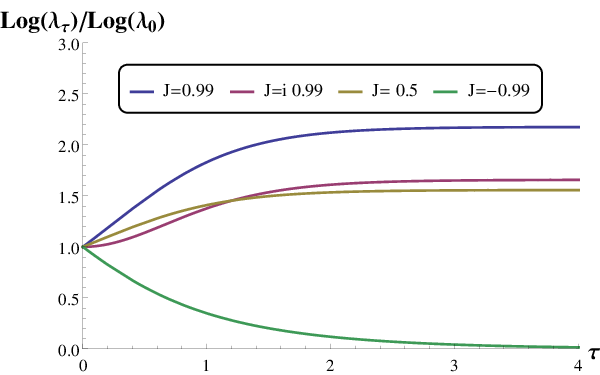
It is an amusing fact that there is a maximum value of $\theta$ given $\theta_{0}$, which corresponds to $J=\coth\tau$. For example, for infinite Euclidean time the maximum value is approximately $2.18844\theta_{0}$. For finite time, the maximum may be larger than this number, but still finite. At any time, this bound on the ratio $\theta/\theta_{0}$ of Teicmüller parameters is more stringent than the purely geometric bound coming from studying K-quasiconformal maps (see the Conclusions). So we seem to have found a new dynamical selection rule.

Note that even when $\lambda_{\tau}$ is fixed there are infinite values of $J$ that give the same value of $A$. To see the root of this issue we should remember that $\mu$ depends on $J$, but from Teichmüller theory we know that different Beltrami coefficients $\mu$, that is different $J$’s may give the same complex structure. In other words, it is the class $[\mu]$, rather than the parameter $\mu$, which defines the complex structure at time $\tau$. This is related to the discussion at the end of eq. (2.1), since the choice of reduced Teichmüller space implies that the quadratic differential $q$ should be real on the boundary in order to identify it with the fibre of the cotangent phase space, so that $J$ should also be real. This is from a 2-dimensional perspective, but from the 3-dimensional interpolating manifold, there is no reason to require a real $J$, yet it is only $\mbox{Re}\,{J}$ that parametrizes unambiguously the final complex structure. This point can be made more clear: the level sets of $A$ for given $\tau$ can be visualized in Figure 3. Each level curve of $A$ intersects the real $J$ line only once.

Let us define $\rho:=y/a$, so the metric (36) reads,

The Euclidean action, taking into account the 1/2 factor in front of the GH terms, is

The regularized range of integration of $y$ at different times is not evident so we have to assume that for small arg$(z)=y$ we have $\mbox{arg}(z)=\epsilon\cosh\tau$. This assumption is motivated by the discussion of the $\mu=0$ case done before, but it is ultimately justified from the embedding of a surface of constant $\tau$ into $\mathbb{H}^{3}/\Gamma$ ¹³¹³ 13 The embedding of constant $\tau$ surfaces in the space $\mathbb{H}^{3}/\Gamma$ for generic $J$ is quite complicated [28]. However, for purely imaginary $J$ the expressions simplify enormously (see the Appendix), and it is indeed the case that the regularizing cone implies arg$(z)=\epsilon\cosh\tau$. Figure 4 was plotted using such embedding..

The volume part is:

The one-half Gibbons-Hawking term coming from the fixed time surfaces is

We already see that the finite-term contributions cancel when we sum the bulk part plus the GH of constant-time surfaces. In contrast, the divergent part is still there, because we need to consider the rest of the boundary, namely the regulating surface contribution.

Let us consider again the cone in $\mathbb{H}^{3}$, which in canonical coordinates is defined by
$Z/\sqrt{X^{2}+Y^{2}+Z^{2}}=\sin\epsilon$. This means that, for small $\epsilon$, arg$(z)\simeq\epsilon\cosh\tau$. The induced metric, in the $(\tau,x)$ coordinates, can be obtained from the embedding in the Appendix,

This implies that the square root of the determinant is $\sqrt{h}\simeq\cosh\tau(\theta_{0}/a)\epsilon^{-1}+\mathcal{O}(\epsilon)$. The normal to the cone is $n=-\epsilon^{-1}d\epsilon$, which means Tr$K=\cos\epsilon+\sec\epsilon\simeq 2+\mathcal{O}(\epsilon^{2})$. We can now compute the GH radial term:

This term gives the exact same divergent contribution as the GH terms (45) at fixed-time surfaces, which help cancelling the $1/\epsilon$ divergence of the volume part.

Then, the on-shell action reads

We have seen that, by equation (17), there are curves in the complex $J$ plane (actually inside the disk $|J|<\coth\tau$) that are defined by the pair $(\theta_{0},\theta)$ (here $\theta$ should be thought as independent of $\theta_{0}$). These level curves were plotted in Figure 3.

Each level curve denotes a set of instantons that interpolate between the given initial and final complex structures. Having shown in the previous Section that the action of any such instanton is zero, we reach a first conclusion: processes that change the aspect ratio of the cylinder are in fact classically allowed. This agrees with the result of the analysis of the exact quantum evolution in the “constrain first” approach. The vanishing of the classical instanton action also means that the contribution to the path integral is just given by the integration measure. This object should be defined in a sensible way. For the moment, it seems reasonable to just take the Euclidean length $l_{\tau}(\theta,\theta_{0})$ of the level curve as a good measure, although we will only use it for numerical evaluation¹⁴¹⁴ 14 It is of course worth exploring the possibility of choosing other measures, but we leave this to future work.. Then

Although we are not indicating it explicitly, these lengths are a function of $\theta/\theta_{0}$. This means that the length (path integral) should be invariant under scaling $\theta\rightarrow b\,\theta$, for any real and positive $b$. This allows us to rewrite the previous equation as

To interpret this expression as a probability amplitude we should impose that the length is normalized with a scale-invariant probability measure, i.e.

By a numerical approximation it is possible to plot the normalized length, $|\langle\theta,\tau|\theta_{0},0\rangle|^{2}$, as a function of $\theta/\theta_{0}$, see Figure 5.

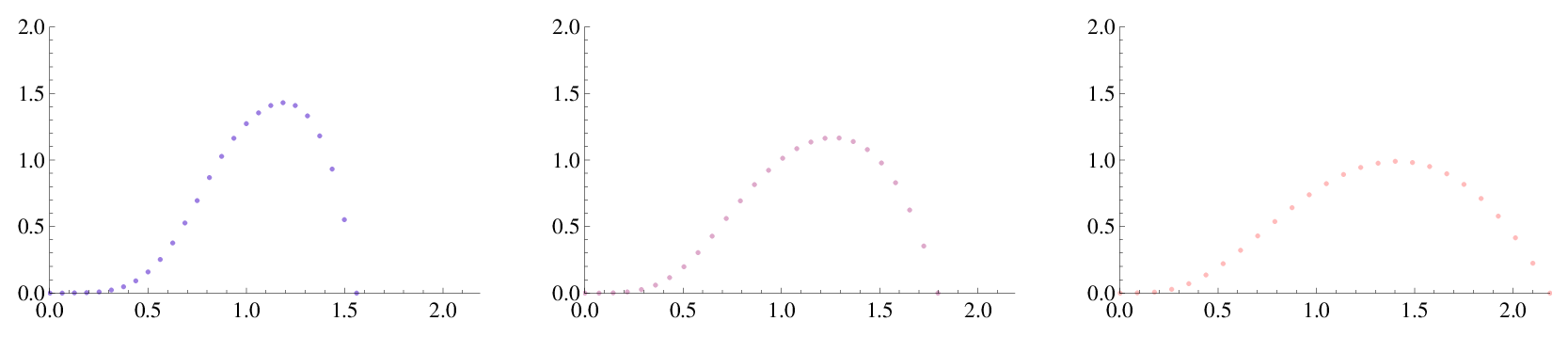
In the coordinate $x:=\log\theta$ the measure of integration $d\theta/\theta$ becomes $dx$, the only translation invariant measure in $\mathbb{R}$. The Hilbert space is of course $\mathcal{H}=\mathcal{L}^{2}(\mathbb{R},x)$.

References

- [1] S. Deser and R. Jackiw, “Three-Dimensional Cosmological Gravity: Dynamics of Constant Curvature,” Annals Phys. 153, 405 (1984); S. Deser, R. Jackiw and G. ’t Hooft, “Three-Dimensional Einstein Gravity: Dynamics of Flat Space,” Annals Phys. 152, 220 (1984);
- [2] M. Banados, C. Teitelboim and J. Zanelli, “The Black hole in three-dimensional space-time,” Phys. Rev. Lett. 69, 1849 (1992)
- [3] M. Banados, M. Henneaux, C. Teitelboim and J. Zanelli, “Geometry of the (2+1) black hole,” Phys. Rev. D 48, 1506 (1993) Erratum: [Phys. Rev. D 88, 069902 (2013)]
- [4] D. R. Brill, “Multi - black hole geometries in (2+1)-dimensional gravity,” Phys. Rev. D 53, 4133 (1996)
- [5] S. Aminneborg, I. Bengtsson, D. Brill, S. Holst and P. Peldan, “Black holes and wormholes in (2+1)-dimensions,” Class. Quant. Grav. 15, 627 (1998)
- [6] D. Brill, “Black holes and wormholes in (2+1)-dimensions,” Lect. Notes Phys. 537, 143 (2000) [gr-qc/9904083].
- [7] E. J. Martinec, “Soluble Systems in Quantum Gravity,” Phys. Rev. D 30, 1198 (1984).
- [8] A. Achucarro and P. K. Townsend, “A Chern-Simons Action for Three-Dimensional anti-De Sitter Supergravity Theories,” Phys. Lett. B 180, 89 (1986).
- [9] E. Witten, “(2+1)-Dimensional Gravity as an Exactly Soluble System,” Nucl. Phys. B 311, 46 (1988).
- [10] E. Witten, “Topology Changing Amplitudes in (2+1)-Dimensional Gravity,” Nucl. Phys. B 323, 113 (1989).
- [11] S. P. Martin, “Observables in (2+1)-dimensional Gravity,” Nucl. Phys. B 327, 178 (1989).
- [12] S. Carlip, “Exact Quantum Scattering in (2+1)-Dimensional Gravity,” Nucl. Phys. B 324, 106 (1989).
- [13] V. Moncrief, “Reduction of the Einstein equations in (2+1)-dimensions to a Hamiltonian system over Teichmuller space,” J. Math. Phys. 30, 2907 (1989).
- [14] A. Hosoya and K. i. Nakao, “(2+1)-dimensional Pure Gravity for an Arbitrary Closed Initial Surface,” Class. Quant. Grav. 7, 163 (1990).
- [15] S. Carlip, “Observables, Gauge Invariance, and Time in (2+1)-dimensional Quantum Gravity,” Phys. Rev. D 42, 2647 (1990).
- [16] J. Kim and M. Porrati, “On a Canonical Quantization of 3D Anti de Sitter Pure Gravity,” JHEP 1510, 096 (2015) doi:10.1007/JHEP10(2015)096 [arXiv:1508.03638 [hep-th]].
- [17] C. Scarinci and K. Krasnov, “The universal phase space of gravity,” Commun. Math. Phys. 322, 167 (2013) doi:10.1007/s00220-012-1655-0 [arXiv:1111.6507 [hep-th]].
- [18] K. Krasnov and J. M. Schlenker, “Minimal surfaces and particles in 3-manifolds,” Geom. Dedicata 126, 187 (2007)
- [19] S. Nag, “The complex analytic theory of Teichmüller spaces”, John Wiley, New York, Chichester, Brisbane, Toronto, Singapore (Canadian Mathematical Society Series of Monographs and Advanced Texts), 1988, ISBN 0-471-62773-9 .
- [20] F. P. Gardiner, Quasiconformal Teichmüller Theory, American Mathematical Society (2000).
- [21] V.I. Arnold, Geometrical Methods in the Theory of Ordinary Differential Equations, Springer (2012).
- [22] J. B. Hartle and S. W. Hawking, “Wave Function of the Universe,” Phys. Rev. D 28, 2960 (1983) [Adv. Ser. Astrophys. Cosmol. 3, 174 (1987)].
- [23] L. V. Ahlfors, “Lectures on quasiconformal mappings” , University Lecture Series, vol. 38 (2006).
- [24] K. Krasnov, “Holography and Riemann surfaces,” Adv. Theor. Math. Phys. 4, 929 (2000)
- [25] L. A. Takhtajan and L. P. Teo, “Liouville action and Weil-Petersson metric on deformation spaces, global Kleinian reciprocity and holography,” Commun. Math. Phys. 239, 183 (2003)
- [26] M. T. Anderson, “On quasi-local Hamiltonians in General Relativity,” Phys. Rev. D 82, 084044 (2010)
- [27] E. Witten, “A Note On Boundary Conditions In Euclidean Gravity,” arXiv:1805.11559 [hep-th].
- [28] A. Garbarz, J. Kim and M. Porrati, Work in progress.