Geometrically finite
transcendental entire functionsThanks: The first author thanks Princess Nora bint Abdulrahman University in Saudi Arabia for supporting her doctoral studies at the University of Liverpool.
University of Liverpool
Liverpool L69 7ZL
UK
![[Uncaptioned image]](2003.08884v3/orcid2.png) https://orcid.org/0000-0001-8032-8580
Email address: l.rempe@liverpool.ac.uk
Dave Sixsmith
Address: Dept. of Mathematical Sciences
https://orcid.org/0000-0001-8032-8580
Email address: l.rempe@liverpool.ac.uk
Dave Sixsmith
Address: Dept. of Mathematical Sciences
University of Liverpool
Liverpool L69 7ZL
UK
https://orcid.org/0000-0002-3543-6969
Email address: david.sixsmith@open.ac.uk
Abstract.
For polynomials, local connectivity of Julia sets is a much-studied and important property. Indeed, when the Julia set of a polynomial of degree is locally connected, the topological dynamics can be completely described as a quotient of a much simpler system: angle -tupling on the circle.
For a transcendental entire function, local connectivity is less significant, but we may still ask for a description of the topological dynamics as the quotient of a simpler system. To this end, we introduce the notion of docile functions (Definition 1.1): a transcendental entire function with bounded postsingular set is docile if it is the quotient of a suitable disjoint-type function. Moreover, we prove docility for the large class of geometrically finite transcendental entire functions with bounded criticality on the Julia set. This can be seen as an analogue of the local connectivity of Julia sets for geometrically finite polynomials, first proved by Douady and Hubbard, and extends previous work of the second author and of Mihaljević for more restrictive classes of entire functions.
We deduce a number of further results for geometrically finite functions with bounded criticality, concerning bounded Fatou components and the local connectivity of Julia sets. In particular, we show that the Julia set of the sine function is locally connected, answering a question raised by Osborne.
2010 Mathematics Subject Classification
Primary 37F10; Secondary 30D05, 30F45, 37F20.1. Introduction
Suppose that is an entire function, and denote by the th iterate of . The Fatou set consists of those points where the dynamics of is “regular”, or, more precisely, where the iterates form a normal family. Its complement is the Julia set ; it is the locus of “chaotic” behaviour.
Let be a polynomial of degree with connected Julia set. By the Riemann mapping theorem there is a conformal isomorphism mapping the complement of the unit disc in the Riemann sphere to the attracting basin of infinity for , in such a way that . This isomorphism is in fact a conjugacy between and the action of [Mil06, Theorem 9.5].
If extends continuously to the unit circle, then the extension is a semiconjugacy between the action of on the circle (i.e., angle -tupling) and the action of on its Julia set. Therefore we obtain a complete description of the interesting topological dynamics of . By a classical theorem of Carathéodory and Torhorst [Car13, Tor21], such a continuous extension exists if and only if is locally connected; see [Pom92, Theorem 2.1]. It is for this reason that local connectivity of Julia sets is one of the central topics of study in polynomial dynamics. Many, but not all, polynomial Julia sets are locally connected; see e.g. [Mil00] for a discussion.
The study of the dynamics of transcendental entire functions has also received considerable attention. Here infinity is an essential singularity, rather than an attracting fixed point, and the escaping set , consisting of points whose orbits under converge to this singularity, is no longer open. Furthermore, the set of singular values , which generalises the set of critical values of a polynomial, may be very complicated.
The Eremenko-Lyubich class consists of those transcendental entire functions for which is bounded; see [EL92, Six18]. It is characterised by strong expansion properties near infinity [EL92, Lemma 1], which in turn lead to a certain rigidity of the structure of the set [Rem09]. As discussed above, many methods in the polynomial setting rely on studying the dynamics via structures in the escaping set. Therefore the class is perhaps the best setting for adapting these methods to transcendental entire functions – despite the major differences that remain.
A function in is said to be of disjoint type if its Fatou set is connected and compactly contains the postsingular set. (Recall that the postsingular set is the closure of the forward orbit of the set of singular values.) The dynamical properties of these maps were studied in detail in [Rem16], which gave a comprehensive topological description of their Julia sets.
It is natural to consider functions of disjoint type to be the simplest maps in their given parameter space. Here by the parameter space of a map , we mean the class of all entire functions that are quasiconformally equivalent to . In other words, they are obtained from by pre- and post-composition with quasiconformal homeomorphisms; see, for example, [Rem09, p. 245]. It is straightforward to show that if , then is of disjoint type for all sufficiently small values of [BK07, p.392]; in particular, every such contains a disjoint-type function in its parameter space. Moreover, any two quasiconformally equivalent functions of disjoint type are quasiconformally conjugate on their Julia sets [Rem09, Theorem 3.1].
So we may consider a function of disjoint type to play the same role for its parameter space as does for polynomials of degree . It appears natural to ask for which the dynamical properties of the disjoint type function can be “transferred” to the original map using a semiconjugacy from the Julia set of to that of .
The first general result in this direction was given in [Rem09, Theorem 1.4], which states that such a semiconjugacy can be constructed for all hyperbolic functions. (A transcendental entire function is hyperbolic if is compact, and is empty; see [RS17].) This result was extended by Mihaljević [Mih12], who showed that such a construction is possible for a larger class of functions she calls strongly subhyperbolic. Here a transcendental entire function is called subhyperbolic if the set is compact, and is finite. It is called strongly subhyperbolic if, in addition, has bounded criticality on the Julia set; that is, contains no finite asymptotic values of , and the local degree of at the points in is uniformly bounded. It is easy to see that the result becomes false in general when there are asymptotic values in the Julia set. In fact, even for the postsingularly finite function , many questions about the topological dynamics remain unanswered; see [Wor18].
Given the fundamental importance that local connectivity of the Julia set plays for polynomials, it seems desirable to define an analogue of this notion for transcendental entire functions, by formalising the desired properties of the semiconjugacy above. This is the first aim of our article. Let be a function with bounded postsingular set , and let be sufficiently small to ensure that is of disjoint type. It follows from the results of [Rem09] that there is a natural (but not necessarily continuous) bijection between the escaping sets of and ; see [BR20, Section 7] and Section 2 below. (Recall that a point belongs to the escaping set if its orbit tends to infinity.)
We may think of as an analogue of the Riemann map in the case of polynomials. Hence the following definition makes sense as an analogue of local connectivity of the Julia set.
1.1 Definition (Docile functions).
The postsingularly bounded function is called docile if the bijection extends to a continuous function
With this new terminology, we may state the main result of Mihaljević in [Mih12] as follows.
1.2 Theorem.
A strongly subhyperbolic entire function is docile.
A particularly important class of polynomials consists of those for which each critical point in the Julia set has a finite orbit; see, for example, [CG93, Theorem 4.3] and [McM00]. These maps are called geometrically finite. The natural extension of this definition to transcendental entire functions was given by Mihaljević [Mih10]. We say that a transcendental entire function is geometrically finite if is compact and is finite. We also say that is strongly geometrically finite if it is geometrically finite with bounded criticality on the Julia set. As noted in [Mih10], all subhyperbolic maps are geometrically finite, while a geometrically finite map is subhyperbolic if and only if it has no parabolic orbits. Clearly all geometrically finite maps are in the class . Our main result is the followin extension of Theorem 1.2.
1.3 Theorem.
A strongly geometrically finite entire function is docile.
An immediate consequence can be stated more directly.
1.4 Corollary (Semiconjugacies for geometrically finite functions).
Suppose that is strongly geometrically finite, and that is such that the map is of disjoint type. Then there exists a continuous surjection , such that:
- (a)
;
- (b)
;
- (c)
is a homeomorphism and ;
- (d)
For each component of the map is a homeomorphism.
Remark.
The key idea of the proof of Theorem 1.2 given in [Mih12] is to show that is uniformly expanding near the Julia set, with respect to a certain orbifold metric. The desired semiconjugacy is then obtained by a standard construction: for a point , we iterate forward steps under , then pull back the resulting point times under , using appropriate branches. The uniform expansion property ensures that this process converges, and that depends continuously on . See also [Par19], in which the orbifold metric is used in a similar way to study a class of maps for which the postsingular set is unbounded.
When has parabolic orbits, the function cannot be uniformly expanding near the parabolic point for any metric, and new techniques are required. The crux of the argument in this paper is to modify a suitable orbifold metric in a neighbourhood of each parabolic cycle in such a way that there is still sufficient expansion for the construction to converge. This idea is also used in the proof of local connectivity of the Julia set of a geometrically finite polynomial; see, for example, [CG93, Theorem 4.3], and [TY96] which studies the case of a geometrically finite rational map. However, there are additional challenges to overcome in the transcendental case. In particular, the proofs in the polynomial and rational case obtain uniform expansion arguments near pre-images of parabolic points by relying, in an essential way, upon the fact that the degree of is finite, and therefore there are only finitely many such points. A new argument is needed for transcendental entire functions. (Compare the remarks in the proof of Proposition 7.1.)
Docile functions have many strong dynamical properties, which will be explored in a subsequent paper. Here, we give three simple examples of such properties in our setting. Recall that a Cantor bouquet is a certain type of uncountable union of arcs to infinity, called hairs, and a pinched Cantor bouquet is the quotient of a Cantor bouquet by a closed equivalence relation defined on its endpoints, embedded in a plane in a way that preserves the cyclic ordering of its hairs at infinity. Compare [Mih12, BJR12]. The following result then follows from Corollary 1.4 and [BJR12].
1.5 Corollary (Pinched Cantor Bouquets).
Suppose that is strongly geometrically finite, and that additionally is either of finite order, or a finite composition of class functions of finite order. Then is a pinched Cantor bouquet.
The second result also follows immediately from Corollary 1.4, together with well-known properties of disjoint-type functions.
1.6 Corollary (Components of the escaping set).
Suppose that is strongly geometrically finite. Then has uncountably many connected components.
Remark.
For , which is subhyperbolic but has an asymptotic value in the Julia set, the escaping set is connected [Jar11]. It is conjectured that, in general, the escaping set of a transcendental entire function is either connected or has uncountably many components; see [RS19] for a partial result in this direction.
Our third result concerns the case that the Fatou set of a geometrically finite map is connected.
1.7 Theorem (Geometrically finite maps with connected Fatou set).
Suppose that is geometrically finite, and that is connected and non-empty. Then is strongly geometrically finite, and the function in Corollary 1.4 is a homeomorphism between and . In particular, if is either of finite order, or a finite composition of class functions of finite order, then is a Cantor bouquet.
In [BFR15] the uniform expansion property of hyperbolic maps was used to study the Fatou and Julia sets of these functions. The results of that paper included various sufficient conditions for all Fatou components to be bounded, and other sufficient conditions for the Julia set to be locally connected. Using the expansion properties for strongly geometrically finite functions obtained in the course of the proof of Theorem 1.3, we are able to deduce that many of the results of [BFR15] can be generalised to this larger class. We give two such results. The first concerns the boundedness of the components of the Fatou set, and is a generalisation of [BFR15, Theorem 1.2].
1.8 Theorem (Bounded Fatou components).
Suppose that is strongly geometrically finite. Then the following are equivalent:
- (a)
every component of is a bounded Jordan domain;
- (b)
the map has no asymptotic values, and every component of contains at most finitely many critical points.
The second result concerns the local connectedness of the Julia set, and generalises [BFR15, Corollary 1.8].
1.9 Theorem (Bounded degree implies local connectivity).
Suppose that is strongly geometrically finite with no asymptotic values. Suppose, furthermore, that there is a uniform bound on the number of critical points, counting multiplicity, that are contained in any single Fatou component of . Then is locally connected.
As in [BFR15, Corollary 1.9(a)], when each Fatou component contains at most one critical value, Theorem 1.9 implies the following.
1.10 Corollary (Locally connected Julia sets).
Suppose that is strongly geometrically finite with no asymptotic values, and that every component of contains at most one critical value. Suppose additionally that the multiplicity of the critical points of is uniformly bounded. Then is locally connected.
The function has a triple fixed point at the origin, and each of the two immediate parabolic basins contains one of the two critical values . Hence Corollary 1.10 gives a positive answer to Osborne’s question [Osb13, remark following Example 6.2] whether is locally connected. See Example 11.2 and Figure 3 below.
Remark.
Finally, we discuss some further consequences of Theorem 1.3. The exponential family consists of the maps
| (1.1) |
The strongly geometrically finite exponential maps are exactly those that have either an attracting or a parabolic orbit. For this setting, Corollary 1.4 was stated in [Rem06], but the proof was given only for the case of attracting orbits.
The simplest geometrically finite map in this family that is not also subhyperbolic is , which has a parabolic fixed point at and connected Fatou set; see Example 11.1 below. For this function, it was observed by Devaney and Krych [DK84] that the Julia set is an uncountable collection of arcs to infinity. Furthermore, Aarts and Oversteegen [AO93] proved that the Julia set of is a Cantor bouquet. It follows from Theorem 1.7 that, indeed, is topologically conjugate to any disjoint type exponential map on its Julia set, for example to .
These results are related to the following more general phenomenon. Suppose that is a polynomial, or even a rational function, that is geometrically finite. Then it is possible to perturb such that all parabolic orbits become attracting, without changing the topological dynamics on the Julia set. More precisely, there is a path in the space of geometrically finite rational functions of the same degree, ending at , such that each is conjugate to on its Julia set, and has no parabolic cycles. Furthermore, the conjugacy depends continuously on and tends to the identity as tends to along . See [CT18], [Ha98, Ha00, Ha02] and [Kaw03, Kaw06] for more details.
It seems likely that, using our techniques, these results can be extended to the case of strongly geometrically finite functions. Here, we restrict ourselves to noting a direct consequence of Theorem 1.3. Suppose that and are two strongly geometrically finite functions in the same quasiconformal equivalence class, and suppose that and are disjoint-type functions with and , for some . Let be the semiconjugacy between and from Corollary 1.4. Note that and are quasiconformally equivalent and hence, by [Rem09, Theorem 3.1], quasiconformally conjugate. So there is also a semiconjugacy between and . Suppose that we can additionally conclude, say by combinatorial means, that the identifications between non-escaping points of induced by are the same as those induced by . Then and are are conjugate on their Julia sets, since they are, topologically, the quotient of the same map, by the same equivalence relation.
In particular, using prior results from [RS08], we can conclude the following for the case of exponential maps as defined in (1.1). A hyperbolic component is a connected component of the set of parameters such that is hyperbolic. The hairs or external rays of an exponential map are the path-connected components of the escaping set ; these hairs are ordered “vertically” according to how they tend to infinity; compare [RS08, Section 2].
1.11 Theorem (Conjugate exponential maps).
Suppose that is a parameter such that has a parabolic cycle. Then there exists a unique hyperbolic component such that, for , the functions and are topologically conjugate when restricted to their respective Julia sets, by a conjugacy that respects the vertical order of hairs. Moreover, .
Structure
We now discuss the structure of this paper, including a brief outline of the proof of Theorem 1.3, which is long and quite complicated. We begin by discussing docility, and the natural bijection between escaping sets, in more detail in Section 2. In particular, Proposition 2.3 establishes a number of important properties of the semiconjugacy for docile functions in general, and thus reduces the proof of Corollary 1.4 to the proof of Theorem 1.3. The discussion also sets the stage for the proof of Theorem 1.3.
Next, we present some preliminaries for the construction of an expanding metric. Section 3 discusses the dynamics of an entire function near a parabolic point; Section 4 gives an introduction to Riemann surface orbifolds. We collect basic results concerning geometrically finite functions in Section 5.
The proof of Theorem 1.3 proceeds, very roughly, as follows. Suppose that is strongly geometrically finite. In order to obtain expansion estimates in the repelling directions of parabolic periodic points, we must work with an iterate of . Specifically, we choose the smallest value such that all parabolic points of the map are fixed and of multiplier one. Note that and have the same Julia set, Fatou set and parabolic periodic points; we shall use these facts without comment. It is not difficult to verify that is also strongly geometrically finite.
In the polynomial case, the analogous property to docility (continuous extension of the Riemann map) can be expressed in terms of a topological property of the Julia set (local connectivity), and therefore it holds for if and only it holds for any iterate. For transcendental entire functions, it is less straightforward to see that docility of implies docility of . Hence we instead prove docility of the original function directly, but using expansion extimates only known to hold for the iterate . This is another subtle difference between the proofs in the polynomial and transcendental cases.
More precisely, in Section 6 we construct certain hyperbolic orbifolds , and such that the maps and are orbifold covering maps. This construction is closely related to that in [Mih12]. In Section 7 we modify the orbifold metric on close to the parabolic fixed points of . The modification itself is modelled on that used in the rational case, but a new argument is required in order to show that expands this metric uniformly away from parabolic points. In Section 8, we combine the results of the previous section with known estimates near parabolic points, in order to obtain a suitable global estimate. In Section 9, we use this expansion to prove Theorem 1.3. We also give the proofs of Theorem 1.7 and Theorem 1.11.
Notation and terminology
We denote the Riemann sphere by , and the unit disc centred at the origin by . The (Euclidean) open ball of radius around a point is denoted by
Unless stated otherwise, topological operations such as closure are taken in the plane. If , then we write if the closure of is compact and contained in . We denote the Euclidean distance between two sets by dist. When is the singleton we just write dist.
We refer to [Ber93, Sch10] for background on transcendental dynamics. Also see [Six18] for background on the Eremenko-Lyubich class , as well as for elementary definitions and properties used in this paper, which we omit for reasons of brevity.
Suppose that is a transcendental entire function. We denote by and the set of attracting and parabolic periodic points, respectively. We let denote the union of attracting Fatou components; i.e., the set of points whose orbit converges to an attracting periodic orbit. The set is defined analogously. For we define .
2. Docile functions
Let be a transcendental entire function with bounded postsingular set , and let be sufficiently small to ensure that is of disjoint type. As mentioned in the introduction, there is a natural bijection . This bijection arises from a certain conjugacy between and on the set of points whose orbits remain close to infinity, as constructed in [Rem09]. The existence of this bijection is implicit in [Rem07, Proof of Theorem 3.5], but is first made explicit in [BR20, Proof of Theorem 7.2]. Here, we give a slightly different description, for suitably small , which avoids “external addresses”, which are used in [BR20]. The construction will also allow us to explain the strategy of the proof of Theorem 1.3.
We begin by choosing a value of . Choose sufficiently large that
| (2.1) |
Set , and consider defined as above. Then . Furthermore,
Hence is contained in the immediate basin of an attracting fixed point of , and is of disjoint type; compare also [Mih12, Proposition 2.8].
Next we define
By construction for all , and , for . Since every point in the Fatou set eventually iterates into , we deduce that
We now construct a sequence of conformal isomorphisms
| (2.2) |
such that
| (2.3) |
We first set and , and note that (2.2) and (2.3) both hold with . Also observe that is defined on and takes values in there. Consider the isotopy
between and on . Since is a covering map, lifts to an isotopy on between and a map . The restriction of to takes values in and satisfies (2.3) by construction. We continue this procedure inductively to define for all . Observe that each extends to a homeomorphism
with .
Let be a connected component of . Then, for , there is a unique connected component of such that . Consider the connected components of , for . It follows from the construction that all sufficiently large points of also lie in . We say that tends to in . If , then is injective, and hence is the unique connected component of that tends to infinity within .
The following is a consequence of [Rem09, Section 3] and [BR20, Proposition 4.4]. Let us denote by the set of all points of whose orbits do not enter the disc .
2.1 Theorem (Conjugacy near infinity).
There is such that the restrictions converge uniformly in the spherical metric to a function
which is a homeomorphism onto its image, and satisfies on .
For sufficiently large , . Moreover, let and denote the connected component of containing by . Then, for , tends to infinity within , and the unbounded connected component of contains , as well as for .
As mentioned in the introduction, this result leads to the existence of a natural bijection between escaping sets.
2.2 Theorem (Natural bijection).
For every , the values converge to a limit . The function is a bijection, and satisfies .
Proof.
Let be as in Theorem 2.1. Let , and write . For and , let be the connected component of such that
That is, if is the connected component of containing , then . In particular, tends to infinity within . Let denote the unbounded connected component of .
Since , there is such that . Then, by Theorem 2.1, the sequence converges to a point . Moreover, by the final statement of the theorem, and belong to the same connected component of for . In other words, , and we see that for .
The function maps conformally to a component of . By the functional relation (2.3),
So , and is a conformal isomorphism. It follows that for .
Inductively we see that is a conformal isomorphism for , with . Let
be the corresponding branch of . Since is also a subset of , it follows that on .
Hence we see that
for all . In particular, converges to . Setting , we have proved the existence of the limit function , which satisfies the desired functional relation by (2.3).
It remains to show that the map is a bijection. Firstly suppose that with . Let be chosen sufficiently large that . Then
Since the restriction of to is injective, we see that .
Now use the same notation as above. Then is the component of containing , and is the component of containing , with . Let and be the components of containing and , respectively. By construction, we have
So . As is injective, we conclude that , as desired.
Similarly, let , and write . By Theorem 2.1, there is and such that . Let and be as above, and set
Then , and is a conformal isomorphism by the functional relation (2.3). Let be the unique point with . According to the construction of in the first part of the proof, is the unique point in with . Thus and is surjective, as claimed. ∎
Recall from the introduction that is said to be docile if the bijection is continuous and extends to a continuous function on . Observe that is not, strictly speaking, canonical, as we could have chosen a different isotopy between and , leading to a different choice of . Moreover, the initial choice of and provides a “quasiconformal equivalence” between and ; there may be other such equivalences which can be used for the same purpose. However, using the results of [Rem09], it can be shown that any two possible bijections that arise in this manner differ by a quasiconformal self-conjugacy of on its Julia set, much in the same way that the Böttcher map for a polynomial of degree is defined only up to multiplication with a -th root of unity. Similarly, a different choice of , and hence of , will lead to the same function , up to a quasiconformal conjugacy between the corresponding disjoint-type functions on their Julia sets. In particular, the definition of docility is independent of these choices.
Properties of docile functions will be studied in greater detail in a forthcoming separate article. Here, we restrict to showing that, for a docile function , the conjugacy necessarily has the properties stated in Corollary 1.4.
2.3 Proposition (Semiconjugacies for docile functions).
Let , and be as above. Suppose that is docile. Then the continuous extension has the following properties.
- (a)
.
- (b)
is surjective onto .
- (c)
and on .
- (d)
is a homeomorphism and .
- (e)
For each component of the map is a homeomorphism.
Proof.
In the following, let us write , and similarly for . By Theorem 2.2, is a bijection between and . Since is dense in , and is compact, it follows that is indeed surjective onto , establishing b.
To prove c, let , and let be a sequence converging to . Set and ; so . If , then we have
| (2.4) |
Conversely, if , then . Hence the set
is backwards-invariant. The Julia set of the disjoint-type function contains no Fatou exceptional points, and hence the backwards orbit of any is dense in . As is closed in , we have either or . The latter is impossible since maps to .
As for d, we already know that is a continuous bijection. Moreover, by compactness of , together with a and c, we have
for any sequence in . In particular, . It remains to show that the inverse of the restriction is continuous. This is a consequence of the following fact: If is a continuous surjection between compact metric spaces, and is injective for some , then this restriction is a homeomorphism. See e.g. [Kah98, Lemma 2.2.13].
Finally, we prove e. Let be a connected component of . Since is compact, it remains to show that is injective on the set of non-escaping points in . So let with , and set , . By assumption, there is a subsequence such that . On the other hand, we have
as ; see e.g. [RRRS11, Lemmas 3.1 and 3.2]. In particular, . So , while does not accumulate on by c. So for sufficiently large ; by the semiconjugacy relation, this implies , as claimed. ∎
We conclude the section by observing that, in order to establish docility, it is enough to see that the maps converge uniformly.
2.4 Observation.
If the convergence of is uniform with respect to the spherical metric, then is docile.
Proof.
Recall that is defined and continuous on . Since converges uniformly on , and is dense in , the sequence is Cauchy on . Therefore it converges uniformly to a continuous function as desired. ∎
In [Rem09, Section 5] and [Mih12], this is in fact how the semiconjugacy is constructed: expansion in a suitable hyperbolic metric is used to establish uniform convergence of the . As mentioned in the introduction, we follow the same strategy, but need to take particular care about the definition of the metric near parabolic points.
3. Parabolic periodic points
In this section, we collect some local results concerning parabolic points. These are well-known, but we know of no reference that contains them precisely in the form that we require.
Recall that a periodic point of period is parabolic if
The orbit is called a parabolic cycle. If we replace with a sufficiently large iterate, then we obtain
and now we say that is a multiple fixed point.
We begin with some definitions and results relating to a function , analytic in a neighbourhood of the origin, such that the origin is a multiple fixed point. All definitions and results we give here can be transferred to the original function by a conjugacy; we usually do so without comment. We can assume that is sufficiently small that has a well-defined and analytic inverse on . For more background on the dynamics of an analytic function in a neighbourhood of a parabolic fixed point, we refer to, for example, [Bea91, Mil06].
Note first that there exist and such that
| (3.1) |
Here is termed the multiplicity of the parabolic fixed point.
The dynamics of are determined by attracting and repelling vectors, which are defined as follows. A repelling vector is a complex number such that , and an attracting vector is a complex number such that .
Following [Mil06, Section 10], if is a parabolic fixed point of multiplier one and multiplicity , and is an attracting vector at , then we say that the orbit of a point converges to in the direction if as . We shall work with “petals” around the attracting (and repelling) directions that are sufficiently “thick”, in the following sense.
3.1 Proposition (Attracting petals).
Suppose that is a neighbourhood of the origin, that is an analytic function on , and that the origin is a multiple fixed point, with attracting vector and of multiplicity . Suppose finally that . Then there exist a Jordan domain and such that
- (a)
;
- (b)
if , then the orbit of converges to in the direction if and only if for all sufficiently large values of ;
- (c)
.
Proof.
We can suppose that has the form (3.1). To conjugate to a function which is close to near infinity, we define functions
| (3.2) |
defined in a neighbourhood of . It is elementary to see that there is a function , defined on a neighbourhood of , such that
| (3.3) |
Shrinking and restricting if necessary, we may assume that is defined on . A calculation shows that
| (3.4) |
We call an attracting petal for (of opening angle at least ) at . We also call the set an attracting sector of angle and radius . The corresponding sets for the inverse are called repelling petals and repelling sectors, respectively.
We will need to work with repelling sectors that are “thin”, in the sense that their opening angle is sufficiently small. To be definite, let be a repelling vector, and let us call the sector a thin repelling sector. (The angle could be replaced by any number strictly less than in the following.)
The reason for this terminology is that we have good control of and its derivative in a thin repelling sector.
3.2 Proposition (Thin repelling sectors).
Suppose that is a neighbourhood of the origin, that is an analytic function on , that the origin is a multiple fixed point of , and that is a repelling vector of at . Then there exists such that
| (3.5) |
Moreover, if is such that lies in a thin repelling sector , then .
Proof.
Without loss of generality, we can assume that the argument of the repelling vector is zero. Let the multiplicity of the parabolic fixed point be . It follows that there exists such that, as ,
Since is real and positive and, by assumption, , the first part of (3.5) is immediate, as is the final claim of the proposition.
We also need to know that, when some number of iterates stay within the same thin repelling sector, the derivative of grows sufficiently quickly.
3.3 Proposition (Cascades within repelling sectors).
Suppose that is a neighbourhood of the origin, that is an analytic function on , and that the origin is a multiple fixed point of of multiplicity . Let be a repelling vector at the origin for . Then there exists with the following property. If , and is such that , for , then
| (3.6) | ||||
| (3.7) |
where are constants independent of .
Proof.
Recall that has the form (3.1), and that is the number of repelling vectors of at the origin. By Proposition 3.1, let be a repelling petal at the origin in direction , which contains a repelling sector .
We begin by fixing . By [Mil06, Theorem 10.9], there is a conformal map , known as the Fatou coordinate, such that
| (3.8) |
Let and be as defined in (3.2) and (3.3). Let be the branch of that maps a left half-plane , with , into . Set
| (3.9) |
The conformal map is known as the Fatou coordinate at infinity. Note that it follows from (3.8) that
| (3.10) |
and so, if ,
from which we deduce that
| (3.11) |
By (3.4) we can choose sufficiently small that
| (3.12) |
Set . We can then fix sufficiently small that, for the thin repelling sector , we have
This completes our choice of .
Our next goal is to find an estimate on the derivative of the Fatou coordinate at infinity; see (3.15) below. Suppose that . Define a map by
| (3.13) |
Then is a conformal map on such that and . An application of the Koebe distortion theorem gives that
| (3.14) |
By (3.12), we have that . Substituting in (3.13) and (3.14) then gives that
Hence, by (3.10), we deduce that
| (3.15) |
This is the required estimate on the derivative of .
We now use the estimate (3.15) to prove our result. Suppose that , and also that is such that , for . Let . By the choice of , and by assumption, we have . It follows by (3.11) and (3.15) that
By the definitions (3.2) and (3.3), we conclude that
This establishes (3.6). Furthermore, it follows from (3.12) that
Since , we have Re , and deduce that
and hence
as desired. ∎
We can combine the above results as follows, to obtain a statement for a global entire function having (possibly several) multiple fixed points. For reasons that will become apparent later, it will be convenient to measure expansion near the parabolic points with respect to a metric whose density is given by
| (3.16) |
where is a parameter, .
3.4 Proposition (Behaviour near multiple fixed points).
Suppose that is a transcendental entire function with finitely many parabolic points, all of which are multiple fixed points. Let . Then there exist , , and with the following properties. Consider a thin repelling sector , for a repelling vector at a multiple fixed point . Then
- (a)
We have that
- (b)
Suppose that is such that lies in a thin repelling sector of radius . Then .
- (c)
Suppose that , and are such that , for . Then
Remark.
We remark that only the values and depend on the choice of .
Proof of Proposition 3.4.
The proposition follows easily by applying the preceding results separately at each of the finitely many multiple fixed points of , and its finitely many repelling directions. Note that a follows from Proposition 3.2, since
for the parabolic point closest to , provided was chosen sufficiently small. Similarly, c follows from Proposition 3.3. Indeed, let us set and , with as above. Then
where is the multiplicity of the fixed point . So the claim follows with and , where is the maximal multiplicity of a fixed point of . ∎
4. Riemann orbifolds
In general, an orbifold is a space locally modeled on the quotient of an open subset of by the linear action of a finite group; see [Thu79, §13]. In this paper we will use the following definition, which is rather more specialised.
4.1 Definition.
An orbifold is a pair , where is a Riemann surface and a map such that is a discrete set. The map is called the ramification map. A point such that is called a ramified point.
Note that may be disconnected, in which case properties such as the type of the surface are understood component by component.
Suppose that are Riemann surfaces, and that is holomorphic. The map is called a branched covering if each point of has a neighbourhood with the property that maps each component of onto as a proper map. We wish to define holomorphic and covering maps of orbifolds. This requires the following definitions.
4.2 Definition.
Suppose that is a holomorphic map of Riemann surfaces. If , then the local degree of at , which we denote by deg, is the value such that, in suitable local coordinates,
where . In particular, is a critical point of if and only if deg.
4.3 Definition.
Suppose that is a holomorphic map of Riemann surfaces, and that and are orbifolds.
- •
The map is holomorphic if
- •
The map is an orbifold covering if is a branched covering, and
- •
If is an orbifold covering and is simply connected, then we call a universal covering orbifold of .
Every Riemann surface has a universal cover that is conformally equivalent to either or . The same is true for almost all orbifolds; see [McM94, Theorem A2]. With two exceptions (which do not occur in this paper) each orbifold has a universal cover whose underlying surface is either or . In these cases we say the orbifold is elliptic, parabolic or hyperbolic respectively. All orbifolds considered in this paper are hyperbolic, so we restrict to this case.
Denote by the unique complete conformal metric of constant curvature . Since this metric is invariant under conformal automorphisms, it descends to a well-defined metric on . We call this metric the orbifold metric, and denote it by . For simplicity we will omit the , but still refer to as the metric. If is hyperbolic, is identically one on , and , then the usual universal cover of as a Riemann surface is also a holomorphic covering map of orbifolds, and hence is identical to the hyperbolic metric in . On the other hand, becomes infinite at any ramified point.
The well-known Pick Theorem for hyperbolic surfaces generalizes to hyperbolic orbifolds [Thu84, Proposition 17.4].
4.4 Proposition.
Suppose that is a holomorphic map between hyperbolic orbifolds. Then distances, as measured in the hyperbolic orbifold metric, are strictly decreased, unless is an orbifold covering map in which case is a local isometry.
The next result follows by applying Proposition 4.4 to the inclusion map.
4.5 Corollary.
Suppose that are hyperbolic orbifolds with metrics and respectively. Suppose also that , and that the inclusion is holomorphic. Then
We also use the following observation, which gives us a form of expansion for certain orbifold coverings; this is [Mih12, Proposition 3.1].
4.6 Proposition.
Suppose that are hyperbolic orbifolds such that , and with metrics and respectively. Suppose that is an orbifold covering map, and that the inclusion is holomorphic but not an orbifold covering. Then
In order to prove an important expansion result, see Proposition 6.2 below, we require two preliminary results. The first is [BR20, Lemma 3.2].
4.7 Lemma (Preimages in annuli).
Let be an entire transcendental function which is bounded on an unbounded connected set. Let . Then, for all , and all sufficiently large , contains a point of modulus between and .
Remark.
If belongs to the unbounded connected component of , then the conclusion holds even for the preimage of the single point ; compare the proof of [Rem09, Lemma 5.1].
The second result is a generalisation of statements at the start of the proof of [Mih12, Theorem 4.1].
4.8 Proposition.
Let be a hyperbolic orbifold with such that and the set of ramified points in are both bounded. Suppose furthermore that is another orbifold with , and that for some and every sufficiently large for which , this annulus contains a ramified point with even. Then
Remark.
It is likely that the condition that be even can be omitted, but it is easy to satisfy in our context, and leads to a simple proof.
Proof.
The assumption implies that there is a sequence with , such that each is either in , or is even. Let be the orbifold , where
Then the inclusion map from to is holomorphic. It follows by [Mih12, Theorem 4.3], together with Corollary 4.5, that
We next estimate the metric in . By assumption, there is a disc such that and , for . Once again by Corollary 4.5, we can estimate above by the hyperbolic density on , which can be computed explicitly (see e.g. [Hay89, Example 9.10]). It follows that
Combining these two estimates gives
5. Dynamics of geometrically finite maps
In this section we give three general results about the dynamical properties of geometrically finite maps. The first is [Mih09, Proposition 3.1]. Here, and throughout this paper, by Jordan domain we always mean a simply-connected complementary component of a Jordan curve on the sphere; so a Jordan domain may be bounded or unbounded. Also, if and , then we define the forward orbit of by .
5.1 Proposition (Absorbing domains in attracting Fatou components).
Suppose that is a transcendental entire function, and also that is compact. Then there exist pairwise disjoint bounded Jordan domains with pairwise disjoint closures such that if , then
We also need the following, which is an analogous result for parabolic cycles.
5.2 Proposition (Absorbing domains in parabolic Fatou components).
Suppose that is a transcendental entire function with finitely many parabolic points. Suppose also that is compact. Then there exist bounded Jordan domains such that if , then the following all hold.
- (a)
.
- (b)
.
- (c)
.
- (d)
.
- (e)
If , then is an attracting petal for .
- (f)
The sets are pairwise disjoint.
- (g)
There exists with the following property. If is such that , then belongs to a thin repelling sector of .
Proof.
The proof of this result is almost exactly as the proof of [Mih09, Proposition 3.2]. Indeed, parts a, c and d are already explicitly stated in that result, and parts b, e and f are implicit in the construction in [Mih09]. (It should be noted that in [Mih09] the domains are only stated to be simply-connected, but it is easy to see that we can shrink them and obtain Jordan domains with the same property; even Jordan domains whose boundary is analytic except possibly at the parabolic points.)
That leaves only part g. This can be obtained by a very small modification to the proof of [Mih09, Proposition 3.2]. That proof uses [Mil06, Theorem 10.7] to obtain attracting petals which are contained in the domains contained in the immediate attracting basins of the parabolic fixed points. Instead we use Proposition 3.1 (applied to a suitable iterate of ) with . Then every point sufficiently close to a parabolic fixed point of either belongs to one of these petals, or to a thin repelling sector. ∎
Finally, we use the following properties of the Fatou set of a geometrically finite map; see [Mih10, Proposition 2.5].
5.3 Proposition.
Suppose that is a geometrically finite entire transcendental function. Then the Fatou set of is either empty, or consists of finitely many attracting and parabolic basins. Furthermore, every periodic cycle in the Julia set is repelling or parabolic. In particular, is bounded.
6. Constructing the orbifolds
In the next four sections we prove Theorem 1.3. Throughout these sections is strongly geometrically finite, and is the smallest iterate such that all the parabolic points of are fixed and of multiplier one. We now define an orbifold associated to . The construction generalises that in [Mih12, Section 3], where there are no parabolic cycles.
By Proposition 5.3, the Fatou set of consists of finitely many attracting and periodic cycles. Let be the set from Proposition 5.1, applied to , and let be the set from Proposition 5.2, applied to . The underlying surface of our orbifold is
The set of ramified points is precisely , and the ramification of is given by
Observe that is finite for all . Indeed, by assumption on there are only finitely many critical values in , and the local degree of at their preimages is uniformly bounded.
6.1 Observation (Properties of ).
We have
| (6.1) |
Furthermore, is hyperbolic.
Proof.
The first three claims are immediate from the definition. If , then is hyperbolic, and therefore is also. Otherwise, the set of orbifold points is . Observe that for any transcendental entire function (see e.g. [BR20, Proposition 3.1]). Furthermore, every point is the iterated image of a critical point, and therefore by definition of . The plane with two marked points of valence is hyperbolic (see [Mil06, Remark E.6]), and therefore is hyperbolic. ∎
6.2 Proposition (Preimage orbifold).
There is a unique orbifold , with , such that is an orbifold covering map.
The inclusion is holomorphic, but not an orbifold covering. For every , there exists such that
Proof.
The orbifold is defined by the ramification index
| (6.2) |
Note that, if is a ramified point of , then is an even integer by definition of . Since is a branched covering, is an orbifold covering map.
Suppose that . The definition of , together with the fact that
implies that the product divides . It then follows by (6.2) that divides , which proves that the inclusion is a holomorphic map.
The orbifolds and will remain in place throughout this paper, along with the sets used in the construction of . Observe that (using the same choice of and ), we also get the same orbifold for the iterate . We can therefore also fix the corresponding preimage orbifold of under .
7. Constructing the metric
When – i.e. in the setting of [Mih12] – Proposition 6.2 implies that is uniformly expanding in the metric . This is sufficient to establish docility in this case.
In our setting, where may be non-empty, the expansion with respect to the orbifold metric will degenerate rapidly near the parabolic points, which are shared boundary points of and of . Accordingly we modify the metric on near these points to a metric .
Let us begin by fixing the number
Note that is finite since the set of ramified points of is finite, and since the local degree of at the points in is uniformly bounded. We also fix
| (7.1) |
and recall the definition of
from (3.16).
For , we define a metric on by setting
| (7.2) |
Observe that has singularities at the ramified points of , and that is not complete on , since any parabolic point has finite distance from a point of in the metric . However, does induce a complete metric on the Julia set . The main result of this section is the following. Recall that is the preimage orbifold of under the iterate of for which all parabolic points are multiple fixed points. If , then the derivative of with respect to the metric is denoted
Observe that may become infinite at preimages of ramified points of . Let be the constant from Proposition 3.4, with the choice of from (7.1). We may assume, and will do so from now on, that is chosen smaller than the constant from Proposition 5.2. Our main result is the following.
7.1 Proposition (The metric is expanding).
There exists with the following properties. Let . Then
| (7.3) |
Moreover, if , then there exists with the property that if , then
| (7.4) |
To prove Proposition 7.1 we need the following. Recall that denotes the set of ramified points of .
7.2 Proposition.
There exists with the following property. If and , then the following all hold, where is the component of containing .
- (a)
The punctured disc does not meet .
- (b)
If is a component of , then , and contains no ramified points of , with the possible exception of the unique preimage of in .
- (c)
If , then .
Proof.
Since only has finitely many parabolic fixed points, we may prove the results separately for each parabolic point .
Since is geometrically finite, is not an accumulation point of . Therefore condition (a) holds whenever is chosen sufficiently small.
Proof of Proposition 7.1.
Recall that the metric is expanding at every point of , while the metric is expanding in thin repelling sectors near parabolic point. Our main goal is, therefore, to show that, for sufficiently small choice of , the function is also expanding in the metric when one of and is less than , and the other is not. For a geometrically finite polynomial (with the metric defined analogously), the set where but has only finitely many connected components, and the proof of local connectivity of the Julia set (e.g. in [CG93, Theorem 4.3]) relies on this in an essential way: one considers each component separately and shows that a sufficiently small ensures the desired expansion estimate there. In the transcendental case, parabolic points usually have infinitely many preimages under , and thus we must develop a uniform estimate across infinitely many connected components. This is achieved in Claim 1, below.
To this end, let be the constant from Proposition 7.2. For each parabolic fixed point, , define a ramification map on the disc by
Let denote the hyperbolic orbifold metric of .
Claim 1.
There is with the following property. If is the connected component of containing , then
| (7.5) |
Proof.
Note that, by Proposition 7.2(b), we indeed have . So the left-hand side of (7.5) is defined, except possibly in the case where ; as we shall see below, in the latter case the quantity becomes infinite.
Let be a connected component of , and let be such that . Recall by Proposition 7.2(b) that and that no point of , except possibly , is a ramified point of the orbifold . Define another ramification map on by
and let denote the metric on .
It follows by Proposition 7.2(a) that is an orbifold covering map. Let denote the metric on . The definition of ensures that the inclusion is holomorphic. It follows, by Proposition 4.4 and Corollary 4.5, that
| (7.6) |
The density is comparable to as . Therefore,
| (7.7) |
as . Hence we can choose so small that the quotient in (7.7) is at least for . The claim (7.5) then follows from (7.6). ∎
Claim 2.
There exists such that
| (7.8) |
Proof.
Suppose that . Let denote the hyperbolic metric in . Since is the complement of a finite collection of bounded Jordan domains, it follows from [BP78, Theorem 1] that there is a constant such that
However, by definition of the function , as in , we have that
Hence , whenever is sufficiently small. The claim follows, since is a fixed point. ∎
We now define
Suppose that and that . We must consider four cases, which depend on the sizes of and compared to .
- •
- •
- •
Suppose that and . Then, by Proposition 6.2, there exists such that
- •
Note that the first two cases above complete the proof of (7.3). To prove (7.4) we first choose sufficiently small that
This is possible by Proposition 3.4a, together with the fact that a continuous function attains a minimum on a compact set. We then set
and the result follows from the four cases above. ∎
We will fix the constant from Proposition 7.1 and the corresponding metric throughout the rest of the paper.
8. Expansion
The following result gives a form of expansion for all sufficiently long orbits in .
8.1 Proposition.
There exist constants and with the following property. Suppose that and are such that . Then
| (8.1) |
Observe that the reciprocal of the estimate (8.1) is summable over . This property of the estimate will allow us to construct our semiconjugacy in the next section.
Proof of Proposition 8.1.
The idea of the proof is as follows. We know that the function is uniformly expanding away from the set of parabolic points. This suggests that the worst-case behaviour (in terms of least expansion) occurs for pull-backs that spend a long time near a parabolic point, and hence in a thin repelling petal. However, along such pull-backs, the derivative does indeed grow at least as described by (8.1), by Proposition 3.4.
To fill in the details, let and be the constants from Proposition 3.4; recall that we have fixed the constant from Proposition 7.1.
First we introduce a number of constants. Begin by choosing a positive with the following property: if , then . This is possible as is finite and is continuous; we may suppose that and . Now define
and choose sufficiently large that
| (8.2) |
Then, similarly as in the choice of above, choose sufficiently small that
| (8.3) |
Let be the constant from Proposition 7.1. We then choose sufficiently small that
| (8.4) |
This completes the choice of constants.
Now, suppose that and satisfy the assumptions of the proposition. Define , for , so that

For each exactly one of the following three cases holds; see Figure 1.
- (a)
There exist such that the following all hold:
- •
;
- •
;
- •
;
- •
for .
- •
- (b)
Case a does not hold, and .
- (c)
Let , and respectively be the number of values of for which each of the three cases above hold. Clearly . Moreover, it follows from our choice of that case c can only occur if ; in partiuclar, .
We estimate in each of these three cases. In the case c, we only use that by (7.3). Estimating in the case b is also straightforward. Since we have, by (7.4), that .
Hence it remains to suppose that , where the more complicated case a in fact occurs. Suppose that the conditions and terminology of that case all hold. Choose minimal and maximal with the properties stated in a. Note that if , then , and hence .
Now
| (8.6) |
9. Docility
We now use our earlier results to prove Theorem 1.3. Note that we now, in general, work directly with , rather than the iterate which was used in the two preceding chapters. We continue to use the terminology and definitions from earlier in the paper, often without comment.
Proof of Theorem 1.3.
Let us use the notation from Section 2. Recall that we chose sufficiently large that , and then chose sufficiently large to ensure that, for , is of disjoint type.
We may additionally suppose that , and that was chosen sufficiently large that
| (9.1) |
This is possible since all the sets in the union on the left hand side of (9.1) are bounded. Note that the definition of ensures that if and , then and , and so is defined and equal to . We will make frequent use of this observation.
We may also suppose that is so large that
Recall that in Section 2 we defined a sequence of conformal isomorphisms
such that
For , let , where is the isotopy between and used in the definition of . Then is a curve connecting and . Note that, for , is the straight line segment connecting and . For , is the connected component of containing . (See Figure 2.)
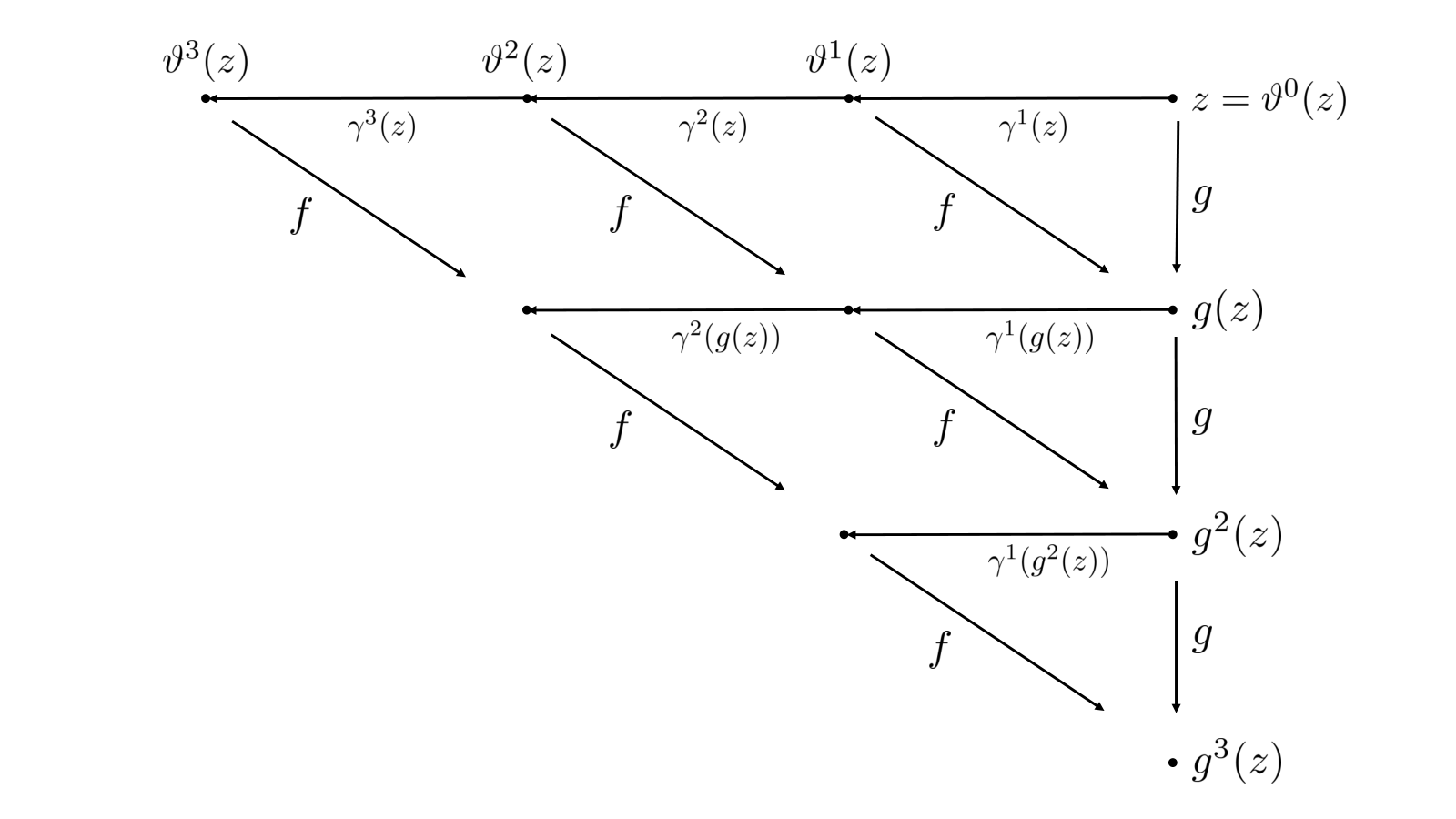
Our goal is to show that, for each , the -length of is bounded independently of , with the bound summable over . This in turn means that the maps form a Cauchy sequence with respect to the metric . Indeed, let denote the -distance between points , i.e. the infimum over the length of all curves connecting and . If , then by construction,
| (9.2) |
We begin by estimating the length of for .
Claim.
There is a constant such that whenever .
Proof.
Suppose that . By choice of ,
In particular, by the definition of , . Since all ramified points of lie in , it is a consequence of Proposition 4.4 that we can estimate from above using the hyperbolic metric on . This is given by
see e.g. [Hay89, Example 9.10]. For , the denominator is bounded below by . So
This completes the proof of the claim. ∎
Claim.
We next claim that
| (9.3) |
Proof.
We prove the claim by induction on ; note that we have just proved (9.3) when . So we can assume that and that the claim holds for . Let . Recall that maps to in one-to-one fashion, and that . By choice of , and since , this means that and lie in the region where agrees with the orbifold metric . Hence we can apply Proposition 4.6, and see that indeed
Now, suppose that and that . Write , where and . Observe that is the pullback of by an inverse branch of . Moreover, . Hence the hypotheses of Proposition 8.1 are satisfied for points in . It follows by Proposition 8.1, together with (9.3), that
where and are the constants from Proposition 8.1. Since these bounds are independent of and summable over , it follows from (9.2) that the maps form a Cauchy sequence with respect to the metric .
By definition of , the density of with respect to the spherical metric on is uniformly bounded from below. In particular, also forms a Cauchy sequence with respect to the spherical metric, and hence converges uniformly to a function in this metric. By Observation 2.4, is docile. ∎
Proof of Corollary 1.4.
Proof of Corollary 1.5.
We use Corollary 1.4. By [BJR12], the Julia set of the disjoint-type function is a Cantor Bouquet. The Julia set can be topologically described as the quotient of by the closed equivalence relation
Since is a bijection, any nontrivial equivalence class is contained in the set of non-escaping points of , which is a subset of the endpoints of the Cantor bouquet. (See [RRRS11, Theorem 5.10].)
Furthermore, preserves the cyclic order of hairs at infinity. (This is easy to see from the construction, but also follows from the fact that, for large as in Theorem 2.1, the restriction of to extends to a quasiconformal homeomorphism of the complex plane by [Rem09].) Hence is indeed a pinched Cantor Bouquet. ∎
Proof of Corollary 1.6.
Proof of Theorem 1.7.
Suppose that is geometrically finite, and that is connected. By assumption is compact, and it is well-known that is simply-connected. Hence, by [RS18, Corollary 8.5], . In particular is strongly geometrically finite.
Let be the semiconjugacy from Corollary 1.4. Suppose, by way of contradiction, that is not injective. Then there are two distinct points such that . Let and be the connected components of containing and respectively. Note that by Corollary 1.4d.
The set of non-escaping points in any component of has zero Hausdorff dimension, see [Rem16, Theorem 2.3], and therefore is totally disconnected. Moreover, is an injection on the escaping set of . Thus is totally disconnected. It is known that the union of two non-separating, closed, connected subsets of the sphere separates the sphere if and only if their intersection is disconnected; see [Mul22]. Hence separates the plane. This is a contradiction, because the Julia set of is nowhere dense, and so the fact that the Fatou set of is connected implies that no closed subset of the Julia set of can separate the plane.
The final claim of the theorem is immediate (again using the fact that the conjugacy preserves the order of hairs). ∎
Proof of Theorem 1.11.
We use the established notions of the symbolic dynamics of exponential maps; see, for example, [RS08] for definitions. As in [RS08], we shall use the parameterisation of exponential maps as
Note that as in (1.1) is conformally conjugate to if and only if . As first proved in [SZ03], the escaping set is an uncountable union of injective curves to infinity, called hairs or dynamic rays. These hairs can be described as the path-connected component of [FRS08, Corollary 4.3]. They are identified by infinite sequences of integers called external addresses, and the lexicographical ordering of addresses corresponds to the vertical ordering of hairs; see [RS08, Section 2]. If are parameters for which the singular values do not belong to the escaping sets, then there is a natural bijection that preserves the external addresses of hairs [Rem06, Theorem 1.1].
If is of disjoint type, then the map is, by construction, the same bijection as in Theorem 2.2, up to a topological conjugacy between the two disjoint-type functions on their Julia sets. (We omit the details.) In particular, is docile if and only if extends continuously to . Let us fix a disjoint-type parameter for the remainder of the proof.
If has an attracting or parabolic orbit, then there is a unique associated intermediate external address ; see [RS08, Section 2] or [Sch03, Lemma 3.3]. If has an attracting orbit, i.e. if is hyperbolic, then this address completely determines the dynamics on the Julia set as follows: Two hairs of land together if and only if their external addresses have the same itinerary with respect to [Rem06, Proposition 9.2]. In particular, determines completely which endpoints of the Cantor bouquet are identified by the extension of .
The proof of [Rem06, Proposition 9.2] uses contraction properties of a suitable hyperbolic metric. Replacing the hyperbolic metric by our metric , and using Proposition 8.1, we see that the same result holds for any exponential map with a parabolic cycle. Now let be such a parabolic parameter. Then by [Sch03, Theorem 3.5], there is a unique hyperbolic component consisting of parameters with . (In [Sch03], the theorem is stated for the family ; see [RS08, Proposition 4.2] for the corresponding statement in the -plane.) By Theorem 1.3 and the above, the bijection of escaping sets extends to a conjugacy . By construction, this conjugacy preserves external addresses, and therefore the vertical order of hairs. This shows that has the property claimed in the statement of Theorem 1.11. Moreover, by [RS08, Corollary 5.5], the component is the unique “child component” of the parameter , and in particular .
To show uniqueness, let be as above, and suppose that and are conjugate via a conjugacy that preserves the vertical order of hairs. Then by [Rem06, Proof of Corollary 8.4], there is such that, for , the map extends to a conjugacy between and on their Julia sets. In particular, the hairs at two given external addresses land together for if and only if they do so for . It follows that and have the same characteristic addresses [RS08, Lemma 3.3 and Theorem 3.4], which in turn implies that [RS08, Lemma 3.10]. In other words, belongs to the hyperbolic component at address . As and correspond to the same parameter in our original parameterisation of the exponential family, the proof of the Theorem is complete. ∎
10. Fatou components and local connectivity of the Julia set
We frequently use the following, which combines parts of Propositions 2.8 and 2.9 of [BFR15].
10.1 Proposition.
Suppose that is an entire function, that is a simply connected domain, and that is a component of . Then exactly one of the following holds.
- (a)
The map is proper, and hence has finite degree.
- (b)
For , with at most one exception, is infinite. Also, either contains an asymptotic curve corresponding to an asymptotic value in , or contains infinitely many critical points. Moreover, if is compact, then infinity is accessible in .
If, in addition, is a singleton, then contains at most one critical point of .
We also use the following, which strengthens other parts of [BFR15, Proposition 2.9].
10.2 Proposition.
Proof.
It is easy to see that, at any finite point, is locally an arc. In particular, if is bounded, then it is a Jordan domain.
Now suppose that is unbounded. Then the boundary of in is locally connected. Indeed, this is true at every finite point by the above, and a continuum cannot fail to be locally connected at only a single point; see [Why42, (12.3) in Chapter I].
Let be a Riemann map from to and let be a Riemann map from to . Then is a finite Blaschke product, say , which extends continuously . By the Carathéodory-Torhorst theorem, and , also extend continuously to . Since is unbounded, there is with . It follows that is an asymptotic value of , as claimed. ∎
A key result of this section is the following.
10.3 Theorem (Immediate basins of geometrically finite maps).
Suppose that is strongly geometrically finite, and that is a periodic Fatou component of , of period . Then the following are equivalent:
- (a)
is a Jordan domain;
- (b)
is locally connected at some finite point of ;
- (c)
is bounded;
- (d)
infinity is not accessible from ;
- (e)
the orbit of contains no asymptotic curves and only finitely many critical points;
- (f)
is a proper map;
- (g)
for at least two distinct choices of , the set is finite.
10.4 Remark.
Note that Theorem 10.3 is similar to [BFR15, Theorem 1.10]. That result has the stronger hypothesis that is hyperbolic, and the stronger conclusion that is, in fact, a quasidisc; in other words, the image of the unit disc under a quasiconformal map of the sphere. This stronger result does not hold in general when contains a parabolic point (even if is an immediate attracting basin).
Proof of Theorem 10.3.
The first parts of the proof are as in the proof of [BFR15, Theorem 1.10], and are included for completeness. That is immediate. It follows from [BFR15, Theorem 2.6] that , and the fact that is immediate. Note that, by assumption, is compact. Suppose that infinity is not accessible in . It follows from Proposition 10.1 that the orbit of contains only finitely many critical points and no asymptotic curves. In other words, . The fact that is also a consequence of Proposition 10.1.
It remains to show that f implies a. As earlier in the paper, let be the smallest iterate of such that all periodic Fatou components of are fixed, and all parabolic points are of multiplier one.
Suppose that is a periodic Fatou component of . If is an immediate attracting basin and , then is uniformly expanding in a neighbourhood of , with respect to the metric . In this case, we can follow the proof of [BFR15, Theorem 1.10], and obtain even that is a quasidisc. If is an immediate attracting basin whose boundary contains a parabolic point, then we may still follow the proof of [BFR15, Theorem 1.10], but replacing uniform expansion with Proposition 8.1. We again obtain that is a Jordan domain (but no longer a quasidisc).
Suppose, then, that is an immediate parabolic basin if , with a parabolic fixed point . Recall that, by assumption, is a proper map. Let be the attracting petal from Proposition 5.2 that is contained in . We may assume for simplicity that is piecewise analytic, and analytic except possibly at . Define . Since contains , each is again a piecewise analytic Jordan curve, mapped as a covering map to .
Now define a homotopy between and in . More precisely, we choose a continuous function
such that:
- (a)
is a homeomorphism;
- (b)
is a homeomorphism;
- (c)
for all ;
- (d)
for and .
Consider the curve , which connects to . Clearly we may assume that is smooth, so that the Euclidean length of is uniformly bounded.
Moreover, for sufficiently close to , we may suppose that is the image of under the branch of that fixes . We have
(Here is the multiplicity of , as before.) It is easy to see that we can let the length of to be of the same order. In summary, the Euclidean length satisfies
and the -length satisfies
| (10.1) |
(Recall that was defined in (7.1).)
We now extend to a map on as follows. For , let be the unique number such that . Since is a covering map, there is a unique continuous extension of to such that
for all .
Continuing inductively, we obtain the desired extension
For and , the curve connects and , and is a pullback of the curve for some .
Since , these lengths are summable, and it follows that the functions converge uniformly in the metric to a continuous function . Since converges to in the Hausdorff metric on the sphere, is surjective. In particular, is bounded and is locally connected. By the maximum principle and Montel’s theorem, is full with , and it follows that is indeed a Jordan curve. ∎
Proof of Theorem 1.8.
Suppose that is strongly geometrically finite. If has an asymptotic value, then, by the definition of a strongly geometrically finite map, this lies in the Fatou set, and so has an unbounded Fatou component. If a Fatou component contains infinitely many critical points, then these must accumulate at infinity and so the component must be unbounded. This completes the proof in one direction.
To prove the other direction, suppose that has no asymptotic values and that each component of contains at most finitely many critical points. It follows from Theorem 10.3 that every periodic Fatou component of is a bounded Jordan domain.
Suppose that is a Fatou component of , and let be the Fatou component of containing . We claim that if is a bounded Jordan domain, then so is . Since, by Proposition 5.3, has no wandering domains, it follows from this claim that all Fatou components of are bounded Jordan domains, completing the proof.
We can now deduce Theorem 1.9. The proof is a generalisation of [BFR15, Theorem 2.5] to strongly geometrically finite maps; see also [Mor99, Theorem 2].
Proof of Theorem 1.9.
Suppose that satisfies the hypotheses of the theorem; that is, is strongly geometrically finite with no asymptotic values, and there is a uniform bound on the number of critical points, counting multiplicity, in each Fatou component. In particular, satisfies the hypotheses of Theorem 1.8, and hence every Fatou component of is a bounded Jordan domain.
It follows by [Why42, Thm. 4.4, Chapter VI], and see also [BFR15, comments after Lemma 2.3], that a compact subset of the sphere is locally connected if and only if the following conditions both hold:
- (a)
the boundary of each complementary component is locally connected;
- (b)
for each there are only finitely many complementary components of spherical diameter greater than .
By the above, the Julia set satisfies a. So it remains to show that b also holds. In other words, we have to show that for each there are only finitely many Fatou components of spherical diameter greater than . By passing to an iterate, we may assume that all periodic Fatou components are invariant; in particular, all parabolic points of are fixed and of multiplier one.
Since has only finitely many attracting or parabolic basins, it is enough to establish b for the connected components of each such basin separately. So suppose that is an immediate attracting or parabolic basin. For each , we choose a set as follows.
- (a)
If , then we choose to be a round disc around whose closure does not contain any postsingular points of , except possibly itself.
- (b)
If , we choose a union of thin repelling petals at , for each repelling direction at , and set . We may choose these sectors small enough that contains no postsingular points other than .
In each case, is a relative neighbourhood of in . Let be such that every point in can be connected to by a curve of -length at most . Consider the collection of connected components of . Each contains exactly one element of . Let be the smallest number such that every point of can be connected to this element by a curve of -length at most ; we call the radius of . Since does not expand the metric , we have , and moreover when .
Claim.
The radius of tends to zero uniformly as .
Proof.
If , then is bounded from below for by choice of . It follows from Proposition 8.1 that
for , showing that the radius tends to zero as desired.
On the other hand, suppose that , and let . If , then there is , independent of , such that all points have . As above, by Proposition 8.1, there is a sequence with such that every connected component of has radius at most , for all and all with .
On the other hand, for each , there is exactly one with , and we have . Since consists of repelling petals, together with , we have . Therefore as .
Now let , and let be minimal such that . Then, on the one hand,
On the other hand, if , then is contained in an element of that does not contain , and therefore
Therefore
Clearly as , as desired. ∎
Claim.
Let denote the connected components of , other than itself. Then the -diameter of tends to zero uniformly as .
Proof.
Since is compact and locally connected, we may choose finitely many points such that the connected components of containing cover . Write . By the claim, there is such that the -diameter of is at most .
If , then we can cover by sets from , where is the degree of . By assumption, this degree is uniformly bounded. Indeed, Since is compact, only a finite number, say, of the Fatou components of intersect . By the Riemann-Hurwitz formula, and by assumption, the degree of on any Fatou component is bounded by . Thus , and therefore . ∎
In particular, the spherical diameter of tends to zero uniformly as . On the other hand, for fixed the different elements of can accumulate only at ; see [BR20, Lemma 2.1]. In other words, for a given , only finitely many contain elements of spherical diameter at least , and for each the number of such elements is finite. The proof of the theorem is complete. ∎
11. Examples
In this final section we give some examples. We begin with the simplest example of a transcendental entire function that is (strongly) geometrically finite but not subhyperbolic.
11.1 Example.
Let . Then is strongly geometrically finite, but not subhyperbolic.
Proof.
We have . Moreover, is a parabolic fixed point of . Since its immediate basin must contain a singular value – or by elementary considerations – we have . Hence , and is strongly geometrically finite, but is not compact and so is not subhyperbolic. It is straightforward to show that is connected. Hence, by Theorem 1.7, is topologically conjugate on its Julia set to any map of the form , for . In particular, as noted earlier, is a Cantor bouquet.∎
Our second example, mentioned in the introduction, shows that the Julia set of the sine function is locally connected.
11.2 Example.
Let . Then is strongly geometrically finite, and is locally connected.
Proof.
Note that . The origin is a parabolic fixed point of , and it is easy to see that both points of lie in the parabolic basin of this point. It follows that , and is strongly geometrically finite. All points on the imaginary axis apart from the origin lie in , and so the whole imaginary axis lies in . Thus the two singular values of lie in different Fatou components. Hence the assumptions of Corollary 1.10 are satisfied, and so is locally connected. ∎


A transcendental entire function is parabolic if , and is finite and contained in . Note that Examples 11.1 and 11.2 are both parabolic, and so covered by the results of [Alh18]. Our next example is a transcendental entire function that is geometrically finite but not parabolic.
11.3 Example.
Let . Then is geometrically finite, but not parabolic, not strongly geometrically finite, and not docile.
Proof.
It can be seen that has one asymptotic value, at the origin, which is fixed and parabolic. It also has one critical value, at , and this is in the parabolic basin. Hence is geometrically finite, but not parabolic since . Since is an asymptotic value, is also not strongly geometrically finite.
Remark.
A similar argument shows that, more generally, a function having a direct asymptotic value in the Julia set cannot be docile.
Our final example is a transcendental entire function which is not parabolic, but which is strongly geometrically finite.
11.4 Example.
For each such that , define the transcendental entire function
For a suitable value of , the function is strongly geometrically finite, but neither subhyperbolic nor parabolic. The Julia set is locally connected.
Proof.
Note that has no asymptotic values, and
Also, the origin is a parabolic fixed point of . We choose such that
in fact, it can be seen that there is a unique such , with . It follows that one critical value of is at . Since , this critical values lies in the Julia set. It can be checked that the other critical value lies in the parabolic basin, and hence is geometrically finite. As is obtained from up to pre-and post-composition with affine functions, it has no asymptotic values, and all critical points are simple. Therefore has bounded criticality, and is strongly geometrically finite. By Corollary 1.10, the Julia set is locally connected.
∎
Acknowledgments
We are grateful to David Martí Pete, Leticia Pardo Simón and James Waterman for helpful discussions and feedback concerning this paper.
References
- [Alh18] Mashael Alhamed, Dynamics of parabolic transcendental entire functions, Ph.D. thesis, University of Liverpool, 2018.
- [AO93] Jan M. Aarts and Lex G. Oversteegen, The geometry of Julia sets, Trans. Amer. Math. Soc. 338 (1993), no. 2, 897–918.
- [Bea91] A. F. Beardon, Iteration of rational functions, Springer, 1991 (English).
- [Ber93] W. Bergweiler, Iteration of meromorphic functions, Bull. Amer. Math. Soc. (N.S.) 29 (1993), no. 2, 151–188.
- [BFR15] Walter Bergweiler, Núria Fagella, and Lasse Rempe-Gillen, Hyperbolic entire functions with bounded Fatou components, Comment. Math. Helv. 90 (2015), no. 4, 799–829.
- [BJR12] Krzysztof Barański, Xavier Jarque, and Lasse Rempe, Brushing the hairs of transcendental entire functions, Topology Appl. 159 (2012), no. 8, 2102–2114.
- [BK07] Krzysztof Barański and Bogusława Karpińska, Coding trees and boundaries of attracting basins for some entire maps, Nonlinearity 20 (2007), no. 2, 391–415.
- [BP78] A. F. Beardon and Ch. Pommerenke, The Poincaré metric of plane domains, J. London Math. Soc. (2) 18 (1978), no. 3, 475–483.
- [BR20] Anna Miriam Benini and Lasse Rempe, A landing theorem for entire functions with bounded post-singular sets, Geom. Funct. Anal. 30 (2020), no. 6, 1465–1530.
- [Car13] C. Carathéodory, Über die Begrenzung einfach zusammenhängender Gebiete, Math. Ann. 73 (1913), no. 3, 323–370.
- [CG93] Lennart Carleson and Theodore W. Gamelin, Complex dynamics, Universitext: Tracts in Mathematics, Springer-Verlag, New York, 1993.
- [CT18] Guizhen Cui and Lei Tan, Hyperbolic-parabolic deformations of rational maps, Sci. China Math. 61 (2018), no. 12, 2157–2220.
- [DK84] Robert L. Devaney and Michał Krych, Dynamics of , Ergodic Theory Dynam. Systems 4 (1984), no. 1, 35–52.
- [EL92] A. E. Eremenko and M. Yu. Lyubich, Dynamical properties of some classes of entire functions, Ann. Inst. Fourier (Grenoble) 42 (1992), no. 4, 989–1020.
- [FRS08] Markus Förster, Lasse Rempe, and Dierk Schleicher, Classification of escaping exponential maps, Proc. Amer. Math. Soc. 136 (2008), no. 2, 651–663.
- [Ha98] Peter Haïssinsky, Chirurgie parabolique, C. R. Acad. Sci. Paris Sér. I Math. 327 (1998), no. 2, 195–198.
- [Ha00] by same author, Déformation -équivalente de polynômes géometriquement finis, Fund. Math. 163 (2000), no. 2, 131–141.
- [Ha02] by same author, Pincement de polynômes, Comment. Math. Helv. 77 (2002), no. 1, 1–23.
- [Hay89] W. K. Hayman, Subharmonic functions. Vol. 2, London Mathematical Society Monographs, vol. 20, Academic Press Inc. [Harcourt Brace Jovanovich Publishers], London, 1989.
- [Jar11] Xavier Jarque, On the connectivity of the escaping set for complex exponential Misiurewicz parameters, Proc. Amer. Math. Soc. 139 (2011), no. 6, 2057–2065.
- [Kah98] Jeremy Kahn, Holomorphic removability of Julia sets, 1998.
- [Kaw03] Tomoki Kawahira, Semiconjugacies between the Julia sets of geometrically finite rational maps, Ergodic Theory Dynam. Systems 23 (2003), no. 4, 1125–1152.
- [Kaw06] by same author, Semiconjugacies between the Julia sets of geometrically finite rational maps. II, Dynamics on the Riemann sphere, Eur. Math. Soc., Zürich, 2006, pp. 131–138.
- [McM94] Curtis T. McMullen, Complex dynamics and renormalization, Annals of Mathematics Studies, vol. 135, Princeton University Press, Princeton, NJ, 1994.
- [McM00] by same author, Hausdorff dimension and conformal dynamics. II. Geometrically finite rational maps, Comment. Math. Helv. 75 (2000), no. 4, 535–593.
- [Mih09] Helena Mihaljević-Brandt, Topological dynamics of transcendental entire functions, Ph.D. thesis, University of Liverpool, 2009.
- [Mih10] by same author, A landing theorem for dynamic rays of geometrically finite entire functions, J. Lond. Math. Soc. (2) 81 (2010), no. 3, 696–714.
- [Mih12] by same author, Semiconjugacies, pinched Cantor bouquets and hyperbolic orbifolds, Trans. Amer. Math. Soc. 364 (2012), no. 8, 4053–4083.
- [Mil00] John Milnor, Local connectivity of Julia sets: expository lectures, The Mandelbrot set, theme and variations, London Math. Soc. Lecture Note Ser., vol. 274, Cambridge Univ. Press, Cambridge, 2000, pp. 67–116.
- [Mil06] by same author, Dynamics in one complex variable, third ed., Annals of Mathematics Studies, vol. 160, Princeton University Press, Princeton, NJ, 2006.
- [Mor99] Shunsuke Morosawa, Local connectedness of Julia sets for transcendental entire functions, Nonlinear analysis and convex analysis (Niigata, 1998), World Sci. Publ., River Edge, NJ, 1999, pp. 266–273.
- [Mul22] Anna M. Mullikin, Certain theorems relating to plane connected point sets, Trans. Amer. Math. Soc. 24 (1922), no. 2, 144–162.
- [Osb13] J. W. Osborne, Spiders’ webs and locally connected Julia sets of transcendental entire functions, Ergodic Theory Dynam. Systems 33 (2013), no. 4, 1146–1161.
- [Par19] Leticia Pardo-Simón, Splitting hairs with transcendental entire functions, Preprint, arXiv:1905.03778v1, 2019.
- [Pom92] Ch. Pommerenke, Boundary behaviour of conformal maps, Grundlehren der Mathematischen Wissenschaften [Fundamental Principles of Mathematical Sciences], vol. 299, Springer-Verlag, Berlin, 1992.
- [Rem06] Lasse Rempe, Topological dynamics of exponential maps on their escaping sets, Ergodic Theory Dynam. Systems 26 (2006), no. 6, 1939–1975.
- [Rem07] by same author, On a question of Eremenko concerning escaping components of entire functions, Bull. Lond. Math. Soc. 39 (2007), no. 4, 661–666.
- [Rem09] by same author, Rigidity of escaping dynamics for transcendental entire functions, Acta Math. 203 (2009), no. 2, 235–267.
- [Rem16] by same author, Arc-like continua, Julia sets of entire functions, and Eremenko’s conjecture, Preprint, arXiv:1610.06278v2, 2016.
- [RRRS11] Günter Rottenfusser, Johannes Rückert, Lasse Rempe, and Dierk Schleicher, Dynamic rays of bounded-type entire functions, Ann. of Math. (2) 173 (2011), no. 1, 77–125.
- [RS08] Lasse Rempe and Dierk Schleicher, Combinatorics of bifurcations in exponential parameter space, Transcendental dynamics and complex analysis, London Math. Soc. Lecture Note Ser., vol. 348, Cambridge Univ. Press, Cambridge, 2008, pp. 317–370.
- [RS12] P. J. Rippon and G. M. Stallard, Fast escaping points of entire functions, Proc. Lond. Math. Soc. (3) 105 (2012), no. 4, 787–820.
- [RS17] Lasse Rempe-Gillen and Dave Sixsmith, Hyperbolic entire functions and the Eremenko-Lyubich class: class or not class ?, Math. Z. 286 (2017), no. 3-4, 783–800.
- [RS18] by same author, On connected preimages of simply-connected domains under entire functions, To appear in Geom. Funct. Anal., arXiv:1801.06359v1, 2018.
- [RS19] P. J. Rippon and G. M. Stallard, Eremenko points and the structure of the escaping set, To appear in Trans. Amer. Math. Soc., arXiv:1703.11001v1, 2019.
- [Sch03] Dierk Schleicher, Attracting dynamics of exponential maps, Ann. Acad. Sci. Fenn. Math. 28 (2003), no. 1, 3–34.
- [Sch10] by same author, Dynamics of entire functions, Holomorphic dynamical systems, Lecture Notes in Math., vol. 1998, Springer, Berlin, 2010, pp. 295–339.
- [Six18] David J. Sixsmith, Dynamics in the Eremenko-Lyubich class, Conform. Geom. Dyn. 22 (2018), 185–224.
- [SZ03] Dierk Schleicher and Johannes Zimmer, Escaping points of exponential maps, J. London Math. Soc. (2) 67 (2003), no. 2, 380–400.
- [Thu79] W. P. Thurston, Geometry and topology of three-manifolds, Princeton Lecture Notes, 1979.
- [Thu84] by same author, On the combinatorics and dynamics of iterated rational maps, Preprint, 1984.
- [Tor21] Marie Torhorst, Über den Rand der einfach zusammenhängenden ebenen Gebiete, Math. Z. 9 (1921), no. 1-2, 44–65.
- [TY96] Lei Tan and Yongcheng Yin, Local connectivity of the Julia set for geometrically finite rational maps, Sci. China Ser. A 39 (1996), no. 1, 39–47.
- [Why42] Gordon Thomas Whyburn, Analytic Topology, American Mathematical Society Colloquium Publications, v. 28, American Mathematical Society, New York, 1942.
- [Wor18] Stephen Worsley, The topology of postsingularly finite exponential maps, Ph.D. thesis, University of Liverpool, 2018.