Dust and gas content of high-redshift galaxies hosting obscured AGN in the CDF-S
Abstract
Context. Obscured active galactic nuclei (AGN) represent a significant fraction of the entire AGN population, especially at high redshift (70% at z=3–5). They are often characterized by the presence of large gas and dust reservoirs that are thought to sustain and possibly obscure vigorous star formation processes that make these objects shine at far-IR and submillimeter wavelengths. Studying the physical properties of obscured AGN and their host galaxies is crucial to shedding light on the early stages of a massive system lifetime.
Aims. We aim to investigate the contribution of the interstellar medium (ISM) to the obscuration of quasars in a sample of distant highly star forming galaxies and to unveil their morphological and kinematics properties.
Methods. We exploit Atacama Large Millimeter/submillimeter Array (ALMA) Cycle 4 observations of the continuum (2.1mm) and high-J CO emission of a sample of six X-ray selected, far-IR detected galaxies hosting an obscured AGN at in the 7 Ms Chandra Deep Field-South (CDF-S). We measured the masses and sizes of the dust and molecular gas by fitting the images, visibilities, and spectra, and we derived the gas density and column density on the basis of a uniform sphere geometry. Finally, we compared the measured column densities with those derived from the Chandra X-ray spectra.
Results. We detected both the continuum and line emission for three sources for which we measured both the flux density and size. For the undetected sources, we derived an upper limit on the flux density from the root mean square (rms) of the images. We found that the detected galaxies are rich in gas and dust (molecular gas mass in the range ¡ - for and up to for , and dust mass ¡ - ) and generally compact (gas major axis 2.1-3.0 kpc, dust major axis 1.4-2.7 kpc). The column densities associated with the ISM are on the order of , which is comparable with those derived from the X-ray spectra. For the detected sources we also derived dynamical masses in the range - .
Conclusions. We conclude that the ISM of high redshift galaxies can substantially contribute to nuclear obscuration up to the Compton-thick () regime. In addition, we found that all the detected sources show a velocity gradient reminding one rotating system, even though two of them show peculiar features in their morphology that can be associated with a chaotic, possibly merging, structure.
Key Words.
galaxies: active – galaxies: evolution – galaxies: high-redshift – submillimeter: galaxies – ISM: structure –ISM: kinematics and dynamics1 Introduction
Active galactic nuclei (AGN) are characterized by accretion onto super massive black holes (SMBHs) which powers their emission over twenty decades in frequency. Almost all massive galaxies are thought to host a central SMBH which has passed (and possibly will pass) through active accretion phases during their life. Indeed, there is increasing evidence for a close connection between the star formation rate (SFR) and BH accretion history, suggesting a coevolution of the BH and its host galaxy; in particular, a crucial phase of such evolution occurs at = 2 – 3, when both the SFR and BH accretion reach their maximum over cosmic time (Gruppioni et al. 2013; Madau & Dickinson 2014, e.g.,). The unified models postulate that nuclear absorption is due to a parsec-scale medium distributed in a toroidal geometry around the central engine (Urry & Padovani 1995). Nevertheless, the large amount of gas required to sustain the vigorous star formation (SF) of these objects during the epoch of their activity peak suggests that the UV and X-ray emission from the very central region of the galaxy can be obscured by the interstellar medium (ISM) located up to kiloparsec-scale in the host galaxy. In addition, the high-z ( ) heavily obscured (column density ) AGN fraction is estimated to be 70% (Vito et al. 2018), which is significantly higher than in the local Universe (Burlon et al. 2011, intrinsic distribution 43% for the same column density,). This suggests an evolution of the luminous obscured AGN fraction, which may be driven by the larger gas content observed in high-z galaxies (Carilli & Walter 2013, e.g.,).
Several concurring physical processes are responsible for the formation of galaxies and the build-up of their mass: for example, major mergers between gas–rich galaxies (Hopkins & Beacom 2006, e.g.,), mass inflows from the cosmic web (Dekel et al. 2009; Bournaud et al. 2011), or fast collapse in early halos during which most of the mass of the system is accreted (Lapi et al. 2014; Lapi et al. 2018, e.g.,); in all these scenarios the central regions are fueled with gas, triggering SF and BH accretion. Recent data from ALMA, Institut de radioastronomie millimétrique (IRAM) and Herschel indicate short gas depletion timescales (Genzel et al. 2015; Tacconi et al. 2018, some yr, see). The submillimeter galaxies (SMGs, defined as submilllimeter objects having flux densities 1 mJy at 850 m, Carilli & Walter 2013 Carilli & Walter 2013; see also Circosta et al. 2019 Circosta et al. 2019 and references therein) are often indicated as those objects that trace the brief phase at the peak of SFR in the galaxy evolution. They are usually detected at median redshift 2-3 (Simpson et al. 2014), and are characterized by extremely dense ISM, showing molecular masses up to and dust masses up to few distributed on kiloparsec scales (Swinbank et al. 2014; Barro et al. 2014; Ikarashi et al. 2015; Massardi et al. 2018; Lapi et al. 2018). The estimated SFR of these objects is (Blain et al. 2002; Swinbank et al. 2014). These properties make SMGs the best targets to investigate the contribution of the host galaxy in obscuring the AGN. Moreover, many observations revealed that these sources have morphologies showing complex gas motions and that the star–forming gas can lie in compact, rotating disk structures (Tacconi et al. 2008; Hodge et al. 2012; Ivison et al. 2013; De Breuck et al. 2014). Given their high gas and dust density and small size, SMGs are also considered among the best candidates as progenitors of compact quiescent galaxies (Cimatti et al. 2008, cQGs), a class of quiescent galaxies that are considerably smaller and denser than local galaxy counterparts of similar mass, showing stellar half–light radii of kpc and typical stellar masses of (Cassata et al. 2011).
Estimating the column density associated with the ISM of the host galaxy requires a multiwavelength approach exploiting data from the X-rays to the submillimeter: on the one hand, the X-rays directly probe the innermost region of the sources and can be used to evaluate the line of sight absorption to the central engine emission. On the other hand, the mm band is crucial to estimate the ISM properties such as the mass and geometrical distribution of the gas and dust components. In particular, measurement of the gas mass, dominated by the molecular component at 2 (Carilli & Walter 2013), can be achieved with different methods: the most common exploits the low-J transition of CO as a tracer of the total molecular gas mass. An alternative method exploits the monochromatic continuum dust luminosity at 850 m (): Scoville et al. 2016 showed an empirical relation between and the CO(1–0) emission line luminosity – valid for local ultraluminous infrared galaxies (ULIRGs, ), z2 SMGs and local star-forming galaxies – from which they derived a direct relation between and the molecular gas mass, assuming a Galactic CO-to- conversion factor. Once the gas mass and size are measured through high resolution observation, the gas column density can be derived assuming a geometrical configuration.
Gilli et al. 2014 found that the column densities derived from the X-ray spectral analysis and the ISM mass are comparable for a SMG at = 4.755 hosting a heavily obscured AGN (XID 539, included in our sample, Table 1). This source is also included in the sample studied by Circosta et al. 2019, who performed an in-depth analysis on seven X-ray selected, far infrared (FIR) detected AGN with spectroscopic redshift ¿ 2.5 in the 7 Ms Chandra Deep Field-South (CDF-S), in order to assess whether and to what extent the host ISM contributes to the AGN obscuration. They performed X-ray spectral fitting to derive the column density responsible for the central obscuration, assuming different spectral models. Then they exploited the available UV-to-FIR photometric data to derive the 850 m flux from spectral energy distribution (SED) fitting, and they converted it into gas mass assuming the Scoville et al. 2016 empirical relation and the CO-to- conversion factor = 0.8 . On the basis of a simple assumption of spherical gas distribution with uniform density, they derived column densities of the host ISM that are comparable with those extracted from the X-ray fitting, and concluded that the ISM likely plays a significant role in the obscuration.
In this work we analyze for the first time the millimetric emission of the high-J CO emission and the dust continuum of six heavily obscured AGN (X-ray column densities ¿ ) in the CDF-S at spectroscopic ¿ 2.5, included in the sample of Circosta et al. 2019 and observed with ALMA. In Sec. 2 we illustrate the criteria adopted to select the targets and summarize the sample properties. In Sec. 3 we describe the ALMA observations and the data reduction process. In Sec. 4 we perform the imaging and obtain the flux density, the angular size and line shape of the sources from both the spectrum and visibility fitting. We exploit these quantities in Sec. 5 to derive the mass and physical size of both the dust and molecular gas content. As for the gas mass, we explore several cases with different assumptions on the involved conversion factors, to address the large uncertainties in deriving such mass from both high-J CO transitions and dust long-wavelength emission. Then we derive the column densities for a simple spherical geometry and compare them with those measured from the X-ray spectra by Circosta et al. 2019. We also calculate the dust mass in the optically–thin regime and the dynamical mass of the two sources for which the rotating disk model has been tested. Finally, in Sec. 6 we summarize and discuss the results and future perspectives.
Throughout the paper we adopt a standard CDM cosmology: , , (Bennett et al. 2014). As for the reported velocities we adopt the radio definition v = , where and are the rest and observed frequency, respectively, in a Barycentric (i.e., referred to the Sun and Earth center of mass) rest-frame.
2 Sample selection
The Chandra Deep Field South (Luo et al. 2017, CDF-S, ,) provides the best X-ray spectral information currently available for distant AGN, thanks to its 7-Ms exposure time (Luo et al. 2017, the average flux limit within 1 arcmin from the center of the field is ,). In addition, this field features an exceptional multiwavelength coverage that allows the characterization of the overall SED of most X-ray sources with extraordinary accuracy. In particular, deep IR observations have been carried out with the Hubble Space Telescope (HST), Herschel and Spitzer observatories. Moreover, many observations in the submillimeter band were taken with instruments such as the Submillimeter Common-User Bolometer Array (SCUBA) on the James Clerk Maxwell Telescope and the Large Apex BOlometer CAmera (LABOCA) on the Apex Telescope. The central area of the CDF–S (about 1/3 of the whole field) is covered by the Great Observatories Origins Deep Survey (Giavalisco et al. 2004, GOODS–S,), in which the Cosmic Near–IR Deep Extragalactic Legacy Survey (Grogin et al. 2011, CANDELS,), a powerful imaging survey of the distant universe, has been carried out with HST. CANDELS consists of two different areas and depth portions, the deeper and smaller CANDELS/Deep and the shallower and more extended CANDELS/Wide. The CDF-S was also observed by the Galaxy Evolution from Morphology and SEDs (Rix et al. 2004, GEMS,) survey, a large-area (800 ) two-color (F606W and F850LP) imaging survey with the Advanced Camera for Surveys (ACS) on the HST.
In order to select our sources, we combined the sample from Vito et al. 2013, consisting in 34 X-ray selected AGN at in the 4-Ms CDF-S with eight heavily obscured quasars (QSOs) in the redshift range 1.1–3.7, X-ray selected in the 1–Ms CDF-S exposure and observed at 850 m with SCUBA (Rigopoulou et al. 2009). To select our targets from this combined sample we applied the following criteria. Firstly we required a secure (errors ¡ 300 km/s) spectroscopic redshift ¿ 2.5 as given by Luo et al. 2017, in order to avoid the large uncertainties related to the photometric redshift that would propagated in the derived fundamental quantities for our study (such as the intrinsic luminosity) and properly select the CO emission lines to target in the ALMA observations. The redshift threshold at = 2.5 was chosen as a compromise between a sufficiently large gas content in the galaxies (expected to be larger at high-z, such that the host galaxy obscuration might be important) and the size of the sample. Secondly we required at least one ¿ 3 detection at ¿ 100 m, in order to characterize the FIR-SED and maximize the detection probability with ALMA. Finally we included among the sample only the sources with gas column density (derived from the X-ray spectral fitting), in order to consider only heavily obscured objects and trace the evolutionary stage in which the AGN is still deeply buried and the SF is high.
This selection returns six targets spanning the redshift range 2.5 – 4.8. This sample includes six of the seven sources studied by Circosta et al. 2019, who adopted our same selection criteria except for the requirement of heavy obscuration. As pointed out by those authors, the fact that the FIR detection criterion is sufficient to select only obscured AGN indicates a connection between the SF-heated dust in the ISM that is responsible for the FIR to (sub)millimeter emission and the nuclear absorption. Despite the small number of sources (owing to the stringent selection criteria), this sample represents a complete and unique collection of objects: they are characterized by a relatively high number of photons (from 260 to 2000 in the 7–Ms exposure) in the observed 0.5-7 keV band which allows an accurate estimate of the X-ray absorption and by good IR coverage. The IDs, coordinates and redshift are reported in Table 1. Throughout the paper we adopt for our targets the Luo et al. 2017 X-ray Identification numbers (XIDs).
| XID | XID | CID | RA | DEC | |
|---|---|---|---|---|---|
| (1) | (2) | (3) | (4) | (5) | (6) |
| 34 | 42 | 326 a aa a aa This source is not included in CANDELS, thus the ID from GEMS (Häussler et al. 2007) is reported. | 2.940 b bb b bb Using the CIV, HeII and NV lines in the UV–spectrum we derive a better estimate of (See Sec. 4). | ||
| 262 | 337 | 5479 | 3.660 | ||
| 403 | 539 | 273 | 4.755 | ||
| 412 | 551 | 6294 | 3.700 | ||
| 490 | 666 | 9834 | 2.578 | ||
| 546 | 746 | 10578 | 3.064 |
The selected objects are all included in CANDELS/Deep area, except for XID 539 that lies in CANDELS/Wide and XID 42 that is outside CANDELS, but it is included in the GEMS catalog, in the multiwavelength survey by Yale–Chile (MUSYC) catalog (Gawiser & MUSYC Collaboration 2003, consisting of deep optical medium-band and broadband optical and near–IR imaging of the CFDF–S,), and it has been also observed in the band by HST wide field camera 3 (WFC3) (Chen et al. 2015).
Circosta et al. 2019 (Circosta et al. 2019, see Table 4) derived their basic quantities (such as SFR, IR luminosity and stellar mass) by the SED decomposition technique, finding that the targets are massive (stellar mass ) and very luminous (infrared luminosity in the 8-1000 m band ) galaxies. They derived SFRs of (except for XID 42 which has ), which places all sources within 1 from the best fit main sequence relation found by Schreiber et al. 2015 at the corresponding redshift (2 for XID 337 which is below the main sequence). Three of them are well known heavily obscured AGN: XID 337 was firstly detected in the early 1-Ms CDF-S exposure and classified as a type II QSO object in the spectroscopic follow–up (Szokoly et al. 2004). This result was later confirmed by Mainieri et al. 2005 who also reported a submillimeter detection at 850 m using SCUBA. Exploiting high resolution (0.2”) ALMA observations, Circosta et al. 2019 found that the single object associated with XID 337 in the Spitzer/MIPS, Herschel and SCUBA maps is actually a blend of two sources, whose emission is dominated by a bright QSO at 3.5” separation; thus, the Mid-IR/Far-IR photometric datapoints of XID 337 were converted into upper limits. XID 551 was the first type II AGN ever detected in the CDF-S 1-Ms exposure at z¿3 (Norman et al. 2002), for which Comastri et al. 2011 found a large column density () performing an X-ray spectrum analysis using 3.3–Ms XMM-Newton survey data. XID 539 (Hodge et al. 2013, ALESS73.1,) is the most distant Compton-thick AGN known (Gilli et al. 2011), and one of the widely studied sources in the CDF-S (Coppin et al. 2010; Nagao et al. 2012; De Breuck et al. 2014). In particular, Gilli et al. 2014 have performed an in–depth analysis through an observation of the continuum at 1.3 mm, combining it with continuum observations from ALESS and from Nagao et al. 2012. They built a full SED including Herschel data and obtained dust temperature and size and the SFR. XID 666 (BzK 4892) is a Compton-thick QSO studied by Feruglio et al. 2011; Del Moro et al. 2016; Perna et al. 2018. XID 42 (ALESS57.1) has been recently studied by Calistro Rivera et al. 2018 an by Rybak et al. 2019, who resolved the CO(3-2) and [C ii] emission, respectively. XID 746 is the less studied objects, despite being known as Type II QSO since the first 1–Ms exposure in the CDF-S (Szokoly et al. 2004).
3 Observations
ALMA dramatically improved our knowledge of SMGs, providing us with extremely deep and high-resolution images and spectra, which can be used to probe the dust mass and temperature of these objects, their star formation activity, and their gas mass.
We performed ALMA observations (Cycle 4, Band 4, ID: 2015.1.01205.S, PI: R. Gilli) of the continuum at 2.1 mm (142.78 GHz) and of one high-J CO transition for each of the targets, reported in Table 2 along with their rest- and observed-frame frequencies. The requested sensitivity was Jy/beam for the line emission (considering a line width of 200 km/s) that corresponds to 20 Jy/beam for the continuum.
The imaging parameters and procedure used to achieve the reported resolution and sensitivity are described in details in Sec. 4.1 for the CO observation and in Sec. 4.3 for the continuum.
The rms is the defined as the mean rms measured on the images in four regions located at ” from the sources.
| XID | CO line | ||||||
|---|---|---|---|---|---|---|---|
| (1) | (2) | (3) | (4) | (5) | (6) | (7) | (8) |
| 42 | (5-4) | 576.27 | 146.13 | 0.280 0.246 | 0.335 0.310 | 347 | 19 |
| 337 | (6-5) | 691.47 | 148.38 | 0.573 0.532 | 0.592 0.542 | 274 | 26 |
| 539 | (7-6) | 806.65 | 140.16 | 0.302 0.283 | 0.317 0.301 | 195 | 21 |
| 551 | (6-5) | 691.47 | 147.12 | 0.572 0.531 | 0.591 0.541 | 261 | 26 |
| 666 | (4-3) | 461.04 | 128.85 | 0.326 0.306 | 0.302 0.298 | 312/273 a aa a aa The two values correspond to the blue- and red-shifted peaks, respectively (see Fig. 2). | 20 |
| 746 | (5-4) | 576.27 | 141.80 | 0.571 0.524 | 0.565 0.540 | 280 | 23 |
The observations were split in two blocks, each containing three targets: the GHz spectral windows (spws) cover the range 126.56-130.33 GHz and 138.56-142.33 GHz to observe XID 666, XID 746 and XID 539, and the range 133.07-136.93 GHz and 145.17-148.93 GHz for XID 42, XID 337 and XID 551. Each spw is sampled in 240 channels of 7.812 MHz width corresponding, at the median frequency of the spws, to 17.5 km/s in velocity for the first block and to 16.6 km/s for the second one. The project was accepted in C priority and was only partially observed at the end of the Cycle 4. In particular, the first block was observed on the September 2016 for about 88 min, and the second block for about 46 min on the September 2016. QSO J0334-4008 was used to calibrate the flux and bandpass, while the QSO J0348-2749 served as phase calibrator33 3 https://almascience.eso.org/alma-data/calibrator-catalogue.
Three out of six sources (namely XID 42, XID 539 and XID 666) were detected in both the line and continuum emission. Concerning the undetected sources, two of them (XID 337 and XID 551) were observed for half of the time needed to achieve the requested sensitivity, while XID 746 is included in the execution block that was observed twice and reached the requested sensitivity.
We performed data-reduction using the ALMA calibration pipeline in CASA version 4.7.0-1. The pipeline procedure automatically flags bad data and performs the calibration; it also produces several diagnostic plots that are useful to identify possible calibration failures and discern additional needed flags. After the inspection of both the diagnostic plots and calibrated data, the calibration resulted to be satisfactory.
4 Data analysis
We performed a standard imaging of the sources by using the clean task of CASA in “velocity” mode for the line emission and “mfs” mode for the continuum. The imaging parameters were chosen as best trade–off between sensitivity and angular resolution (see Sec. 4.1 and Sec. 4.3 for details, Table 2 for the resolution and sensitivity of each observation).

4.1 CO–line imaging
Since the line is not clearly visible from the visibility amplitude–frequency plane, we cannot unambiguously assess the channels containing it, thus we cannot a priori exclude them when we image the continuum emission. Thus we decided to image separately the spw containing the line and the other spws for the continuum, in order to avoid any possible contamination. To image the continuum-subtracted line we preliminarly ran the uvcontsub task, that performs a polynomial fitting of the continuum level and then subtracts it from the data. We fit the continuum using only the spws that do not contain the line, and subtract the resulting fit from the spw in which the line is expected to be. For XID 337, XID 551, and XID 746 it was not possible to determine unambiguously a channel in which the brightness at the source position was significantly above the noise level. For these sources no detection was obtained even applying natural weighting, tapering (0.45”) and a large channel width (120 km/s) to improve the chance of achieving a significant detection. For XID 42, XID 539 and XID 666 imaging we used a robust weighting equal to 0.5, 1, 1, and a channel width of 40, 120 and 40 km/s, respectively. We clearly identified the channels corresponding to the peak of the emission, whose images are reported in the top row of Fig. 1. We detect XID 42, XID 539 and XID 666 with a signal-to-noise ratio (S/N) equal to 6.2, 4.7 and 4.0/4.9, respectively. The S/N is defined as the ratio between the value of the brightest pixel and the root mean square (rms) derived averaging the rms measured in four regions placed at 10” from any source. Since for XID 666 we detected a double peaked line, the two values refer to the blue- and red-shifted peaks. As a confirmation of the detection, we note the central position of the peak in the images (offset with respect to expected source positions ¡ 0.5”, beam sizes in Table 2) and the line feature in the spectra visible in Fig. 2.
We note that only for XID 539 the velocity of the peak channel (reported on the image) is consistent with zero, being the channel central velocity 111.6 km/s and its width is 120 km/s. XID 666 has two peaks shifted respectively by 200 km/s and 150 km/s centered on the rest-frame velocity. This double-peaked line, also clearly visible from the spectrum (Fig. 2), is interpreted as a signature of a rotating structure. This interpretation is also supported by the velocity map (Fig. 3) that shows a continuous gradient along one direction. However, in Sec. 5.5 we briefly explore the possibility that this source is actually a blend of two nonresolved, merging system. The spectroscopic redshift of XID 42 (z = 2.940) was derived by Szokoly et al. 2004 from the FOcal Reducer and low dispersion Spectrograph (FORS) of the Very Large Telescope (VLT). Re-analyzing the same spectrum using the high excitation lines CIV and NV, and the recombination line HeII (that is a robust redshift estimator) we found a better estimate = 2.9369 0.0003, assumed as the rest–frame hereafter (against the value z=2.939 obtained using the Ly- line, which is known to be challenging as exact redshift estimator due to the resonant scattering). From the CO(5–4) line we derived a redshift = 2.94355 0.00001, which is shifted by 500 km/s with respect to the rest–frame velocity. We note that Calistro Rivera et al. 2018 derived a redshift = 2.943 0.002 from the CO(3–2) line, which is compatible within 3 with that derived both from the optical spectrum and from the CO(5–4) transition. This redshift is also consistent with the [C ii] line detected by Rybak et al. 2019. The rest frequency displacement between the CO and [C ii] lines and the UV emission lines could be explained as a difference in radial velocity. Such as spectral displacements have been often reported in the literature (Pentericci et al. 2016; Matthee et al. 2017; Carniani et al. 2018), and interpreted as a consequence of the clumpy structure of high-z galaxies, in which the different components move with respect to each other. High excitation UV-rest-frame lines and the CO (and [C ii]) lines indeed trace different gas phases and may arise from different regions.
4.2 Moments
By using the immoments task we computed the moments 0, 1, 2 for the detected sources, defined as the frequency-integrated flux, the velocity field and the velocity dispersion, respectively. We performed a Gaussian fitting of the line spectrum and derived their central velocity (with respect to the rest-frame velocity at the given redshift) and Full Width at Half Maximum (FWHM); to calculate the moments we considered a velocity range given by , in order to include few channels aside the line and avoid the loss of signal from its wings. For XID 666, to calculate the moments of the entire source, we consider the channels spanning the velocity range from of the blue component to of the red one. In Fig. 2 we show the spectra of the sources and their fits.

We fit the lines of XID 42 and XID 539 with a single Gaussian component, since there are not evident double-peaked features in their spectra. As for XID 666, we fit two Gaussian components on the whole source region (blue ellipse in Fig. 1). Since the two spectral peaks of XID 666 are quite close and likely contaminated by each other, we additionally performed fitting with a single Gaussian component on the spectra of the two spatially separated regions corresponding to the peaks, in order to estimate such contamination and derive the most accurate line width. Both the line width and central velocity of the single blue and red shifted components are fully consistent (within ) with those derived from the spectrum over the entire source region. In the following, we use the line width and central velocity derived from the two Gaussian components fit on the whole region. The fit results are reported in Table 3. We note that the brightness of the peak is not used in any of the following considerations and derived physical quantities.
| XID | FWHM | ||
|---|---|---|---|
| [mJy/beam] | [km/s] | [km/s] | |
| 42 | |||
| 539 | |||
We extracted the moments using as a threshold a value of calculated by the measured rms on the image. Moments are reported in Fig. 3.

4.3 Dust continuum imaging
For each source we imaged all the spws but those containing the CO line. As for the line imaging, for XID 337, XID 551, and XID 746 we apply natural weighting and a 0.45” tapering, without achieving a significant detection. We detected the continuum emission for XID 42, XID 539 and XID 666 with a S/N equal to 6.8, 12.8 and 7.0, respectively, using a robust weighting equal to 1 for all of them. We show the continuum images of the detected sources in the bottom row of Fig. 1.
4.4 Visibility fitting
Since the reconstructed images depend on the deconvolution algorithm and its input values, they do not provide a unique and direct representation of the data but rather a nonlinear mapping from the Fourier domain into the sky plane. Hence, we firstly perform an image fitting with the sole purpose of using the obtained values as starting input parameters to perform the fits directly on the visibilities, which are unaffected by the reconstruction algorithm and pixel correlation as images are. In addition, if the sources are not or barely spatially resolved in the images, the visibility fitting provides an estimate of their angular size even on scales smaller than the synthesized beam.
As for the image fitting, to derive the information about the dust component, we fit the continuum image, while for the gas we fit the moment 0 of the CO-line since it represents the total integrated emission. We performed the fitting using the task imfit, which relies on the algorithm developed by Condon 1997 using as a model a spatial elliptical Gaussian 2–D function. To select the region in which the fit is performed, for the continuum we chose a region relatively large (1.5” diameter) around the sources to include all the signal, setting a threshold on the pixels to include. Given the high S/N this selection guarantees that only the source will be fit. For moment 0 this is not an issue because all the included pixels are above the significance level and are attributed to the source. For the line fitting we included the same channels () used to calculate the moments.
Since the task uvmodelfit, which performs the visibility fitting, takes the flux density as input, while imfit returns the velocity-integrated flux, in order to obtain the starting value for the visibility fitting of the CO line emission we divided the integrated flux obtained from the image fitting by the FWHM of the line reported in Table 3. We included the same native channel range corresponding to (on the continuum subtracted dataset) for the line fitting, and the rest of the band for the continuum. We initially left all the parameters free in order to check whether the central position of the Gaussian matches that derived from the image fitting. Since the offset was within , we rerun a second fit keeping the position fixed in order to reduce the uncertainties related to the flux densities and the sizes. Final fitting results are reported in Table 4.
| CO line | ||||||
| XID | Flux density | RA | DEC | Major axis | Axial ratio | Position angle |
| (1) | (2) | (3) | (4) | (5) | (6) | (7) |
| 42 | ||||||
| 539 | ||||||
| 666 | ||||||
| Dust Continuum | ||||||
| XID | Flux density | RA | DEC | Major axis | axial ratio | Position angle |
| (1) | (2) | (3) | (4) | (5) | (6) | (7) |
| 42 | ||||||
| 539 | ||||||
| 666 | … | |||||
The large error associated with the position angle is due to the fact that the sources are barely resolved and it is difficult to unambiguously derive an orientation. However, this does not affect our analysis since we are interested in the size of the sources and not in their orientation with respect to the celestial axes. For what concerns the dust, the continuum axial ratio (, where is the minor axis and is the major axis) of XID 666 is consistent with 0. This is attributed to the very small size of the component that cannot be resolved in the minor axis direction.
5 Results and discussion
5.1 Source size
Given the source redshifts, we derived the physical source size from the resulting fit. For XID 666, the continuum axial ratio could not be estimated either from the visibilities (Table 4) or from the deconvoluted image fitting. However, from the images we obtained the size of and convoluted with the clean beam. Hence, for XID 666, a fair assumption on the value of is that derived from the convoluted and , that is . This ratio can be affected by the convolution given that, for Gaussian beams and sources, sizes add in quadrature. However, the derived ratio is consistent within with those derived for the other sources, and given the large uncertainties this assumption does not significantly affect our results. We do not propagate the errors on the axes as obtained from the image fitting to estimate the uncertainty in the continuum axial ratio of XID 666, since the error on derived from the visibility fitting is generally larger, as visible from the fits of the other sources in Table 4. These (relative) errors span the range 30%–50%. Thus, using a conservative approach, we assigned a relative error of 50% to for XID 666, corresponding to the maximum error obtained from the other fits. In Table 5 the physical sizes of each source are reported for both the molecular gas and dust components. In order to derive an upper limit of the gas density, for the undetected sources (XID 337, XID 551 and XID 746) we assume as “typical” major and minor axes the mean of those of the detected ones. Several analyses have shown that this kind of objects have all comparable sizes (Swinbank et al. 2010; Tacconi et al. 2008, e.g.,). In addition, the mean redshift of the detected sources is similar to that of the undetected ones (), thus we may expect that they have a similar size. We still use a conservative approach assigning a 30% relative error to and 50% to , corresponding to the maximum uncertainties obtained from the visibility fits. The assumed and of XID 337, XID 551, XID 746 are kpc and kpc for the CO component, and kpc and kpc for the dust component, respectively.
We found that the sources are extremely compact objects, all having a major axis of the Gaussian fit 3 kpc. These results are in agreement with the hypothesis that these sources may be identified as the likely progenitors of the compact Quiescent Galaxies (cQGs), a class of extremely compact objects (Cimatti et al. 2008; Talia et al. 2018, 1 kpc,) that have experienced a brief phase of intense SF, eventually quenched by the SF and AGN feedback. We note that the molecular gas size obtained from the CO(5–4) line fitting for XID 42 is nearly half of that derived by Calistro Rivera et al. 2018 on the basis of the CO(3–2) observation, and more similar to both the optical HST and [C ii] size, whose emission is dominated by a compact (radius 1 kpc) component (Rybak et al. 2019). The difference between the CO(3–2) and CO(5–4) region sizes could be attributed to the fact that the CO(5–4) emission traces the innermost, denser and more excited phase of the gas. Indeed, Engel et al. 2010 showed how the extent of the CO emission may decrease for increasing J-transitions. However, we cannot exclude that the size of the CO(5–4) component is biased by the sensitivity limit of the observation. As for XID 539, the dust size is in agreement with De Breuck et al. 2014, who constrained the diameter of the 1 mm continuum emission to a region ¡ 2 kpc. They also resolved the [C ii] line emission, which has been spatially fit with a Gaussian, obtaining a size of 2.4 0.2 kpc half-light radius, corresponding to about twice the CO(7–6) radius detected in this work (defined as the half of the mean between the major and minor axes). However, we note that – due to the large error on the CO(7–6) size – the two measurements are still consistent within .
We also found that the dust component is confined in a smaller region, ( 70% radius for XID 539 and XID 666, 90% for XID 42) than the molecular gas component. Our results are in agreement with the typical size of the dust in SMGs that has been shown to be 2 kpc (Ikarashi et al. 2015; Hodge et al. 2016, e.g.,). Calistro Rivera et al. 2018 showed how the (apparent) compactness of the dust can be explained by a radial decrease of the gas column density and dust temperature toward the outskirts of the sources, on the basis of a radiative transfer model presented by Weiß et al. 2007. It is interesting to note that Casasola et al. 2017, analysing the gas and dust distribution of a sample of 18 nearby face-on galaxies, found that –on average– the exponential scale-length of the dust-mass surface-density is 2.3 times higher than that of the molecular gas, that is the dust is distributed at larger radii than the molecular gas, contrary to what we found at high-z. However, we point out that given the sensitivity limit of our observation it is possible that we are tracing only the innermost, warmer phase of dust, whose emission flux increases linearly with the density and temperature (in the Rayleigh-Jeans regime, assuming a constant dust mass).
| Molecular gas | ||
| XID | Major axis | Minor axis |
| [kpc] | [kpc] | |
| 42 | ||
| 539 | ||
| 666 | ||
| Dust | ||
| XID | Major axis | Minor axis |
| [kpc] | [kpc] | |
| 42 | ||
| 539 | ||
| 666 | ||
5.2 Dust mass
We derive the mass of the dust from its emission in the optically thin regime:
where is the redshift, is the luminosity distance, is the flux density at the observed frequency , is the Planck function of the dust emission at the temperature and is the dust opacity per mass unit (), assumed to scale with the frequency as (Draine & Li 2007). The index is set equal to 2.0 (Magnelli et al. 2012; Gilli et al. 2014, e.g.,). For the undetected sources, an upper limit on is assumed equal to three times the rms measured on the continuum image. The rest-frame frequency is computed considering as the median observed frequency of the spectral windows in which the imaging and fitting of the continuum have been performed. The temperatures of the dust have been derived from the SED fit with a single modified black body (MBB) component by means of the code developed by Feltre et al. 2012, see also Circosta et al. 2019. The fiducial error associated with such temperatures is on the order of K. The photometric datapoints used in this work to perform the SED fitting and derive the dust temperatures are the same of the SEDs reported in Circosta et al. 2019, taken from the UV-to mid-IR (MIR) provided by Hsu et al. 2014, complemented with the FIR data from Herchel/PACS and SPIRE and reported in the Magnelli et al. 2013 and Oliver et al. 2012 catalogs, respectively. Furthermore, we also added the measurements reported in this work at 2.1 mm. In addition to this, the other main difference with respect to Circosta et al. 2019 is that they fit the FIR SED using several templates accounting for the stellar, star formation and AGN contributions, rather than a single MBB component. We discuss the consequences of these differences in Sec. 5.3. The temperatures and dust masses are reported in Table 6. In fact, the high temperatures obtained by fitting only a single component to the SED could indicate that we are tracing only the warmer (brighter) phase of dust, and a second component would be required to characterize the colder (fainter) phase. In this sense, we point out that these temperatures (and masses) are luminosity-weighted. Unfortunately, the data coverage of the SED does not allow us to properly constrain a double-component MBB. According to Santini et al. 2014, the attempt of reproducing both the Wien and the Rayleigh-Jeans side of the MBB spectrum produces an overestimate of the dust temperature, and in turn an underestimate of the dust mass. However, our results are in agreement with Rybak et al. 2019 who measured a for XID 42 by means of SED fitting, and with Gilli et al. 2014 who derived for XID 539 a on the basis of the continuum emission at 1.3 mm. We stress that the dust temperatures do not affect the gas masses in our treatment, since we derive them in the RJ regime (see Sec. 5.3 for the discussion).
| XID | T | |
|---|---|---|
| [K] | [] | |
| 42 | 65 | |
| 337 | 71 | ¡ 1.0 |
| 539 | 65 | |
| 551 | 80 | ¡ 0.9 |
| 666 | 69 | |
| 746 | 65 | ¡ 1.5 |
5.3 Gas mass
The mass of the molecular hydrogen (expressed in ) in distant galaxies is usually calculated as , where is the luminosity of the CO(1–0) transition and is the assumed conversion factor in units (omitted in the following) of . Carilli & Walter 2013 suggest a standard value 0.8 (Solomon & Vanden Bout 2005) usually assumed for the star forming nuclei of classical SMGs, and 4 for normal star forming galaxies (SFGs), accordingly to what is found for the giant molecular clouds (GMCs) in the Milky Way by Bolatto et al. 2013. The low value assumed for SMGs would imply that there is more CO emission per unit molecular gas mass. Papadopoulos et al. 2012 suggest that this is likely due to the high SFR that induces heating processes, resulting in an increase of the temperature and excitation level of the molecular gas with respect to normal galaxies. However, the average excitation level in SMGs may be less extreme than in quasars (Weiß et al. 2007), likely due to the fact that in some SMGs the star formation occurs on a larger scale than in compact quasar hosts. Recent works based on the dust and CO comparison showed how a Galactic may hold also for sources up to almost an order of magnitude above the main sequence (Genzel et al. 2015; Tacconi et al. 2018).
As for the galaxies in our sample, they are characterized by extreme compactness (i.e., density), a SFR of several hundreds (up to 1600 for XID 42) /yr, and powerful nuclear activity ( up to tens ) that contributes up 15% of the total FIR (8-1000 m) luminosity (Circosta et al. 2019), that likely boosts the excitation level of the gas, implying a low value of . Magdis et al. 2012 derived an estimate of for a few samples of both (local and distant) main sequence and starburst galaxies: they derived the molecular mass exploiting the observed relation (where is the metallicity), and then obtained measuring . For local ULIRGs and high-z SMGs they found . Using the Magdis et al. 2012 relation, for one of our sources (Nagao et al. 2012, XID 539, which features nearly solar metallicity as shown by) Gilli et al. 2014 constrained the to a value of 0.8-1 from the measured (which is consistent within 1 with derived in this work), in agreement with the standard suggested by Carilli & Walter 2013. We note that is also adopted in all past works on our targets: Coppin et al. 2010 and Gilli et al. 2014 for XID 403, Calistro Rivera et al. 2018 for XID 42, and Circosta et al. 2019 for the entire sample. In particular, we to compare the gas masses and column densities with those derived by Circosta et al. 2019 (Circosta et al. 2019, assumed ). In addition, Talia et al. 2018 derived the gas mass of the GMASS 0953 from the CO(3–2) and CO(6–5) transitions, adopting (motivated by the compactness and the high SFR of the object), finding a good agreement with the gas mass derived from the [C i] emission; we note that GMASS 0953 is a z2.2 SFG very similar to those in our sample, hosting a heavily obscured AGN () and with gas size 1 kpc, and SFR210 /yr). Given the aforementioned premises, we adopted to obtain the molecular masses used in Sec. 5.5 to derive the column densities. Then, because of the existing uncertainties in the CO luminosity to gas mass conversion factors, we also calculate the molecular gas masses assuming a Galactic (Scoville et al. 2016, as in). This means that both the masses and column densities simply increase by a factor of 6.5/0.8 8.1, since all the relations are linear. Assuming ¿ 0.8 then strengthens the hypothesis that the ISM in the host galaxy contributes significantly to the AGN obscuration.
We calculate the gas masses from both the line and continuum emission, to test whether they provide consistent results and address the large uncertainty on the involved conversion factors. We firstly adopt = 0.8 to obtain from ; we derive from the detected high-J CO lines using different CO Spectral Line Energy Distribution (SLED). As for the continuum emission, we derive (rest-frame luminosity at 850 m, that is GHz) from the observed flux density (at mm) adopting a MBB model, and then we exploit the empirical relation from Scoville et al. 2016 to obtain the CO(1–0) luminosity. We note that this is a pure luminosity relation that does not imply any assumption on the factor. Similar trends between (both monochromatic and integrated) FIR and CO luminosity are often found in the literature, showing that they are either nonlinear (Saintonge et al. 2018, e.g.,) or even point to different relations for SFGs and ULIRGs/SMGs (Daddi et al. 2010 Daddi et al. 2010; Genzel et al. 2010 Genzel et al. 2010; see also Carilli & Walter 2013 Carilli & Walter 2013). These results suggest that assuming a single constant ratio might be too simplistic. However, all these relations show a large scatter (at least 1 dex for the FIR luminosity); for simplicity, we then assume the single functional form from Scoville et al. 2016, also to compare our results with those of Circosta et al. 2019, who have assumed the same relation. Scoville et al. 2016 then adopt = 6.5 to calibrate directly the relation exploiting both the measurements and derived from SPIRE and SCUBA fluxes, finding a ratio = 88 8 We note that while is defined as the ratio between the molecular mass and the CO(1–0) luminosity, is defined as the ratio between the luminosity and the mass. = . They chose a single value for all galaxies in their samples (i.e., SFGs, local ULIRGs and SMGs) arguing that a lower factor would be inappropriate for a globally distributed molecular gas. However, they point out that a value several times smaller is often assumed for ULIRGs and SMGs, and that such a low would be more appropriate to describe the very nuclear regions. In addition, in Kaasinen et al. 2019, where the Scoville et al. 2016 relation is exploited to test the use of long-wavelength dust emission as a gas mass tracer, the authors conclude that the main contribution to the uncertainty in the derived molecular masses (from either CO(1–0) or dust continuum) remains the factor. Given this large uncertainty, we additionally derive the gas masses assuming the same Galactic of Scoville et al. 2016, in order to provide a range of masses that fairly takes this uncertainty into account. We calculate the gas masses from the detected lines assuming = 6.5 and then from the continuum using , and finally compare them.
We firstly estimate the molecular mass from the luminosity of the detected lines. We calculate the line flux as the flux density (derived from the uv-plane fitting, Table 4) times the line FWHM reported in Table 3. For XID 666 we found a double–peaked line, thus we calculate the flux multiplying the flux density by the sum of the two line widths derived from the two Gaussian components of the fit, which is km/s. For the undetected sources we consider an upper limit to the flux density equal to three times the rms measured in the peak channel and as line width we assumed a typical value of 400 km/s (Carilli & Walter 2013, e.g), consistent within 1 with the two single-peaked detected lines. We report in column 2 of Table 7. We estimate the CO luminosity in from , given the redshift, by means of the well known relation reported in Solomon et al. 1992: where is the observed frequency (in GHz) and is the luminosity distance (in Mpc).
The luminosity of the observed transition has been converted into through the line ratio derived from a CO–SLED. This ratio depends on the excitation level of the molecular gas, that can significantly differ for the various astronomical objects (Carilli & Walter 2013, e.g.,). Historically, many sources have been classified as QSOs while others as SMGs, mainly because of the different selection techniques used; however, there is a significant overlap in their properties (Carilli & Walter 2013). Despite the main sequence nature of the galaxies in our sample, recent works (Pozzi et al. 2017; Mingozzi et al. 2018) have shown how the AGN contribution to the high-J CO transitions is not negligible even in low-luminosity QSOs (, for comparison our sources have ). In addition, in compact high-z galaxies the AGN boost to the high-J transitions can affect the whole source (Vallini et al. 2019), making its effect more important than in lower redshift objects. We also stress that the Mid-IR (5-15 m) emission of our sources is by far (¿ 50%) dominated by the AGN component (as shown in the SED decomposition by Circosta et al. 2019, Circosta et al. 2019). Thus, we argue that a main-sequence CO-SLED could not correctly fit the physical properties of the gas in these objects, due to their compactness and high AGN luminosity; however, Daddi et al. 2015 showed that, in a sample of z=1.5 normal SFGs, the high-J emission (at least from the CO(5–4) transition) is likely more similar to that of SMGs, rather than local SFGs (while for low-J transitions – up to CO(3–2) – they show a MW-like CO-SLED). At any rate, we point out that assuming a lower excitation CO ladder that SMG would result in an increase of the gas mass and, as a consequence, in a higher contribution of the host galaxy ISM to the AGN obscuration. Given these premises, we use two different AGN CO–SLEDs suitable for QSOs and SMGs, in order to encompass a large range of possible values. This, coupled with the additional continuum-based estimate, partly mediates the large uncertainties in measuring the ISM masses from high-J CO transitions, primarily due to the assumed excitation ladders. We use ratios between the observed and CO(1–0) lines reported in Table 2 of Carilli & Walter 2013, who derived averaged values for different selected object types (including QSO and SMG) based on all the available literature at the time. The CO(7–6)/CO(1–0) ratio (needed for XID 539) and CO(6–5)/CO(1–0) ratio (needed for XID 337 and XID 551) are not reported, so we have extrapolated them from the median of the CO–SLEDs presented in the same work. They are equal to 0.16 and 0.48 (for SMG and QSO, respectively) for the CO(7–6)/CO(1–0) ratio, and equal to 0.34 and 0.64 for the CO(6–5)/CO(1–0) ratio. These values for both the transitions are in good agreement (within 1) with those reported by Kirkpatrick et al. 2019 (Kirkpatrick et al. 2019, see Table 4) for AGN-dominated galaxies. We assume in the following the same designation of Carilli & Walter 2013 for the two adopted conversion factors, namely SMG CO–SLED and QSO CO–SLED.
We also estimated the molecular gas mass from the continuum luminosity. We firstly exploit the empirical relation between the luminosity of the CO(1–0) transition and (in units of ) shown in the left panel of Fig.1 in Scoville et al. 2016, and valid for normal star forming galaxies, local ULIRGs, and SMGs: . Given the luminosity distance of a source, can be derived from the red-shifted flux density at 850 m as . Thus, we firstly need to rescale the measured flux densities to . We assume a MBB law in the optically thin regime , where is the dust optical depth, with and THz, defined as the frequency at which the dust becomes optically thick (Conley et al. 2011; Rangwala et al. 2011; Gilli et al. 2014, e.g.,); at this wavelength the Planck function can be approximated by the Rayleigh–Jeans law , thus . Hence, from the ratio between and we derive . These flux densities are reported in the fourth column of Table 7. We compared these values with those obtained from both the template (Circosta et al. 2019, performed by) and MBB (=2, Sec. 5.2 of this work) SED fitting. In general, the fluxes from the template fitting are a factor 1.7 (XID 539)- 4.9 (XID 746) higher than those derived from the MBB SED fitting. This could be attributed to the intrinsic differences between the models, to the dependence of the flux density on the RJ slope (i.e., the assumed ) and to the uncertainties due to the lack of data in the RJ tail. In this respect, the MBB SED fitting in Sec. 5.2 does include the additional points (or upper limits) at 2.1mm of this work. We found that the MBB SED fitting derived flux densities are in excellent agreement ( 1) we those derived in this section and reported in Table 7.
Finally, we can write the 850 m luminosity as:
We note that this luminosity, as well as the derived gas masses and column densities, does not depend on the dust temperature, due to the RJ regime assumption. In order to obtain the total gas mass we also need to account for the atomic hydrogen mass . We assume a typical ratio as found by Calura et al. 2014 on the basis of IR observations of a large sample of high-redshift QSOs (z ¿ 5.7).
In Table 7 we report the luminosities of the observed transitions (column 3), the CO(1–0) luminosities (column 6) and gas masses (column 7) derived from both the CO–SLEDs and continuum (as indicated in column 5). In Fig. 4 we show the gas masses derived from the detected CO lines, assuming the two different CO–SLEDs, vs. the gas masses derived from the dust continuum emission. We also report the masses obtained by Circosta et al. 2019 from the SED fitting performed in the infrared band.
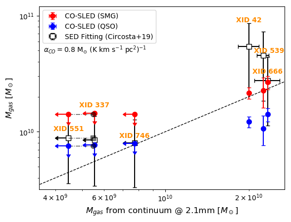
For the detected sources (XID 42, XID 539 and XID 666) the gas masses obtained from the dust emission are fully compatible (within 1) with those derived from both the SMG CO–SLED conversion factor and IR-SED fitting (Circosta et al. 2019). Moreover, for XID 42, Calistro Rivera et al. 2018 obtained a gas mass of 5 2 from the CO(3–2) line, which is in agreement with our SMG CO–SLED and continuum measurements (3) and SED fitting derived mass (1). XID 539 shows all masses compatible within 3 with the molecular mass of 1.6 found by Coppin et al. 2010 on the basis of CO(2–1) transition analysis. The lowest masses are the those derived using the QSO CO–SLED, as a consequence of the higher line ratios (Carilli & Walter 2013), which in turn lead to lower values. Finally we note that for the undetected sources the gas masses derived by Circosta et al. 2019 from the SED fitting are in agreement (within 1) with the upper limits derived in this work.
In order take in account also a Galactic , we calculate the gas mass (still accounting for the atomic gas mass as 1/5 of the molecular gas mass) from the CO emission assuming = 6.5, as used by Scoville et al. 2016 to calibrate their relation (this also includes a factor of 1.36 with respect to the molecular hydrogen gas mass, accounting for the mass of heavier elements). Then, we calculate the molecular gas mass directly from via the factor (we note that assumed by Scoville et al. 2016 to derive the – and used to calibrate – slightly differs from that assumed in this work, that is ; this difference is negligible considering the large uncertainty on the other assumed conversion factors). The results are shown in Fig. 5. Because of the linear scaling of the gas mass with at a given , the CO-derived gas masses in Fig. 5 are a factor 6.5/0.8 = 8.1 times higher than those shown in Fig. 4. For the detected sources, we found that the gas mass derived from the continuum is comprised in the range of values encompassed by the gas masses derived assuming the two CO–SLEDs, and in general that they are all compatible within 3. The consistency between these measurements is further increased if one considers that an additional 25% uncertainty is present in the conversion factor.

5.4 Notes on the morphology of the sources
XID 42 shows a gradient along one direction in the velocity map, at least with a beam separation, suggesting the presence of a differential kinematic structure. In addition, its velocity dispersion is mostly concentrated in the central core of the galaxy. Calistro Rivera et al. 2018 have inferred its inclination angle () from the axial ratio of the CO(3–2) emission assuming a disk–like geometry, while Rybak et al. 2019 have fit the [C ii] emission with a rotating disk model. We investigated the observation of the source carried out by the HST in the V band (GEMS tile ID: 27), corresponding to the rest–frame UV emission. In Fig. 6 we report the r-g-b image in which the red, green and blue channels correspond to the continuum dust emission, CO moment 0 and optical image, respectively. Originally the optical image was shifted by 0.2 arcsec from the center of the dust (and CO) emission in the northwest direction, in agreement with the astrometric error between ALMA and HST images shown by Dunlop et al. 2017. Thus, we corrected the HST image astrometry using the GAIA position measurements of the sources in the same field (Gaia Collaboration et al. 2016). After the correction the bulks of the stellar, dust and molecular gas emission coincide, within the beam resolution. The optical image shows a very irregular shape that, coupled with the significant shift of the CO(5–4) line with respect to the optical rest–frame (Fig. 2), confirms the peculiar properties of this source. Therefore, we point out that XID 42 may not be securely associated to a regular rotating disk morphology, and further high-resolution observations are required to draw definitive conclusions on its nature.

Indications of a rotating system for XID 666 come from the observed velocity gradient that is clearly distributed along a defined direction (moments 1, Fig. 3), and from the line that shows a double–peaked feature (Fig. 2), with the blue and red–shifted peaks that actually correspond to two different emitting regions. However, the very asymmetric distribution of the two peaks suggests the possibility that XID 666 could actually be a blend of two merging systems. As a support to this interpretation, the moment 2 map (Fig. 3) shows that the velocity dispersion is mostly concentrated in two clumps, a bigger one located in the innermost region of the source, and a smaller one located southeast from the main clump. Even improving the resolution during the imaging (i.e., lowering the robust weighting), we could not unambiguously distinguish the presence of two different sources, and future observations at higher resolution will help to reject or confirm this interesting prospect.
For XID 539 it would be critical to assess the presence of a rotating system, due to both the spectral shape (Fig. 2) and low S/N per channel (¡ 5 in the peak). However, the velocity maps suggest the presence of a differential kinematic structure in one direction, at least with a beam separation between the red and blue–shifted region, and the velocity dispersion is confined in a relatively small region concentrated at the center of the source (moments 1 and 2, Fig. 3). In addition, De Breuck et al. 2014, using ALMA data with a resolution of 0.5”, demonstrated that the [C ii] emission is well described by a rotating disk model with a similar position angle.
Despite these indications of rotating systems, we could not properly constrain a realistic disk-like model for the sources, due to the large uncertainties on the sizes. Instead, in order to derive the column densities in Sec. 5.5, we consider only a simple uniform spherical geometry. However, we point out that assuming a more compact morphology would simply result in compressing the same amount of gas reservoir in a smaller volume, implying higher densities. Future observations at higher resolution will dramatically reduce the uncertainties on the sizes and in turn on all the size-dependent quantities such as the ISM density.
5.5 Column density associated with the ISM
The obtained masses and sizes reveal that a large reservoir of gas is confined in a few kiloparsec region, in agreement with the literature for SMG in the same redshift range (Carilli & Walter 2013; Bothwell et al. 2013, e.g.,). We derived the ISM density as , where is the gas mass derived either from the CO line (using CO–SLEDs) or the continuum emission (using the Scoville et al. 2016 relation), assuming = 0.8 in both the cases, and where V is the volume of a given geometrical model of the source. In order to obtain the number density of the hydrogen atoms, we further divide by the proton mass. Then, we calculated the column density toward the nucleus multiplying the number density by the length of the optical path, from the center of the source toward the galaxy outskirts.
We present a homogeneous spherical model for every source, which is the simplest assumption because it is symmetrical in any direction and independent on the inclination angle. Given the 3 upper limit to the gas mass for the undetected sources, we derived a 3 upper limit on the column densities as well. As the source diameter we considered the mean value between the major and minor axis of the Gaussian ellipse fit reported in the top panel of Table 5; as path length we assumed half of the diameter. In Table 7 we report the gas column densities (column 8) for the spherical model using the gas mass derived with the various methods indicated in column 5 of the same table. In column 11 we report the X-ray column density derived by Circosta et al. 2019. The ISM vs. X-ray column densities plot is shown in Fig. 7.
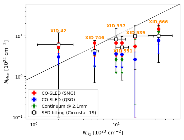
All the column densities derived through the different methods show values similar to (up to ), suggesting that the host galaxy can provide a significant amount of the column density toward the central AGN. These results are also in agreement with the column densities found by Circosta et al. 2019 from the masses obtained by the IR-SED fitting. We stress that if we consider the gas masses derived from the high-J CO lines and from the continuum emission using and , respectively, the ISM column density would increase by a factor of 8.1.
Column description: (1) ID of the sources. (2) Integrated flux of the observed transition (in units of Jy km ), derived multiplying the flux density (second column of Table 4) by the FWHM of the line (third column in Table 3, for XID 666 we assumed that the line width is equal to the sum of the FWHM of the two line components). For the undetected sources we assumed a line width of 400 km/s. (3) Luminosity of the observed transition derived from . (4) Flux density at 850(1+z) m (in units of Jy), derived from the observed 2.1 mm flux density assuming a modified black body (MBB) model. (5) Conversion methods adopted to compute the CO(1–0) transition luminosity : “SMG CO–SLED” and “QSO CO–SLED” refer to two conversion factors, typical for SMGs and QSOs, respectively, between and (see text), while “MBB”exploits the relation found by Scoville et al. 2016. (6) Derived CO(1–0) transition luminosities. (7) Total gas mass assuming a CO luminosity-to-molecular gas mass () conversion factor , and considering the atomic gas mass equal to (Calura et al. 2014). (8) Column densities in the spherical geometry, assuming as a path length of the light the radius of the sphere. (9) (10) (11) Gas mass, infrared SED-fitting column density, and X-ray spectral fitting column density, respectively, derived by Circosta et al. 2019.
The upper limits for the undetected sources are given at the 3 upper level.
| XID | Method | |||||||||
|---|---|---|---|---|---|---|---|---|---|---|
| (1) | (2) | (3) | (4) | (5) | (6) | (7) | (8) | (9) | (10) | (11) |
| SMG CO–SLED | 5.2 | |||||||||
| 42 | QSO CO–SLED | 3.0 | ||||||||
| MBB | ||||||||||
| SMG CO–SLED | ||||||||||
| 337 | QSO CO–SLED | 3.6 | ||||||||
| MBB | ||||||||||
| SMG CO–SLED | 5.5 | |||||||||
| 539 | QSO CO–SLED | 2.6 | ||||||||
| MBB | ||||||||||
| SMG CO–SLED | ||||||||||
| 551 | QSO CO–SLED | 3.5 | ||||||||
| MBB | ||||||||||
| SMG CO–SLED | 14.6 | |||||||||
| 666 | QSO CO–SLED | 7.7 | ||||||||
| MBB | ||||||||||
| SMG CO–SLED | 6.6 | |||||||||
| 746 | QSO CO–SLED | 3.7 | ||||||||
| MBB |
The spherical model likely underestimates the source density, since it distributes the mass on a larger volume than models based on more compact and realistic geometries (e.g., disk–like). Given the derived column densities (23–24) for the spherical model, we infer that a more compact morphology can produce even larger column densities, depending on the inclination angle and gas mass profile. This means that the host galaxy ISM may contribute to the nuclear obscuration up to the Compton-thick regime, especially adopting a high value for .
5.6 Dynamical mass
Given the indications of a rotating structure for the detected sources (Sec. 5.4), we derive the dynamical masses in the idealized case of a simple uniform thin disk geometry, where the diameter corresponds to the major axis and the inclination angle (defined with respect to the perpendicular to the line of sight, north to south) is derived from the axial ratio. We assume = , , for XID 42, XID 539 and XID 666, respectively. For XID 42 and XID 539 we derive the dynamical masses from the FWHM (v) of the CO lines obtained from the spectral fitting reported in Table 3, exploiting the following relation adapted from Wang et al. 2013, which assumes a ratio of 0.75 between the maximum projected circular velocity and v:
For XID 666 we resolve the double peak of the line, thus we directly derive the dynamical mass from = km/s, calculated as the half of the peak separation, assuming that is the distance at which the circular velocity flattens:
We found , , for XID 42, XID 539 and XID 666, respectively. These values are about one order of magnitude lower than the values previously found for SMG at z2 based on the study of resolved and unresolved CO kinematics (Tacconi et al. 2008; Swinbank et al. 2010; Bothwell et al. 2013) and than the baryonic mass calculated as , where are the stellar masses obtained by the SED fitting (Circosta et al. 2019) which are equal to , , for XID 42, XID 539 and XID 666, respectively. We stress that, for XID 539, De Breuck et al. 2014 and Coppin et al. 2010 found in agreement with the value derived in this work. De Breuck et al. 2014 have assumed different inclination angles (29∘, 50∘ and 53∘), while in Coppin et al. 2010 an angle was assumed, as appropriate for randomly inclined disks in a sample of galaxies. Such discrepancy could be attributed either to an overestimate of the stellar mass by the SED fitting or to an underestimate of v and , given the sensitivity limitation of the observations. As for XID 666, we assumed that is equal to the half of the distance of the peaks and that the disk diameter is the distance at which the velocity profile flattens, but due to the large uncertainty on the source geometry and size it is not possible to securely determine this distance. It is also likely that the stellar mass has been derived considering a different emitting area with respect to the molecular gas. Finally we note that the 30% error on the stellar masses reported in Circosta et al. 2019 is indicative only of the statistical error given the assumed Salpeter Initial Mass Function (Salpeter 1955, IMF,), and the systematic error due to different choices of IMF are likely much larger. By assuming a Chabrier IMF (Chabrier 2003) the resulting stellar masses would be a factor 1.7 smaller, leading to a lower discrepancy in the / ratio.
6 Summary and conclusions
Exploiting ALMA data we analyzed the high-J CO and the dust emission of a sample of six star forming galaxies hosting a heavily obscured () AGN in the redshift range 2.5 ¡ ¡ 4.7 in the CDF–S. We detect both the line and continuum emissions for three sources, for which we extracted the flux densities and sizes in order to characterize their masses, gas densities and column densities, and evaluate to what extent the host galaxy ISM can contribute to the central AGN obscuration. Our results are summarized as follows.
- -
We fit the CO line and continuum emission in both the brightness and visibility spaces with a 2–D Gaussian model, finding that all sources are extremely compact objects. The CO emission, tracing the molecular gas component, is contained in regions with major axis in the range 2.1 – 3 kpc. The continuum emission, tracing the dust component, is produced in somewhat smaller regions, with major axes that are 10 – 30 % smaller than those derived from the CO emission. This difference in size can be explained by a radial decrease of the gas column density and dust temperature (Calistro Rivera et al. 2018), but we cannot exclude that it could be attributed to the sensitivity limit of the observations.
- -
We analyzed the spectra of the detected sources and performed a Gaussian fit to the lines. For one of these sources (XID 666) we found a double–peaked feature that we ascribe to a rotating disk-like morphology. However, given the strong asymmetry of the line shape (Fig. 2, bottom panel) and the dispersion velocity mainly distributed in two separated clumps, we cannot exclude that XID 666 is actually an unresolved merger of two different systems. XID 42 also shows indication of a rotating structure, even if it cannot be securely associated to a regular disk shape: the line is red-shifted by 500 km/s with respect to the optical rest–frame velocity and the HST image (V–band, Fig. 6), that traces the UV rest–frame stellar emission, shows a very irregular morphology. These features make XID 42 the most peculiar target among the sample, and observations at higher resolution ( 0.1”) would be necessary to cover the source with a sufficient ( 5-6) number of beams, and unveil whether its kinematics points to relaxed system or to a chaotic, merging, structure.
- -
We calculated the gas mass as , assuming (Calura et al. 2014). The molecular gas mass was firstly derived from the high-J CO detected lines assuming two different CO–SLEDs typical for SMGs and QSOs to obtain , and then assuming a – conversion factor . We obtained masses in the range , in agreement with those derived by Circosta et al. 2019 from the SED fitting. Secondly, we derived the molecular gas masses from the continuum emission on the basis of the – empirical relation found by Scoville et al. 2016, using a modified black–body model to calculate and then again = 0.8 to obtain the gas masses. We found that these masses are fully in agreement (within 1) with those derived from the CO line emission. In order to encompass the uncertainty on , we also calculated the gas masses from the CO lines using = 6.5, and then compared these values with those obtained from the direct Scoville et al. 2016 relation and , which is based on the assumption of the same , finding that they are in good agreement. This corresponds to an increase of the gas masses (a factor of 8.1) and, as a consequence, in a more pronounced contribution of the ISM to the nuclear obscuration.
- -
We investigated the contribution of the host galaxy to the obscuration of the AGN by comparing the column density derived from the ISM masses with that () derived from the X-ray spectral fitting (Circosta et al. 2019). As for the source geometry, we assumed a uniform spherical model for all the sources. We found that is similar to (), and conclude that the host galaxy can significantly affect the obscuration of the central engine. All the are also comparable to the column densities derived by Circosta et al. 2019 from the IR-SED fitting. We point out that despite the large number of assumptions, the values derived from three independent measurements (i.e., CO line, dust continuum and SED fitting), are in agreement with each other and with . This result strongly supports a scenario in which a substantial fraction of the obscuration may be produced on large (kpc) scales, at least for these FIR-bright objects characterized by a large gas reservoir confined in a very compact volume. Since the spherical model likely underestimates the ISM density, we point out that a more realistic (disk-like) geometry, compressing the gas mass in a smaller volume, would result in larger density; depending on the inclination angle of the disk and the gas distribution, this may produce column densities that can significantly affect the obscuration even in heavily Compton-thick AGN ().
- -
From the continuum emission we derived the dust mass, assuming a modified black body law in the optically thin regime. We found that the dust masses are in the range .
- -
We derived the dynamical masses for the three detected sources, whose values are in the range . These masses are one order of magnitude lower than the sum of the stellar (Circosta et al. 2019) and gas masses, and consistent with those derived in previous work for XID 539, assuming different inclination angles (Coppin et al. 2010; De Breuck et al. 2014). Such discrepancy could be attributed to an overestimate of the stellar mass by the SED fitting or to an underestimate of the FWHM of the line and the gas component size (given the sensitivity limitation of the observations). Moreover, the stellar mass may be derived considering a different emitting area with respect to the molecular gas. Finally, we note that the scatter of the stellar masses derived by Circosta et al. 2019 does not take into account different assumptions for the IMF. Indeed, by assuming a Chabrier IMF the stellar masses reduce of a factor 1.7, leading to a smaller discrepancy between and .
From the analysis of our sample, we conclude that SMGs environment is characterized by an extremely dense ISM confined in few kiloparsec. In such conditions, the ISM can produce column densities that contribute to the obscuration of the central AGN up to the Compton-thick regime. In addition, the sources’ velocity gradient indicates the presence of a rotating system, even though some of their morphological features suggest a more complex structure, possibly associated with mergers.
Acknowledgements.
QD acknowledges A. Peca and G. Sabatini for all the support during the long journey, and R. Decarli, M. Mignoli and G. Iorio for the very helpful discussions. CC acknowledges support from the IMPRS on Astrophysics at the LMU (Munich). FV acknowledges financial support from CONICYT and CASSACA through the Fourth call for tenders of the CAS-CONICYT Fund and from CONICYT grants Basal-CATA AFB-170002. This paper makes use of the following ALMA data: 2015.1.01205.S. ALMA is a partnership of ESO (representing its member states), NSF (USA) and NINS (Japan), together with NRC (Canada), MOST and ASIAA (Taiwan), and KASI (Republic of Korea), in cooperation with the Republic of Chile. The Joint ALMA Observatory is operated by ESO, AUI/NRAO and NAOJ.References
- Barro et al. (2014) Barro, G., Faber, S. M., Pérez-González, P. G., et al. 2014, ApJ, 791, 52
- Bennett et al. (2014) Bennett, C. L., Larson, D., Weiland, J. L., & Hinshaw, G. 2014, ApJ, 794, 135
- Blain et al. (2002) Blain, A. W., Smail, I., Ivison, R. J., Kneib, J.-P., & Frayer, D. T. 2002, Physics Reports, 369, 111
- Bolatto et al. (2013) Bolatto, A. D., Wolfire, M., & Leroy, A. K. 2013, ARAA, 51, 207
- Bothwell et al. (2013) Bothwell, M. S., Smail, I., Chapman, S. C., et al. 2013, MNRAS, 429, 3047
- Bournaud et al. (2011) Bournaud, F., Chapon, D., Teyssier, R., et al. 2011, ApJ, 730, 4
- Burlon et al. (2011) Burlon, D., Ajello, M., Greiner, J., et al. 2011, ApJ, 728, 58
- Calistro Rivera et al. (2018) Calistro Rivera, G., Hodge, J. A., Smail, I., et al. 2018, ApJ, 863, 56
- Calura et al. (2014) Calura, F., Gilli, R., Vignali, C., et al. 2014, MNRAS, 438, 2765
- Carilli & Walter (2013) Carilli, C. L. & Walter, F. 2013, ARAA, 51, 105
- Carniani et al. (2018) Carniani, S., Maiolino, R., Amorin, R., et al. 2018, MNRAS, 478, 1170
- Casasola et al. (2017) Casasola, V., Cassarà, L. P., Bianchi, S., et al. 2017, A&A, 605, A18
- Cassata et al. (2011) Cassata, P., Giavalisco, M., Guo, Y., et al. 2011, ApJ, 743, 96
- Chabrier (2003) Chabrier, G. 2003, PASP, 115, 763
- Chen et al. (2015) Chen, C.-C., Smail, I., Swinbank, A. M., et al. 2015, ApJ, 799, 194
- Cimatti et al. (2008) Cimatti, A., Cassata, P., Pozzetti, L., et al. 2008, A&A, 482, 21
- Circosta et al. (2019) Circosta, C., Vignali, C., Gilli, R., et al. 2019, A&A, 623, A172
- Comastri et al. (2011) Comastri, A., Ranalli, P., Iwasawa, K., et al. 2011, A&A, 526, L9
- Condon (1997) Condon, J. J. 1997, pASP, 109, 166
- Conley et al. (2011) Conley, A., Cooray, A., Vieira, J. D., et al. 2011, ApJl, 732, L35
- Coppin et al. (2010) Coppin, K. E. K., Chapman, S. C., Smail, I., et al. 2010, MNRAS, 407, L103
- Daddi et al. (2010) Daddi, E., Bournaud, F., Walter, F., et al. 2010, ApJ, 713, 686
- Daddi et al. (2015) Daddi, E., Dannerbauer, H., Liu, D., et al. 2015, A&A, 577, A46
- De Breuck et al. (2014) De Breuck, C., Williams, R. J., Swinbank, M., et al. 2014, A&A, 565, A59
- Dekel et al. (2009) Dekel, A., Sari, R., & Ceverino, D. 2009, ApJ, 703, 785
- Del Moro et al. (2016) Del Moro, A., Alexander, D. M., Bauer, F. E., et al. 2016, MNRAS, 456, 2105
- Draine & Li (2007) Draine, B. T. & Li, A. 2007, ApJ, 657, 810
- Dunlop et al. (2017) Dunlop, J. S., McLure, R. J., Biggs, A. D., et al. 2017, MNRAS, 466, 861
- Engel et al. (2010) Engel, H., Tacconi, L. J., Davies, R. I., et al. 2010, ApJ, 724, 233
- Feltre et al. (2012) Feltre, A., Hatziminaoglou, E., Fritz, J., & Franceschini, A. 2012, MNRAS, 426, 120
- Feruglio et al. (2011) Feruglio, C., Daddi, E., Fiore, F., et al. 2011, ApJl, 729, L4
- Gaia Collaboration et al. (2016) Gaia Collaboration, Brown, A. G. A., Vallenari, A., et al. 2016, A&A, 595, A2
- Gawiser & MUSYC Collaboration (2003) Gawiser, E. & MUSYC Collaboration. 2003, in Bulletin of the American Astronomical Society, Vol. 35, American Astronomical Society Meeting Abstracts, 1249
- Genzel et al. (2010) Genzel, R., Tacconi, L. J., Gracia-Carpio, J., et al. 2010, MNRAS, 407, 2091
- Genzel et al. (2015) Genzel, R., Tacconi, L. J., Lutz, D., et al. 2015, ApJ, 800, 20
- Giavalisco et al. (2004) Giavalisco, M., Ferguson, H. C., Koekemoer, A. M., et al. 2004, ApJl, 600, L93
- Gilli et al. (2014) Gilli, R., Norman, C., Vignali, C., et al. 2014, A&A, 562, A67
- Gilli et al. (2011) Gilli, R., Su, J., Norman, C., et al. 2011, Apjl, 730, L28
- Grogin et al. (2011) Grogin, N. A., Kocevski, D. D., Faber, S. M., et al. 2011, ApJs, 197, 35
- Gruppioni et al. (2013) Gruppioni, C., Pozzi, F., Rodighiero, G., et al. 2013, MNRAS, 432, 23
- Häussler et al. (2007) Häussler, B., McIntosh, D. H., Barden, M., et al. 2007, ApJs, 172, 615
- Hodge et al. (2012) Hodge, J. A., Carilli, C. L., Walter, F., et al. 2012, ApJ, 760, 11
- Hodge et al. (2013) Hodge, J. A., Karim, A., Smail, I., et al. 2013, ApJ, 768, 91
- Hodge et al. (2016) Hodge, J. A., Swinbank, A. M., Simpson, J. M., et al. 2016, ApJ, 833, 103
- Hopkins & Beacom (2006) Hopkins, A. M. & Beacom, J. F. 2006, ApJ, 651, 142
- Hsu et al. (2014) Hsu, L.-Y., Stockton, A., & Shih, H.-Y. 2014, ApJ, 796, 92
- Ikarashi et al. (2015) Ikarashi, S., Ivison, R. J., Caputi, K. I., et al. 2015, ApJ, 810, 133
- Ivison et al. (2013) Ivison, R. J., Swinbank, A. M., Smail, I., et al. 2013, ApJ, 772, 137
- Kaasinen et al. (2019) Kaasinen, M., Scoville, N., Walter, F., et al. 2019, ApJ, 880, 15
- Kirkpatrick et al. (2019) Kirkpatrick, A., Sharon, C., Keller, E., & Pope, A. 2019, ApJ, 879, 41
- Lapi et al. (2018) Lapi, A., Pantoni, L., Zanisi, L., et al. 2018, ApJ, 857, 22
- Lapi et al. (2014) Lapi, A., Raimundo, S., Aversa, R., et al. 2014, ApJ, 782, 69
- Luo et al. (2017) Luo, B., Brandt, W. N., Xue, Y. Q., et al. 2017, ApJs, 228, 2
- Madau & Dickinson (2014) Madau, P. & Dickinson, M. 2014, ARA&A, 52, 415
- Magdis et al. (2012) Magdis, G. E., Daddi, E., Béthermin, M., et al. 2012, ApJ, 760, 6
- Magnelli et al. (2012) Magnelli, B., Lutz, D., Santini, P., et al. 2012, A&A, 539, A155
- Magnelli et al. (2013) Magnelli, B., Popesso, P., Berta, S., et al. 2013, A&A, 553, A132
- Mainieri et al. (2005) Mainieri, V., Rigopoulou, D., Lehmann, I., et al. 2005, MNRAS, 356, 1571
- Massardi et al. (2018) Massardi, M., Enia, A. F. M., Negrello, M., et al. 2018, A&A, 610, A53
- Matthee et al. (2017) Matthee, J., Sobral, D., Boone, F., et al. 2017, ApJ, 851, 145
- Mingozzi et al. (2018) Mingozzi, M., Vallini, L., Pozzi, F., et al. 2018, MNRAS, 474, 3640
- Nagao et al. (2012) Nagao, T., Maiolino, R., De Breuck, C., et al. 2012, A&A, 542, L34
- Norman et al. (2002) Norman, C., Hasinger, G., Giacconi, R., et al. 2002, ApJ, 571, 218
- Oliver et al. (2012) Oliver, S. J., Bock, J., Altieri, B., et al. 2012, MNRAS, 424, 1614
- Papadopoulos et al. (2012) Papadopoulos, P. P., van der Werf, P., Xilouris, E., Isaak, K. G., & Gao, Y. 2012, ApJ, 751, 10
- Pentericci et al. (2016) Pentericci, L., Carniani, S., Castellano, M., et al. 2016, ApJ, 829, L11
- Perna et al. (2018) Perna, M., Sargent, M. T., Brusa, M., et al. 2018, A&A, 619, A90
- Pozzi et al. (2017) Pozzi, F., Vallini, L., Vignali, C., et al. 2017, MNRAS, 470, L64
- Rangwala et al. (2011) Rangwala, N., Maloney, P. R., Glenn, J., et al. 2011, ApJ, 743, 94
- Rigopoulou et al. (2009) Rigopoulou, D., Mainieri, V., Almaini, O., et al. 2009, MNRAS, 400, 1199
- Rix et al. (2004) Rix, H.-W., Barden, M., Beckwith, S. V. W., et al. 2004, ApJs, 152, 163
- Rybak et al. (2019) Rybak, M., Calistro Rivera, G., Hodge, J. A., et al. 2019, ApJ, 876, 112
- Saintonge et al. (2018) Saintonge, A., Wilson, C. D., Xiao, T., et al. 2018, MNRAS, 481, 3497
- Salpeter (1955) Salpeter, E. E. 1955, ApJ, 121, 161
- Santini et al. (2014) Santini, P., Maiolino, R., Magnelli, B., et al. 2014, A&A, 562, A30
- Schreiber et al. (2015) Schreiber, C., Pannella, M., Elbaz, D., et al. 2015, A&A, 575, A74
- Scoville et al. (2016) Scoville, N., Sheth, K., Aussel, H., et al. 2016, Apj, 820, 83
- Simpson et al. (2014) Simpson, J. M., Swinbank, A. M., Smail, I., et al. 2014, ApJ, 788, 125
- Solomon et al. (1992) Solomon, P. M., Downes, D., & Radford, S. J. E. 1992, ApJ, 398, L29
- Solomon & Vanden Bout (2005) Solomon, P. M. & Vanden Bout, P. A. 2005, ARA&A, 43, 677
- Swinbank et al. (2014) Swinbank, A. M., Simpson, J. M., Smail, I., et al. 2014, MNRAS, 438, 1267
- Swinbank et al. (2010) Swinbank, A. M., Smail, I., Chapman, S. C., et al. 2010, MNRAS, 405, 234
- Szokoly et al. (2004) Szokoly, G. P., Bergeron, J., Hasinger, G., et al. 2004, ApJs, 155, 271
- Tacconi et al. (2018) Tacconi, L. J., Genzel, R., Saintonge, A., et al. 2018, ApJ, 853, 179
- Tacconi et al. (2008) Tacconi, L. J., Genzel, R., Smail, I., et al. 2008, ApJ, 680, 246
- Talia et al. (2018) Talia, M., Pozzi, F., Vallini, L., et al. 2018, MNRAS, 476, 3956
- Urry & Padovani (1995) Urry, C. M. & Padovani, P. 1995, PASP, 107, 803
- Vallini et al. (2019) Vallini, L., Tielens, A. G. G. M., Pallottini, A., et al. 2019, MNRAS, 490, 4502
- Vito et al. (2018) Vito, F., Brandt, W. N., Yang, G., et al. 2018, MNRAS, 473, 2378
- Vito et al. (2013) Vito, F., Vignali, C., Gilli, R., et al. 2013, MNRAS, 428, 354
- Wang et al. (2013) Wang, R., Wagg, J., Carilli, C. L., et al. 2013, ApJ, 773, 44
- Weiß et al. (2007) Weiß, A., Downes, D., Walter, F., & Henkel, C. 2007, in Astronomical Society of the Pacific Conference Series, Vol. 375, From Z-Machines to ALMA: (Sub)Millimeter Spectroscopy of Galaxies, ed. A. J. Baker, J. Glenn, A. I. Harris, J. G. Mangum, & M. S. Yun, 25
- Xue et al. (2011) Xue, L., Sa̧dowski, A., Abramowicz, M. A., & Lu, J.-F. 2011, ApJs, 195, 7