The isotropic Cosserat shell model including terms up to $O(h^{5})$.
Part II: Existence of minimizers

In this paper, for $a,b\in\mathbb{R}^{n}$ we let $\bigl\langle{a},{b}\bigr\rangle_{\mathbb{R}^{n}}$ denote the scalar product on $\mathbb{R}^{n}$ with associated (squared) vector norm $\lVert a\rVert_{\mathbb{R}^{n}}^{2}=\bigl\langle{a},{a}\bigr\rangle_{\mathbb{R}^{n}}$ The standard Euclidean scalar product on the set of real $n\times{m}$ second order tensors $\mathbb{R}^{n\times{m}}$ is given by $\bigl\langle{X},{Y}\bigr\rangle_{\mathbb{R}^{n\times{m}}}={\rm tr}(X\,Y^{T})$, and thus the (squared) Frobenius tensor norm is $\lVert{X}\rVert^{2}_{\mathbb{R}^{n\times{m}}}=\bigl\langle{X},{X}\bigr\rangle_{\mathbb{R}^{n\times{m}}}$. In the following we omit the subscripts $\mathbb{R}^{n},\mathbb{R}^{n\times{m}}$. The identity tensor on $\mathbb{R}^{n\times n}$ will be denoted by ${\boldsymbol{\mathbbm{1}}}_{n}$, so that ${\rm tr}({X})=\bigl\langle{X},{{\boldsymbol{\mathbbm{1}}}}_{n}\bigr\rangle$. We let ${\rm Sym}(n)$ and ${\rm Sym}^{+}(n)$ denote the symmetric and positive definite symmetric tensors, respectively. We adopt the usual abbreviations of Lie-group theory, e.g., ${\rm GL}(n)=\{X\in\mathbb{R}^{n\times n}\;|\det({X})\neq 0\}$ the general linear group, ${\rm SO}(n)=\{X\in{\rm GL}(n)|X^{T}X={\boldsymbol{\mathbbm{1}}}_{n},\det({X})=1\}$ with corresponding Lie-algebras $\mathfrak{so}(n)=\{X\in\mathbb{R}^{n\times n}\;|X^{T}=-X\}$ of skew symmetric tensors and $\mathfrak{sl}(n)=\{X\in\mathbb{R}^{n\times n}\;|\,{\rm tr}({X})=0\}$ of traceless tensors. For all $X\in\mathbb{R}^{n\times n}$ we set ${\rm sym}\,X\,=\frac{1}{2}(X+X^{T})\in{\rm Sym}(n)$, ${\rm skew}\,X\,=\frac{1}{2}(X-X^{T})\in\mathfrak{so}(n)$ and the deviatoric part ${\rm dev}\,X\,=X-\frac{1}{n}\;\,{\rm tr}(X)\,{\boldsymbol{\mathbbm{1}}}_{n}\in\mathfrak{sl}(n)$ and we have the orthogonal Cartan-decomposition of the Lie-algebra $\mathfrak{gl}(n)$ on the vector space $\mathbb{R}^{n\times n}$, $\mathfrak{gl}(n)=\{\mathfrak{sl}(n)\cap{\rm Sym}(n)\}\oplus\mathfrak{so}(n)\oplus\mathbb{R}\!\cdot\!{\boldsymbol{\mathbbm{1}}}_{n},$ $X={\rm dev}\,{\rm sym}\,X\,+{\rm skew}\,X\,+\frac{1}{n}\,{\rm tr}(X)\,{\boldsymbol{\mathbbm{1}}}_{n}\,.$ A matrix having the three columns vectors $A_{1},A_{2},A_{3}$ will be written as $(A_{1}\,|\,A_{2}\,|\,A_{3}).$ We make use of the operator $\mathrm{axl}:\mathfrak{so}(3)\to\mathbb{R}^{3}$ associating with a matrix $A\in\mathfrak{so}(3)$ the vector $\mathrm{axl}{\,A}\coloneqq(-A_{23},A_{13},-A_{12})^{T}$. The inverse of the operator $\mathrm{axl}:\mathfrak{so}(3)\to\mathbb{R}^{3}$ is denoted by $\mathrm{anti}:\mathbb{R}^{3}\to\mathfrak{so}(3)$.

Let $\Omega$ be an open domain of $\mathbb{R}^{3}$. The usual Lebesgue spaces of square integrable functions, vector or tensor fields on $\Omega$ with values in $\mathbb{R}$, $\mathbb{R}^{3}$, $\mathbb{R}^{3\times 3}$ or ${\rm SO}(3)$, respectively will be denoted by ${\rm L}^{2}(\Omega;\mathbb{R})$, ${\rm L}^{2}(\Omega;\mathbb{R}^{3})$, ${\rm L}^{2}(\Omega;\mathbb{R}^{3\times 3})$ and ${\rm L}^{2}(\Omega;{\rm SO}(3))$, respectively. Moreover, we use the standard Sobolev spaces ${\rm H}^{1}(\Omega;\mathbb{R})$ [1, 22, 26] of functions $u$. For vector fields $u=\left(u_{1},u_{2},u_{3}\right)^{T}$ with $u_{i}\in{\rm H}^{1}(\Omega)$, $i=1,2,3$, we define $\nabla\,u:=\left(\nabla\,u_{1}\,|\,\nabla\,u_{2}\,|\,\nabla\,u_{3}\right)^{T}.$ The corresponding Sobolev-space will be denoted by ${\rm H}^{1}(\Omega;\mathbb{R}^{3})$. If a tensor $Q:\Omega\to{\rm SO}(3)$ has the components in ${\rm H}^{1}(\Omega;\mathbb{R})$, then we mark this by writing $Q\in{\rm H}^{1}(\Omega;{\rm SO}(3))$. When writting the norm in the corresponding Sobolev-space we will specify the space in subscript. The space will be omitted only when the Frobenius norm or scalar product is considered.

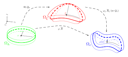
Let $\Omega_{\xi}\subset\mathbb{R}^{3}$ be a three-dimensional shell-like thin domain. In a fixed standard base $e_{1},e_{2},e_{3}$ of $\mathbb{R}^{3}$, a generic point of $\Omega_{\xi}$ will be denoted by $(\xi_{1},\xi_{2},\xi_{3})$. The elastic material constituting the shell is assumed to be homogeneous and isotropic and the reference configuration $\Omega_{\xi}$ is assumed to be a natural state. The deformation of the body occupying the domain $\Omega_{\xi}$ is described by a vector map $\varphi_{\xi}:\Omega_{\xi}\subset\mathbb{R}^{3}\rightarrow\mathbb{R}^{3}$ (called deformation) and by a microrotation tensor $\overline{R}_{\xi}:\Omega_{\xi}\subset\mathbb{R}^{3}\rightarrow{\rm SO}(3)\,.$ We denote the current configuration (deformed configuration) by $\Omega_{c}:=\varphi_{\xi}(\Omega_{\xi})\subset\mathbb{R}^{3}$, see Figure 1.

In what follows, we consider the fictitious Cartesian (planar) configuration $\Omega_{h}$ of the body. This parameter domain $\Omega_{h}\subset\mathbb{R}^{3}$ is a right cylinder of the form

where $\omega\subset\mathbb{R}^{2}$ is a bounded domain with Lipschitz boundary $\partial\omega$ and the constant length $h>0$ is the thickness of the shell. For shell–like bodies we consider the domain $\Omega_{h}$ to be thin, i.e., the thickness $h$ is small. We assume furthermore that there exists a $C^{1}$-diffeomorphism $\Theta:\mathbb{R}^{3}\rightarrow\mathbb{R}^{3}$ in the specific form

where $y_{0}:\omega\to\mathbb{R}^{3}$ is a function of class $C^{2}(\omega)$, so that $\Theta$ maps the fictitious planar Cartesian parameter space $\Omega_{h}$ onto the initially curved reference configuration of the shell $\Theta(\Omega_{h})=\Omega_{\xi}$, $\Theta(x_{1},x_{2},x_{3})=(\xi_{1},\xi_{2},\xi_{3})$. The diffeomorphism $\Theta$ maps the midsurface $\omega$ of the fictitious Cartesian parameter space $\Omega_{h}$ onto the midsurface $\omega_{\xi}=y_{0}(\omega)$ of $\Omega_{\xi}$ and $n_{0}$ is the unit normal vector to $\omega_{\xi}$. For simplicity and where no confusions may arise, we will omit subsequently to write explicitly the arguments $(x_{1},x_{2},x_{3})$ of the diffeomorphism $\Theta$ or we will specify only its dependence on $x_{3}$. We use the polar decomposition [37] of $\nabla_{x}\Theta(x_{3})$ and write $\nabla_{x}\Theta(x_{3})={Q}_{0}(x_{3})\,U_{0}(x_{3})\,,$ ${Q}_{0}(x_{3})={\rm polar}{(\nabla_{x}\Theta)(x_{3})}\in{\rm SO}(3),$ $U_{0}(x_{3})\in\rm{Sym}^{+}(3).$ Let us remark that

and that $\det(\nabla y_{0}|n_{0})=\sqrt{\det[(\nabla y_{0})^{T}\nabla y_{0}]}$ represents the surface element.

In the following, we consider the Weingarten map²² 2 We identify the Weingarten map, the first fundamental form and the second fundamental form with their associated matrices in the fixed base vector $e_{1},e_{2},e_{3}$. (or shape operator) on $y_{0}(\omega)$ defined by its associated matrix ${\rm L}_{y_{0}}\,=\,{\rm I}_{y_{0}}^{-1}{\rm II}_{y_{0}}\in\mathbb{R}^{2\times 2},$ where ${\rm I}_{y_{0}}:=[{\nabla y_{0}}]^{T}\,{\nabla y_{0}}\in\mathbb{R}^{2\times 2}$ and ${\rm II}_{y_{0}}:\,=\,-[{\nabla y_{0}}]^{T}\,{\nabla n_{0}}\in\mathbb{R}^{2\times 2}$ are the matrix representations of the first fundamental form (metric) and the second fundamental form, respectively. Then, the Gauß curvature ${\rm K}$ of the surface $y_{0}(\omega)$ is determined by ${\rm K}:=\,{\rm det}{({\rm L}_{y_{0}})}\,$ and the mean curvature $\,{\rm H}\,$ through $2\,{\rm H}\,:={\rm tr}({{\rm L}_{y_{0}}}).$ We also need the tensors defined by:

and the so-called alternator tensor ${\rm C}_{y_{0}}$ of the surface [52]

Now, let us define the map $\varphi:\Omega_{h}\rightarrow\Omega_{c},\ \varphi(x_{1},x_{2},x_{3})=\varphi_{\xi}(\Theta(x_{1},x_{2},x_{3})).$ We view $\varphi$ as a function which maps the fictitious planar reference configuration $\Omega_{h}$ into the deformed configuration $\Omega_{c}$. We also consider the elastic microrotation $\overline{Q}_{e,s}:\Omega_{h}\rightarrow{\rm SO}(3),\ \overline{Q}_{e,s}(x_{1},x_{2},x_{3}):=\overline{R}_{\xi}(\Theta(x_{1},x_{2},x_{3}))\,.$

In [21], by assuming that $\overline{Q}_{e,s}(x_{1},x_{2},x_{3})=\overline{Q}_{e,s}(x_{1},x_{2})$ and considering an 8-parameter quadratic ansatz in the thickness direction for the reconstructed total deformation $\varphi_{s}:\Omega_{h}\subset\mathbb{R}^{3}\rightarrow\mathbb{R}^{3}$ of the shell-like body, we have obtained a two-dimensional minimization problem in which the energy density is expressed in terms of the following tensor fields on the surface $\omega\,$

where $m:\omega\subset\mathbb{R}^{2}\to\mathbb{R}^{3}$ represents the deformation of the midsurface. When these measures vanish, the shell undergoes a rigid body motion. Indeed, $\mathcal{K}_{e,s}{=0}$ implies $\partial_{x_{1}}\overline{Q}_{e,s}=0$, $\partial_{x_{2}}\overline{Q}_{e,s}=0$, while $\mathcal{E}_{m,s}=0$ leads to $\nabla m=\overline{Q}_{e,s}\nabla y_{0}$. Since $\overline{Q}_{e,s}$ is constant and $m=\overline{Q}_{e,s}\,y_{0}+c$, where $c$ is a constant vector field, this means that the shell is in a rigid body motion with constants translation $c$ and constant rotation $\overline{Q}_{e,s}$.

In [21], we have obtained the following two-dimensional minimization problem for the deformation of the midsurface $m:\omega\,{\to}\,\mathbb{R}^{3}$ and the microrotation of the shell $\overline{Q}_{e,s}:\omega\,{\to}\,\textrm{SO}(3)$ solving on $\omega\,\subset\mathbb{R}^{2}$: minimize with respect to $(m,\overline{Q}_{e,s})$ the functional

where the membrane part $\,W_{\mathrm{memb}}\big(\mathcal{E}_{m,s}\big)\,$, the membrane–bending part $\,W_{\mathrm{memb,bend}}\big(\mathcal{E}_{m,s},\,\mathcal{K}_{e,s}\big)\,$ and the bending–curvature part $\,W_{\mathrm{bend,curv}}\big(\mathcal{K}_{e,s}\big)\,$ of the shell energy density are given by

with

The parameters $\mu$ and $\lambda$ are the Lamé constants of classical isotropic elasticity, $\kappa=\frac{2\,\mu+3\,\lambda}{3}$ is the infinitesimal bulk modulus, $b_{1},b_{2},b_{3}$ are non-dimensional constitutive curvature coefficients (weights), $\mu_{\rm c}\geq 0$ is called the Cosserat couple modulus and ${L}_{\rm c}>0$ introduces an internal length which is characteristic for the material, e.g., related to the grain size in a polycrystal. The internal length ${L}_{\rm c}>0$ is responsible for size effects in the sense that smaller samples are relatively stiffer than larger samples. If not stated otherwise, we assume that $\mu>0$, $\kappa>0$, $\mu_{\rm c}>0$, $b_{1}>0$, $b_{2}>0$, $b_{3}>0$. Here, $\mu\,L_{\rm c}^{2}$ plays the role of a dimensional agreement factor. Without loss of generality, we may assume that $0<b_{1}<1$, $0<b_{2}<1$, $0<b_{3}<1$. All constitutive coefficients are deduced from the three-dimensional formulation, without using any a posteriori fitting of some two-dimensional constitutive coefficients.

The potential of applied external loads $\overline{\Pi}(m,\overline{Q}_{e,s})$ appearing in (2.6) is expressed by

where $u(x_{1},x_{2})\,=\,m(x_{1},x_{2})-y_{0}(x_{1},x_{2})$ is the displacement vector of the midsurface, $\Pi_{\omega}(m,\overline{Q}_{e,s})$ is the total potential of the external surface loads $f$ and of the external applied body couples $\Lambda_{\omega}(\overline{Q}_{e,s})$, while $\Pi_{\gamma_{t}}(m,\overline{Q}_{e,s})$ is the total potential of the external boundary loads $t$ and of the external boundary couples $\Lambda_{\gamma_{t}}(\overline{Q}_{e,s})$. Here, $\gamma_{t}$ and $\gamma_{d}$ are nonempty subsets of the boundary of $\omega$ such that $\gamma_{t}\cup\gamma_{d}=\partial\omega$ and $\gamma_{t}\cap\gamma_{d}=\emptyset$ . On $\gamma_{t}$ we have considered traction boundary conditions, while on $\gamma_{d}$ we have the Dirichlet-type boundary conditions:

where the boundary conditions are to be understood in the sense of traces.

The functions $\Lambda_{\omega}\,,\Lambda_{\gamma_{t}}:{\rm L}^{2}(\omega,\textrm{SO}(3))\rightarrow\mathbb{R}$ are expressed in terms of the loads from the three-dimensional parental variational problem, see [21], and they are assumed to be continuous and bounded operators.

We will consider materials for which the Poisson ratio $\nu=\frac{\lambda}{2(\lambda+\mu)}$ and Young’s modulus $E=\frac{\mu(3\,\lambda+2\,\mu)}{\lambda+\mu}$ are such that $-\frac{1}{2}<\nu<\frac{1}{2}$ and $E>0\,.$ This assumption implies that $2\,\lambda+\mu>0$. Under these assumptions on the constitutive coefficients, together with the positivity of $\mu$, $\mu_{\rm c}$, $b_{1}$, $b_{2}$ and $b_{3}$, and the orthogonal Cartan-decomposition of the Lie-algebra $\mathfrak{gl}(3)$, with

it follows that there exists the positive constants $c_{1}^{+},c_{2}^{+},C_{1}^{+}$ and $C_{2}^{+}$ such that

Hence, we note

References

• [1] R.A. Adams. Sobolev Spaces., volume 65 of Pure and Applied Mathematics. Academic Press, London, 1. edition, 1975.
• [2] J. Badur and W. Pietraszkiewicz. On geometrically non-linear theory of elastic shells derived from pseudo-Cosserat continuum with constrained micro-rotations. In W. Pietraszkiewicz, editor, Finite Rotations in Structural Mechanics., pages 19–32. Springer, Berlin, 1986.
• [3] J.M. Ball. Convexity conditions and existence theorems in nonlinear elasticity. Arch. Rational Mech. Anal., 63:337–403, 1977.
• [4] M. Bîrsan. Inequalities of Korn’s type and existence results in the theory of Cosserat elastic shells. J. Elasticity, 90:227–239, 2008.
• [5] M. Bîrsan. Derivation of a refined 6-parameter shell model: Descent from the three-dimensional Cosserat elasticity using a method of classical shell theory. Math. Mech. Solids, doi.org/10.1177/1081286519900531, 2020.
• [6] M. Bîrsan, I.D. Ghiba, R.J. Martin, and P. Neff. Refined dimensional reduction for isotropic elastic Cosserat shells with initial curvature. Math. Mech. Solids, 24(12):4000–4019, 2019.
• [7] M. Bîrsan and P. Neff. Existence of minimizers in the geometrically non-linear 6-parameter resultant shell theory with drilling rotations. Math. Mech. Solids, 19(4):376–397, 2014.
• [8] M. Bîrsan and P. Neff. Shells without drilling rotations: A representation theorem in the framework of the geometrically nonlinear 6-parameter resultant shell theory. Int. J. Engng. Sci., 80:32–42, 2014.
• [9] R. Bunoiu, Ph.G. Ciarlet, and C. Mardare. Existence theorem for a nonlinear elliptic shell model. J. Elliptic Parabol. Equ., 1(1):31–48, 2015.
• [10] J. Chróścielewski, J. Makowski, and W. Pietraszkiewicz. Statics and Dynamics of Multifold Shells: Nonlinear Theory and Finite Element Method (in Polish). Wydawnictwo IPPT PAN, Warsaw, 2004.
• [11] J. Chróścielewski, W. Pietraszkiewicz, and W. Witkowski. On shear correction factors in the non-linear theory of elastic shells. Int. J. Solids Struct., 47:3537–3545, 2010.
• [12] Ph.G. Ciarlet. Mathematical Elasticity, Vol. II: Theory of Plates. North-Holland, Amsterdam, first edition, 1997.
• [13] Ph.G. Ciarlet. Introduction to Linear Shell Theory. Gauthier-Villars, Paris, 1998.
• [14] Ph.G. Ciarlet. Mathematical Elasticity, Vol. III: Theory of Shells. North-Holland, Amsterdam, first edition, 2000.
• [15] Ph.G. Ciarlet and G. Geymonat. Sur les lois de comportement en élasticité non linéaire compressible. C.R. Acad. Sci. Paris, Ser. II, 295:423–426, 1982.
• [16] Ph.G. Ciarlet, R. Gogu, and C. Mardare. Orientation-preserving condition and polyconvexity on a surface: Application to nonlinear shell theory. J. Math. Pures Appl., 99:704–725, 2013.
• [17] Ph.G. Ciarlet and C. Mardare. An existence theorem for a two-dimensional nonlinear shell model of Koiter’s type. Math. Models Methods Appl. Sci, 28(14):2833–2861, 2018.
• [18] V.A. Eremeyev and W. Pietraszkiewicz. The nonlinear theory of elastic shells with phase transitions. J. Elasticity, 74:67–86, 2004.
• [19] V.A. Eremeyev and W. Pietraszkiewicz. Local symmetry group in the general theory of elastic shells. J. Elasticity, 85:125–152, 2006.
• [20] D.D. Fox and J.C. Simo. A drill rotation formulation for geometrically exact shells. Comp. Meth. Appl. Mech. Eng., 98:329–343, 1992.
• [21] I.D. Ghiba, M. Bîrsan, P. Lewintan, and P. Neff. The isotropic Cosserat shell model including terms up to O⁡(h5){O}(h^{5}). Part I: Derivation in matrix notation. submitted, arXiv:2003.00549.
• [22] V. Girault and P.A. Raviart. Finite Element Approximation of the Navier-Stokes Equations., volume 749 of Lect. Notes Math. Springer, Heidelberg, 1979.
• [23] A. Ibrahimbegović. Stress resultant geometrically nonlinear shell theory with drilling rotations - Part I: A consistent formulation. Comput. Meth. Appl. Mech. Eng., 118:265–284, 1994.
• [24] W.T. Koiter. A consistent first approximation in the general theory of thin elastic shells. In W.T. Koiter, editor, The Theory of Thin Elastic Shells, IUTAM Symposium Delft 1960, pages 12–33. North-Holland, Amsterdam, 1960.
• [25] W.T. Koiter. Foundations and basic equations of shell theory. A survey of recent progress. In F.I. Niordson, editor, Theory of Thin Shells, IUTAM Symposium Copenhagen 1967, pages 93–105. Springer, Heidelberg, 1969.
• [26] R. Leis. Initial Boundary Value Problems in Mathematical Physics. Teubner, Stuttgart, 1986.
• [27] P. Neff. On Korn’s first inequality with nonconstant coefficients. Proc. Roy. Soc. Edinb. A, 132:221–243, 2002.
• [28] P. Neff. A geometrically exact Cosserat-shell model including size effects, avoiding degeneracy in the thin shell limit. Part I: Formal dimensional reduction for elastic plates and existence of minimizers for positive Cosserat couple modulus. Cont. Mech. Thermodynamics, 16:577–628, 2004.
• [29] P. Neff. Geometrically exact Cosserat theory for bulk behaviour and thin structures. Modelling and mathematical analysis. Signatur HS 7/0973. Habilitationsschrift, Universitäts- und Landesbibliothek, Technische Universität Darmstadt, Darmstadt, 2004.
• [30] P. Neff. A geometrically exact viscoplastic membrane-shell with viscoelastic transverse shear resistance avoiding degeneracy in the thin-shell limit. Part I: The viscoelastic membrane-plate. Z. Angew. Math. Phys., 56(1):148–182, 2005.
• [31] P. Neff. Local existence and uniqueness for a geometrically exact membrane-plate with viscoelastic transverse shear resistance. Math. Methods Appl. Sci., 28:1031–1060, 2005.
• [32] P. Neff. The Γ\Gamma-limit of a finite strain Cosserat model for asymptotically thin domains versus a formal dimensional reduction. In W. Pietraszkiewiecz and C. Szymczak, editors, Shell-Structures: Theory and Applications., pages 149–152. Taylor and Francis Group, London, 2006.
• [33] P. Neff. A geometrically exact planar Cosserat shell-model with microstructure: Existence of minimizers for zero Cosserat couple modulus. Math. Mod. Meth. Appl. Sci., 17:363–392, 2007.
• [34] P. Neff, M. Bîrsan, and F. Osterbrink. Existence theorem for the classical nonlinear Cosserat elastic model. J. Elasticity, 121(1):119–1, 2015.
• [35] P. Neff and K. Chełmiński. A geometrically exact Cosserat shell-model for defective elastic crystals. Justification via Γ\Gamma-convergence. Interfaces and Free Boundaries, 9:455–492, 2007.
• [36] P. Neff, K.-I. Hong, and J. Jeong. The Reissner-Mindlin plate is the Γ\Gamma-limit of Cosserat elasticity. Math. Mod. Meth. Appl. Sci., 20:1553–1590, 2010.
• [37] P. Neff, J. Lankeit, and A. Madeo. On Grioli’s minimum property and its relation to Cauchy’s polar decomposition. Int. J. Engng. Sci, 80:207–217, 2014.
• [38] P. Neff and I. Münch. Curl bounds Grad on SO⁡(3){\rm SO}(3). ESAIM: Control, Optimisation and Calculus of Variations, 14(1):148–159, 2008.
• [39] P. Neff and W. Pompe. Counterexamples in the theory of coerciveness for linear elliptic systems related to generalizations of Korn’s second inequality. Z. Angew. Math. Mech., 94:784–790, 2014.
• [40] R. Paroni, P. Podio-Guidugli, and G. Tomassetti. The Reissner-Mindlin plate theory via Γ\Gamma-convergence. C. R. Acad. Sci. Paris, Ser. I, 343:437–440, 2006.
• [41] W. Pietraszkiewicz and V. Konopińska. Drilling couples and refined constitutive equations in the resultant geometrically non-linear theory of elastic shells. Int. J. Solids Struct., 51:2133–2143, 2014.
• [42] W. Pompe. Korn’s first inequality with variable coefficients and its generalizations. Comment. Math. Univ. Carolinae, 44,1:57–70, 2003.
• [43] W. Pompe. Counterexamples to Korn’s inequality with non-constant rotation coefficients. Math. Mech. Solids, 16:172–176, doi: 10.1177/1081286510367554, 2011.
• [44] C. Sansour and H. Bufler. An exact finite rotation shell theory, its mixed variational formulation and its finite element implementation. Int. J. Num. Meth. Engng., 34:73–115, 1992.
• [45] J.C. Simo and D.D. Fox. On a stress resultant geometrically exact shell model. Part I: Formulation and optimal parametrization. Comp. Meth. Appl. Mech. Eng., 72:267–304, 1989.
• [46] J. Sprekels and D. Tiba. An analytic approach to a generalized Naghdi shell model. Adv. Math. Sci. Appl., 12:175–190, 2002.
• [47] D.J. Steigmann. Two-dimensional models for the combined bending and stretching of plates and shells based on three-dimensional linear elasticity. Int. J. Engng. Sci, 46:654–676, 2008.
• [48] D.J. Steigmann. Extension of Koiter’s linear shell theory to materials exhibiting arbitrary symmetry. Int. J. Engng. Sci., 51:216–232, 2012.
• [49] J. Tambača and I. Velčić. Semicontinuity theorem in the micropolar elasticity. ESAIM: Control, Optimisation and Calculus of Variations, 16(2):337–355, 2010.
• [50] J. Tambača and I. Velčić. Existence theorem for nonlinear micropolar elasticity. ESAIM: Control, Optimisation and Calculus of Variations., 16:92–110, 2010.
• [51] K. Weinberg and P. Neff. A geometrically exact thin membrane model-investigation of large deformations and wrinkling. Int. J. Numer. Methods Engrg., 74(6):871–893, 2008.
• [52] P.A. Zhilin. Applied Mechanics – Foundations of Shell Theory (in Russian). State Polytechnical University Publisher, Sankt Petersburg, 2006.
Appendix. Properties of the considered tensors
In this paper we use some properties of the tensors involved in the variational formulation of the shell model [21].
Proposition A.1.
The following identities are satisfied :
• i)
tr⁡[Ay0]= 2,{\rm tr}[{\rm A}_{y_{0}}]\,=\,2,   det[Ay0]= 0;{\det}[{\rm A}_{y_{0}}]\,=\,0;\hskip 8.50012pt tr⁡[By0]= 2​H{\rm tr}[{\rm B}_{y_{0}}]\,=\,2\,{\rm H}\,,  det[By0]= 0,{\det}[{\rm B}_{y_{0}}]\,=\,0,
• ii)
By0{\rm B}_{y_{0}} satisfies the equation of Cayley-Hamilton type By02−2​H​By0+K​Ay0= 03;{\rm B}_{y_{0}}^{2}-2\,{\rm H}\,{\rm B}_{y_{0}}+{\rm K}\,{\rm A}_{y_{0}}\,=\,0_{3};
• iii)
Ay0​By0=By0​Ay0=By0{\rm A}_{y_{0}}{\rm B}_{y_{0}}\,=\,{\rm B}_{y_{0}}{\rm A}_{y_{0}}\,=\,{\rm B}_{y_{0}},   Ay02=Ay0{\rm A}_{y_{0}}^{2}\,=\,{\rm A}_{y_{0}};
• iv)
Cy0∈𝔰​𝔬​(3){\rm C}_{y_{0}}\in\mathfrak{so}(3), Cy02=−Ay0\hskip 8.50012pt{\rm C}_{y_{0}}^{2}\,=\,-{\rm A}_{y_{0}} and it has the simplified form Cy0:=Q0​(0)​(010−100000)​Q0T​(0)∈𝔰​𝔬​(3).{\rm C}_{y_{0}}:=Q_{0}(0)\footnotesize\begin{pmatrix}0&1&0\\ -1&0&0\\ 0&0&0\end{pmatrix}Q_{0}^{T}(0)\in\mathfrak{so}(3).
• v)
Q¯e,sT​(∇[Q¯e,s​∇xΘ​(0)​e3]| 0)​[∇xΘ​(0)]−1=Cy0​𝒦e,s−By0;\overline{Q}_{e,s}^{T}\,(\nabla[\overline{Q}_{e,s}\nabla_{x}\Theta(0)\,e_{3}]\,|\,0)\,[\nabla_{x}\Theta(0)]^{-1}\,\,=\,\,{\rm C}_{y_{0}}\mathcal{K}_{e,s}-{\rm B}_{y_{0}};
• vi)
Cy0​𝒦e,s​Ay0=Cy0​𝒦e,s{\rm C}_{y_{0}}\mathcal{K}_{e,s}{\rm A}_{y_{0}}\,\,=\,\,{\rm C}_{y_{0}}\mathcal{K}_{e,s};
• vii)
ℰm,s​Ay0=ℰm,s\mathcal{E}_{m,s}{\rm A}_{y_{0}}\,\,=\,\,\mathcal{E}_{m,s}.
Proof.
For the proof of this proposition we refer to [21]. Here, we prove only the third identity of iv).
We have [∇xΘ​(x3)]​e3=n0.[\nabla_{x}\Theta(x_{3})]\,e_{3}\,=\,n_{0}\,. Let us recall that X∈GL+​(3)X\in\mathrm{GL}^{+}(3) satisfies the Generalized Kirchhoff Constraint (GKC) [29] if X∈GKC:={X∈GL+(3)|XTXe3=ϱ2e3,ϱ∈ℝ+}.X\in{\rm GKC}:=\{X\in\mathrm{GL}^{+}(3)\ |\ X^{T}\,X\,e_{3}\,=\,\varrho^{2}e_{3},\ \varrho\in\mathbb{R}^{+}\}\,. For all X∈GKCX\in{\rm GKC} with the polar decomposition X=R​U0X=R\,U_{0}, if follows that U0∈GKCU_{0}\in{\rm GKC}. In view of this property and ∇Θ​(x3)=Q0​(x3)​U0​(x3)\nabla\Theta(x_{3})=Q_{0}(x_{3})U_{0}(x_{3}), it follows66 6 Here, ∗* denotes quantities having expressions which are not relevant for our calculations. U0​(x3)=(∗∗0∗∗0001)∈Sym+​(3).U_{0}(x_{3})\,=\,\footnotesize\begin{pmatrix}*&*&0\\ *&*&0\\ 0&0&1\end{pmatrix}\in{\rm Sym}^{+}(3)\,. Since detQ0= 1\det Q_{0}\,=\,1, we deduce
Cy0\displaystyle{\rm C}_{y_{0}} =Cof⁡(∇xΘ​(0))​(010−100000)​[∇xΘ​(0)]−1=Q0​(0)​(detU0​(0))​U0−1​(0)​(010−100000)​U0−1​(0)​Q0T​(0).\displaystyle\,=\,{\rm Cof}(\nabla_{x}\Theta(0))\,\footnotesize\begin{pmatrix}0&1&0\\ -1&0&0\\ 0&0&0\end{pmatrix}\,[\nabla_{x}\Theta(0)]^{-1}\,=\,Q_{0}(0)\,(\det U_{0}(0))\,U_{0}^{-1}(0)\,\footnotesize\begin{pmatrix}0&1&0\\ -1&0&0\\ 0&0&0\end{pmatrix}\,U_{0}^{-1}(0)\,Q_{0}^{T}(0). (A.1)
Direct computations give us (ax0xb0001)​(010−100000)​(ax0xb0001)=(0a​b−x20x2−a​b00000)\left(\begin{array}[]{ccc}a&x&0\\ x&b&0\\ 0&0&1\\ \end{array}\right)\,\left(\begin{array}[]{ccc}0&1&0\\ -1&0&0\\ 0&0&0\\ \end{array}\right)\,\left(\begin{array}[]{ccc}a&x&0\\ x&b&0\\ 0&0&1\\ \end{array}\right)=\left(\begin{array}[]{ccc}0&ab-x^{2}&0\\ x^{2}-ab&0&0\\ 0&0&0\\ \end{array}\right) and det​(ax0xb0001)−1=1a​b−x2.{\rm det}\left(\begin{array}[]{ccc}a&x&0\\ x&b&0\\ 0&0&1\\ \end{array}\right)^{-1}=\dfrac{1}{ab-x^{2}}. Using these calculation in (A.1), we obtain
(detU0​(0))​U0−1​(0)​(010−100000)​U0−1​(0)=(010−100000).(\det U_{0}(0))\,U_{0}^{-1}(0)\,\,\footnotesize\begin{pmatrix}0&1&0\\ -1&0&0\\ 0&0&0\end{pmatrix}\,U_{0}^{-1}(0)\,=\,\footnotesize\begin{pmatrix}0&1&0\\ -1&0&0\\ 0&0&0\end{pmatrix}. (A.2)
Hence, the alternator tensor has the representation given in iv). ∎