Cahn–Hilliard–Brinkman systems for tumour growth

Matthias Ebenbeck ¹¹ 1 Fakultät für Mathematik, Universität Regensburg, 93040 Regensburg, Germany (matthias.ebenbeck@mathematik.uni-regensburg.de).Fakultät für Mathematik, Universität Regensburg, 93040 Regensburg, Germany (harald.garcke@mathematik.uni-regensburg.de). Harald Garcke ²²footnotemark: 2 Robert Nürnberg³³ 3 Department of Mathematics, Imperial College London, London, SW7 2AZ, UK (robert.nurnberg@imperial.ac.uk).

Abstract

A phase field model for tumour growth is introduced that is based on a Brinkman law for convective velocity fields. The model couples a convective Cahn–Hilliard equation for the evolution of the tumour to a reaction-diffusion-advection equation for a nutrient and to a Brinkman–Stokes type law for the fluid velocity. The model is derived from basic thermodynamical principles, sharp interface limits are derived by matched asymptotics and an existence theory is presented for the case of a mobility which degenerates in one phase leading to a degenerate parabolic equation of fourth order. Finally numerical results describe qualitative features of the solutions and illustrate instabilities in certain situations.

Key words. Tumour growth, Cahn–Hilliard equation, phase field model, Brinkman model, existence, singular limit, finite elements.

AMS subject classification. 35K35, 35K57, 35Q92, 35R35, 35C20, 65M60, 92C42

1 Introduction

Classical continuum models for tumour growth use free boundary problems to describe the growth of the tumour. These models go back to the seminal work of Greenspan, [43], who modelled the tissue as a porous medium and used Darcy’s law for the convective velocity field. This modelling approach was subsequently further developed by many authors, see [3, 10] and the reviews [9, 31, 58]. Later also Stokes flow has been used to model velocities in tumour growth [26, 27, 29, 32]. This is justified, since typically tissue does not have the characteristics of a porous medium. As tumours might undergo morphological instabilities like fingering or folding, see, e. g., [15, 16], free boundary problems in a classical formulation have their limitations, because changes in topology have to be dealt with.

To overcome these difficulties, it has turned out that diffuse interface models, where the sharp interface is replaced by a narrow transition layer and the tumour is treated as a collection of cells, are a good alternative modelling strategy to describe the evolution and interactions of different species. In contrast to free boundary problems, there is no need to explicitly track the interface, or to enforce complicated boundary conditions across the interface, see, e. g., [62]. Moreover, tissue interfaces may be more realistically represented by the diffuse interface framework, since phase boundaries between tissues may not be well delineated, see [28]. These models are typically based on a multiphase approach, on balance laws for the single constituents, like mass and momentum balance, on constitutive laws and on thermodynamic principles. Several additional variables describing the extracellular matrix (ECM), growth factors or inhibitors can be incorporated into these models, and biological mechanisms like chemotaxis, apoptosis or necrosis and effects of stress, plasticity or viscoelasticity can be included, see [14, 25, 38, 39, 40, 46, 54].

In most of the earlier phase field models in the literature, flow velocity is modelled by Darcy’s law, see [36, 40, 48, 50, 62]. However, often tissue cannot be modelled as a porous medium, see [26, 27, 29], and hence models based on Stokes or Brinkman flow have been suggested, see [21, 22, 35]. It is the goal of this work to derive these models systematically using thermodynamic principles, and to give several examples of constitutive laws which are relevant for applications. In these models, cell adhesion is modelled with the help of a Ginzburg–Landau energy, see also [14], and the resulting equation for the growth of the tumour turns out to be a convective Cahn–Hilliard equation with sources related to proliferation (cell growth) and apoptosis (controlled cell death). In phase field models, the interface between the tumour and the healthy region is modelled with the help of a diffuse interface, which has a thickness that is proportional to a small positive parameter $\epsilon$ . A further goal of this paper is to derive sharp interface problems in the limit as $\epsilon$ tends to zero. Here we use the method of formally matched asymptotic expansions to analyse the limit. In applications to tumour growth, the mobility in the Cahn–Hilliard equation typically degenerates in one phase (see, e. g., [13, 46, 62]), and the resulting Cahn–Hilliard equation is a degenerate Cahn–Hilliard equation, which is notoriously difficult to analyse. Using entropy-like estimates, we will show existence of weak solutions, which is non-standard due to source terms in the Cahn–Hilliard equation, see also [2, 34, 55] for similar results. The Brinkman model has Darcy’s law and Stokes flow as singular limits. In numerical simulations we will analyse these limiting behaviours, as well as several qualitative features of the model, which include in particular several unstable growing fronts. It will turn out that for certain situations in which chemotaxis is present, unstable fronts appear, and we will also show that certain wave lengths are more unstable than others.

Following this introduction, we first of all derive the governing equations. In Section 3, we will discuss several additional modelling aspects like, for example, specific forms of source terms, pressure reformulations, a general energy inequality, boundary conditions and non-dimensionalisation arguments. Then we will use the method of formally matched asymptotics to derive some sharp interface models for tumour growth, which are related to free boundary problems that have been studied earlier in the literature. In Section 5, we present analytical results for a model with one-sided degenerate mobility and singular potential. In Section 6, we will show numerical simulations which give further insights into the model and the influence of different parameters. Finally, we want to fix the notation for this work:

Notation.

We denote by $\Omega\subset\mathbb{R}^{d}$ , $d=2,3$ , a bounded domain with boundary $\partial\Omega$ and outer unit normal $\mathbf{n}$ , and by $T>0$ a fixed final time. We denote $Q\coloneqq\Omega\times(0,T)$ . For a (real) Banach space $X$ we denote by $\lVert\cdot\rVert_{X}$ its norm, by $X^{*}$ the dual space, and by $\langle\,\cdot\mkern 2.0mu{,}\mkern 2.0mu\cdot\,\rangle_{X}$ the duality pairing between $X^{*}$ and $X$ . By $(\,\cdot\mkern 2.0mu{,}\mkern 2.0mu\cdot\,)$ we denote the $L^{2}$ inner product in $\Omega$ . We define the scalar product of two matrices by

\mathbf{A}\colon\mathbf{B}\coloneqq\sum_{j,k=1}^{d}a_{jk}b_{jk}\quad\text{for }\mathbf{A},\mathbf{B}\in\mathbb{R}^{d\times d},

and the divergence of a matrix-valued function $\mathbf{A}\colon\mathbb{R}^{d}\to\mathbb{R}^{d\times d}$ by

\textnormal{div}(\mathbf{A})\coloneqq\left(\sum_{k=1}^{d}\partial_{x_{k}}a_{jk}(x)\right)_{j=1}^{d}.

For the standard Lebesgue and Sobolev spaces with $1\leq p\leq\infty$ , $k>0$ , we use the notation $L^{p}\coloneqq L^{p}(\Omega)$ and $W^{k,p}\coloneqq W^{k,p}(\Omega)$ with norms $\lVert\cdot\rVert_{L^{p}}$ and $\lVert\cdot\rVert_{W^{k,p}}$ , respectively. In the case $p=2$ we use $H^{k}\coloneqq W^{k,2}$ and the norm $\lVert\cdot\rVert_{H^{k}}$ . We will denote the Lebesgue spaces on the boundary by $L^{p}(\partial\Omega)$ with corresponding norm $\lVert\cdot\rVert_{L^{p}(\partial\Omega)}$ . We denote the space $W_{0}^{k,p}$ as the completion of $C_{0}^{\infty}(\Omega)$ with respect to the $W^{k,p}$ -norm and we set $H_{0}^{k}\coloneqq W_{0}^{k,2}$ . By $\mathbf{L}^{p}$ , $\mathbf{W}^{k,p}$ , $\mathbf{H}^{k}$ , $\mathbf{L}^{p}(\partial\Omega)$ , ${\mathbf{W}}_{0}^{k,p}$ and $\mathbf{H}_{0}^{k}$ we will denote the corresponding spaces of vector valued and matrix valued functions. We denote the $\mathbf{L}^{2}$ inner product of two vectors $\mathbf{a},\mathbf{b}\in\mathbf{L}^{2}$ or two matrices $\mathbf{A},\mathbf{B}\in\mathbf{L}^{2}$ by $\left(\mathbf{a}\mkern 2.0mu{,}\mkern 2.0mu\mathbf{b}\right)\coloneqq\sum_{i=1}^{d}\left(a_{i}\mkern 2.0mu{,}\mkern 2.0mub_{i}\right)$ and $\left(\mathbf{A}\mkern 2.0mu{,}\mkern 2.0mu\mathbf{B}\right)\coloneqq\sum_{j,k=1}^{d}\left(a_{jk}\mkern 2.0mu{,}\mkern 2.0mub_{jk}\right)$ , respectively. For Bochner spaces we use the notation $L^{p}(X)\coloneqq L^{p}(0,T;X)$ for a Banach space $X$ with $p\in[1,\infty]$ . We define

\lVert\cdot\rVert_{A\cap B}\coloneqq\lVert\cdot\rVert_{A}+\lVert\cdot\rVert_{B}

for two or more Banach spaces $A$ and $B$ . Moreover, we introduce the function spaces

		$\displaystyle L_{0}^{2}\coloneqq\{w\in L^{2}\colon\left(w\mkern 2.0mu{,}\mkern 2.0mu1\right)=0\},\quad(H^{1})_{0}^{}\coloneqq\left\{f\in(H^{1})^{}\colon\left\langle f\mkern 2.0mu{,}\mkern 2.0mu1\right\rangle_{H^{1}}=0\right\},$
		$\displaystyle H_{N}^{2}\coloneqq\left\{w\in H^{2}\colon\nabla w\cdot\mathbf{n}=0\text{ on }\partial\Omega\right\}.$

For problems related to the Stokes equation we define

\bm{\mathcal{V}}\coloneqq\left\{\mathbf{v}\in C_{0}^{\infty}(\Omega;\mathbb{R}^{d})\,\colon\,\textnormal{div}(\mathbf{v})=0\right\},\quad\mathbf{H}\coloneqq\overline{\bm{\mathcal{V}}}^{\,\mathbf{L}^{2}},\quad\mathbf{V}\coloneqq\overline{\bm{\mathcal{V}}}^{\,\mathbf{H}^{1}}.

(1.1)

2 Derivation of the model

Using basic thermodynamic principles and the Lagrange multiplier method of Liu and Müller, we will derive a general Cahn–Hilliard–Brinkman model for tumour growth including effects like, for example, diffusion, chemotaxis, active transport, proliferation and apoptosis. This model will serve as the basis for this work, and several variants of this model will be analysed later. We use basic ideas of continuum mechanics, see, e. g., [23, 45], and allow for a partial mixing of two components, see also [1, 40].
Let us consider a mixture consisting of tumour and healthy cells. We denote the first and second component as the healthy and tumour tissues, respectively. Furthermore, we introduce $\rho_{i}$ , $i=1,2$ , (actual mass of the component matter per volume in the mixture) and $\bar{\rho}_{i}$ , $i=1,2$ (mass density of a pure component $i$ ). The mass density of the mixture is denoted by $\rho\coloneqq\rho_{1}+\rho_{2}$ . We define

u_{i}=\frac{\rho_{i}}{\bar{\rho}_{i}}

as the volume fraction of component $i$ and

c_{i}=\frac{\rho_{i}}{\rho}

as the mass concentration of the $i$ -th component, and we note that $c_{1}+c_{2}=1$ . Physically we expect $\rho_{i}\in[0,\bar{\rho}_{i}]$ and thus $u_{i}\in[0,1]$ . By $\mathbf{v}_{i}$ , $i=1,2$ , we denote the velocity of component $i$ and we make the following assumptions on our model.

(i)

The excess volume due to mixing of the components is zero, i. e.,

$u_{1}+u_{2}=1.$ (2.1)
(ii)

We allow for mass exchange between the two components. Growth of the tumour is represented by mass transfer of healthy to tumour tissue and vice versa.
(iii)

We choose a volume-averaged mixture velocity, i. e.,

$\mathbf{v}\coloneqq u_{1}\mathbf{v}_{1}+u_{2}\mathbf{v}_{2}.$ (2.2)
(iv)

We assume the existence of a general chemical species acting as a nutrient for the tumour, like, for example, oxygen or glucose. The concentration of this species is denoted by $\sigma$ and it is transported by the velocity $\mathbf{v}$ and a diffusive flux $\textbf{J}_{\sigma}$ .

We remark that the choice of the mixture velocity is in contrast to [51], where a barycentric/mass-averaged mixture velocity $\tilde{\mathbf{v}}\coloneqq c_{1}\mathbf{v}_{1}+c_{2}\mathbf{v}_{2}$ was used, leading to a more complicated expression for the continuity equation.

2.1 Balance laws

We now study the balance laws for mass and momentum.

2.1.1 Balance of mass

The mass balance law in its local form for the two components is given by

\displaystyle\partial_{t}\rho_{i}+\textnormal{div}(\rho_{i}\mathbf{v}_{i})=\Gamma_{i},\quad i=1,2,

(2.3)

with source or sink terms $\Gamma_{i}$ , $i=1,2$ . Dividing (2.3) by $\bar{\rho}_{i}$ , $i=1,2$ , we obtain the identities

\partial_{t}u_{i}+\textnormal{div}(u_{i}\mathbf{v}_{i})=\frac{\Gamma_{i}}{\bar{\rho}_{i}},\quad i=1,2.

(2.4)

Using (2.1), (2.2) and (2.4) yields

\textnormal{div}(\mathbf{v})=\textnormal{div}(u_{1}\mathbf{v}_{1})+\textnormal{div}(u_{2}\mathbf{v}_{2})=\sum_{i=1}^{2}\left(\frac{\Gamma_{i}}{\bar{\rho}_{i}}-\partial_{t}u_{i}\right)=\frac{\Gamma_{1}}{\bar{\rho}_{1}}+\frac{\Gamma_{2}}{\bar{\rho}_{2}}\eqqcolon\Gamma_{\mathbf{v}}.

(2.5)

We introduce the fluxes

\textbf{J}_{i}\coloneqq\rho_{i}(\mathbf{v}_{i}-\mathbf{v}),\quad\mathbfcal{J}\coloneqq\textbf{J}_{1}+\textbf{J}_{2},\quad\textbf{J}\coloneqq-\frac{1}{\bar{\rho}_{1}}\textbf{J}_{1}+\frac{1}{\bar{\rho}_{2}}\textbf{J}_{2},

where $\textbf{J}_{i}$ describes the remaining diffusive flux after subtracting the flux resulting from transport along the mixture velocity. Using the identity

\mathbfcal{J}+\rho\mathbf{v}=\textbf{J}_{1}+\textbf{J}_{2}+\rho\mathbf{v}=\rho_{1}\mathbf{v}_{1}+\rho_{2}\mathbf{v}_{2}

in conjunction with (2.3), the equation for the mixture density reads

\partial_{t}\rho+\textnormal{div}(\rho_{1}\mathbf{v}_{1}+\rho_{2}\mathbf{v}_{2})=\partial_{t}\rho+\textnormal{div}(\rho\mathbf{v}+\mathbfcal{J})=\Gamma_{1}+\Gamma_{2}.

(2.6)

In particular, we see that the flux of the mixture is decomposed into one part representing mathematical transport along the mixture velocity, and another part describing additional fluxes. In some models it is assumed that there is no gain or loss of mass locally, which is the case if $\Gamma_{1}=-\Gamma_{2}$ in (2.6). From now on we denote by $\varphi\coloneqq u_{2}-u_{1}$ the difference in volume fractions of the two components. Recalling $\rho_{i}=\bar{\rho}_{i}u_{i}$ and using the identity

\textnormal{div}(u_{i}\mathbf{v}_{i})=\textnormal{div}\left(\frac{\rho_{i}}{\bar{\rho}_{i}}\mathbf{v}_{i}\right)=\textnormal{div}\left(\frac{\rho_{i}}{\bar{\rho}_{i}}(\mathbf{v}_{i}-\mathbf{v}+\mathbf{v})\right)=\frac{1}{\bar{\rho}_{i}}\textnormal{div}(\textbf{J}_{i})+\textnormal{div}(u_{i}\mathbf{v}),

from (2.4) we obtain

\partial_{t}u_{i}+\frac{1}{\bar{\rho}_{i}}\textnormal{div}(\textbf{J}_{i})+\textnormal{div}(u_{i}\mathbf{v})=\frac{\Gamma_{i}}{\bar{\rho_{i}}}.

Subtracting the equation for $u_{1}$ from the equation for $u_{2}$ yields

\partial_{t}\varphi+\textnormal{div}(\varphi\mathbf{v})+\textnormal{div}(\textbf{J})=\frac{\Gamma_{2}}{\bar{\rho}_{2}}-\frac{\Gamma_{1}}{\bar{\rho}_{1}}\eqqcolon\Gamma_{\varphi}.

(2.7)

For the nutrient we postulate the balance law

\partial_{t}\sigma+\textnormal{div}(\sigma\mathbf{v})+\textnormal{div}\mathbf{J}_{\sigma}=-\Gamma_{\sigma},

(2.8)

where $\Gamma_{\sigma}$ is a term related to sources or sinks, $\sigma\mathbf{v}$ models transport by the volume-averaged velocity and $\mathbf{J}_{\sigma}$ represents other transport mechanisms.

2.1.2 Balance of linear momentum:

We make the following assumptions for our model.

(i)

As in [1], we assume that the mixture with volume-averaged velocity $\mathbf{v}$ satisfies the balance law of linear momentum of continuum mechanics.
(ii)

We assume that inertial forces are negligible, which can be justified as the Reynolds number for biological processes like tumour growth is usually very small. Since gravity plays no role in our model of interest, and since other body forces are difficult to imagine, we neglect body forces.
(iii)

Surface forces are represented by a stress tensor $\mathbf{T}$ , and we assume an additional source ${\mathbf{m}}$ in the momentum balance equation, which could for example represent momentum supply due to interaction forces in a porous medium, see, e. g., [61].
(iv)

We assume that the stress tensor $\mathbf{T}$ is symmetric, isotropic and can depend on $\nabla\mathbf{v}$ , $\varphi$ , $\sigma$ and $\nabla\varphi$ .

With all these assumptions, the balance of linear momentum takes the form

\textnormal{div}(\mathbf{T})+{\mathbf{m}}=\mathbf{0},

(2.9)

where $\mathbf{T}$ and ${\mathbf{m}}$ have to be specified by constitutive assumptions.

2.2 Energy inequality and the Lagrange multiplier method.

In an isothermal situation, the second law of thermodynamics is formulated as an energy inequality, see, e. g., [23, 44]. Thus the specific form of the stress tensor and the fluxes for $\varphi$ and $\sigma$ depend on the choice of a suitable system energy. Since we have neglected inertia effects in the momentum balance law, we assume that there is no contribution of kinetic energy. For a model including inertia effects we refer to [1], where the authors deduce a Navier–Stokes–Cahn–Hilliard system. We postulate a free energy of the form

e=\hat{e}(\varphi,\nabla\varphi,\sigma).

We denote by $V(t)\subset\Omega$ an arbitrary volume which is transported with the fluid velocity. A discussion of the situation when source terms are present can be found in, e. g., [45, Chap. 62]. Using the second law of thermodynamics in an isothermal situation, the following energy inequality has to hold

	$\displaystyle\underbrace{\frac{{\mathrm{d}}}{{\mathrm{d}}t}\int_{V(t)}e(\varphi,\nabla\varphi,\sigma)\;\mathrm{d}\mathcal{L}^{d}}_{\begin{array}[]{l}\text{Change of}\\ \text{energy}\end{array}}$	$\displaystyle\leq\underbrace{-\int_{\partial V(t)}\mathbf{J}_{e}\cdot{\mathbf{n}}_{V}\;\mathrm{d}\mathcal{H}^{d-1}}_{\begin{array}[]{l}\text{Energy flux across}\\ \text{the boundary}\end{array}}+\underbrace{\int_{\partial V(t)}(\mathbf{T}{\mathbf{n}}_{V})\cdot\mathbf{v}\;\mathrm{d}\mathcal{H}^{d-1}}_{\begin{array}[]{l}\text{Working due to}\\ \text{macroscopic stresses}\end{array}}$
		$\displaystyle\quad+\underbrace{\int_{V(t)}c_{\mathbf{v}}\Gamma_{\mathbf{v}}+c_{\varphi}\Gamma_{\varphi}+c_{\sigma}(-\Gamma_{\sigma})\;\mathrm{d}\mathcal{L}^{d}}_{\begin{array}[]{c}\text{Supply of energy}\end{array}},$

where ${\mathbf{n}}_{V}$ is the outer unit normal to $\partial V(t)$ , $\mathbf{J}_{e}$ is an energy flux yet to be determined, and $\mathrm{d}\mathcal{L}^{d}$ and $\mathrm{d}\mathcal{H}^{d-1}$ denote integration with respect to the Lebesgue measure and the $(d-1)$ -dimensional Hausdorff measure in $\mathbb{R}^{d}$ , respectively. Moreover, $c_{\mathbf{v}}$ , $c_{\varphi}$ and $c_{\sigma}$ are unknown multipliers which have to be specified. We observe that the second boundary term describes working due to the macroscopic stresses, see, e. g., [1, 23, 45].
We introduce the material derivative of a function $f$ by

\partial_{t}^{\bullet}f\coloneqq\partial_{t}f+\nabla f\cdot\mathbf{v}.

Following the arguments in, e. g., [1, 40], we now apply the Lagrange multiplier method of Liu and Müller, which has been developed in [49]. More precisely, we introduce Lagrange multipliers $\lambda_{\mathbf{v}}$ , $\lambda_{\varphi}$ and $\lambda_{\sigma}$ for the equations (2.5), (2.7) and (2.8). The following identity can be easily verified upon using the momentum balance equation:

-\int_{\partial V(t)}(\mathbf{T}{\mathbf{n}}_{V})\cdot\mathbf{v}\;\mathrm{d}\mathcal{H}^{d-1}=-\int_{V(t)}\textnormal{div}(\mathbf{T})\cdot\mathbf{v}+\mathbf{T}\colon\nabla\mathbf{v}\;\mathrm{d}\mathcal{L}^{d}=\int_{V(t)}{\mathbf{m}}\cdot\mathbf{v}-\mathbf{T}\colon\nabla\mathbf{v}\;\mathrm{d}\mathcal{L}^{d}.

Therefore, using Reynold’s transport theorem, see [23, 45], (2.2) and the identity

\displaystyle\partial_{t}^{\bullet}e=\frac{\partial e}{\partial\varphi}\partial_{t}^{\bullet}\varphi+\frac{\partial e}{\partial\nabla\varphi}\partial_{t}^{\bullet}(\nabla\varphi)+\frac{\partial e}{\partial\sigma}\partial_{t}^{\bullet}\sigma,

the following local dissipation inequality has to be fulfilled for arbitrary values of $(\varphi,\sigma,\nabla\varphi,\nabla\sigma,\mathbf{v},\Gamma_{\mathbf{v}},\Gamma_{\varphi},\Gamma_{\sigma},\partial_{t}^{\bullet}\varphi,\partial_{t}^{\bullet}\sigma)$

	$\displaystyle-\mathcal{D}_{\text{iss}}$	$\displaystyle\coloneqq\partial_{t}^{\bullet}e+e\textnormal{div}(\mathbf{v})+\textnormal{div}(\mathbf{J}_{e})-\mathbf{T}\colon\nabla\mathbf{v}+{\mathbf{m}}\cdot\mathbf{v}-c_{\mathbf{v}}\Gamma_{\mathbf{v}}-c_{\varphi}\Gamma_{\varphi}+c_{\sigma}\Gamma_{\sigma}$
		$\displaystyle\quad-\lambda_{\mathbf{v}}(\textnormal{div}(\mathbf{v})-\Gamma_{\mathbf{v}})$
		$\displaystyle\quad-\lambda_{\varphi}(\partial_{t}^{\bullet}\varphi+\varphi\textnormal{div}(\mathbf{v})+\textnormal{div}(\mathbf{J}_{\varphi})-\Gamma_{\varphi})$
		$\displaystyle\quad-\lambda_{\sigma}(\partial_{t}^{\bullet}\sigma+\sigma\textnormal{div}(\mathbf{v})+\textnormal{div}(\mathbf{J}_{\sigma})+\Gamma_{\sigma})\leq 0.$

Using the identity

\partial_{x_{j}}(\partial_{t}^{\bullet}\varphi)=\partial_{t}\partial_{x_{j}}\varphi+\mathbf{v}\cdot\nabla(\partial_{x_{j}}\varphi)+\partial_{x_{j}}\mathbf{v}\cdot\nabla\varphi=\partial_{t}^{\bullet}(\partial_{x_{j}}\varphi)+\partial_{x_{j}}\mathbf{v}\cdot\nabla\varphi

we calculate

\textnormal{div}\left(\partial_{t}^{\bullet}\varphi\frac{\partial e}{\partial\nabla\varphi}\right)=\partial_{t}^{\bullet}\varphi\textnormal{div}\left(\frac{\partial e}{\partial\nabla\varphi}\right)+\partial_{t}^{\bullet}(\nabla\varphi)\cdot\frac{\partial e}{\partial\nabla\varphi}+\nabla\mathbf{v}\colon\left(\nabla\varphi\otimes\frac{\partial e}{\partial\nabla\varphi}\right).

Therefore, we can rewrite $-\mathcal{D}_{\text{iss}}$ as

$\displaystyle-\mathcal{D}_{\text{iss}}$	$\displaystyle=\textnormal{div}\left(\mathbf{J}_{e}-\lambda_{\varphi}\mathbf{J}_{\varphi}-\lambda_{\sigma}\mathbf{J}_{\sigma}+\partial_{t}^{\bullet}\varphi\frac{\partial e}{\partial\nabla\varphi}\right)+\nabla\lambda_{\varphi}\cdot\mathbf{J}_{\varphi}+\nabla\lambda_{\sigma}\cdot\mathbf{J}_{\sigma}$
	$\displaystyle\quad+\partial_{t}^{\bullet}\varphi\left(\frac{\partial e}{\partial\varphi}-\textnormal{div}\left(\frac{\partial e}{\partial\nabla\varphi}\right)-\lambda_{\varphi}\right)+\partial_{t}^{\bullet}\sigma\left(\frac{\partial e}{\partial\sigma}-\lambda_{\sigma}\right)$
	$\displaystyle\quad-\left(\mathbf{T}+\left(\nabla\varphi\otimes\frac{\partial e}{\partial\nabla\varphi}\right)\right)\colon\nabla\mathbf{v}+{\mathbf{m}}\cdot\mathbf{v}$
	$\displaystyle\quad+(c_{\sigma}-\lambda_{\sigma})\Gamma_{\sigma}+(\lambda_{\mathbf{v}}-c_{\mathbf{v}})\Gamma_{\mathbf{v}}+(\lambda_{\varphi}-c_{\varphi})\Gamma_{\varphi}$
	$\displaystyle\quad+\left(e-\lambda_{\varphi}\varphi-\lambda_{\sigma}\sigma-\lambda_{\mathbf{v}}\right)\textnormal{div}(\mathbf{v})\leq 0.$	(2.17)

Finally, we define the chemical potential as

\mu\coloneqq\frac{\partial e}{\partial\varphi}-\textnormal{div}\left(\frac{\partial e}{\partial\nabla\varphi}\right).

2.3 Constitutive assumptions:

To fulfil (2.17), we can argue as in, e. g., [1, 40], and we make the following constitutive assumptions


$\displaystyle\mathbf{J}_{e}$	$\displaystyle=\lambda_{\sigma}\mathbf{J}_{\sigma}+\lambda_{\varphi}\mathbf{J}_{\varphi}-\partial_{t}^{\bullet}\varphi\frac{\partial e}{\partial\nabla\varphi},\quad c_{\mathbf{v}}=\lambda_{\mathbf{v}},$	(2.18a)
$\displaystyle c_{\varphi}$	$\displaystyle=\lambda_{\varphi}=\frac{\partial e}{\partial\varphi}-\textnormal{div}\left(\frac{\partial e}{\partial\nabla\varphi}\right)=\mu,\quad c_{\sigma}=\lambda_{\sigma}=\frac{\partial e}{\partial\sigma},$	(2.18b)
$\displaystyle\mathbf{J}_{\varphi}$	$\displaystyle=-m(\varphi)\nabla\mu,\quad\mathbf{J}_{\sigma}=-n(\varphi)\nabla\left(\frac{\partial e}{\partial\sigma}\right),$	(2.18c)

where $m(\varphi)$ and $n(\varphi)$ are non-negative mobilities corresponding to a generalised Fick’s law (see [1]). In principle, $m(\cdot)$ and $n(\cdot)$ could also depend on additional variables like $\mu$ and $\sigma$ . With these choices (2.17) simplifies to

\displaystyle\hskip-1.0pt-\left(\mathbf{T}+\left(\nabla\varphi\otimes\frac{\partial e}{\partial\nabla\varphi}\right)\right)\colon\nabla\mathbf{v}+{\mathbf{m}}\cdot\mathbf{v}+\left(e-\lambda_{\varphi}\varphi-\lambda_{\sigma}\sigma-\lambda_{\mathbf{v}}\right)\textnormal{div}(\mathbf{v})\leq 0.

(2.19)

We now introduce the unknown pressure $p$ and we rewrite the stress tensor as

\mathbf{T}=\mathbf{S}-p\mathbf{I},\quad\text{i.\,e.}\quad\mathbf{S}=\mathbf{T}+p\mathbf{I}.

(2.20)

An easy calculation yields the identity

\left(\nabla\varphi\otimes\frac{\partial e}{\partial\nabla\varphi}\right)\colon\frac{1}{2}(\nabla\mathbf{v}-(\nabla\mathbf{v})^{\intercal})=\frac{1}{2}\left(\nabla\varphi\otimes\frac{\partial e}{\partial\nabla\varphi}-\frac{\partial e}{\partial\nabla\varphi}\otimes\nabla\varphi\right)\colon\frac{1}{2}(\nabla\mathbf{v}-(\nabla\mathbf{v})^{\intercal}).

Since the skew symmetric part of $\nabla\mathbf{v}$ can attain arbitrary values (see, e. g., [1]), and by the symmetry of $\mathbf{T}$ , cf. 2. 1. 2. (iv), we conclude from (2.19) that

\nabla\varphi\otimes\frac{\partial e}{\partial\nabla\varphi}=\frac{\partial e}{\partial\nabla\varphi}\otimes\nabla\varphi,

which implies

\left|\frac{\partial e}{\partial\nabla\varphi}\right|^{2}|\nabla\varphi|^{2}=\left(\nabla\varphi\cdot\frac{\partial e}{\partial\nabla\varphi}\right)^{2}.

The last identity yields

\frac{\partial e}{\partial\nabla\varphi}(\varphi,\nabla\varphi,\sigma)=a(\varphi,\nabla\varphi,\sigma)\nabla\varphi

for some real valued function $a(\varphi,\nabla\varphi,\sigma)$ . By the symmetry of $\mathbf{S}$ and using $\mathbf{I}\colon{\mathbf{D}}\mathbf{v}=\textnormal{tr}({\mathbf{D}}\mathbf{v})$ , we obtain $(\mathbf{S}-p\mathbf{I})\colon\nabla\mathbf{v}=\mathbf{S}\colon{\mathbf{D}}\mathbf{v}-p\textnormal{div}(\mathbf{v})$ . Together with (2.20), this implies

\mathbf{T}\colon\nabla\mathbf{v}=\mathbf{S}\colon{\mathbf{D}}\mathbf{v}-p\,\textnormal{div}(\mathbf{v}).

This identity allows us to rewrite (2.19) as

\displaystyle-\left(\mathbf{S}+\left(\nabla\varphi\otimes a(\varphi,\nabla\varphi,\sigma)\nabla\varphi\right)\right)\colon{\mathbf{D}}\mathbf{v}+{\mathbf{m}}\cdot\mathbf{v}+\left(e-\lambda_{\varphi}\varphi-\lambda_{\sigma}\sigma+p-\lambda_{\mathbf{v}}\right)\textnormal{div}(\mathbf{v})\leq 0.

In order to control the mass exchange term we set

\lambda_{\mathbf{v}}\coloneqq e-\lambda_{\varphi}\varphi-\lambda_{\sigma}\sigma+p,

and therefore it remains to fulfil the inequality

\big(\mathbf{S}+\left(\nabla\varphi\otimes a(\varphi,\nabla\varphi,\sigma)\nabla\varphi\right)\big)\colon{\mathbf{D}}\mathbf{v}-{\mathbf{m}}\cdot\mathbf{v}\geq 0.

Similar as in, e. g., [1], and motivated by Newton’s linear rheological law, we make the constitutive assumption

\mathbf{S}+\nabla\varphi\otimes a(\varphi,\nabla\varphi,\sigma)\nabla\varphi=2\eta(\varphi){\mathbf{D}}\mathbf{v}+\lambda(\varphi)\textnormal{div}(\mathbf{v})\mathbf{I},

where $\eta(\cdot)$ and $\lambda(\cdot)$ are non-negative functions referred to as shear and bulk viscosities. This means that, on account of the last identity, the dissipation inequality (2.17) holds provided

-{\mathbf{m}}\cdot\mathbf{v}\geq 0.

A typical choice, see, e. g., [54, 61], is

{\mathbf{m}}\coloneqq-\nu(\varphi)\mathbf{v},

where $\nu(\cdot)$ represents the permeability and is also referred to as “drag” coefficient function.
The energy flux $\mathbf{J}_{e}$ in (2.18a) is chosen such that the divergence term in (2.17) vanishes. It contains classical terms like $\mu\mathbf{J}_{\varphi}$ and $\frac{\partial e}{\partial\sigma}\mathbf{J}_{\sigma}$ , which describe energy flux due to mass diffusion, and the non-classical term $\partial_{t}^{\bullet}\varphi\frac{\partial e}{\partial\nabla\varphi}$ describing working due to microscopic stresses. For more details see, e. g., [1, 40]. Collecting the results above, we arrive at the following dissipation inequality

\mathcal{D}_{\text{iss}}=2\eta(\varphi)|{\mathbf{D}}\mathbf{v}|^{2}+\lambda(\varphi)(\textnormal{div}(\mathbf{v}))^{2}+\nu(\varphi)|\mathbf{v}|^{2}+m(\varphi)|\nabla\mu|^{2}+n(\varphi)\left|\nabla\frac{\partial e}{\partial\sigma}\right|^{2}\geq 0.

Hence dissipation is produced by the following processes: viscosity effects, changes in volume, dissipation at the pores of the mixture due to the flow, and diffusive transport induced by $\nabla\mu$ and $\nabla\frac{\partial e}{\partial\sigma}$ .

2.4 The model equations:

From now on we assume a general energy of the form

e(\varphi,\nabla\varphi,\sigma)=f(\varphi,\nabla\varphi)+N(\varphi,\sigma).

The first term accounts for adhesion energy of the diffuse interface, whereas the second term represents the energy contribution due to the presence of the nutrient and the interaction between the tumour tissue and the nutrients. For more details regarding the second energy term, we refer to [40, 46]. Furthermore, we assume that $f$ is of Ginzburg–Landau type, that is,

f(\varphi,\nabla\varphi)=\frac{\beta}{\epsilon}\psi(\varphi)+\frac{\beta\epsilon}{2}|\nabla\varphi|^{2},

where $\psi$ is a potential with minima at $\pm 1$ , typically the classical double-well potential, and the parameter $\beta>0$ is a cell-cell adhesion parameter and $\epsilon>0$ is related to the interfacial thickness.
With this choice we calculate

\frac{\partial e}{\partial\varphi}=\frac{\beta}{\epsilon}\psi^{\prime}(\varphi)+N_{,\varphi},\quad\frac{\partial e}{\partial\nabla\varphi}=\beta\epsilon\nabla\varphi,\quad a(\varphi,\nabla\varphi,\sigma)=\beta\epsilon,\quad\frac{\partial e}{\partial\sigma}=N_{,\sigma},

where $N_{,\varphi}$ and $N_{,\sigma}$ denote the partial derivatives of $N(\varphi,\sigma)$ with respect to $\varphi$ and $\sigma$ , respectively.
In the following we use the relation (2.20). Recalling (2.5), (2.7)-(2.9) and using the constitutive assumptions, we obtain the following general Cahn–Hilliard–Brinkman model for tumour growth


$\displaystyle\textnormal{div}(\mathbf{v})$	$\displaystyle=\Gamma_{\mathbf{v}},$	(2.21a)
$\displaystyle-\textnormal{div}(2\eta(\varphi){\mathbf{D}}\mathbf{v}+\lambda(\varphi)\textnormal{div}(\mathbf{v})\mathbf{I})+\nu(\varphi)\mathbf{v}+\nabla p$	$\displaystyle=-\textnormal{div}(\beta\epsilon\nabla\varphi\otimes\nabla\varphi),$	(2.21b)
$\displaystyle\partial_{t}\varphi+\textnormal{div}(\varphi\mathbf{v})$	$\displaystyle=\textnormal{div}(m(\varphi)\nabla\mu)+\Gamma_{\varphi},$	(2.21c)
$\displaystyle\mu$	$\displaystyle=\tfrac{\beta}{\epsilon}\psi^{\prime}(\varphi)-\beta\epsilon\Delta\varphi+N_{,\varphi},$	(2.21d)
$\displaystyle\partial_{t}\sigma+\textnormal{div}(\sigma\mathbf{v})$	$\displaystyle=\textnormal{div}(n(\varphi)\nabla N_{,\sigma})-\Gamma_{\sigma},$	(2.21e)

where

\Gamma_{\mathbf{v}}=\frac{\Gamma_{2}}{\bar{\rho}_{2}}+\frac{\Gamma_{1}}{\bar{\rho}_{1}},\quad\Gamma_{\varphi}=\frac{\Gamma_{2}}{\bar{\rho}_{2}}-\frac{\Gamma_{1}}{\bar{\rho}_{1}}.

3 Further aspects of modelling

3.1 Specific source terms

We now outline specific choices of source terms that are commonly used in the literature.

(i)

In some cases it is meaningful to assume no gain or loss of mass locally (see (2.6)), and in this case we demand that

\Gamma_{2}=-\Gamma_{1}\eqqcolon\Gamma.

Then, there is a close relation between the source terms $\Gamma_{\mathbf{v}}$ and $\Gamma_{\varphi}$ , given by

\Gamma_{\varphi}=\frac{\Gamma_{2}}{\bar{\rho}_{2}}-\frac{\Gamma_{1}}{\bar{\rho}_{1}}=\left(\frac{1}{\bar{\rho}_{1}}+\frac{1}{\bar{\rho}_{2}}\right)\Gamma,\qquad\Gamma_{\mathbf{v}}=\frac{\Gamma_{2}}{\bar{\rho}_{2}}+\frac{\Gamma_{1}}{\bar{\rho}_{1}}=\left(\frac{1}{\bar{\rho}_{2}}-\frac{1}{\bar{\rho}_{1}}\right)\Gamma.

(3.1)

In the following we set

\alpha\coloneqq\frac{1}{\bar{\rho}_{2}}-\frac{1}{\bar{\rho}_{1}},\qquad\beta\coloneqq\frac{1}{\bar{\rho}_{1}}+\frac{1}{\bar{\rho}_{2}}.

(3.2)

(ii)

A possible assumption for the source terms is linear kinetics (see, e. g., [36, 40]), and in this case one chooses

$\Gamma\coloneqq(\mathcal{P}\sigma-\mathcal{A})h(\varphi),\qquad\Gamma_{\sigma}=\mathcal{C}\sigma h(\varphi),$ (3.3)

where $\mathcal{P}$ , $\mathcal{A}$ and $\mathcal{C}$ are non-negative constants related to proliferation, apoptosis and consumption. The function $h(\cdot)$ interpolates linearly between $h(-1)=0$ and $h(1)=1$ and can be extended constant outside of the interval $[-1,1]$ . We refer to [40] for the motivation of these specific source terms.
(iii)

Other authors use linear phenomenological laws for chemical reactions. For example, in [46] it was suggested to take

$\Gamma_{\varphi}=\Gamma_{\sigma}=P(\varphi)(N_{,\sigma}-\mu)$

for a non-negative proliferation function $P(\cdot)$ . These kind of source terms have, e. g., been studied in [12, 33]. In [46] it has been proposed to take

$P(\varphi)=\begin{cases}\delta P_{0}(1+\varphi)&\text{if }\varphi\geq-1,\\ 0&\text{elsewhere}\end{cases}$

for positive constants $\delta$ and $P_{0}$ , where $\delta$ is usually very small. In contrast, the authors in [47] considered a proliferation function given by

$P(\varphi)=\begin{cases}2\epsilon^{-1}P_{0}\sqrt{\psi(\varphi)}&\text{if }\varphi\in[-1,1],\\ 0&\text{elsewhere}.\end{cases}$
(iv)

Taking $\Gamma_{1}=0$ and $\Gamma=\Gamma_{2}$ one obtains

$\Gamma_{\varphi}=\Gamma_{\mathbf{v}}=\frac{1}{\bar{\rho}_{2}}\Gamma.$

This choice will be of importance when deriving the formal asymptotic sharp interface limit for a mobility of the form $m(\varphi)=m_{0}\epsilon$ with a positive constant $m_{0}$ , where source terms of the form (3.1) with $\Gamma$ as in (3.3) do not fulfil a corresponding compatibility condition.

3.2 Boundary and initial conditions

We prescribe homogeneous Neumann boundary conditions for the phase field variable, the chemical potential and the stress tensor, i. e.,


		$\displaystyle\nabla\varphi\cdot\mathbf{n}=\nabla\mu\cdot\mathbf{n}=0$	$\displaystyle\qquad\text{a.\,e. on }\partial\Omega\times(0,T),$	(3.4a)
		$\displaystyle\mathbf{T}(\mathbf{v},p)\mathbf{n}=\mathbf{0}$	$\displaystyle\qquad\text{a.\,e. on }\partial\Omega\times(0,T).$	(3.4b)
For the nutrient we may prescribe Robin-type boundary conditions of the form
	$n(\varphi)\nabla N_{,\sigma}\cdot\mathbf{n}=K(\sigma_{\infty}-\sigma)\qquad\text{a.\,e. on }\partial\Omega\times(0,T)$			(3.4c)
for a constant $K\geq 0$ referred to as the boundary permeability, and $\sigma_{\infty}$ denoting a given nutrient supply at the boundary. We may see $\sigma_{\infty}$ as a far-field nutrient level outside of $\Omega$ , and recalling (2.18c) we can rewrite (3.4c) as
	$\mathbf{J}_{\sigma}\cdot\mathbf{n}=K(\sigma-\sigma_{\infty}).$
Thus we see that there is nutrient outflow if $\sigma>\sigma_{\infty}$ , i. e., the nutrient concentration on the boundary is higher than the far-field nutrient level, and inflow if $\sigma_{\infty}>\sigma$ . The rate of inflow or outflow depends on the boundary permeability $K$ . Finally, we impose the initial conditions
	$\varphi(0)=\varphi_{0},\quad\sigma(0)=\sigma_{0}\quad\text{a.\,e.\ in }\Omega$			(3.4d)

with prescribed functions $\varphi_{0}$ , $\sigma_{0}$ . The Robin boundary condition (3.4c) can be interpreted as an interpolation between Neumann and Dirichlet boundary conditions. Indeed, the case $K=0$ , that means no boundary permeability, corresponds to the Neumann type boundary condition

n(\varphi)\nabla N_{,\sigma}\cdot\mathbf{n}=0\quad\text{a.\,e. on }\partial\Omega\times(0,T),

whereas formally sending $K\to\infty$ gives a Dirichlet boundary condition of the form

\sigma=\sigma_{\infty}\quad\text{a.\,e. on }\partial\Omega\times(0,T).

3.3 Specific form of the nutrient energy

For the rest of this paper we consider a nutrient energy density of the form

N(\varphi,\sigma)\coloneqq\frac{\chi_{\sigma}}{2}|\sigma|^{2}+\chi_{\varphi}\sigma(1-\varphi)

(3.5)

for positive constants $\chi_{\sigma}$ and $\chi_{\varphi}$ referred to as the nutrient diffusion and chemotaxis parameter, respectively.
The first term characterises energy effects due to the presence of the nutrient, i. e., a high concentration of nutrients leads to a high energy of the system. The second term accounts for chemotaxis effects, i. e., tumour cells move towards regions of high nutrient concentration. We refer to [40, 46] for more details regarding this form of the nutrient energy. Using (3.5) we compute

N_{,\sigma}=\chi_{\sigma}\sigma+\chi_{\varphi}(1-\varphi),\qquad N_{,\varphi}=-\chi_{\varphi}\sigma.

Therefore, the fluxes $\mathbf{J}_{\varphi}$ and $\mathbf{J}_{\sigma}$ are given by

\mathbf{J}_{\varphi}=-m(\varphi)\nabla\left(\tfrac{\beta}{\epsilon}\psi^{\prime}(\varphi)-\beta\epsilon\Delta\varphi-\chi_{\varphi}\sigma\right),\qquad\mathbf{J}_{\sigma}=-n(\varphi)\nabla\left(\chi_{\sigma}\sigma-\chi_{\varphi}\varphi\right).

There are two non-standard contributions in the definition of $\mathbf{J}_{\varphi}$ and $\mathbf{J}_{\sigma}$ . The term $m(\varphi)\nabla(\chi_{\varphi}\sigma)$ drives the tumour cells towards regions of high nutrient concentrations and is referred to as chemotaxis.
Moreover, we encounter a term of the form $n(\varphi)\nabla(\chi_{\varphi}\varphi)$ driving the nutrients towards regions with higher tumour concentrations. This effect is called active transport and seems to be counter-intuitive at first glance. However, it can be observed for malign tumours in, e. g., the avascular growth phase. Indeed, to overcome nutrient limitations, some tumours express more glucose transporters to provide an increasing glucose transport through the cell membrane. We remark that this term is only active on the interface and we refer to [40] for more details.
In general we can decouple chemotaxis and active transport mechanisms by introducing the scaled mobility

\mathcal{D}(\varphi)\coloneqq\chi_{\sigma}n(\varphi),

(3.6)

and setting $\chi=\frac{\chi_{\varphi}}{\chi_{\sigma}}$ . Then, the fluxes can be rewritten as

\mathbf{J}_{\varphi}=-m(\varphi)\nabla\left(\tfrac{\beta}{\epsilon}\psi^{\prime}(\varphi)-\beta\epsilon\Delta\varphi-\chi_{\varphi}\sigma\right),\qquad\mathbf{J}_{\sigma}=-\mathcal{D}(\varphi)\nabla\left(\sigma-\chi\varphi\right).

By formally sending $\chi\to 0$ we can switch off active transport while preserving the chemotaxis mechanism.

4 Formally matched asymptotics

In the following we formally derive the sharp interface limit of the system


$\displaystyle\hskip-6.0pt\textnormal{div}(\mathbf{v})$	$\displaystyle=\bar{\rho}_{2}^{-1}\Gamma_{2}(\varphi,\sigma,\mu)+\bar{\rho}_{1}^{-1}\Gamma_{1}(\varphi,\sigma,\mu),$	(4.1a)
$\displaystyle\hskip-6.0pt-\textnormal{div}(\mathbf{T}(\varphi,\mathbf{v},p))+\nu(\varphi)\mathbf{v}$	$\displaystyle=(\mu+\chi_{\varphi}\sigma)\nabla\varphi,$	(4.1b)
$\displaystyle\hskip-6.0pt\partial_{t}\varphi+\textnormal{div}(\varphi\mathbf{v})$	$\displaystyle=\textnormal{div}(m(\varphi)\nabla\mu)+\bar{\rho}_{2}^{-1}\Gamma_{2}(\varphi,\sigma,\mu)-\bar{\rho}_{1}^{-1}\Gamma_{1}(\varphi,\sigma,\mu),$	(4.1c)
$\displaystyle\hskip-6.0pt\mu$	$\displaystyle=\tfrac{\beta}{\epsilon}\psi^{\prime}(\varphi)-\beta\epsilon\Delta\varphi-\chi_{\varphi}\sigma,$	(4.1d)
$\displaystyle\hskip-6.0pt\partial_{t}\sigma+\textnormal{div}(\sigma\mathbf{v})$	$\displaystyle=\textnormal{div}(n(\varphi)(\chi_{\sigma}\nabla\sigma-\chi_{\varphi}\nabla\varphi))-\Gamma_{\sigma}(\varphi,\sigma,\mu),$	(4.1e)

where

\mathbf{T}(\varphi,\mathbf{v},p)\coloneqq 2\eta(\varphi){\mathbf{D}}\mathbf{v}+\lambda(\varphi)\textnormal{div}(\mathbf{v})\mathbf{I}-p\mathbf{I}.

The adhesion term $(\mu+\chi_{\varphi}\sigma)\nabla\varphi$ in (4.1b) follows from a reformulation of the pressure. In fact, the term $-\textnormal{div}(\beta\epsilon\nabla\varphi\otimes\nabla\varphi)$ in (2.21b) is up to a gradient equal to $(\mu+\chi_{\varphi}\sigma)\nabla\varphi$ and the gradient term can be absorbed into the pressure, see [40] for details. We will focus on the double-well potential given by

\psi(\varphi)=\frac{1}{4}(1-\varphi^{2})^{2},

and satisfying

\psi^{\prime}(\varphi)=\varphi^{3}-\varphi,\quad\psi^{\prime\prime}(\varphi)=3\varphi^{2}-1.

Moreover, we assume that $\eta(\cdot)$ , $\lambda(\cdot)$ , $\nu(\cdot)$ are smooth with $\eta(\cdot)$ , $\nu(\cdot)$ positive and $\lambda(\cdot)$ non-negative. For the mobility $m(\cdot)$ we consider the following three cases:

m(\varphi)=\begin{cases}m_{0}&\text{Case (i)},\\ \epsilon m_{0}&\text{Case (ii)},\\ \tfrac{m_{1}}{2}(1+\varphi)^{2}&\text{Case (iii)}.\end{cases}

(4.2)

4.1 Outer Expansion

4.1.1 Assumptions

We make the following assumptions (compare [40]).

(i)

For any $\epsilon>0$ small enough, there exists a family $(\varphi_{\epsilon},\mu_{\epsilon},\sigma_{\epsilon},\mathbf{v}_{\epsilon},p_{\epsilon})_{\epsilon>0}$ of solutions to (4.1a)-(4.1e) which are sufficiently smooth.

(ii)

We assume that

\Sigma(\epsilon)\coloneqq\{(x,t)\in\Omega\times[0,T]\colon\,\varphi_{\epsilon}(x,t)=0\}

are evolving hypersurfaces (see, e. g., [6, Def. 23]) that do not intersect with $\partial\Omega$ and we define

\Sigma(\epsilon,t)\coloneqq\{x\in\Omega\colon\,\varphi_{\epsilon}(x,t)=0\}.

We assume that for every $\epsilon>0$ small enough, and for each time $t\in[0,T]$ , the domain $\Omega$ can be divided into two open subdomains

\Omega_{+}(\epsilon,t)\coloneqq\{x\in\Omega\colon\,\varphi_{\epsilon}(x,t)>0\},\quad\Omega_{-}(\epsilon,t)\coloneqq\{x\in\Omega\colon\,\varphi_{\epsilon}(x,t)<0\}

separated by $\Sigma(\epsilon,t)$ such that $\Omega_{+}(\epsilon,t)$ is enclosed by $\Sigma(\epsilon,t)$ . Thus, for all $\epsilon>0$ small enough and all $t\in[0,T]$ it holds that

\Omega=\Omega_{+}(\epsilon,t)\,\cup\,\Sigma(\epsilon,t)\,\cup\,\Omega_{-}(\epsilon,t),\quad\Sigma(\epsilon,t)=\partial\Omega_{+}(\epsilon,t),\quad\Omega_{+}(\epsilon,t)=\Omega\,\backslash\,\overline{\Omega_{-}(\epsilon,t)}.

We show a sketch of the typical situation in Figure 1.

Refer to caption — Figure 1: Typical situation for the formal asymptotic analysis.

(iii)

We assume that $(\varphi_{\epsilon},\mathbf{v}_{\epsilon},p_{\epsilon},\mu_{\epsilon},\sigma_{\epsilon})_{\epsilon>0}$ have an asymptotic expansion in $\epsilon$ in the bulk regions away from $\Sigma(\epsilon)$ (outer expansion), and another expansion in the interfacial region close to $\Sigma(\epsilon)$ (inner expansion).
(iv)

The zero level sets of $\varphi_{\epsilon}$ depend smoothly on $t$ and $\epsilon$ and converge as $\epsilon\to 0$ to a limiting evolving hypersurface $\Sigma(0)$ which evolves with normal velocity $\mathcal{V}$ .

From now on we will often drop the dependence on the time variable $t$ . We use the notation $\eqref{3_basic_equation_1d}_{O}^{a}$ and $\eqref{3_basic_equation_1d}_{I}^{a}$ for the terms resulting from the order $a$ outer and inner expansions of (4.1d), respectively.

4.1.2 Expansion to leading order

We assume that $f_{\epsilon}\in\{\varphi_{\epsilon},\mu_{\epsilon},\sigma_{\epsilon},\mathbf{v}_{\epsilon},p_{\epsilon}\}$ can be expanded by

f_{\epsilon}=f_{0}+\epsilon f_{1}+\epsilon^{2}f_{2}+\dots\,.

Then, to leading order, $\eqref{3_basic_equation_1d}_{O}^{-1}$ yields

-\beta\psi^{\prime}(\varphi_{0})=0.

(4.3)

Stable solutions of (4.3) are the minima of $\psi(\cdot)$ , and they are given by $\varphi_{0}=\pm 1$ . Consequently, we define

\Omega_{T}\coloneqq\{x\in\Omega\colon\varphi_{0}(x)=1\},\quad\Omega_{H}\coloneqq\{x\in\Omega\colon\varphi_{0}(x)=-1\}.

The typical situation for $\Omega_{T}$ and $\Omega_{H}$ is shown in Figure 2.

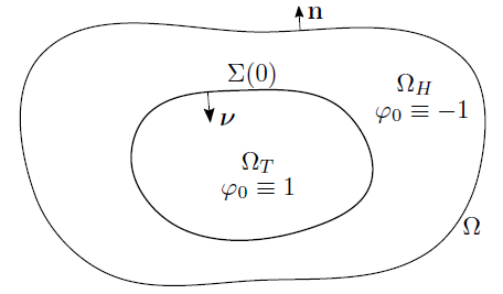
Since $\nabla\varphi_{0}=\mathbf{0}$ , $\partial_{t}\varphi_{0}=0$ in $\Omega_{T}$ and $\Omega_{H}$ , we obtain for the equations to zeroth order that


$\displaystyle\textnormal{div}(\mathbf{v}_{0})$	$\displaystyle=\tfrac{1}{\bar{\rho}_{2}}\Gamma_{2}(\varphi_{0},\sigma_{0},\mu_{0})+\tfrac{1}{\bar{\rho}_{1}}\Gamma_{1}(\varphi_{0},\sigma_{0},\mu_{0}),$	(4.4a)
$\displaystyle-\textnormal{div}(\mathbf{T}(\varphi_{0},\mathbf{v}_{0},p_{0}))+\nu(\varphi_{0})\mathbf{v}_{0}$	$\displaystyle=0,$	(4.4b)
$\displaystyle-\textnormal{div}(m(\varphi_{0})\nabla\mu_{0})$	$\displaystyle=\tfrac{1}{\bar{\rho}_{2}}\Gamma_{2}(\varphi_{0},\sigma_{0},\mu_{0})(1-\varphi_{0})$
	$\displaystyle\quad-\tfrac{1}{\bar{\rho}_{1}}\Gamma_{1}(\varphi_{0},\sigma_{0},\mu_{0})(1+\varphi_{0}),$	(4.4c)
$\displaystyle\partial_{t}\sigma_{0}+\textnormal{div}(\sigma_{0}\mathbf{v}_{0})$	$\displaystyle=\textnormal{div}(n(\varphi_{0})\chi_{\sigma}\nabla\sigma_{0})+\Gamma_{\sigma}(\varphi_{0},\sigma_{0},\mu_{0}),$	(4.4d)

where

\mathbf{T}(\varphi_{0},\mathbf{v}_{0},p_{0})=2\eta(\varphi_{0}){\mathbf{D}}\mathbf{v}_{0}+\lambda(\varphi_{0})\textnormal{div}(\mathbf{v}_{0})\mathbf{I}-p_{0}\mathbf{I}.

We now analyse the three different cases for (4.1c) according to the mobilities introduced in (4.2).
Case (i) ( $m(\varphi)=m_{0}$ ): In this case we obtain

	$-m_{0}\Delta\mu_{0}=\bar{\rho}_{2}^{-1}\Gamma_{2}(\varphi_{0},\sigma_{0},\mu_{0})(1-\varphi_{0})-\bar{\rho}_{1}^{-1}\Gamma_{1}(\varphi_{0},\sigma_{0},\mu_{0})(1+\varphi_{0}).$	(4.5a)
Case (ii) ( $m(\varphi)=\epsilon m_{0}$ ): The mobility is rescaled and the chemical potential does not contribute to the equations at zeroth order. Indeed, we have
	$\bar{\rho}_{2}^{-1}\Gamma_{2}(\varphi_{0},\sigma_{0},\mu_{0})(1-\varphi_{0})=\bar{\rho}_{1}^{-1}\Gamma_{1}(\varphi_{0},\sigma_{0},\mu_{0})(1+\varphi_{0}).$	(4.5b)
Case (iii) ( $m(\varphi)=\tfrac{m_{1}}{2}(1+\varphi)^{2}$ ): The degenerate mobility case leads to
	$-\textnormal{div}(\tfrac{m_{1}}{2}(1+\varphi_{0})^{2}\,\nabla\mu_{0})=\bar{\rho}_{2}^{-1}\Gamma_{2}(\varphi_{0},\sigma_{0},\mu_{0})(1-\varphi_{0})-\bar{\rho}_{1}^{-1}\Gamma_{1}(\varphi_{0},\sigma_{0},\mu_{0})(1+\varphi_{0}).$	(4.5c)

Remark 4.1.

(i)

In order to fulfil (4.5b) we have to assume that

\Gamma_{1}(1,\sigma_{0},\mu_{0})=0\quad\text{and}\quad\Gamma_{2}(-1,\sigma_{0},\mu_{0})=0.

(4.6)

Furthermore, we observe that for general source terms the chemical potential $\mu_{0}$ appears on the right hand side of (4.4a) although the bulk equations for $\mu_{0}$ remain undetermined. Therefore, it is reasonable to assume that the source terms are either independent of $\mu$ , i. e.,

\Gamma_{1}=\Gamma_{1}(\varphi,\sigma),\quad\Gamma_{2}=\Gamma_{2}(\varphi,\sigma),

(4.7)

or we may ask for

\Gamma_{1}(\pm 1,\sigma,\mu)=0,\quad\Gamma_{2}(\pm 1,\sigma,\mu)=0.

(4.8)

To fulfil (4.6) and (4.7) we could choose

\Gamma_{1}\equiv 0,\quad\Gamma_{2}(\varphi,\sigma)\coloneqq\frac{\bar{\rho}_{2}}{2}\left(\frac{1}{\bar{\rho}_{2}}-\frac{1}{\bar{\rho}_{1}}\right)(\mathcal{P}\sigma-\mathcal{A})(1+\varphi),

where $\mathcal{P}$ and $\mathcal{A}$ are non-negative constants related to proliferation and apoptosis, respectively. In this case the source terms in (4.1a), (4.1c) coincide and are of the form

\Gamma_{\varphi}(\varphi,\sigma)=\Gamma_{\mathbf{v}}(\varphi,\sigma)=\frac{\alpha}{2}(\mathcal{P}\sigma-\mathcal{A})(1+\varphi),

where

\alpha\coloneqq\frac{1}{\bar{\rho}_{2}}-\frac{1}{\bar{\rho}_{1}}.

Equation (4.6) can be interpreted as follows:

$\bullet$

in the pure tumour phases, there can be no growth of healthy cells,
$\bullet$

in regions of unmixed healthy tissue, there is no spontaneous growth of tumour cells.

In a situation where we assume no gain or loss of mass locally, i. e., $\Gamma_{2}=-\Gamma_{1}$ , condition (4.6) implies that

\Gamma_{1}(\pm 1,\sigma_{0},\mu_{0})=\Gamma_{2}(\pm 1,\sigma_{0},\mu_{0})=0,

which coincides with (4.8). Hence death and growth are restricted to the interfacial region and we may choose, for example,

\Gamma_{1}(\varphi,\sigma,\mu)=\gamma_{1}(\varphi,\sigma,\mu)(1-\varphi^{2})_{+}

for a function $\gamma_{1}$ to be specified. Alternatively we could use phenomenological laws to describe growth and death by choosing

\Gamma_{2}=-\Gamma_{1}=P_{1}(\varphi)(\chi_{\sigma}\sigma+\chi_{\varphi}(1-\varphi)-\mu),

where $P_{1}(\cdot)$ is a proliferation function satisfying $P_{1}(\pm 1)=0$ . For instance, we could take $P_{1}(\varphi)=\frac{1}{4}(1-\varphi^{2})^{2}$ .

(ii)

In the healthy region (4.5c) simplifies to

0=2\bar{\rho}_{2}^{-1}\Gamma_{2}(-1,\sigma_{0},\mu_{0}).

This is a compatibility for the source term $\Gamma_{2}$ . For similar reasons as before, we can assume that either the source terms are independent of $\mu$ or

\Gamma_{1}(-1,\sigma,\mu)=\Gamma_{2}(-1,\sigma,\mu)=0.

Reasonable choices are

\Gamma_{2}(\varphi,\sigma)=\gamma_{2}(\varphi,\sigma)(1+\varphi)_{+}

for some function $\gamma_{2}$ , or

\frac{\Gamma_{2}}{\bar{\rho}_{2}}=-\frac{\Gamma_{1}}{\bar{\rho}_{1}}=P_{2}(\varphi)(\chi_{\sigma}\sigma+\chi_{\varphi}(1-\varphi)-\mu),

where $P_{2}(\varphi)=p_{0}(1+\varphi)_{+}$ . This can be interpreted as a scaled zero excess of total mass and we have

\Gamma_{\varphi}=2P_{2}(\varphi)(\chi_{\sigma}\sigma+\chi_{\varphi}(1-\varphi)-\mu),\quad\Gamma_{\mathbf{v}}=0.

If the mobility was degenerate in both phases we would obtain the same condition as in (4.6).

(iii)

Similar conditions have to hold for the source term $\Gamma_{\sigma}$ . From now on we assume that the source terms are independent of $\mu$ .

4.2 Inner Expansion

4.2.1 New Coordinates and matching conditions

This subsection uses ideas presented in [1] and [41]. We denote by $\Sigma(0)$ the smooth evolving interface which is assumed to be the limit of the zero level sets $\Sigma(\epsilon)$ of $\varphi_{\epsilon}$ as $\epsilon\to 0$ (see, e. g., [41] for details). We now introduce new coordinates in a neighbourhood of $\Sigma(0)$ . To this end, we choose a time interval $I\subset\mathbb{R}$ and a spatial parameter domain $U\subset\mathbb{R}^{d-1}$ , and we define a local parametrisation of $\Sigma(0)$ by

\gamma\colon U\times I\to\mathbb{R}^{d}.

By $\bm{\nu}$ we denote the unit normal to $\Sigma(0)$ pointing into the tumour region. Close to $\gamma(U\times I)$ we consider the signed distance function $d(x,t)$ of a point $x$ to $\Sigma(0,t)$ with $d(x,t)>0$ if $x\in\Omega_{T}$ and $d(x,t)<0$ if $x\in\Omega_{H}$ . We introduce a local parametrisation of $\mathbb{R}^{d}\times I$ near $\gamma(U\times I)$ using the rescaled distance $z=\frac{d}{\epsilon}$ by

G^{\epsilon}(s,z,t)\coloneqq(\gamma(s,t)+\epsilon z\bm{\nu}(s,t),t)

with $s\in U\subset\mathbb{R}^{d-1}$ . We show a sketch of the situation in Figure 3.

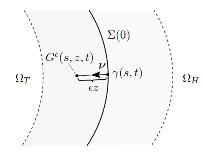
The (scalar) normal velocity is given by

\mathcal{V}=\partial_{t}\gamma\cdot\bm{\nu},

and we observe that $(G^{\epsilon})^{-1}(x,t)\eqqcolon(s,z,t)(x,t)$ fulfils

\partial_{t}z=\frac{1}{\epsilon}\partial_{t}d=-\frac{1}{\epsilon}\mathcal{V}.

In particular, it holds that $\bm{\nu}(x,t)=\nabla d(x,t)$ on $\Sigma(0,t)$ .
Let $b(x,t)$ be a scalar function and define $B(s(x,t),z(x,t),t)=b(x,t)$ . Then, in the new coordinate system, we obtain

\frac{\mathrm{d}}{\mathrm{d}t}b(x,t)=\partial_{t}B+\partial_{z}B\partial_{t}z+\nabla_{s}B\cdot\partial_{t}s=-\frac{1}{\epsilon}\mathcal{V}\partial_{z}B+\text{h.\,o.\,t.}\,.

For the gradient of $b$ we have

\nabla_{x}b=\nabla_{\Sigma_{\epsilon z}}B+\frac{1}{\epsilon}\partial_{z}B\bm{\nu},

where $\nabla_{\Sigma_{\epsilon z}}$ is the surface gradient on $\Sigma_{\epsilon z}\coloneqq\{\gamma(s)+\epsilon z\bm{\nu}\colon s\in U\}$ .
For a vector quantity $\mathbf{j}(x,t)=\mathbf{J}(s(x,t),z(x,t),t)$ we obtain

\nabla_{x}\cdot\mathbf{j}=\frac{1}{\epsilon}\partial_{z}\mathbf{J}\cdot\bm{\nu}+\textnormal{div}_{\Sigma_{\epsilon z}}\mathbf{J}

with $\textnormal{div}_{\Sigma_{\epsilon z}}$ being the surface divergence on $\Sigma_{\epsilon z}$ . Furthermore, it holds

\Delta_{x}b(x,t)=\frac{1}{\epsilon^{2}}\partial_{zz}B-\frac{1}{\epsilon}\kappa\partial_{z}B+\text{h.\,o.\,t.}\,,

where $\kappa$ is the mean curvature of $\Sigma(0)$ . In addition, we have

	$\displaystyle\nabla_{\Sigma_{\epsilon z}}B(s,z)$	$\displaystyle=\nabla_{\Sigma(0)}B(s,z)+\text{h.\,o.\,t.}\,,$
	$\displaystyle\textnormal{div}_{\Sigma_{\epsilon z}}\mathbf{J}(s,z)$	$\displaystyle=\textnormal{div}_{\Sigma(0)}\mathbf{J}(s,z)+\text{h.\,o.\,t.}\,,$
	$\displaystyle\Delta_{\Sigma_{\epsilon z}}B(s,z)$	$\displaystyle=\Delta_{\Sigma(0)}B(s,z)+\text{h.\,o.\,t.}\,.$

Summarising all the identities deduced so far yields


	$\displaystyle\frac{{\mathrm{d}}}{{\mathrm{d}}t}b(x,t)$	$\displaystyle=-\frac{1}{\epsilon}\mathcal{V}\partial_{z}B+\text{h.\,o.\,t.}\,,$	(4.9a)
	$\displaystyle\nabla_{x}b(x,t)$	$\displaystyle=\frac{1}{\epsilon}\partial_{z}B\bm{\nu}+\nabla_{\Sigma(0)}B+\text{h.\,o.\,t.}\,,$	(4.9b)
	$\displaystyle\Delta_{x}b(x,t)$	$\displaystyle=\frac{1}{\epsilon^{2}}\partial_{zz}B-\frac{1}{\epsilon}\kappa\partial_{z}B+\text{h.\,o.\,t.}\,,$	(4.9c)
	$\displaystyle\textnormal{div}_{x}\mathbf{j}(x,t)$	$\displaystyle=\frac{1}{\epsilon}\partial_{z}\mathbf{J}\cdot\bm{\nu}+\textnormal{div}_{\Sigma(0)}\mathbf{J}+\text{h.\,o.\,t.}\,.$	(4.9d)
Using (4.9b)-(4.9c) component-wise we obtain

	$\displaystyle\nabla_{x}\mathbf{j}$	$\displaystyle=\frac{1}{\epsilon}\partial_{z}\mathbf{J}\otimes\bm{\nu}+\nabla_{\Sigma(0)}\mathbf{J}+\text{h.\,o.\,t.}\,,$	(4.9e)
	$\displaystyle\Delta_{x}\mathbf{j}$	$\displaystyle=\frac{1}{\epsilon^{2}}\partial_{zz}\mathbf{J}-\frac{1}{\epsilon}\kappa\partial_{z}\mathbf{J}+\text{h.\,o.\,t.}\,.$	(4.9f)

We denote the variables $\varphi_{\epsilon}$ , $\mu_{\epsilon}$ , $\sigma_{\epsilon}$ , $\mathbf{v}_{\epsilon}$ , $p_{\epsilon}$ , in the new coordinate system by $\Phi_{\epsilon}$ , $\Xi_{\epsilon}$ , $C_{\epsilon}$ , $\mathbf{V}_{\epsilon}$ , $P_{\epsilon}$ , and we assume the following inner expansion

F_{\epsilon}(s,z)=F_{0}(s,z)+\epsilon F_{1}(s,z)+\epsilon^{2}F_{2}(s,z)+\dots

for $F_{\epsilon}\in\{\Phi_{\epsilon},\Xi_{\epsilon},C_{\epsilon},\mathbf{V}_{\epsilon},P_{\epsilon}\}$ . The assumption that the zero level sets of $\varphi_{\epsilon}$ converge to $\Sigma(0)$ implies

\Phi_{0}(s,z=0,t)=0.

We will employ the matching conditions (see [40])


$\displaystyle\lim_{z\to\pm\infty}F_{0}(s,z,t)$	$\displaystyle=f_{0}^{\pm}(x,t),$	(4.10a)
$\displaystyle\lim_{z\to\pm\infty}\partial_{z}F_{0}(s,z,t)$	$\displaystyle=0,$	(4.10b)
$\displaystyle\lim_{z\to\pm\infty}\partial_{z}F_{1}(s,z,t)$	$\displaystyle=\nabla f_{0}^{\pm}(x,t)\cdot\bm{\nu},$	(4.10c)

where

f_{0}^{\pm}(x,t)\coloneqq\lim_{\delta\searrow 0}f_{0}(x\pm\delta\bm{\nu},t)\quad\text{for }x\in\Sigma(0,t).

Moreover, we introduce the notation

[f]_{H}^{T}\coloneqq\lim_{\delta\searrow 0}f(x+\delta\bm{\nu},t)-\lim_{\delta\searrow 0}f(x-\delta\bm{\nu},t)\quad\text{for }x\in\Sigma(0,t)

to denote the jump of a quantity $f$ across the interface.

4.2.2 Inner Expansion to leading order

Step 1: From $\eqref{3_basic_equation_1d}_{I}^{-1}$ we obtain

\partial_{zz}\Phi_{0}-\psi^{\prime}(\Phi_{0})=0.

(4.11)

Since $\Phi_{0}(s,z=0,t)=0$ we can choose $\Phi_{0}$ independent of $s$ and $t$ , hence, $\Phi_{0}$ solves

\Phi_{0}^{\prime\prime}(z)-\psi^{\prime}(\Phi_{0}(z))=0,\quad\Phi_{0}(0)=0,\quad\Phi_{0}(\pm\infty)=\pm 1,

(4.12)

where we used (4.10a). The unique solution of (4.12) is given by

\Phi_{0}(z)=\tanh\left(\frac{z}{\sqrt{2}}\right).

This solution has the property of equipartition of energy

\frac{1}{2}|\Phi_{0}^{\prime}(z)|^{2}=\psi(\Phi_{0}(z))\quad\forall\,|z|<\infty.

(4.13)

Step 2: From $\eqref{3_basic_equation_1a}_{I}^{-1}$ we obtain (using (4.9d))

\partial_{z}\mathbf{V}_{0}\cdot\bm{\nu}=0.

(4.14)

Due to $\partial_{z}\bm{\nu}=\mathbf{0}$ this implies

\partial_{z}(\mathbf{V}_{0}\cdot\bm{\nu})=0.

(4.15)

Integrating this identity gives

0=\int_{-\infty}^{\infty}\partial_{z}(\mathbf{V}_{0}\cdot\bm{\nu})\;\mathrm{d}z=[\mathbf{V}_{0}\cdot\bm{\nu}]_{-\infty}^{\infty}.

Hence, the matching condition (4.10a) yields

[\mathbf{v}_{0}]_{H}^{T}\cdot\bm{\nu}\coloneqq\mathbf{v}_{0}^{+}\cdot\bm{\nu}-\mathbf{v}_{0}^{-}\cdot\bm{\nu}=0.

(4.16)

Step 3: We now analyse (4.1c). The terms $\bar{\rho}_{2}^{-1}\Gamma_{2}$ and $\bar{\rho}_{1}^{-1}\Gamma_{1}$ do not contribute to leading order. We distinguish again the three cases for the mobilities:
Case (i) ( $m(\varphi)=m_{0}$ ): Using (4.9), from $\eqref{3_basic_equation_1c}_{I}^{-2}$ we get

m_{0}\partial_{zz}\Xi_{0}=0.

Upon integrating and using the matching condition (4.10b) we obtain

\partial_{z}\Xi_{0}=0\quad\forall\,|z|<\infty.

Integrating again from $-\infty$ to $\infty$ and using the matching condition (4.10a), yields

[\mu_{0}]_{H}^{T}=0.

Case (ii) ( $m(\varphi)=\epsilon m_{0}$ ): Using (4.9) we obtain from $\eqref{3_basic_equation_1c}_{I}^{-1}$ that

-\mathcal{V}\Phi_{0}^{\prime}+\partial_{z}(\Phi_{0}\mathbf{V}_{0})\cdot\bm{\nu}=\partial_{z}(m_{0}\partial_{z}\Xi_{0}).

(4.17)

Integrating this identity and using $\partial_{z}\mathcal{V}=0$ , $\partial_{z}\bm{\nu}=\mathbf{0}$ in conjunction with (4.15) and (4.10b) gives

2(-\mathcal{V}+\mathbf{v}_{0}\cdot\bm{\nu})=0.

In particular, we obtain from (4.15)-(4.16) and (4.17) that

m_{0}\partial_{zz}\Xi_{0}=(-\mathcal{V}+\mathbf{v}_{0}\cdot\bm{\nu})\Phi_{0}^{\prime}=0,

which together with the matching condition (4.10b) implies that $\partial_{z}\Xi_{0}=0$ for all $|z|<\infty$ . Hence, we obtain that $\Xi_{0}$ is independent of $z$ .
Case (iii) $\big(m(\varphi)=\tfrac{m_{1}}{2}(1+\varphi)^{2}\big)$ : With similar arguments as above we obtain from $\eqref{3_basic_equation_1c}_{I}^{-2}$ that

\tfrac{m_{1}}{2}\partial_{z}((1+\Phi_{0})^{2}\,\partial_{z}\Xi_{0})=0.

Integrating this inequality in time from $-\infty$ to $z$ with $|z|<\infty$ and using the matching condition (4.10b) gives

\tfrac{m_{1}}{2}(1+\Phi_{0})^{2}\partial_{z}\Xi_{0}(s,z,t)=0\quad\forall\,|z|<\infty.

Since $|\Phi_{0}(z)|<1$ for $|z|<\infty$ , this implies that

\partial_{z}\Xi_{0}(s,z,t)=0\quad\forall\,|z|<\infty,

and therefore $\Xi_{0}$ is independent of $z$ .
Step 4: Using $\partial_{z}\bm{\nu}=\mathbf{0}$ and applying similar calculations as for (4.1c), from $\eqref{3_basic_equation_1e}_{I}^{-2}$ we obtain

\partial_{z}(n(\Phi_{0})\chi_{\sigma}\partial_{z}C_{0})-\partial_{z}(n(\Phi_{0})\chi_{\varphi}\partial_{z}\Phi_{0})=0.

Integrating this identity from $-\infty$ to $z$ with $|z|<\infty$ and using (4.10b) yields

n(\Phi_{0})(\chi_{\sigma}\partial_{z}C_{0}-\chi_{\varphi}\Phi_{0}^{\prime}(z))=0\quad\forall\,|z|<\infty.

Since $n(\Phi_{0})>0$ , this means

\chi_{\sigma}\partial_{z}C_{0}(s,z,t)=\chi_{\varphi}\Phi_{0}^{\prime}(z)\quad\forall\,|z|<\infty.

(4.18)

Upon integrating and using (4.10a) we see that

[\sigma_{0}]_{H}^{T}=[C_{0}(s,z,t)]_{-\infty}^{+\infty}=\int_{-\infty}^{\infty}\partial_{z}C_{0}(s,z,t)\;\mathrm{d}z=\frac{\chi_{\varphi}}{\chi_{\sigma}}\int_{-\infty}^{\infty}\Phi_{0}^{\prime}(z)\;\mathrm{d}z=2\frac{\chi_{\varphi}}{\chi_{\sigma}}.

Step 5: Finally, we analyse (4.1b) and we define $\mathcal{E}(\mathbf{A})=\frac{1}{2}(\mathbf{A}+\mathbf{A}^{\intercal})$ for a square matrix $\mathbf{A}$ . Using (4.9b), (4.9e) and (4.14), with similar arguments as in [1] we obtain from $\eqref{3_basic_equation_1b}_{I}^{-2}$ that

\partial_{z}(2\eta(\Phi_{0})\mathcal{E}(\partial_{z}\mathbf{V}_{0}\otimes\bm{\nu})\bm{\nu})=\mathbf{0}.

(4.19)

Due to (4.15) we have

(\bm{\nu}\otimes\partial_{z}\mathbf{V}_{0})\bm{\nu}=(\partial_{z}\mathbf{V}_{0}\cdot\bm{\nu})\bm{\nu}=\mathbf{0}.

Together with (4.19) and the identity $(\partial_{z}\mathbf{V}_{0}\otimes\bm{\nu})\bm{\nu}=\partial_{z}\mathbf{V}_{0}$ , this implies

\partial_{z}(\eta(\Phi_{0})\partial_{z}\mathbf{V}_{0})=\mathbf{0}.

Integrating from $-\infty$ to $z$ with $|z|<\infty$ , using the matching condition (4.10b) and the positivity of $\eta(\cdot)$ , this gives

\partial_{z}\mathbf{V}_{0}=\mathbf{0}\quad\forall\,|z|<\infty.

(4.20)

Once more integrating and using the matching condition (4.10a) yields

[\mathbf{v}_{0}]_{H}^{T}=\mathbf{0}.

(4.21)

4.2.3 Inner Expansion to higher order

We will now expand the equations in the inner regions to the next highest order.
Step 1: From $\eqref{3_basic_equation_1d}_{I}^{0}$ , we obtain

\beta\Phi_{1}\psi^{\prime\prime}(\Phi_{0})+\beta\kappa\Phi_{0}^{\prime}-\beta\partial_{zz}\Phi_{1}-\chi_{\varphi}C_{0}=\Xi_{0}.

Multiplying by $\Phi_{0}^{\prime}$ and integrating from $-\infty$ to $+\infty$ yields

\int_{-\infty}^{\infty}\Xi_{0}(s,t)\Phi_{0}^{\prime}(z)\;\mathrm{d}z=\int_{-\infty}^{\infty}\beta(\psi^{\prime}(\Phi_{0}))^{\prime}\Phi_{1}-\beta\partial_{zz}\Phi_{1}\Phi_{0}^{\prime}+\beta\kappa|\Phi_{0}^{\prime}|^{2}-\chi_{\varphi}C_{0}\Phi_{0}^{\prime}\;\mathrm{d}z.

(4.22)

Using (4.10a)-(4.10b), (4.11) and $\psi^{\prime}(\pm 1)=0$ , integration by parts gives

	$\displaystyle\int_{-\infty}^{\infty}(\psi^{\prime}(\Phi_{0}))^{\prime}\Phi_{1}-\partial_{zz}\Phi_{1}\Phi_{0}^{\prime}{\mathrm{d}}z$	$\displaystyle=[\psi^{\prime}(\Phi_{0})\Phi_{1}-\partial_{z}\Phi_{1}\Phi_{0}^{\prime}]_{-\infty}^{+\infty}$
		$\displaystyle\quad-\int_{-\infty}^{\infty}\partial_{z}\Phi_{1}(\psi^{\prime}(\Phi_{0})-\Phi_{0}^{\prime\prime})\;\mathrm{d}z=0.$		(4.23)

Recalling that $\Xi_{0}$ is independent of $z$ and applying the matching condition (4.10a) we have

\int_{-\infty}^{+\infty}\Xi_{0}(s,t)\Phi_{0}^{\prime}(z)\;\mathrm{d}z=2\mu_{0}.

(4.24)

By the equipartition of energy (4.13) we compute

	$\displaystyle\int_{-\infty}^{\infty}\|\Phi_{0}^{\prime}(z)\|^{2}\;\mathrm{d}z$	$\displaystyle=\int_{-\infty}^{\infty}\|\Phi_{0}^{\prime}(z)\|\sqrt{2\psi(\Phi_{0}(z))}\;\mathrm{d}z=\int_{-1}^{1}\sqrt{2\psi(y)}\;\mathrm{d}y$
		$\displaystyle=\frac{1}{\sqrt{2}}\int_{-1}^{1}(1-y^{2})\;\mathrm{d}y=\frac{2\sqrt{2}}{2}\eqqcolon\tau,$

and obtain

\int_{-\infty}^{+\infty}\beta\kappa|\Phi_{0}^{\prime}(z)|^{2}\;\mathrm{d}z=\beta\kappa\tau.

(4.25)

Finally, by (4.18) we obtain

	$\displaystyle\int_{-\infty}^{+\infty}\chi_{\varphi}C_{0}\Phi_{0}^{\prime}(z)\;\mathrm{d}z=\chi_{\sigma}\int_{-\infty}^{+\infty}\partial_{z}C_{0}(s,z,t)C_{0}(s,z,t)\;\mathrm{d}z$	$\displaystyle=\frac{\chi_{\sigma}}{2}\int_{-\infty}^{+\infty}\partial_{z}(\|C_{0}\|^{2})\;\mathrm{d}z$
		$\displaystyle=\frac{\chi_{\sigma}}{2}[\|\sigma_{0}\|^{2}]_{H}^{T}.$		(4.26)

Collecting (4.22)-(4.26) gives

2\mu_{0}=\beta\kappa\tau-\frac{\chi_{\sigma}}{2}[|\sigma_{0}|^{2}]_{H}^{T}.

(4.27)

This is a solvability condition for $\Phi_{1}$ , the so-called Gibbs–Thomas equation.
Step 2: With similar arguments as above and using (4.18), equation $\eqref{3_basic_equation_1e}_{I}^{-1}$ gives

(-\mathcal{V}+\mathbf{V}_{0}\cdot\bm{\nu})\partial_{z}C_{0}=\partial_{z}(n(\Phi_{0})(\chi_{\sigma}\partial_{z}C_{1}-\chi_{\varphi}\partial_{z}\Phi_{1})).

Employing the matching condition (4.10c) and $\nabla\varphi_{0}=\mathbf{0}$ in the bulk regions together with $\partial_{z}\mathcal{V}=0$ and (4.15), this yields

	$\displaystyle(-\mathcal{V}+\mathbf{v}_{0}\cdot\bm{\nu})[\sigma_{0}]_{H}^{T}$	$\displaystyle=\int_{-\infty}^{\infty}(-\mathcal{V}+\mathbf{V}_{0}\cdot\bm{\nu})\partial_{z}C_{0}\;\mathrm{d}z$
		$\displaystyle=\int_{-\infty}^{+\infty}\partial_{z}(n(\Phi_{0})(\chi_{\sigma}\partial_{z}C_{1}-\chi_{\varphi}\partial_{z}\Phi_{1}))\;\mathrm{d}z=\chi_{\sigma}[n(\varphi_{0})\nabla\sigma_{0}]_{H}^{T}\cdot\bm{\nu}.$

Step 3: Similar as in [1] we analyse (4.1c) only for the mobilities (4.2)(i) and (iii) since the case (4.2)(ii) is rescaled and therefore does not contribute to the sharp interface limit.
Case (i) ( $m(\varphi)=m_{0}$ ): Using $\partial_{z}\Xi_{0}=0$ and (4.14), from $\eqref{3_basic_equation_1c}_{I}^{-1}$ we obtain

(-\mathcal{V}+\mathbf{V}_{0}\cdot\bm{\nu})\Phi_{0}^{\prime}=m_{0}\partial_{zz}\Xi_{1}.

Integrating with respect to $z$ from $-\infty$ to $\infty$ , using (4.15)-(4.16) and the matching condition (4.10c), this yields

2(-\mathcal{V}+\mathbf{v}_{0}\cdot\bm{\nu})=m_{0}[\nabla\mu_{0}]_{H}^{T}\cdot\bm{\nu}.

(4.28)

Case (iii) $\big(m(\varphi)=m_{1}(1+\varphi)^{2}\big)$ : With similar arguments as above we obtain

(-\mathcal{V}+\mathbf{V}_{0}\cdot\bm{\nu})\Phi_{0}^{\prime}=\tfrac{m_{1}}{2}\partial_{z}\left((1+\Phi_{0})^{2}\partial_{z}\Xi_{1}\right).

Using the matching conditions (4.10a), (4.10c) and the same arguments as for (4.28), this entails

(-\mathcal{V}+\mathbf{v}_{0}\cdot\bm{\nu})=m_{1}\nabla\mu_{0}^{T}\cdot\bm{\nu}.

Step 4: Finally, we consider the momentum balance equation (4.1b) at order $\epsilon^{-1}$ . Using (4.9) and (4.20), with similar arguments as above we obtain from $\eqref{3_basic_equation_1b}_{I}^{-1}$

		$\displaystyle-\partial_{z}\big(2\eta(\Phi_{0})\mathcal{E}(\partial_{z}\mathbf{V}_{1}\otimes\bm{\nu})\bm{\nu}+2\eta(\Phi_{0})\mathcal{E}(\nabla_{\Sigma(0)}\mathbf{V}_{0})\bm{\nu}\big)$
		$\displaystyle\qquad-\partial_{z}\big(\lambda(\Phi_{0})(\partial_{z}\mathbf{V}_{1}\cdot\bm{\nu}+\textnormal{div}_{\Sigma(0)}\mathbf{V}_{0})\bm{\nu}-P_{0}\bm{\nu}\big)$
		$\displaystyle\quad=(\Xi_{0}+\chi_{\varphi}C_{0})\Phi_{0}^{\prime}\bm{\nu}.$		(4.29)

Since matching requires $\lim_{z\to\pm\infty}\partial_{z}\mathbf{V}_{1}(z)=(\nabla\mathbf{v}_{0}^{\pm})\bm{\nu}$ , we conclude

	$\displaystyle(\partial_{z}\mathbf{V}_{1}\otimes\bm{\nu}+\nabla_{\Sigma(0)}\mathbf{V}_{0})$	$\displaystyle\to\nabla_{x}\mathbf{v}_{0}$		$\displaystyle\quad\text{for}\quad z\to\pm\infty,$
	$\displaystyle(\partial_{z}\mathbf{V}_{1}\cdot\bm{\nu}+\textnormal{div}_{\Sigma(0)}\mathbf{V}_{0})$	$\displaystyle\to\textnormal{div}_{x}\mathbf{v}_{0}$		$\displaystyle\quad\text{for}\quad z\to\pm\infty.$

Integrating (4.29) with respect to $z$ from $-\infty$ to $+\infty$ and using (4.10a), this implies

		$\displaystyle-[2\eta(\varphi_{0})\mathcal{E}(\nabla_{x}\mathbf{v}_{0})+\lambda(\varphi_{0})\textnormal{div}(\mathbf{v}_{0})\mathbf{I}-p_{0}\mathbf{I}]_{H}^{T}\bm{\nu}$
		$\displaystyle\qquad=\int_{-\infty}^{+\infty}(\Xi_{0}(s,t)+\chi_{\varphi}C_{0}(s,z,t))\Phi_{0}^{\prime}(z)\bm{\nu}\;\mathrm{d}z.$

Together with (4.24) and (4.26)-(4.27), we end up at

[\mathbf{T}(\varphi_{0},\mathbf{v}_{0},p_{0})]_{H}^{T}\bm{\nu}=-\beta\kappa\tau\bm{\nu}.

4.3 Equations of the formal sharp interface limit

For the reader’s convenience, we summarise the sharp interface models for the different mobilities:
Case (i) ( $m(\varphi)=m_{0}$ ) The equations in the bulk are given by

$\displaystyle-\textnormal{div}(\mathbf{T}(\varphi_{0},\mathbf{v}_{0},p_{0}))+\nu(\varphi_{0})\mathbf{v}_{0}$	$\displaystyle=0$	$\displaystyle\qquad\text{in }\Omega_{T}\cup\Omega_{H},$
$\displaystyle\textnormal{div}(\mathbf{v}_{0}^{T})$	$\displaystyle=\bar{\rho}_{2}^{-1}\Gamma_{2}(1,\sigma_{0}^{T})+\bar{\rho}_{1}^{-1}\Gamma_{1}(1,\sigma_{0}^{T})$	$\displaystyle\qquad\text{in }\Omega_{T},$
$\displaystyle\textnormal{div}(\mathbf{v}_{0}^{H})$	$\displaystyle=\bar{\rho}_{2}^{-1}\Gamma_{2}(-1,\sigma_{0}^{H})+\bar{\rho}_{1}^{-1}\Gamma_{1}(-1,\sigma_{0}^{H})$	$\displaystyle\qquad\text{in }\Omega_{H},$
$\displaystyle-m_{0}\Delta\mu_{0}^{T}$	$\displaystyle=-2\bar{\rho}_{1}^{-1}\Gamma_{1}(1,\sigma_{0}^{T})$	$\displaystyle\qquad\text{in }\Omega_{T},$
$\displaystyle-m_{0}\Delta\mu_{0}^{H}$	$\displaystyle=2\bar{\rho}_{2}^{-1}\Gamma_{2}(-1,\sigma_{0}^{H})$	$\displaystyle\qquad\text{in }\Omega_{H},$
$\displaystyle\partial_{t}\sigma_{0}^{T}+\textnormal{div}(\sigma_{0}^{T}\mathbf{v}_{0}^{T})$	$\displaystyle=\textnormal{div}(n(1)\chi_{\sigma}\nabla\sigma_{0}^{T})-\Gamma_{\sigma}(1,\sigma_{0}^{T})$	$\displaystyle\qquad\text{in }\Omega_{T},$
$\displaystyle\partial_{t}\sigma_{0}^{H}+\textnormal{div}(\sigma_{0}^{H}\mathbf{v}_{0}^{H})$	$\displaystyle=\textnormal{div}(n(-1)\chi_{\sigma}\nabla\sigma_{0}^{H})-\Gamma_{\sigma}(-1,\sigma_{0}^{H})$	$\displaystyle\qquad\text{in }\Omega_{H}.$

Furthermore, on $\Sigma(0)$ we have the free boundary conditions

		$\displaystyle[\mathbf{v}_{0}]_{H}^{T}=\mathbf{0},\qquad[\mu_{0}]_{H}^{T}=0,\qquad[\sigma_{0}]_{H}^{T}=2\tfrac{\chi_{\varphi}}{\chi_{\sigma}},$
		$\displaystyle 2\mu_{0}=\beta\kappa\tau-\tfrac{\chi_{\sigma}}{2}[\|\sigma_{0}\|^{2}]_{H}^{T},\qquad(-\mathcal{V}+\mathbf{v}_{0}\cdot\bm{\nu})[\sigma_{0}]_{H}^{T}=[n(\varphi_{0})\nabla\sigma_{0}]_{H}^{T}\cdot\bm{\nu},$
		$\displaystyle 2(-\mathcal{V}+\mathbf{v}_{0}\cdot\bm{\nu})=m_{0}[\nabla\mu_{0}]_{H}^{T}\cdot\bm{\nu},\qquad[\mathbf{T}(\varphi_{0},\mathbf{v}_{0},p_{0})]_{H}^{T}\bm{\nu}=-\beta\kappa\tau\bm{\nu}.$

Case (ii) ( $m(\varphi)=\epsilon m_{0}$ ) The equations in the bulk are given by

$\displaystyle-\textnormal{div}(\mathbf{T}(\varphi_{0},\mathbf{v}_{0},p_{0}))+\nu(\varphi_{0})\mathbf{v}_{0}$	$\displaystyle=0$	$\displaystyle\qquad\text{in }\Omega_{T}\cup\Omega_{H},$
$\displaystyle\textnormal{div}(\mathbf{v}_{0}^{T})$	$\displaystyle=\bar{\rho}_{2}^{-1}\Gamma_{2}(1,\sigma_{0}^{T})$	$\displaystyle\qquad\text{in }\Omega_{T},$
$\displaystyle\textnormal{div}(\mathbf{v}_{0}^{H})$	$\displaystyle=\bar{\rho}_{1}^{-1}\Gamma_{1}(-1,\sigma_{0}^{H})$	$\displaystyle\qquad\text{in }\Omega_{H},$
$\displaystyle\partial_{t}\sigma_{0}^{T}+\textnormal{div}(\sigma_{0}^{T}\mathbf{v}_{0}^{T})$	$\displaystyle=\textnormal{div}(n(1)\chi_{\sigma}\nabla\sigma_{0}^{T})-\Gamma_{\sigma}(1,\sigma_{0}^{T})$	$\displaystyle\qquad\text{in }\Omega_{T},$
$\displaystyle\partial_{t}\sigma_{0}^{H}+\textnormal{div}(\sigma_{0}^{H}\mathbf{v}_{0}^{H})$	$\displaystyle=\textnormal{div}(n(-1)\chi_{\sigma}\nabla\sigma_{0}^{H})-\Gamma_{\sigma}(-1,\sigma_{0}^{H})$	$\displaystyle\qquad\text{in }\Omega_{H}.$

Furthermore, on $\Sigma(0)$ we have the free boundary conditions

		$\displaystyle[\mathbf{v}_{0}]_{H}^{T}=\mathbf{0},\qquad[\sigma_{0}]_{H}^{T}=2\tfrac{\chi_{\varphi}}{\chi_{\sigma}},\qquad 0=[n(\varphi_{0})\nabla\sigma_{0}]_{H}^{T}\cdot\bm{\nu},$
		$\displaystyle\mathcal{V}=\mathbf{v}_{0}\cdot\bm{\nu},\qquad[\mathbf{T}(\varphi_{0},\mathbf{v}_{0},p_{0})]_{H}^{T}\bm{\nu}=-\beta\kappa\tau\bm{\nu}.$

Case (iii) $\big(m(\varphi)=m_{1}(1+\varphi)^{2}\big)$ The equations in the bulk are given by

$\displaystyle-\textnormal{div}(\mathbf{T}(\varphi_{0},\mathbf{v}_{0},p_{0}))+\nu(\varphi_{0})\mathbf{v}_{0}$	$\displaystyle=0$	$\displaystyle\qquad\text{in }\Omega_{T}\cup\Omega_{H},$
$\displaystyle\textnormal{div}(\mathbf{v}_{0}^{T})$	$\displaystyle=\bar{\rho}_{2}^{-1}\Gamma_{2}(1,\sigma_{0}^{T})+\bar{\rho}_{1}^{-1}\Gamma_{1}(1,\sigma_{0}^{T})$	$\displaystyle\qquad\text{in }\Omega_{T},$
$\displaystyle\textnormal{div}(\mathbf{v}_{0}^{H})$	$\displaystyle=\bar{\rho}_{1}^{-1}\Gamma_{1}(-1,\sigma_{0}^{H})$	$\displaystyle\qquad\text{in }\Omega_{H},$
$\displaystyle-m_{1}\Delta\mu_{0}^{T}$	$\displaystyle=-\bar{\rho}_{1}^{-1}\Gamma_{1}(1,\sigma_{0}^{T})$	$\displaystyle\qquad\text{in }\Omega_{T},$
$\displaystyle\partial_{t}\sigma_{0}^{T}+\textnormal{div}(\sigma_{0}^{T}\mathbf{v}_{0}^{T})$	$\displaystyle=\textnormal{div}(n(1)\chi_{\sigma}\nabla\sigma_{0}^{T})-\Gamma_{\sigma}(1,\sigma_{0}^{T})$	$\displaystyle\qquad\text{in }\Omega_{T},$
$\displaystyle\partial_{t}\sigma_{0}^{H}+\textnormal{div}(\sigma_{0}^{H}\mathbf{v}_{0}^{H})$	$\displaystyle=\textnormal{div}(n(-1)\chi_{\sigma}\nabla\sigma_{0}^{H})-\Gamma_{\sigma}(-1,\sigma_{0}^{H})$	$\displaystyle\qquad\text{in }\Omega_{H}.$

Furthermore, on $\Sigma(0)$ we have the free boundary conditions

		$\displaystyle[\mathbf{v}_{0}]_{H}^{T}=\mathbf{0},\qquad[\sigma_{0}]_{H}^{T}=2\tfrac{\chi_{\varphi}}{\chi_{\sigma}},\qquad 2\mu_{0}=\beta\kappa\tau-\tfrac{\chi_{\sigma}}{2}[\|\sigma_{0}\|^{2}]_{H}^{T},$
		$\displaystyle(-\mathcal{V}+\mathbf{v}_{0}\cdot\bm{\nu})[\sigma_{0}]_{H}^{T}=[n(\varphi_{0})\nabla\sigma_{0}]_{H}^{T}\cdot\bm{\nu},\qquad(-\mathcal{V}+\mathbf{v}_{0}\cdot\bm{\nu})=m_{1}\nabla\mu_{0}^{T}\cdot\bm{\nu},$
		$\displaystyle[\mathbf{T}(\varphi_{0},\mathbf{v}_{0},p_{0})]_{H}^{T}\bm{\nu}=-\beta\kappa\tau\bm{\nu}.$

4.4 Specific sharp interface models

4.4.1 The limit of vanishing active transport, Darcy’s law and Stokes’ flow

We consider (4.1a)-(4.1e) with quasi-static nutrients and the mobility (4.2)(ii) along with constant viscosities and permeability. Moreover, we decouple chemotaxis and active transport according to (3.6), and we set

\mathcal{D}(\varphi)=\frac{1+\varphi}{2}+\mathcal{D}\frac{1-\varphi}{2}

for a constant $\mathcal{D}>0$ . Moreover, we choose

\Gamma_{1}\equiv 0,\qquad\Gamma_{2}(\varphi,\sigma)=\frac{\bar{\rho}_{2}}{2}\left(\frac{1}{\bar{\rho}_{2}}-\frac{1}{\bar{\rho}_{1}}\right)(\mathcal{P}\sigma-\mathcal{A})(1+\varphi),\qquad\Gamma_{\sigma}(\varphi,\sigma)=\frac{\mathcal{C}}{2}\sigma(1+\varphi).

This gives the following system of equations

	$\displaystyle\textnormal{div}(\mathbf{v})$	$\displaystyle=\frac{\alpha}{2}(\mathcal{P}\sigma-\mathcal{A})(1+\varphi),$
	$\displaystyle-\textnormal{div}(\mathbf{T}(\mathbf{v},p))+\nu\mathbf{v}$	$\displaystyle=(\mu+\chi_{\varphi}\sigma)\nabla\varphi,$
	$\displaystyle\partial_{t}\varphi+\nabla\varphi\cdot\mathbf{v}$	$\displaystyle=\textnormal{div}(\epsilon m_{0}\nabla\mu)+\frac{\alpha}{2}(\mathcal{P}\sigma-\mathcal{A})(1-\varphi^{2}),$
	$\displaystyle\mu$	$\displaystyle=\tfrac{\beta}{\epsilon}\psi^{\prime}(\varphi)-\beta\epsilon\Delta\varphi-\chi_{\varphi}\sigma,$
	$\displaystyle 0$	$\displaystyle=\textnormal{div}(\mathcal{D}(\varphi)\nabla\sigma)-\chi\textnormal{div}(\mathcal{D}(\varphi)\nabla\varphi)-\mathcal{C}\sigma(1+\varphi),$

where $\mathbf{T}(\mathbf{v},p)=2\eta{\mathbf{D}}\mathbf{v}+\lambda\textnormal{div}(\mathbf{v})\mathbf{I}-p\mathbf{I}$ . With slightly different arguments as above (see also [40]) and sending $\chi\to 0$ , we obtain


	$\displaystyle-\textnormal{div}(\mathbf{T}(\mathbf{v}_{0},p_{0}))+\nu\mathbf{v}_{0}$	$\displaystyle=0\qquad\text{in }\Omega_{T}\cup\Omega_{H},$	(4.30a)
	$\displaystyle\textnormal{div}(\mathbf{v}_{0})$	$\displaystyle=\begin{cases}\alpha(\mathcal{P}\sigma_{0}^{T}-\mathcal{A})&\text{in }\Omega_{T},\\ 0&\text{in }\Omega_{H},\end{cases}$	(4.30b)
	$\displaystyle\Delta\sigma_{0}$	$\displaystyle=\begin{cases}\mathcal{C}\sigma_{0}&\text{in }\Omega_{T},\\ 0&\text{in }\Omega_{H},\end{cases}$	(4.30c)
and the free boundary conditions on $\Sigma(0)$ are given by

		$\displaystyle[\mathbf{v}_{0}]_{H}^{T}=\mathbf{0},\qquad[\sigma_{0}]_{H}^{T}=0,\qquad\nabla\sigma_{0}^{T}\cdot\bm{\nu}=\mathcal{D}\nabla\sigma_{0}^{H}\cdot\bm{\nu},$	(4.30d)
		$\displaystyle\mathcal{V}=\mathbf{v}_{0}\cdot\bm{\nu},\qquad[\mathbf{T}(\mathbf{v}_{0},p_{0})]_{H}^{T}\bm{\nu}=-\beta\kappa\tau\bm{\nu}.$	(4.30d)

This model is a special case of the two-phase free boundary problem in [64], where numerical simulations for (4.30) are presented. Similar models have been studied in [17]. For a one-phase model with Brinkman’s law for the velocity we refer to [56].
Sending the viscosities to $0$ in (4.30), we can express the velocity in terms of the pressure and we obtain the following Darcy-type model

	$\displaystyle-\Delta p_{0}$	$\displaystyle=\begin{cases}\nu\,\alpha(\mathcal{P}\sigma_{0}^{T}-\mathcal{A})&\text{in }\Omega_{T},\\ 0&\text{in }\Omega_{H},\end{cases}$
	$\displaystyle\Delta\sigma_{0}$	$\displaystyle=\begin{cases}\mathcal{C}\sigma_{0}&\text{in }\Omega_{T},\\ 0&\text{in }\Omega_{H},\end{cases}$

where the free boundary conditions on $\Sigma(0)$ are given by

[\sigma_{0}]_{H}^{T}=0,\ \nabla\sigma_{0}^{T}\cdot\bm{\nu}=\mathcal{D}\nabla\sigma_{0}^{H}\cdot\bm{\nu},\ \tfrac{1}{\nu}[\nabla p_{0}]_{H}^{T}\cdot\bm{\nu}=0,\ \mathcal{V}=-\tfrac{1}{\nu}\nabla p_{0}\cdot\bm{\nu},\ [p_{0}]_{H}^{T}=-\beta\kappa\tau.

Similar models have been studied in, e. g., [15, 43, 52, 53]. We remark that the continuity condition for $\mathbf{v}_{0}$ across the interface (see (4.21)) is based on the positivity of the shear viscosity.
Sending the permeability to zero in (4.30), i. e., $\nu\to 0$ , we obtain a Stokes model given by

	$\displaystyle-\textnormal{div}(2\eta{\mathbf{D}}\mathbf{v}_{0}+\lambda\textnormal{div}(\mathbf{v}_{0})\mathbf{I}-p_{0}\mathbf{I})$	$\displaystyle=0\qquad\text{in }\Omega_{T}\cup\Omega_{H},$
	$\displaystyle\textnormal{div}(\mathbf{v}_{0})$	$\displaystyle=\begin{cases}\alpha(\mathcal{P}\sigma_{0}^{T}-\mathcal{A})&\text{in }\Omega_{T},\\ 0&\text{in }\Omega_{H},\end{cases}$
	$\displaystyle\Delta\sigma_{0}$	$\displaystyle=\begin{cases}\mathcal{C}\sigma_{0}&\text{in }\Omega_{T},\\ 0&\text{in }\Omega_{H},\end{cases}$

and the free boundary conditions on $\Sigma(0)$ are given by

		$\displaystyle[\mathbf{v}_{0}]_{H}^{T}=\mathbf{0},\qquad[\sigma_{0}]_{H}^{T}=0,\qquad\nabla\sigma_{0}^{T}\cdot\bm{\nu}=\mathcal{D}\nabla\sigma_{0}^{H}\cdot\bm{\nu},$
		$\displaystyle\mathcal{V}=\mathbf{v}_{0}\cdot\bm{\nu},\qquad[2\eta{\mathbf{D}}\mathbf{v}_{0}+\lambda\textnormal{div}(\mathbf{v}_{0})\mathbf{I}-p_{0}\mathbf{I}]_{H}^{T}\bm{\nu}=-\beta\kappa\tau\bm{\nu}.$

For similar models, we refer to [26, 27, 29, 30, 31, 32, 63].
We remark that a similar asymptotic analysis can be performed for the double obstacle potential

\psi(\varphi)\coloneqq\frac{1}{2}(1-\varphi^{2})+I_{[-1,1]}(\varphi),\quad I_{[-1,1]}(\varphi)=\begin{cases}0&\text{if }|\varphi|\leq 1,\\ +\infty&\text{elsewhere}.\end{cases}

(4.31)

To do so one combines the arguments above with the asymptotic analysis in [40]. We refer to [20] for details.

5 Analytical results

Our aim is to analyse the following variant of (2.21)


$\displaystyle\textnormal{div}(\mathbf{v})$	$\displaystyle=0$	$\displaystyle\qquad\text{ in }Q,$	(5.1a)
$\displaystyle-\textnormal{div}(2\eta{\mathbf{D}}\mathbf{v})+\nu\mathbf{v}-\nabla p$	$\displaystyle=-\epsilon\,\textnormal{div}(\nabla\varphi\otimes\nabla\varphi)$	$\displaystyle\qquad\text{ in }Q,$	(5.1b)
$\displaystyle\partial_{t}\varphi+\textnormal{div}(\varphi\mathbf{v})$	$\displaystyle=\textnormal{div}(m(\varphi)\nabla\mu)+g(\varphi,\sigma)h(\varphi)$	$\displaystyle\qquad\text{ in }Q,$	(5.1c)
$\displaystyle\mu$	$\displaystyle=-\epsilon\Delta\varphi+\epsilon^{-1}\psi^{\prime}(\varphi)-\chi_{\varphi}\sigma$	$\displaystyle\qquad\text{ in }Q,$	(5.1d)
$\displaystyle\partial_{t}\sigma+\textnormal{div}(\sigma\mathbf{v})$	$\displaystyle=\textnormal{div}(\chi_{\sigma}\nabla\sigma-\chi_{\varphi}\nabla\varphi)-f(\varphi,\sigma)h(\varphi)$	$\displaystyle\qquad\text{ in }Q,$	(5.1e)

with boundary and initial conditions of the form


$\displaystyle\nabla\varphi\cdot\mathbf{n}$	$\displaystyle=\nabla\mu\cdot\mathbf{n}=\nabla\sigma\cdot\mathbf{n}=0$	$\displaystyle\qquad\text{ on }\partial\Omega\times(0,T),$	(5.2a)
$\displaystyle\mathbf{v}$	$\displaystyle=\mathbf{0}$	$\displaystyle\qquad\text{ on }\partial\Omega\times(0,T),$	(5.2b)
$\displaystyle\varphi(0)$	$\displaystyle=\varphi_{0},\quad\sigma(0)=\sigma_{0}$	$\displaystyle\qquad\text{ in }\Omega.$	(5.2c)

The terms $h(\varphi)g(\varphi,\sigma)$ and $h(\varphi)f(\varphi,\sigma)$ act as source terms.

Remark 5.1.

(i)

We will consider a source term that satisfies $h(\varphi)=0$ for $\varphi\leq-1$ which is consistent with a mobility satisfying $m(-1)=0$ and a potential with a singularity in $\varphi=-1$ . In general, it is sufficient to prescribe $h(-1)=0$ since, as discussed above, the degenerate mobility guarantees the bound $\varphi\geq-1$ a. e. in $Q$ .

(ii)

Equation (5.1a) holds, e. g., in the case of matched pure densities, i. e. $\bar{\rho}_{1}=\bar{\rho}_{2}\eqqcolon\bar{\rho}$ , and assuming no gain or loss of mass locally. Indeed, this gives (see (3.1)-(3.2))

\Gamma_{\varphi}=\left(\frac{1}{\bar{\rho}_{1}}+\frac{1}{\bar{\rho}_{2}}\right)\Gamma=\frac{2}{\bar{\rho}}\,\Gamma,\qquad\Gamma_{\mathbf{v}}=\left(\frac{1}{\bar{\rho}_{2}}-\frac{1}{\bar{\rho}_{1}}\right)\Gamma=0.

(iii)

Equations (5.1a) and (5.2b) seem to be indispensable for the analysis. Indeed, the Dirichlet condition for $\mathbf{v}$ guarantees that there is no transport across the boundary of $\Omega$ which will be important for a priori estimates. Furthermore, as a consequence of (5.2b) we require that $\textnormal{div}(\mathbf{v})$ has zero mean for almost all $t\in(0,T)$ . This is not compatible with a solution dependent source term in (5.1a).
(iv)

We also allow for $\nu=0$ which corresponds to the case of Stokes flow.

5.1 Construction of approximating solutions

Assumptions 5.2.

Throughout Subsection 5.1, we make the following assumptions.

(i)

The potential $\psi\in C^{2}(\mathbb{R})$ satisfies

|\psi^{\prime}(t)|\leq C_{1}(1+|t|),\quad|\psi^{\prime\prime}(t)|\leq C_{2}\quad\psi(t)\geq-C_{3}\quad\forall\,t\in\mathbb{R}

(5.3)

with positive constants $C_{1}$ , $C_{2}$ and $C_{3}$ .

(ii)

The initial data satisfy $\varphi_{0}\in H^{1}$ , $\sigma_{0}\in L^{6}$ .

(iii)

The functions $g,f\colon\mathbb{R}^{2}\to\mathbb{R}$ are continuous such that

|g(\varphi,\sigma)|\leq C_{4}(1+|\varphi|+|\sigma|),\qquad|f(\varphi,\sigma)|\leq C_{5}(1+|\varphi|+|\sigma|)\quad\forall\,\varphi,\sigma\in\mathbb{R}

(5.4)

for positive constants $C_{4}$ and $C_{5}$ .

(iv)

The function $h\colon\mathbb{R}\to\mathbb{R}$ is continuous, non-negative and bounded such that

$\displaystyle h(\varphi)$	$\displaystyle=0\quad$	$\displaystyle\text{ if }\varphi\leq-1,$
$\displaystyle C_{6}(1+\varphi)$	$\displaystyle\leq h(\varphi)\leq C_{7}(1+\varphi)\quad$	$\displaystyle\text{ if }\varphi\in[-1,1],$
$\displaystyle h(\varphi)$	$\displaystyle\leq C_{8}\quad$	$\displaystyle\text{ if }\varphi>1$

for positive constants $C_{6}$ , $C_{7}$ , $C_{8}$ , and $C_{6}\leq C_{7}$ .

(v)

For $d=2,3$ , $\Omega\subset\mathbb{R}^{d}$ is a bounded domain with $C^{3}$ -boundary.
(vi)

The constant $\eta>0$ is positive, the constants $\lambda\geq 0$ , $\nu\geq 0$ are non-negative.

Remark 5.3.

From Assumptions 5.2(iv), it follows that $h$ behaves like $(1+\varphi)_{\text{+}}\coloneqq\max(0,1+\varphi)$ near $\varphi=-1$ . A typical example is given by

h(\varphi)\coloneqq\max\left(0,\min\left(\frac{1}{2}(1+\varphi),1\right)\right).

Furthermore, we observe that

h(\varphi)\leq h_{\infty}\quad\forall\,\varphi\in\mathbb{R},

where $h_{\infty}\coloneqq\max\{2C_{7},C_{8}\}$ .

In the following we will assume w. l. o. g. that $\psi\geq 0$ , as we can always add a constant to $\psi$ without changing the equation (5.1d). For $\delta>0$ we consider the system (5.1)-(5.2) with (5.1b) replaced by

\delta\partial_{t}\mathbf{v}-\textnormal{div}(2\eta{\mathbf{D}}\mathbf{v})+\nu\mathbf{v}-\nabla p=(\mu+\chi_{\varphi}\sigma)\nabla\varphi\qquad\text{in }Q,

(5.5)

and (5.2c) replaced by

\varphi(0)=\varphi_{0},\quad\sigma(0)=\sigma_{0,\delta},\quad\mathbf{v}(0)=\mathbf{0}\qquad\text{in }\Omega,

(5.6)

where $\sigma_{0,\delta}\in H_{N}^{2}$ is the unique solution of

-\delta\Delta\sigma_{0,\delta}+\sigma_{0,\delta}=\sigma_{0}\quad\text{in }\Omega,\qquad\nabla\sigma_{0,\delta}\cdot\mathbf{n}=0\quad\text{on }\partial\Omega.

(5.7)

Remark 5.4.

The modified capillary term on the right hand side of (5.5) simplifies the a priori estimates, since the convection term in (5.1c) and the term on the right hand side of (5.5) cancel out within the testing procedure. This is not the case if we use $-\textnormal{div}(\epsilon(\nabla\varphi\otimes\nabla\varphi))$ , as we do not have the formula

\left(-\epsilon(\nabla\varphi\otimes\nabla\varphi)\mkern 2.0mu{,}\mkern 2.0mu\nabla\mathbf{v}\right)=\left((\mu+\chi_{\varphi}\sigma)\nabla\varphi\mkern 2.0mu{,}\mkern 2.0mu\mathbf{v}\right)\quad\forall\,\mathbf{u}\in\mathbf{V}

on the Galerkin level.

We now prove the following lemma:

Lemma 5.5 (Existence of approximating solutions).

Let $m\in C^{0}(\mathbb{R})$ with $m_{0}\leq m(s)\leq M_{0}$ for all $s\in\mathbb{R}$ with positive constants $m_{0}$ , $M_{0}$ , and let Assumptions 5.2 be fulfilled. Then, there exists a quadruplet $(\varphi_{\delta},\mu_{\delta},\sigma_{\delta},\mathbf{v}_{\delta})$ with the regularity

	$\displaystyle\varphi_{\delta}$	$\displaystyle\in H^{1}((H^{1})^{*})\cap L^{\infty}(H^{1})\cap L^{2}(H^{3}),\quad\sigma_{\delta}\in H^{1}(L^{2})\cap L^{\infty}(H^{1})\cap L^{2}(H^{2}),$
	$\displaystyle\mu_{\delta}$	$\displaystyle\in L^{4}(L^{2})\cap L^{2}(H^{1}),\quad\mathbf{v}_{\delta}\in H^{1}(L^{\frac{3}{2}})\cap L^{\infty}(L^{2})\cap L^{\frac{16}{5}}(\mathbf{V})\cap L^{\frac{8}{5}}(\mathbf{H}^{2}),$

recall (1.1), such that the initial conditions and equations (5.1a), (5.1c)-(5.1e), (5.5) and (5.2a)-(5.2b), (5.6) are fulfilled in the sense that

\varphi_{\delta}(0)=\varphi_{0},\quad\sigma_{\delta}(0)=\sigma_{0,\delta},\quad\mathbf{v}_{\delta}(0)=\mathbf{0}\quad\text{a.\,e.\ in }\Omega,

and


	$\displaystyle 0$	$\displaystyle=\left\langle\partial_{t}\varphi_{\delta}\mkern 2.0mu{,}\mkern 2.0mu\xi\right\rangle_{H^{1}}+\left(\nabla\varphi_{\delta}\cdot\mathbf{v}_{\delta}\mkern 2.0mu{,}\mkern 2.0mu\xi\right)+\left(m(\varphi_{\delta})\nabla\mu_{\delta}\mkern 2.0mu{,}\mkern 2.0mu\nabla\xi\right)-\left(g(\varphi_{\delta},\sigma_{\delta})h(\varphi_{\delta})\mkern 2.0mu{,}\mkern 2.0mu\xi\right),$		(5.8a)
	$\displaystyle 0$	$\displaystyle=\left(\delta\partial_{t}\mathbf{v}_{\delta}\mkern 2.0mu{,}\mkern 2.0mu\mathbf{u}\right)+2\eta\left({\mathbf{D}}\mathbf{v}_{\delta}\mkern 2.0mu{,}\mkern 2.0mu{\mathbf{D}}\mathbf{u}\right)+\nu\left(\mathbf{v}_{\delta}\mkern 2.0mu{,}\mkern 2.0mu\mathbf{u}\right)-\left((\mu_{\delta}+\chi_{\varphi}\sigma_{\delta})\nabla\varphi_{\delta}\mkern 2.0mu{,}\mkern 2.0mu\mathbf{u}\right)$		(5.8b)
for all $\xi\in H^{1}$ , $\mathbf{u}\in\mathbf{V}$ , and for a. e. $t\in(0,T)$ , whereas

	$\displaystyle\hskip-2.0pt\mu_{\delta}$	$\displaystyle=-\epsilon\Delta\varphi_{\delta}+\epsilon^{-1}\psi^{\prime}(\varphi_{\delta})-\chi_{\varphi}\sigma_{\delta}$	$\displaystyle\quad\text{a.\,e.\ in }Q,$	(5.8c)
	$\displaystyle\hskip-2.0pt\partial_{t}\sigma_{\delta}+\nabla\sigma_{\delta}\cdot\mathbf{v}_{\delta}$	$\displaystyle=\chi_{\sigma}\Delta\sigma_{\delta}-\chi_{\varphi}\Delta\varphi_{\delta}-f(\varphi_{\delta},\sigma_{\delta})h(\varphi_{\delta})$	$\displaystyle\quad\text{a.\,e.\ in }Q,$	(5.8d)
	$\displaystyle\hskip-2.0pt\nabla\varphi_{\delta}\cdot\mathbf{n}$	$\displaystyle=\nabla\sigma_{\delta}\cdot\mathbf{n}=0$	$\displaystyle\quad\text{a.\,e.\ on }\partial\Omega\times(0,T).$	(5.8e)

Moreover, the estimate

		$\displaystyle\lVert\varphi_{\delta}\rVert_{H^{1}((H^{1})^{*})\cap L^{\infty}(H^{1})\cap L^{2}(H^{3})}+\lVert\sigma_{\delta}\rVert_{H^{1}(L^{2})\cap L^{\infty}(H^{1})\cap L^{2}(H^{2})}$
		$\displaystyle\quad+\lVert\mu_{\delta}\rVert_{L^{4}(L^{2})\cap L^{2}(H^{1})}+\lVert\mathbf{v}_{\delta}\rVert_{H^{1}(L^{\frac{3}{2}})\cap L^{\infty}(L^{2})\cap L^{\frac{16}{5}}(\mathbf{V})\cap L^{2}({\mathbf{W}}^{1,\frac{10}{3}})\cap L^{\frac{8}{5}}(\mathbf{H}^{2})}\leq C$		(5.9)

is satisfied for a constant $C$ independent of $(\varphi_{\delta},\mu_{\delta},\sigma_{\delta},\mathbf{v}_{\delta})$ .

Remark 5.6.

With the above regularity, we can reconstruct the pressure $p_{\delta}\in L^{\frac{8}{3}}(L_{0}^{2})\cap L^{\frac{8}{5}}(H^{1})$ such that

\delta\partial_{t}\mathbf{v}-\textnormal{div}(2\eta{\mathbf{D}}\mathbf{v})+\nu\mathbf{v}-\nabla p=(\mu+\chi_{\varphi}\sigma)\nabla\varphi\quad\text{a.\,e.\ in }Q

and

\lVert p_{\delta}\rVert_{L^{\frac{8}{3}}(L_{0}^{2})\cap L^{\frac{8}{5}}(H^{1})}\leq C

holds for a constant $C$ independent of $(\varphi_{\delta},\mu_{\delta},\sigma_{\delta},\mathbf{v}_{\delta},p_{\delta})$ , see [60, Lem. II.2.2.2].

Proof of Lemma 5.5.

The proof is based on ideas presented in [35] and [37, Theorem 2.1]. We will only present the a priori estimates on a formal level. However, they can be justified rigorously within a Galerkin scheme, see [35] for details.
Using $\textnormal{div}(\mathbf{v}_{\delta})=0$ a. e. in $\Omega$ and $\mathbf{v}_{\delta}=\mathbf{0}$ a. e. on $\partial\Omega$ , we deduce

\displaystyle-\left(\nabla\sigma_{\delta}\cdot\mathbf{v}_{\delta}\mkern 2.0mu{,}\mkern 2.0mu\sigma_{\delta}\right)=\tfrac{1}{2}\left(\nabla\left(|\sigma_{\delta}|^{2}\right)\mkern 2.0mu{,}\mkern 2.0mu\mathbf{v}_{\delta}\right)=0,\quad\left(\nabla\varphi_{\delta}\cdot\mathbf{v}_{\delta}\mkern 2.0mu{,}\mkern 2.0mu\varphi_{\delta}\right)=0.

(5.10)

Choosing $\xi=\mu_{\delta}+\chi_{\varphi}\sigma_{\delta}+\varphi_{\delta}$ in (5.8a), $\mathbf{u}=\mathbf{v}_{\delta}$ in (5.8b), multiplying (5.8c) with $-\partial_{t}\varphi_{\delta}$ , (5.8d) with $D\sigma_{\delta}$ for $D>0$ to be chosen, integrating by parts and summing the resulting identities, we arrive at

		$\displaystyle\tfrac{{\mathrm{d}}}{\;\mathrm{d}t}\left(\tfrac{1}{2}\lVert\varphi_{\delta}\rVert_{L^{2}}^{2}+\tfrac{\epsilon}{2}\lVert\nabla\varphi_{\delta}\rVert_{\mathbf{L}^{2}}^{2}+\epsilon^{-1}\lVert\psi(\varphi_{\delta})\rVert_{L^{1}}+\tfrac{D}{2}\lVert\sigma_{\delta}\rVert_{L^{2}}^{2}+\tfrac{\delta}{2}\lVert\mathbf{v}_{\delta}\rVert_{\mathbf{L}^{2}}^{2}\right)$
		$\displaystyle\qquad+\lVert\sqrt{m(\varphi_{\delta})}\nabla\mu_{\delta}\rVert_{\mathbf{L}^{2}}^{2}+D\chi_{\sigma}\lVert\nabla\sigma_{\delta}\rVert_{\mathbf{L}^{2}}^{2}+2\eta\lVert{\mathbf{D}}\mathbf{v}_{\delta}\rVert_{\mathbf{L}^{2}}^{2}+\nu\lVert\mathbf{v}_{\delta}\rVert_{\mathbf{L}^{2}}^{2}$
		$\displaystyle\quad=\left(g(\varphi_{\delta},\sigma_{\delta})h(\varphi_{\delta})\mkern 2.0mu{,}\mkern 2.0mu\mu_{\delta}+\chi_{\varphi}\sigma_{\delta}+\varphi_{\delta}\right)-D\left(f(\varphi_{\delta},\sigma_{\delta})h(\varphi_{\delta})\mkern 2.0mu{,}\mkern 2.0mu\sigma_{\delta}\right)$
		$\displaystyle\qquad+D\chi_{\varphi}\left(\nabla\varphi_{\delta}\mkern 2.0mu{,}\mkern 2.0mu\nabla\sigma_{\delta}\right)-\left(m(\varphi_{\delta})\nabla\mu_{\delta}\mkern 2.0mu{,}\mkern 2.0mu\nabla(\chi_{\varphi}\sigma_{\delta}+\varphi_{\delta})\right)$
		$\displaystyle\quad\eqqcolon I_{1}+I_{2}+I_{3}+I_{4}.$		(5.11)

We now estimate the terms on the right hand side of (5.11) individually. By $C$ we denote a generic constant independent of $(\varphi_{\delta},\mu_{\delta},\sigma_{\delta},\mathbf{v}_{\delta})$ and we will frequently use Hölder’s and Young’s inequalities.
In order to control the term involving $g$ , we need a bound on $(\mu_{\delta}+\chi_{\varphi}\sigma_{\delta},1)$ . Taking $v=1$ in $\eqref{7_weak_formulation_eq_approx_1b}_{1}$ and using (5.3), we see that

\left|\left(\mu_{\delta}+\chi_{\varphi}\sigma_{\delta}\mkern 2.0mu{,}\mkern 2.0mu1\right)\right|=\left|\left(\epsilon^{-1}\psi^{\prime}(\varphi_{\delta})\mkern 2.0mu{,}\mkern 2.0mu1\right)\right|\leq C\left(1+\lVert\varphi_{\delta}\rVert_{L^{2}}\right).

(5.12)

Applying (5.4), we obtain from Poincaré’s inequality that

\displaystyle\left|I_{1}\right|\leq C\left(1+\lVert\varphi_{\delta}\rVert_{L^{2}}^{2}+\lVert\sigma_{\delta}\rVert_{L^{2}}^{2}\right)+\tfrac{D\chi_{\sigma}}{4}\lVert\nabla\sigma_{\delta}\rVert_{\mathbf{L}^{2}}^{2}+\tfrac{m_{0}}{4}\lVert\nabla\mu_{\delta}\rVert_{\mathbf{L}^{2}}^{2}.

For the term involving $f$ we infer

\displaystyle\left|I_{2}\right|\leq C\left(1+\lVert\sigma_{\delta}\rVert_{L^{2}}^{2}+\lVert\varphi_{\delta}\rVert_{L^{2}}^{2}\right).

Moreover, we obtain

|I_{3}|\leq\tfrac{D\chi_{\sigma}}{4}\lVert\nabla\sigma_{\delta}\rVert_{\mathbf{L}^{2}}^{2}+\tfrac{D\chi_{\varphi}^{2}}{\chi_{\sigma}}\lVert\nabla\varphi_{\delta}\rVert_{\mathbf{L}^{2}}^{2}.

For the last term on the right hand side of (5.11), we obtain

\left|I_{4}\right|\leq C\lVert\nabla\varphi_{\delta}\rVert_{\mathbf{L}^{2}}^{2}+\tfrac{2M_{0}^{2}\chi_{\varphi}^{2}}{m_{0}}\lVert\nabla\sigma_{\delta}\rVert_{\mathbf{L}^{2}}^{2}+\tfrac{m_{0}}{4}\lVert\nabla\mu_{\delta}\rVert_{\mathbf{L}^{2}}^{2}.

On account of the last four estimates and the assumptions on $m(\cdot)$ , by choosing $D=\max\left(1,\tfrac{4M_{0}^{2}\chi_{\varphi}^{2}+m_{0}}{\chi_{\sigma}m_{0}}\right)$ we obtain from (5.11) that

		$\displaystyle\tfrac{{\mathrm{d}}}{\;\mathrm{d}t}\left(\tfrac{1}{2}\lVert\varphi_{\delta}\rVert_{L^{2}}^{2}+\tfrac{\epsilon}{2}\lVert\nabla\varphi_{\delta}\rVert_{\mathbf{L}^{2}}^{2}+\epsilon^{-1}\lVert\psi(\varphi_{\delta})\rVert_{L^{1}}+\tfrac{1}{2}\lVert\sigma_{\delta}\rVert_{L^{2}}^{2}+\tfrac{\delta}{2}\lVert\mathbf{v}_{\delta}\rVert_{\mathbf{L}^{2}}^{2}\right)$
		$\displaystyle\qquad+\tfrac{m_{0}}{2}\lVert\nabla\mu_{\delta}\rVert_{\mathbf{L}^{2}}^{2}+\tfrac{1}{2}\lVert\nabla\sigma_{\delta}\rVert_{\mathbf{L}^{2}}^{2}+2\eta\lVert{\mathbf{D}}\mathbf{v}_{\delta}\rVert_{\mathbf{L}^{2}}^{2}+\nu\lVert\mathbf{v}_{\delta}\rVert_{\mathbf{L}^{2}}^{2}$
		$\displaystyle\quad\leq C\left(1+\lVert\varphi_{\delta}\rVert_{L^{2}}^{2}+\lVert\nabla\varphi_{\delta}\rVert_{\mathbf{L}^{2}}^{2}+\lVert\sigma_{\delta}\rVert_{L^{2}}^{2}\right).$		(5.13)

Integrating (5.13) in time from $0$ to $s\in(0,T]$ , using the assumptions on $\psi(\cdot)$ and the initial data along with (5.12), a Gronwall argument yields

		$\displaystyle\esssup_{s\in(0,T]}\big(\lVert\psi(\varphi_{\delta})(s)\rVert_{L^{1}}+\lVert\varphi_{\delta}(s)\rVert_{H^{1}}^{2}+\lVert\sigma_{\delta}(s)\rVert_{L^{2}}^{2}+\lVert\mathbf{v}_{\delta}(s)\rVert_{\mathbf{L}^{2}}^{2}\big)$
		$\displaystyle\quad+\int_{0}^{T}\lVert\mu_{\delta}\rVert_{H^{1}}^{2}+\lVert\nabla\sigma_{\delta}\rVert_{\mathbf{L}^{2}}^{2}+\lVert\mathbf{v}_{\delta}\rVert_{\mathbf{H}^{1}}^{2}\;\mathrm{d}t\leq C.$		(5.14)

Higher order estimates. Using regularity theory and interpolation arguments as in [22], and using the assumptions on $\psi(\cdot)$ , we obtain that

\lVert\varphi_{\delta}\rVert_{L^{4}(H^{2})\cap L^{2}(H^{3})}+\lVert\mu_{\delta}\rVert_{L^{4}(L^{2})}\leq\tilde{C}.

(5.15)

In particular, we obtain that $\mu_{\delta}$ is uniformly bounded in $L^{4}(L^{2})$ . By Gagliardo–Nirenberg’s inequality and Sobolev embedding theory, we have the continuous embeddings $L^{\infty}(\mathbf{L}^{2})\cap L^{2}(\mathbf{H}^{2})\hookrightarrow L^{\frac{8}{3}}(\mathbf{L}^{\infty})$ and $H^{1}\subset L^{6}$ . Then, it follows that $(\mu_{\delta}+\chi_{\varphi}\sigma_{\delta})\nabla\varphi_{\delta}$ is bounded uniformly in $L^{\frac{8}{5}}(\mathbf{L}^{2})\cap L^{2}(\mathbf{L}^{\frac{3}{2}})$ . By classical regularity theory for the instationary Stokes equation (see, e. g., [42, II.3, Cor. 4, p. 148]), we conclude that

\lVert\mathbf{v}_{\delta}\rVert_{H^{1}(L^{\frac{3}{2}})\cap L^{\frac{8}{5}}(\mathbf{H}^{2})}\leq C.

Applying Gagliardo–Nirenberg’s inequality combined with (5.14) and using the last bound, it holds

\lVert\mathbf{v}_{\delta}\rVert_{H^{1}(L^{\frac{3}{2}})\cap L^{\frac{16}{5}}(\mathbf{V})\cap L^{2}({\mathbf{W}}^{1,\frac{10}{3}})\cap L^{\frac{8}{5}}(\mathbf{H}^{2})}\leq C.

(5.16)

Now, we derive higher order estimates for the nutrient concentration $\sigma_{\delta}$ . Multiplying (5.8d) with $-\Delta\sigma_{\delta}$ and integrating by parts, we obtain

\displaystyle\tfrac{{\mathrm{d}}}{\;\mathrm{d}t}\tfrac{1}{2}\lVert\nabla\sigma_{\delta}\rVert_{\mathbf{L}^{2}}^{2}+\chi_{\sigma}\lVert\Delta\sigma_{\delta}\rVert_{L^{2}}^{2}=\left(\chi_{\varphi}\Delta\varphi_{\delta}+f(\varphi_{\delta},\sigma_{\delta})h(\varphi_{\delta})+\nabla\sigma_{\delta}\cdot\mathbf{v}_{\delta}\mkern 2.0mu{,}\mkern 2.0mu\Delta\sigma_{\delta}\right).

(5.17)

Using the assumptions on $f$ , $h$ and (5.14)-(5.15) yields

\left|\left(\chi_{\varphi}\Delta\varphi_{\delta}+f(\varphi_{\delta},\sigma_{\delta})h(\varphi_{\delta})\mkern 2.0mu{,}\mkern 2.0mu\Delta\sigma_{\delta}\right)\right|\leq C(1+\lVert\Delta\varphi_{\delta}\rVert_{L^{2}}^{2})+\tfrac{\chi_{\sigma}}{4}\lVert\Delta\sigma_{\delta}\rVert_{L^{2}}^{2}.

With similar arguments and using the Sobolev embedding ${\mathbf{W}}^{1,\frac{10}{3}}\subset\mathbf{L}^{\infty}$ , we infer

\displaystyle\left|\left(\nabla\sigma_{\delta}\cdot\mathbf{v}_{\delta}\mkern 2.0mu{,}\mkern 2.0mu\Delta\sigma_{\delta}\right)\right|\leq C\lVert\nabla\sigma_{\delta}\rVert_{\mathbf{L}^{2}}^{2}\lVert\mathbf{v}_{\delta}\rVert_{{\mathbf{W}}^{1,\frac{10}{3}}}^{2}+\tfrac{\chi_{\sigma}}{4}\lVert\Delta\sigma_{\delta}\rVert_{L^{2}}^{2}.

Employing the last two inequalities in (5.17), integrating the resulting inequality in time from $0$ to $s\in(0,T]$ , using (5.14)-(5.16) and elliptic regularity theory, a Gronwall argument yields

\lVert\sigma_{\delta}\rVert_{L^{\infty}(H^{1})\cap L^{2}(H^{2})}\leq C.

(5.18)

Estimates for the time derivatives and the convection terms. By (5.14), (5.16), the Sobolev embedding ${\mathbf{W}}^{1,\frac{10}{3}}\subset\mathbf{L}^{\infty}$ and Hölder’s inequality, we have

\lVert\nabla\varphi_{\delta}\cdot\mathbf{v}_{\delta}\rVert_{L^{2}(L^{2})}\leq C\lVert\nabla\varphi_{\delta}\rVert_{L^{\infty}(\mathbf{L}^{2})}\lVert\mathbf{v}_{\delta}\rVert_{L^{2}(\mathbf{L}^{\infty})}\leq C\lVert\varphi_{\delta}\rVert_{L^{\infty}(H^{1})}\lVert\mathbf{v}_{\delta}\rVert_{L^{2}({\mathbf{W}}^{1,\frac{10}{3}})}\leq C,

and therefore

\lVert\textnormal{div}(\varphi_{\delta}\mathbf{v}_{\delta})\rVert_{L^{2}(L^{2})}\leq C.

(5.19)

Using the equation (5.8a) for $\partial_{t}\varphi_{\delta}$ and (5.14), (5.19), we find that similar as in [21]

\lVert\partial_{t}\varphi_{\delta}\rVert_{L^{2}((H^{1})^{*})}\leq C.

With exactly the same arguments as above, we obtain

\lVert\textnormal{div}(\sigma_{\delta}\mathbf{v}_{\delta})\rVert_{L^{2}(L^{2})}\leq C.

Then, using the assumptions on $f$ and $h$ , (5.14)-(5.15) and (5.18), it follows that

\lVert\partial_{t}\sigma_{\delta}\rVert_{L^{2}(L^{2})}\leq C.

Summarising the previous estimates,we obtain (5.9). These a priori estimates are enough to pass to the limit within a Galerkin scheme. We omit the details and refer the reader to [21, 22, 35].
Reconstruction of the pressure. By standard theory for the instationary Stokes equation (see, e. g., [42, II.3, Cor. 4, p. 148]) and using that $(\mu_{\delta}+\chi_{\varphi}\sigma_{\delta})\nabla\varphi_{\delta}\in L^{\frac{8}{5}}(\mathbf{L}^{2})\cap L^{2}(\mathbf{L}^{\frac{3}{2}})$ , there exists a unique pressure $p_{\delta}\in L^{\frac{8}{5}}(H^{1})\cap L^{2}(W^{1,\frac{3}{2}})$ satisfying $\left(p_{\delta}\mkern 2.0mu{,}\mkern 2.0mu1\right)=0$ . ∎

5.2 The degenerate case

5.2.1 Introduction of the mathematical setting

In the following let $\Omega\subset\mathbb{R}^{d}$ , $d=2,3$ , be a bounded domain with $\partial\Omega\in C^{3}$ . We assume that $\psi(\cdot)$ can be decomposed as

\psi(\varphi)\coloneqq\psi^{1}(\varphi)+\psi^{2}(\varphi)

with functions $\psi^{1}$ , $\psi^{2}$ , where $\psi^{2}\in C^{2}([-1,+\infty))$ satisfies

|(\psi^{2})^{\prime\prime}(\varphi)|\leq C\quad\forall\,\varphi\in[1,+\infty),

and $\psi^{1}\colon(-1,+\infty)\to\mathbb{R}$ is convex and of the form

(\psi^{1})^{\prime\prime}(\varphi)=\max\left(0,\min\left(\tfrac{1}{2}(1+\varphi),1\right)\right)^{-p_{0}}F(\varphi)\quad\text{for some }p_{0}\in[1,2]

(5.20)

with a $C^{1}$ -function $F\colon[-1,+\infty)\to\mathbb{R}_{0}^{+}$ satisfying $\lVert F\rVert_{C^{1}[-1,+\infty)}\leq F_{0}$ for a positive constant $F_{0}$ . Hence, $\psi$ is allowed to be singular in the convex part as $\varphi\to-1$ . Without loss of generality, we assume that $(\psi^{1})^{\prime}(0)=(\psi^{1})(0)=0$ .
We introduce a degenerate mobility $m(\cdot)$ of the form

m(\varphi)=\max\left(0,\min\left(\tfrac{1}{2}(1+\varphi),1\right)\right)^{q_{0}}\bar{m}(\varphi)\quad\text{with }q_{0}\in[1,2],\,q_{0}\geq p_{0},

(5.21)

with $p_{0}$ as in (5.20), and a $C^{1}$ -function $\bar{m}\colon[-1,+\infty)\to\mathbb{R}$ satisfying

\displaystyle m_{0}\leq\bar{m}(\varphi)\leq M_{0}\quad\forall\,\varphi\in[-1,+\infty),\qquad\lVert\bar{m}\rVert_{C^{1}[-1,+\infty)}\leq M_{1}

for positive constants $m_{0}$ , $M_{0}$ and $M_{1}$ . We extend the definition of $m(\cdot)$ to all of $\mathbb{R}$ by $m(\varphi)=0$ for $\varphi<-1$ .
Finally, we define the entropy like function $\Phi:(-1,+\infty)\to\mathbb{R}_{0}^{+}$ by

\Phi^{\prime\prime}(\varphi)=\frac{1}{m(\varphi)},\quad\Phi^{\prime}(0)=0,\quad\Phi(0)=0.

5.2.2 The main theorem

The goal of this section is to prove the following theorem:

Theorem 5.7 (degenerate case).

Let $\psi$ be as in Subsection 5.2.1 and let Assumptions 5.2, (ii)-(vi) be fulfilled. In addition, we assume that $\varphi_{0}\geq-1$ a. e. in $\Omega$ and

\left(\psi(\varphi_{0})+\Phi(\varphi_{0})\mkern 2.0mu{,}\mkern 2.0mu1\right)\leq C

for a positive constant $C$ . Then, there exists a quadruplet $(\varphi,\textbf{J},\sigma,\mathbf{v})$ satisfying

a)

$\varphi\in H^{1}((H^{1})^{*})\cap C([0,T];L^{2})\cap L^{\infty}(H^{1})\cap L^{2}(H^{2})$ ,
b)

$\varphi(0)=\varphi_{0}$ in $L^{2}$ and $\nabla\varphi\cdot\mathbf{n}=0$ a. e. on $\partial\Omega\times(0,T)$ ,
c)

$\varphi\geq-1$ a. e. in $Q$ ,
d)

$\sigma\in H^{1}((H^{1})^{*})\cap C^{0}(L^{2})\cap L^{\infty}(L^{6})\cap L^{2}(H^{1})$ ,
e)

$\sigma(0)=\sigma_{0}$ in $L^{2}$ ,
f)

$\textbf{J}\in L^{2}(\mathbf{L}^{2})$ ,
g)

$\mathbf{v}\in L^{2}(\mathbf{H}^{1})$ ,

and solving


		$\displaystyle\int_{0}^{T}\left\langle\partial_{t}\varphi\mkern 2.0mu{,}\mkern 2.0mu\xi\right\rangle_{H^{1}}\;\mathrm{d}t=\int_{0}^{T}\left(\textbf{J}\mkern 2.0mu{,}\mkern 2.0mu\nabla\xi\right)\;\mathrm{d}t+\int_{0}^{T}\left(g(\varphi,\sigma)h(\varphi)-\nabla\varphi\cdot\mathbf{v}\mkern 2.0mu{,}\mkern 2.0mu\xi\right)\;\mathrm{d}t,$	(5.22a)
		$\displaystyle\left\langle\partial_{t}\sigma\mkern 2.0mu{,}\mkern 2.0mu\phi\right\rangle_{H^{1}}=\left(-\chi_{\sigma}\nabla\sigma+\chi_{\varphi}\nabla\varphi+\sigma\mathbf{v}\mkern 2.0mu{,}\mkern 2.0mu\nabla\phi\right)-\left(f(\varphi,\sigma)h(\varphi)\mkern 2.0mu{,}\mkern 2.0mu\phi\right),$	(5.22b)
		$\displaystyle 2\eta\left({\mathbf{D}}\mathbf{v}\mkern 2.0mu{,}\mkern 2.0mu{\mathbf{D}}\mathbf{u}\right)+\nu\left(\mathbf{v}\mkern 2.0mu{,}\mkern 2.0mu\mathbf{u}\right)=\epsilon\left(\nabla\varphi\otimes\nabla\varphi\mkern 2.0mu{,}\mkern 2.0mu\nabla\mathbf{u}\right)$	(5.22c)
for almost all $t\in(0,T)$ and all $\xi\in L^{2}(H^{1})$ , $\phi\in H^{1}$ , $\mathbf{u}\in\mathbf{V}$ , where
	$\textbf{J}=-m(\varphi)\nabla(-\epsilon\Delta\varphi+\epsilon^{-1}\psi^{\prime}(\varphi)-\chi_{\varphi}\sigma)$
holds in the sense that
	$\int_{0}^{T}\left(\mathbf{J}\mkern 2.0mu{,}\mkern 2.0mu\bm{\eta}\right)\;\mathrm{d}t=-\int_{0}^{T}\left(\epsilon\Delta\varphi\mkern 2.0mu{,}\mkern 2.0mu\textnormal{div}(m(\varphi)\bm{\eta})\right)+\left(\epsilon^{-1}(m\psi^{\prime\prime})(\varphi)\nabla\varphi-\chi_{\varphi}m(\varphi)\nabla\sigma\mkern 2.0mu{,}\mkern 2.0mu\bm{\eta}\right)\;\mathrm{d}t$		(5.22d)

for all $\bm{\eta}\in L^{2}(\mathbf{H}^{1})\cap L^{\infty}(\mathbf{L}^{\infty})$ with $\bm{\eta}\cdot\mathbf{n}=0$ a. e. on $\partial\Omega\times(0,T)$ . Furthermore, there exists a unique pressure $p\in L^{\frac{4}{3}}(L_{0}^{2})$ satisfying

-\nabla p=-\textnormal{div}\left(2\eta{\mathbf{D}}\mathbf{v}-\epsilon(\nabla\varphi\otimes\nabla\varphi)\right)+\nu\mathbf{v}\quad\text{in }L^{\frac{4}{3}}(\mathbf{V}^{*}).

Remark 5.8.

In the case $q_{0}<2$ (and therefore $p_{0}<2$ ), the assumption

\left(\psi(\varphi_{0})+\Phi(\varphi_{0})\mkern 2.0mu{,}\mkern 2.0mu1\right)\leq C

imposes no restriction on the initial data, since $\psi(\cdot)$ and $\Phi(\cdot)$ are bounded in $-1$ .

5.3 Approximation scheme

In the following let $\delta\in(0,1]$ . We introduce a positive mobility $m_{\delta}$ by

m_{\delta}(\varphi)\coloneqq\begin{cases}m(-1+\delta)&\text{for }\varphi\leq-1+\delta,\\ m(\varphi)&\text{for }\varphi>-1+\delta,\end{cases}

and we define $\Phi_{\delta}$ such that $\Phi_{\delta}^{\prime\prime}(\varphi)=\frac{1}{m_{\delta}(\varphi)}$ and $\Phi_{\delta}^{\prime}(0)=\Phi_{\delta}(0)=0$ . In particular, we have $\Phi_{\delta}(\varphi)=\Phi(\varphi)$ for $\varphi\geq-1+\delta$ . The modified potential $\psi_{\delta}\colon\mathbb{R}\to\mathbb{R}$ is defined by $\psi_{\delta}\coloneqq\psi_{\delta}^{1}+\psi^{2}$ where

\left(\psi_{\delta}^{1}\right)^{\prime\prime}(\varphi)\coloneqq\begin{cases}\left(\psi^{1}\right)^{\prime\prime}(-1+\delta)&\text{for }\varphi\leq-1+\delta,\\ \left(\psi^{1}\right)^{\prime\prime}(\varphi)&\text{for }\varphi>-1+\delta,\end{cases}

and $\psi_{\delta}^{1}(0)=\psi^{1}(0)$ , $\left(\psi_{\delta}^{1}\right)^{\prime}(0)=\left(\psi^{1}\right)^{\prime}(0)$ . As for $\Phi$ we get $\psi_{\delta}(\varphi)=\psi(\varphi)$ if $\varphi\geq-1+\delta$ . Furthermore, we extend $\psi^{2}$ to a function on all $\mathbb{R}$ such that $\lVert\psi^{2}\rVert_{C^{2}(\mathbb{R})}\leq C$ .
With these choices for $m_{\delta}$ and $\psi_{\delta}$ , by Lemma 5.5 there exists a weak solution (which will be denoted by $(\varphi_{\delta},\mu_{\delta},\sigma_{\delta},\mathbf{v}_{\delta},p_{\delta}))$ of (5.1a), (5.5), (5.1c)-(5.1e) and (5.2a)-(5.2b), (5.6) with $m(\cdot)$ and $\psi(\cdot)$ replaced by $m_{\delta}(\cdot)$ and $\psi_{\delta}(\cdot)$ .

Remark 5.9.

Due to (5.8c), we see that

(\mu_{\delta}+\chi_{\varphi}\sigma_{\delta})\nabla\varphi_{\delta}=\nabla\left(\tfrac{\epsilon}{2}|\nabla\varphi_{\delta}|^{2}+\epsilon^{-1}\psi_{\delta}(\varphi_{\delta})\right)-\textnormal{div}(\epsilon\nabla\varphi_{\delta}\otimes\nabla\varphi_{\delta}).

Therefore, (5.8b) is equivalent to

\delta\left(\partial_{t}\mathbf{v}_{\delta}\mkern 2.0mu{,}\mkern 2.0mu\mathbf{u}\right)+2\eta\left({\mathbf{D}}\mathbf{v}_{\delta}\mkern 2.0mu{,}\mkern 2.0mu{\mathbf{D}}\mathbf{u}\right)+\nu\left(\mathbf{v}_{\delta}\mkern 2.0mu{,}\mkern 2.0mu\mathbf{u}\right)=\epsilon\left(\nabla\varphi_{\delta}\otimes\nabla\varphi_{\delta}\mkern 2.0mu{,}\mkern 2.0mu\nabla\mathbf{u}\right)

(5.23)

for a. e. $t\in(0,T)$ and for all $\mathbf{u}\in\mathbf{V}$ .

5.3.1 Some preliminary results

The following lemma will be important to estimate the source terms independently of $\delta\in(0,1]$ .

Lemma 5.10.

For all $s\in\mathbb{R}$ it holds that

|h(s)(\psi_{\delta}^{1})^{\prime}(s)|+|h(s)\Phi_{\delta}^{\prime}(s)|\leq C(1+|s|)

with a constant $C$ independent of $\delta\in(0,1]$ .

Proof.

Let $\delta\in(0,1]$ be arbitrary. In the following we will frequently use the assumptions on $h(\cdot),\,F(\cdot)$ and $(\psi_{\delta}^{1})^{\prime}(0)=\Phi_{\delta}^{\prime}(0)=0$ . We consider only the case $p_{0}=2$ , which corresponds to the highest degree of singularity of $(\psi_{\delta}^{1})^{\prime\prime}$ and $(\Phi_{\delta}^{1})^{\prime\prime}$ . By $C$ we denote a generic constant independent of $\delta\in(0,1]$ . We distinguish different cases.

(i)

For $s\leq-1$ we have due to (5.4) that $h(s)(\psi_{\delta}^{1})^{\prime}(s)=0$ .

(ii)

If $s\in(-1,-1+\delta)$ , it holds

	$\displaystyle\|h(s)(\psi_{\delta}^{1})^{\prime}(s)\|$	$\displaystyle=\left\|h(s)\left(\int_{s}^{-1+\delta}4F(-1+\delta)\delta^{-2}\;\mathrm{d}t+\int_{-1+\delta}^{0}4F(t)(1+t)^{-2}\;\mathrm{d}t\right)\right\|$
		$\displaystyle\leq 4F_{0}h(s)\left(-1+\delta^{-1}+\delta^{-2}\|s-(-1+\delta)\|\right)$
		$\displaystyle\leq C,$

where we used that $|s-(-1+\delta)|\delta^{-2}\leq\delta^{-1}$ and $0\leq h(s)\leq C_{7}\delta$ .

(iii)

In the case $s\in(-1+\delta,0)$ , an easy computation shows

|h(s)(\psi_{\delta}^{1})^{\prime}(s)|\leq h(s)\left|\int_{s}^{0}4F_{0}(1+t)^{-2}\;\mathrm{d}t\right|=4F_{0}h(s)\left(-1+(1+s)^{-1}\right).

Since $\tfrac{h(s)}{1+s}\leq C_{7}$ for $s\in[-1,1]$ , this implies that $|h(s)(\psi_{\delta}^{1})^{\prime}(s)|\leq C$ .

(iv)

For $s\geq 0$ , the assumptions on $h(\cdot)$ and $\psi_{\delta}^{1}(\cdot)$ guarantee that $|h(s)(\psi_{\delta}^{1})^{\prime}(s)|\leq C(1+|s|)$ .

In summary, this shows that

|h(s)(\psi_{\delta}^{1})^{\prime}(s)|\leq C(1+|s|)\quad\forall\,s\in\mathbb{R}.

Using the assumptions on $\bar{m}(\cdot)$ , with exactly the same arguments it follows that $|h(s)\Phi_{\delta}^{\prime}(s)|\leq C(1+|s|)$ for all $s\in\mathbb{R}$ , which completes the proof. ∎

The following lemma summarises uniform estimates for the approximating solutions.

Lemma 5.11 (a priori estimates).

There exists a $\delta_{0}$ such that for all $0<\delta\leq\delta_{0}$ the following estimates hold with a constant $C$ independent of $\delta$ :


		$\displaystyle\esssup_{0\leq t\leq T}\left(\lVert\varphi_{\delta}(t)\rVert_{H^{1}}^{2}+\lVert\sigma_{\delta}(t)\rVert_{L^{2}}^{2}+\lVert\psi_{\delta}(\varphi_{\delta}(t))\rVert_{L^{1}}+\lVert\Phi_{\delta}(\varphi_{\delta}(t))\rVert_{L^{1}}+\delta\lVert\mathbf{v}_{\delta}(t)\rVert_{\mathbf{L}^{2}}^{2}\right)$
		$\displaystyle\quad+\int_{0}^{T}\lVert\sqrt{m_{\delta}(\varphi_{\delta})}\nabla\mu_{\delta}\rVert_{\mathbf{L}^{2}}^{2}+\lVert\nabla\sigma_{\delta}\rVert_{\mathbf{L}^{2}}^{2}+\lVert\Delta\varphi_{\delta}\rVert_{L^{2}}^{2}+\lVert\sqrt{(\psi_{\delta}^{1})^{\prime\prime}(\varphi_{\delta})}\nabla\varphi_{\delta}\rVert_{\mathbf{L}^{2}}^{2}\;\mathrm{d}t$
		$\displaystyle\quad+\int_{0}^{T}\lVert\mathbf{v}_{\delta}\rVert_{\mathbf{H}^{1}}^{2}\;\mathrm{d}t\leq C,$		(5.24a)
		$\displaystyle\esssup_{0\leq t\leq T}\int_{\Omega}(-\varphi_{\delta}(t)-1)_{+}^{2}\;\mathrm{d}\mathcal{L}^{d}\leq C\delta,$		(5.24b)
		$\displaystyle\int_{0}^{T}\lVert\mathbf{J}_{\delta}\rVert_{\mathbf{L}^{2}}^{2}\;\mathrm{d}t\leq C\text{ where }\mathbf{J}_{\delta}\coloneqq m_{\delta}(\varphi_{\delta})\nabla\mu_{\delta}.$		(5.24c)

Proof.

In the following we denote by $C$ a generic positive constant independent of $\delta\in(0,1]$ , which may change its value even within one line. Furthermore, we will frequently use Hölder’s and Young’s inequalities.
Step 1: First of all, multiplying $\eqref{7_boundary_cond_1d_approx}_{1}$ with $\sigma_{0,\delta}$ , integrating over $\Omega$ and by parts and using $\eqref{7_boundary_cond_1d_approx}_{2}$ , we obtain

\lVert\sigma_{0,\delta}\rVert_{L^{2}}\leq C\lVert\sigma_{0}\rVert_{L^{2}}.

(5.25)

Using that $\psi_{\delta}(\cdot)$ is a quadratic perturbation of a convex functional and invoking [57, Lemma 4.1], for almost every $t\in(0,T)$ it holds

		$\displaystyle\left\langle\partial_{t}\varphi_{\delta}\mkern 2.0mu{,}\mkern 2.0mu-\epsilon\Delta\varphi_{\delta}+\epsilon^{-1}\psi_{\delta}^{\prime}(\varphi_{\delta})+\varphi_{\delta}\right\rangle_{H^{1}}$
		$\displaystyle\qquad=\tfrac{{\mathrm{d}}}{\;\mathrm{d}t}\left(\tfrac{1}{2}\lVert\varphi_{\delta}\rVert_{L^{2}}^{2}+\tfrac{\epsilon}{2}\lVert\nabla\varphi_{\delta}\rVert_{\mathbf{L}^{2}}^{2}+\epsilon^{-1}\lVert\psi_{\delta}(\varphi_{\delta})\rVert_{L^{1}}\right).$

Then, with exactly the same arguments as in the proof of Lemma 5.5, we get

		$\displaystyle\tfrac{{\mathrm{d}}}{\;\mathrm{d}t}\left(\tfrac{1}{2}\lVert\varphi_{\delta}\rVert_{L^{2}}^{2}+\tfrac{\epsilon}{2}\lVert\nabla\varphi_{\delta}\rVert_{\mathbf{L}^{2}}^{2}+\epsilon^{-1}\lVert\psi_{\delta}(\varphi_{\delta})\rVert_{L^{1}}+\tfrac{D}{2}\lVert\sigma_{\delta}\rVert_{L^{2}}^{2}+\tfrac{\delta}{2}\lVert\mathbf{v}_{\delta}\rVert_{\mathbf{L}^{2}}^{2}\right)$
		$\displaystyle\qquad+\lVert\sqrt{m_{\delta}(\varphi_{\delta})}\nabla\mu_{\delta}\rVert_{\mathbf{L}^{2}}^{2}+D\chi_{\sigma}\lVert\nabla\sigma_{\delta}\rVert_{\mathbf{L}^{2}}^{2}+2\eta\lVert{\mathbf{D}}\mathbf{v}_{\delta}\rVert_{\mathbf{L}^{2}}^{2}+\nu\lVert\mathbf{v}_{\delta}\rVert_{\mathbf{L}^{2}}^{2}$
		$\displaystyle\quad=-\left(m_{\delta}(\varphi_{\delta})\nabla\mu_{\delta}\mkern 2.0mu{,}\mkern 2.0mu\nabla(\chi_{\varphi}\sigma_{\delta}+\varphi_{\delta})\right)+\left(h(\varphi_{\delta})\mkern 2.0mu{,}\mkern 2.0mug(\varphi_{\delta},\sigma_{\delta})\varphi_{\delta}-Df(\varphi_{\delta},\sigma_{\delta})\sigma_{\delta}\right)$
		$\displaystyle\qquad+D\chi_{\varphi}\left(\nabla\varphi_{\delta}\mkern 2.0mu{,}\mkern 2.0mu\nabla\sigma_{\delta}\right)+\left(g(\varphi_{\delta},\sigma_{\delta})h(\varphi_{\delta})\mkern 2.0mu{,}\mkern 2.0mu-\epsilon\Delta\varphi_{\delta}+\epsilon^{-1}\psi_{\delta}^{\prime}(\varphi_{\delta})\right)$
		$\displaystyle\quad\eqqcolon I_{1}+I_{2}+I_{3}+I_{4}$		(5.26)

for $D>0$ to be specified and for almost every $t\in(0,T]$ , where we used (5.8d) for $\mu_{\delta}+\chi_{\varphi}\sigma_{\delta}$ and (5.10). The assumptions on $\bar{m}(\cdot)$ guarantee that

\displaystyle\left|I_{1}\right|\leq\tfrac{1}{4}\lVert\sqrt{m_{\delta}(\varphi_{\delta})}\nabla\mu_{\delta}\rVert_{\mathbf{L}^{2}}^{2}+2M_{0}\left(\chi_{\varphi}^{2}\lVert\nabla\sigma_{\delta}\rVert_{\mathbf{L}^{2}}^{2}+\lVert\nabla\varphi_{\delta}\rVert_{\mathbf{L}^{2}}^{2}\right).

Furthermore, it holds that

\left|I_{3}\right|\leq\frac{D\chi_{\sigma}}{2}\lVert\nabla\sigma_{\delta}\rVert_{\mathbf{L}^{2}}^{2}+\frac{D\chi_{\varphi}^{2}}{2\chi_{\sigma}}\lVert\nabla\varphi_{\delta}\rVert_{\mathbf{L}^{2}}^{2}.

With similar arguments as in the proof of Lemma 5.5 we deduce

\displaystyle\left|I_{2}\right|\leq C_{D}\left(1+\lVert\varphi_{\delta}\rVert_{L^{2}}^{2}+\lVert\sigma_{\delta}\rVert_{L^{2}}^{2}\right).

Finally, due to the assumptions on $\psi^{2}(\cdot)$ and using Lemma 5.10 for $\psi_{\delta}^{1}$ along with (5.4), we obtain

|I_{4}|\leq\gamma\lVert\Delta\varphi_{\delta}\rVert_{L^{2}}^{2}+C_{\gamma}\left(1+\lVert\varphi_{\delta}\rVert_{L^{2}}^{2}+\lVert\sigma_{\delta}\rVert_{L^{2}}^{2}\right)

with $\gamma>0$ to be chosen later. Employing the last four inequalities in (5.26) and choosing $D=\max\left(1,(1+4M_{0}\chi_{\varphi}^{2})\chi_{\sigma}^{-1}\right)$ gives

		$\displaystyle\tfrac{{\mathrm{d}}}{\;\mathrm{d}t}\left(\tfrac{1}{2}\lVert\varphi_{\delta}\rVert_{L^{2}}^{2}+\tfrac{\epsilon}{2}\lVert\nabla\varphi_{\delta}\rVert_{\mathbf{L}^{2}}^{2}+\epsilon^{-1}\lVert\psi_{\delta}(\varphi_{\delta})\rVert_{L^{1}}+\tfrac{1}{2}\lVert\sigma_{\delta}\rVert_{L^{2}}^{2}+\tfrac{\delta}{2}\lVert\mathbf{v}_{\delta}\rVert_{\mathbf{L}^{2}}^{2}\right)$
		$\displaystyle\qquad+\tfrac{1}{2}\lVert\sqrt{m_{\delta}(\varphi_{\delta})}\nabla\mu_{\delta}\rVert_{\mathbf{L}^{2}}^{2}+\tfrac{1}{2}\lVert\nabla\sigma_{\delta}\rVert_{\mathbf{L}^{2}}^{2}+2\eta\lVert{\mathbf{D}}\mathbf{v}_{\delta}\rVert_{\mathbf{L}^{2}}^{2}+\nu\lVert\mathbf{v}_{\delta}\rVert_{\mathbf{L}^{2}}^{2}$
		$\displaystyle\quad\leq C_{\gamma}\left(1+\lVert\varphi_{\delta}\rVert_{L^{2}}^{2}+\lVert\nabla\varphi_{\delta}\rVert_{\mathbf{L}^{2}}^{2}+\lVert\sigma_{\delta}\rVert_{L^{2}}^{2}\right)+\gamma\lVert\Delta\varphi_{\delta}\rVert_{L^{2}}^{2}.$		(5.27)

Step 2: In the following we aim to derive an estimate for $\Delta\varphi_{\delta}$ in order to absorb the last term on the right hand side of (5.27). First, we note that integration by parts and $\mathbf{v}_{\delta}\in L^{2}(\mathbf{V})$ implies

\left(\nabla\varphi_{\delta}\cdot\mathbf{v}_{\delta}\mkern 2.0mu{,}\mkern 2.0mu\Phi_{\delta}^{\prime}(\varphi_{\delta})\right)=\left(\nabla\left(\Phi_{\delta}(\varphi_{\delta})\right)\mkern 2.0mu{,}\mkern 2.0mu\mathbf{v}_{\delta}\right)=0.

Consequently, choosing $\Phi_{\delta}^{\prime}(\varphi_{\delta})\in L^{2}(H^{1})$ as a test function in (5.8a), invoking [57, Lemma 4.1] and the identity $\Phi_{\delta}^{\prime\prime}(\varphi_{\delta})=\frac{1}{m_{\delta}(\varphi_{\delta})}$ , with similar arguments as in [24] we obtain

		$\displaystyle\tfrac{{\mathrm{d}}}{\;\mathrm{d}t}\lVert\Phi_{\delta}(\varphi_{\delta})\rVert_{L^{1}}+\epsilon\lVert\Delta\varphi_{\delta}\rVert_{L^{2}}^{2}+\epsilon^{-1}\lVert\sqrt{(\psi_{\delta}^{1})^{\prime\prime}(\varphi_{\delta}})\nabla\varphi_{\delta}\rVert_{\mathbf{L}^{2}}^{2}$
		$\displaystyle\quad=\chi_{\varphi}\left(\nabla\varphi_{\delta}\mkern 2.0mu{,}\mkern 2.0mu\nabla\sigma_{\delta}\right)-\epsilon^{-1}\lVert\sqrt{(\psi^{2})^{\prime\prime}(\varphi_{\delta})}\nabla\varphi_{\delta}\rVert_{\mathbf{L}^{2}}^{2}+\left(g(\varphi_{\delta},\sigma_{\delta})h(\varphi_{\delta})\mkern 2.0mu{,}\mkern 2.0mu\Phi_{\delta}^{\prime}(\varphi_{\delta})\right)$

for almost every $t\in(0,T)$ . Using the assumptions on $\psi^{2}(\cdot)$ , (5.4) and Lemma 5.10, with similar arguments as above we can bound the right hand side of this identity to obtain

		$\displaystyle\tfrac{{\mathrm{d}}}{\;\mathrm{d}t}\lVert\Phi_{\delta}(\varphi_{\delta})\rVert_{L^{1}}+\epsilon\lVert\Delta\varphi_{\delta}\rVert_{L^{2}}^{2}+\epsilon^{-1}\lVert\sqrt{(\psi_{\delta}^{1})^{\prime\prime}(\varphi_{\delta}})\nabla\varphi_{\delta}\rVert_{\mathbf{L}^{2}}^{2}$
		$\displaystyle\quad\leq C\left(1+\lVert\varphi_{\delta}\rVert_{L^{2}}^{2}+\lVert\nabla\varphi_{\delta}\rVert_{\mathbf{L}^{2}}^{2}+\lVert\sigma_{\delta}\rVert_{L^{2}}^{2}\right)+\tfrac{1}{4}\lVert\nabla\sigma_{\delta}\rVert_{\mathbf{L}^{2}}^{2}$		(5.28)

for almost every $t\in(0,T)$ . Next, we notice that $\Phi_{\delta}(u)\leq\Phi(u)$ , $\psi_{\delta}^{1}(u)\leq\psi^{1}(u)$ for $\delta$ sufficiently small. Using (5.25) and the Sobolev embedding $H^{1}\subset L^{6}$ along with the assumptions on $\varphi_{0}$ and $\sigma_{0}$ , we know that

\tfrac{1}{2}\lVert\varphi_{0}\rVert_{L^{2}}^{2}+\tfrac{\epsilon}{2}\lVert\nabla\varphi_{0}\rVert_{\mathbf{L}^{2}}^{2}+\epsilon^{-1}\lVert\psi_{\delta}(\varphi_{0})\rVert_{L^{1}}+\lVert\Phi_{\delta}(\varphi_{0})\rVert_{L^{1}}+\tfrac{1}{2}\lVert\sigma_{0,\delta}\rVert_{L^{2}}^{2}\leq C.

(5.29)

Adding up (5.27) and (5.28), choosing $\gamma=\frac{\epsilon}{2}$ , integrating in time from $0$ to $t\in(0,T]$ and using (5.29) together with Korn’s inequality (see, e. g., [11, Sec. 6.3]), an application of Gronwall’s lemma implies (5.24a).
Step 3: We now prove (5.24b). First observe that the convexity of $\Phi_{\delta}(\cdot)$ and $\Phi_{\delta}(0)=\Phi_{\delta}^{\prime}(0)=0$ imply

\Phi_{\delta}(-1+\delta)\geq 0,\quad\Phi_{\delta}^{\prime}(-1+\delta)\leq 0.

Recalling the assumptions on $\bar{m}(\cdot)$ and using $\delta^{p_{0}}\leq\delta$ , we can follow the arguments in [24] to obtain

(-z-1)^{2}\leq C\delta\Phi_{\delta}(z)\quad\text{for all }z\leq-1\text{ and }\delta<1.

Employing (5.24a) we conclude

\esssup_{0\leq t\leq T}\int_{\Omega}(-\varphi_{\delta}(s)-1)_{\text{+}}^{2}\;\mathrm{d}\mathcal{L}^{d}\leq C\delta\,\esssup_{0\leq t\leq T}\int_{\Omega}\Phi_{\delta}(\varphi_{\delta}(s))\;\mathrm{d}\mathcal{L}^{d}\leq C\delta

which implies (5.24b). Finally, because of (5.24a), an easy computation shows that

\int_{0}^{T}\lVert m_{\delta}(\varphi_{\delta})\nabla\mu_{\delta}\rVert_{\mathbf{L}^{2}}^{2}\;\mathrm{d}t\leq C\int_{0}^{T}\lVert\sqrt{m_{\delta}(\varphi_{\delta})}\nabla\mu_{\delta}\rVert_{\mathbf{L}^{2}}^{2}\;\mathrm{d}t\leq C,

and the proof is complete. ∎

The following lemma will be applied to pass to the limit in the approximative system (5.8).

Lemma 5.12.

Let $\delta\in(0,\delta_{0}]$ and assume the assumptions of Theorem 5.7 are fulfilled. Then, it holds that

		$\displaystyle\lVert\varphi_{\delta}\rVert_{H^{1}((H^{1})^{})\cap L^{\infty}(H^{1})\cap L^{2}(H^{2})}+\lVert\sigma_{\delta}\rVert_{H^{1}((H^{1})^{})\cap L^{\infty}(L^{6})\cap L^{2}(H^{1})}+\lVert\mathbf{v}_{\delta}\rVert_{L^{2}(\mathbf{H}^{1})}$
		$\displaystyle\quad+\sqrt{\delta}\lVert\mathbf{v}_{\delta}\rVert_{L^{\infty}(\mathbf{L}^{2})}+\lVert\textnormal{div}(\varphi_{\delta}\mathbf{v}_{\delta})\rVert_{L^{2}(\mathbf{L}^{\frac{3}{2}})}+\lVert\textnormal{div}(\sigma_{\delta}\mathbf{v}_{\delta})\rVert_{L^{2}((H^{1})^{*})}\leq C$		(5.30)

with a positive constant $C$ independent of $\delta\in(0,\delta_{0}]$ . Furthermore, as $\delta\to 0$ we have (at least for a non-relabelled subsequence)


	$\displaystyle\varphi_{\delta}$	$\displaystyle\to\varphi$	weakly-star in		$\displaystyle\quad H^{1}((H^{1})^{*})\cap L^{\infty}(H^{1})\cap L^{2}(H^{2}),$	(5.31a)
	$\displaystyle\sigma_{\delta}$	$\displaystyle\to\sigma$	weakly-star in		$\displaystyle\quad H^{1}((H^{1})^{*})\cap L^{\infty}(L^{6})\cap L^{2}(H^{1}),$	(5.31b)
	$\displaystyle\mathbf{v}_{\delta}$	$\displaystyle\to\mathbf{v}$	weakly in		$\displaystyle\quad L^{2}(\mathbf{H}^{1}),$	(5.31c)
	$\displaystyle\textnormal{div}(\varphi_{\delta}\mathbf{v}_{\delta})$	$\displaystyle\to\textnormal{div}(\varphi\mathbf{v})$	weakly in		$\displaystyle\quad L^{2}(L^{\frac{3}{2}}),$	(5.31d)
	$\displaystyle\textnormal{div}(\sigma_{\delta}\mathbf{v}_{\delta})$	$\displaystyle\to\textnormal{div}(\sigma\mathbf{v})$	weakly in		$\displaystyle\quad L^{2}((H^{1})^{*}),$	(5.31e)
	$\displaystyle\textbf{J}_{\delta}$	$\displaystyle\to\textbf{J}$	weakly in		$\displaystyle\quad L^{2}(\mathbf{L}^{2}),$	(5.31f)
and

	$\displaystyle\varphi_{\delta}$	$\displaystyle\to\varphi$	$\displaystyle\quad\text{strongly in }\,C^{0}([0,T];L^{r})\cap L^{2}(W^{1,r})$	$\displaystyle\quad\text{ and a.\,e.\ in }Q,$		(5.31g)
	$\displaystyle\sigma_{\delta}$	$\displaystyle\to\sigma$	$\displaystyle\quad\text{strongly in }\,C^{0}([0,T];(H^{1})^{*})\cap L^{p}(L^{r})$	$\displaystyle\quad\text{ and a.\,e.\ in }Q$		(5.31h)
for any $r\in[1,6)$ and $p\in[1,\infty)$ .

Proof.

In the following we denote by $C$ a generic constant independent of $\delta\in(0,\delta_{0}]$ . Using (5.24a) and elliptic regularity theory, it follows that

\lVert\varphi_{\delta}\rVert_{L^{\infty}(H^{1})\cap L^{2}(H^{2})}\leq C.

(5.32)

Due to Korn’s inequality and (5.24a) we have

\lVert\mathbf{v}_{\delta}\rVert_{L^{2}(\mathbf{H}^{1})}+\sqrt{\delta}\lVert\mathbf{v}_{\delta}\rVert_{L^{\infty}(\mathbf{L}^{2})}\leq C.

(5.33)

Next, multiplying $\eqref{7_weak_formulation_eq_approx_1c}_{1}$ with $\sigma_{\delta}^{5}$ , integrating by parts and using that

\left(\nabla\sigma_{\delta}\cdot\mathbf{v}_{\delta}\mkern 2.0mu{,}\mkern 2.0mu\sigma_{\delta}^{5}\right)=\tfrac{1}{6}\left(\nabla(|\sigma_{\delta}|^{6})\mkern 2.0mu{,}\mkern 2.0mu\mathbf{v}_{\delta}\right)=-\tfrac{1}{6}\left(|\sigma_{\delta}|^{6}\mkern 2.0mu{,}\mkern 2.0mu\textnormal{div}(\mathbf{v}_{\delta})\right)=0\quad\text{f.\,a.\,e. }t\in(0,T),

we obtain

\tfrac{{\mathrm{d}}}{\;\mathrm{d}t}\tfrac{1}{6}\lVert\sigma_{\delta}\rVert_{L^{6}}^{6}+5\chi_{\sigma}\left(\sigma_{\delta}^{2}\,\nabla\sigma_{\delta}\mkern 2.0mu{,}\mkern 2.0mu\sigma_{\delta}^{2}\,\nabla\sigma_{\delta}\right)=5\chi_{\varphi}\left(\nabla\varphi_{\delta}\mkern 2.0mu{,}\mkern 2.0mu\nabla\sigma_{\delta}|\sigma_{\delta}|^{4}\right)-\left(f(\varphi_{\delta},\sigma_{\delta})h(\varphi_{\delta})\mkern 2.0mu{,}\mkern 2.0mu\sigma_{\delta}^{5}\right).

Using the continuous embedding $H^{1}\subset L^{6}$ , the assumptions on $h$ , $f$ , and (5.32), we can bound the right hand side by

|\text{RHS}|\leq C\left(1+\lVert\varphi_{\delta}\rVert_{H^{2}}^{2}\right)\lVert\sigma_{\delta}\rVert_{L^{6}}^{6}+2\chi_{\sigma}\left(\sigma_{\delta}^{2}\,\nabla\sigma_{\delta}\mkern 2.0mu{,}\mkern 2.0mu\sigma_{\delta}^{2}\,\nabla\sigma_{\delta}\right),

and therefore

\tfrac{{\mathrm{d}}}{\;\mathrm{d}t}\tfrac{1}{6}\lVert\sigma_{\delta}\rVert_{L^{6}}^{6}\leq C\left(1+\lVert\varphi_{\delta}\rVert_{H^{2}}^{2}\right)\lVert\sigma_{\delta}\rVert_{L^{6}}^{6}.

(5.34)

Now, multiplying (5.7) with $\sigma_{0,\delta}^{5}$ , integrating by parts and neglecting the non-negative term $5\delta(\sigma_{0,\delta}^{2}\,\nabla\sigma_{0,\delta}\mkern 2.0mu{,}\mkern 2.0mu\sigma_{0,\delta}^{2}\,\nabla\sigma_{0,\delta})$ , we obtain

\lVert\sigma_{0,\delta}\rVert_{L^{6}}^{6}\leq\left(\sigma_{0}\mkern 2.0mu{,}\mkern 2.0mu\sigma_{0,\delta}^{5}\right)\leq\tfrac{1}{2}\lVert\sigma_{0,\delta}\rVert_{L^{6}}^{6}+C\lVert\sigma_{0}\rVert_{L^{6}}^{6}\Longrightarrow\lVert\sigma_{0,\delta}\rVert_{L^{6}}\leq C\lVert\sigma_{0}\rVert_{L^{6}}\leq C.

Hence, integrating (5.34) in time from $0$ to $t\in(0,T)$ and using (5.32), a Gronwall argument gives

\lVert\sigma_{\delta}\rVert_{L^{\infty}(L^{6})}\leq C.

Together with (5.32)-(5.33) and using similar arguments as in, e. g., [21, 36], we obtain (5.30).
Recalling (5.24a), (5.30), and using a generalised version of Hölder’s inequality, by standard compactness arguments we obtain (5.31a)-(5.31c) and (5.31f)-(5.31h). The argument for (5.31d)-(5.31e) is slightly different. Indeed, applying (5.30) and reflexive weak compactness arguments, we infer that

\textnormal{div}(\varphi_{\delta}\mathbf{v}_{\delta})\to\theta\quad\text{weakly in }L^{2}(L^{\frac{3}{2}})

for some limit function $\theta\in L^{2}(L^{\frac{3}{2}})$ . Integrating by parts, we obtain

\lVert\nabla\varphi_{\delta}-\nabla\varphi\rVert_{\mathbf{L}^{2}}^{4}\leq C\lVert\varphi_{\delta}-\varphi\rVert_{L^{2}}^{2}\lVert\Delta(\varphi_{\delta}-\varphi)\rVert_{L^{2}}^{2}.

Integrating this inequality in time from $0$ to $T$ , using (5.30), (5.31g) and weak(-star) lower semicontinuity of norms, this leads to

\displaystyle\int_{0}^{T}\lVert\nabla\varphi_{\delta}-\nabla\varphi\rVert_{\mathbf{L}^{2}}^{4}\;\mathrm{d}t\leq C\lVert\varphi_{\delta}-\varphi\rVert_{L^{\infty}(L^{2})}^{2}\lVert\varphi_{\delta}-\varphi\rVert_{L^{2}(H^{2})}^{2}\to 0\quad\text{as }\delta\to 0.

By the product of weak-strong convergence and (5.31c), this yields

\textnormal{div}(\varphi_{\delta}\mathbf{v}_{\delta})\to\textnormal{div}(\varphi\mathbf{v})\quad\text{weakly in }L^{\frac{4}{3}}(L^{\frac{3}{2}})\quad\text{as }\delta\to 0.

Consequently, by uniqueness of limits we obtain $\textnormal{div}(\varphi\mathbf{v})=\theta\in L^{2}(L^{\frac{3}{2}})$ . For (5.31e) one can use similar arguments as in [21, 36], which completes the proof. ∎

5.3.2 Proof of Theorem 5.7

We divide the analysis into several steps:
Step 1: Passing to the limit in (5.24b) and using (5.31g), we conclude that

\varphi\geq-1\quad\text{a.\,e.\ in }Q.

Recalling (5.23), the quadruplet $(\varphi_{\delta},\mu_{\delta},\sigma_{\delta},\mathbf{v}_{\delta})$ fulfils

	$\displaystyle 0$	$\displaystyle=\int_{0}^{T}\hskip-1.0pt\left\langle\partial_{t}\varphi_{\delta}\mkern 2.0mu{,}\mkern 2.0mu\xi\right\rangle_{H^{1}}\hskip-1.0pt+\hskip-1.0pt\left(\nabla\varphi_{\delta}\cdot\mathbf{v}_{\delta}\hskip-2.0pt-\hskip-2.0ptg(\varphi_{\delta},\sigma_{\delta})h(\varphi_{\delta})\mkern 2.0mu{,}\mkern 2.0mu\xi\right)\hskip-1.0pt+\hskip-1.0pt\left(m_{\delta}(\varphi_{\delta})\nabla\mu_{\delta}\mkern 2.0mu{,}\mkern 2.0mu\nabla\xi\right)\;\mathrm{d}t,$
	$\displaystyle 0$	$\displaystyle=\int_{0}^{T}\zeta\,\big(2\eta\left({\mathbf{D}}\mathbf{v}_{\delta}\mkern 2.0mu{,}\mkern 2.0mu{\mathbf{D}}\mathbf{u}\right)\hskip-1.0pt+\hskip-1.0pt\nu\left(\mathbf{v}_{\delta}\mkern 2.0mu{,}\mkern 2.0mu\mathbf{u}\right)\hskip-2.0pt-\hskip-2.0pt\epsilon\left(\nabla\varphi_{\delta}\otimes\nabla\varphi_{\delta}\mkern 2.0mu{,}\mkern 2.0mu\nabla\mathbf{u}\right)\big)\hskip-2.0pt-\hskip-2.0pt\zeta^{\prime}\delta\left(\mathbf{v}_{\delta}\mkern 2.0mu{,}\mkern 2.0mu\mathbf{u}\right)\;\mathrm{d}t$
	$\displaystyle 0$	$\displaystyle=\int_{0}^{T}\zeta\,\big(\left(\partial_{t}\sigma_{\delta}\hskip-1.0pt+\hskip-1.0ptf(\varphi_{\delta},\sigma_{\delta})h(\varphi_{\delta})\mkern 2.0mu{,}\mkern 2.0mu\phi\right)\hskip-1.0pt+\hskip-1.0pt\left(\chi_{\sigma}\nabla\sigma_{\delta}\hskip-2.0pt-\hskip-2.0pt\chi_{\varphi}\nabla\varphi_{\delta}\hskip-2.0pt-\hskip-2.0pt\sigma_{\delta}\mathbf{v}_{\delta}\mkern 2.0mu{,}\mkern 2.0mu\nabla\phi\right)\big)\;\mathrm{d}t$

for all $\zeta\in C_{0}^{\infty}(0,T)$ , $\xi\in L^{2}(H^{1})$ , $\phi\in H^{1}$ and $\mathbf{u}\in\mathbf{V}$ , where $\mu_{\delta}$ is given by

\mu_{\delta}=-\epsilon^{-1}\Delta\varphi_{\delta}+\epsilon\psi_{\delta}^{\prime}(\varphi_{\delta})-\chi_{\varphi}\sigma_{\delta}\qquad\text{a.\,e. in }Q.

Using Lemma 5.12, with similar arguments as in, e. g., [21], it follows that

	$\displaystyle\int_{0}^{T}\left\langle\partial_{t}\varphi\mkern 2.0mu{,}\mkern 2.0mu\xi\right\rangle_{H^{1}}\;\mathrm{d}t$	$\displaystyle=\int_{0}^{T}\left(\mathbf{J}\mkern 2.0mu{,}\mkern 2.0mu\nabla\xi\right)-\left(\nabla\varphi\cdot\mathbf{v}\mkern 2.0mu{,}\mkern 2.0mu\xi\right)+\left(g(\varphi,\sigma)h(\varphi)\mkern 2.0mu{,}\mkern 2.0mu\xi\right)\;\mathrm{d}t,$
	$\displaystyle\left\langle\partial_{t}\sigma\mkern 2.0mu{,}\mkern 2.0mu\phi\right\rangle_{H^{1}}$	$\displaystyle=-\left(\chi_{\sigma}\nabla\sigma-\chi_{\varphi}\nabla\varphi-\sigma\mathbf{v}\mkern 2.0mu{,}\mkern 2.0mu\nabla\phi\right)-\left(f(\varphi,\sigma)h(\varphi)\mkern 2.0mu{,}\mkern 2.0mu\phi\right)$

for almost all $t\in(0,T)$ and all $\xi\in L^{2}(H^{1})$ , $\phi\in H^{1}$ . Due to (5.30) and the continuous embedding $L^{\infty}(\mathbf{L}^{2})\cap L^{2}(\mathbf{H}^{1})\hookrightarrow L^{4}(\mathbf{L}^{3})$ , we have that

\lVert\nabla\varphi_{\delta}\otimes\nabla\varphi_{\delta}\rVert_{L^{\frac{4}{3}}(\mathbf{L}^{2})}\leq C.

Using reflexive weak compactness arguments, this means that $\nabla\varphi_{\delta}\otimes\nabla\varphi_{\delta}\rightharpoonup\bm{\theta}$ in $L^{\frac{4}{3}}(\mathbf{L}^{2})$ for some $\bm{\theta}\in L^{\frac{4}{3}}((L^{2})^{d\times d})$ . Applying (5.31a) and (5.31g), by the product of weak strong convergence we obtain

\nabla\varphi_{\delta}\otimes\nabla\varphi_{\delta}\to\nabla\varphi\otimes\nabla\varphi\quad\text{weakly in }L^{\frac{4}{3}}(\mathbf{L}^{p})\quad\forall\,p\in(1,2).

Then, by uniqueness of weak limits we deduce that $\bm{\theta}=\nabla\varphi\otimes\nabla\varphi$ . Then, using the boundedness of $\sqrt{\delta}\mathbf{v}_{\delta}\in L^{\infty}(\mathbf{L}^{2})$ and using $\zeta\nabla\mathbf{u}\in C^{0}([0,T];\mathbf{L}^{2})$ , we infer that

0=2\eta\left({\mathbf{D}}\mathbf{v}\mkern 2.0mu{,}\mkern 2.0mu{\mathbf{D}}\mathbf{u}\right)+\nu\left(\mathbf{v}\mkern 2.0mu{,}\mkern 2.0mu\mathbf{u}\right)-\epsilon\left(\nabla\varphi\otimes\nabla\varphi\mkern 2.0mu{,}\mkern 2.0mu\nabla\mathbf{u}\right)

for almost all $t\in(0,T)$ and all $\mathbf{u}\in\mathbf{V}$ .
Step 2: In order to identify J, straightforward modifications of the arguments in [24] can be applied. We remark that $m^{\prime}$ is given by

m^{\prime}(u)=\begin{cases}0&\text{for }u<-1,\\ q_{0}\tfrac{1}{2^{q_{0}}}(1+u)^{q_{0}-1}\bar{m}(u)+\left(\tfrac{1}{2}(1+u)\right)^{q_{0}}\bar{m}^{\prime}(u)&\text{for }u\in(-1,1),\\ \bar{m}^{\prime}(u)&\text{for }u>1,\end{cases}

and thus we observe that $m^{\prime}(\cdot)$ may be discontinuous in $1$ , and $m^{\prime}(\cdot)$ is discontinuous in $-1$ if $q_{0}=1$ and $\bar{m}(-1)\neq 0$ . Therefore, we conclude that (5.22d) holds.
Step 3: Attainment of initial conditions follows with standard arguments, see, e. g., [21]. We notice that $\sigma(0)$ is well-defined due to the continuous embedding $H^{1}((H^{1})^{*})\cap L^{2}(H^{1})\hookrightarrow C^{0}([0,T];L^{2})$ . Moreover, the uniform estimates and weak(-star) lower semi-continuity of norms imply that

\mathcal{S}\coloneqq-\textnormal{div}(2\eta{\mathbf{D}}\mathbf{v}-\epsilon\left(\nabla\varphi\otimes\nabla\varphi\right))+\nu\mathbf{v}\in L^{\frac{4}{3}}(\mathbf{V}^{*}).

Hence, there exists a unique pressure $p\in L^{\frac{4}{3}}(L_{0}^{2})$ satisfying $-\nabla p=\mathcal{S}$ in the sense of distributions, see [60, Lem. II.2.2.2] for details, which completes the proof.

6 Numerical results

In this section, we show several numerical simulations for the tumour growth model derived in the previous sections, in the case $d=2$ . We consider the system


$\displaystyle\textnormal{div}(\mathbf{v})$	$\displaystyle=\alpha\tfrac{1}{2}(\mathcal{P}\sigma-\mathcal{A})(\varphi+1)$	$\displaystyle\qquad\text{in }Q,$	(6.1a)
$\displaystyle-\textnormal{div}(\mathbf{T}(\varphi,\mathbf{v},p))+\nu\mathbf{v}$	$\displaystyle=(\mu+\chi_{\varphi}\sigma)\nabla\varphi$	$\displaystyle\qquad\text{in }Q,$	(6.1b)
$\displaystyle\partial_{t}\varphi+\textnormal{div}(\varphi\mathbf{v})$	$\displaystyle=\textnormal{div}(m(\varphi)\nabla\mu)+\rho_{S}\tfrac{1}{2}(\mathcal{P}\sigma-\mathcal{A})(\varphi+1)$	$\displaystyle\qquad\text{in }Q,$	(6.1c)
$\displaystyle\mu$	$\displaystyle=\tfrac{\beta}{\epsilon}\psi^{\prime}(\varphi)-\beta\epsilon\Delta\varphi-\chi_{\varphi}\sigma$	$\displaystyle\qquad\text{in }Q,$	(6.1d)
$\displaystyle 0$	$\displaystyle=\mathcal{D}\textnormal{div}(\nabla\sigma-\chi\nabla\varphi)-\tfrac{1}{2}\mathcal{C}\sigma(\varphi+1)$	$\displaystyle\qquad\text{in }Q,$	(6.1e)

where

\mathbf{T}(\varphi,\mathbf{v},p)=2\eta(\varphi){\mathbf{D}}\mathbf{v}+\lambda(\varphi)\textnormal{div}(\mathbf{v})\mathbf{I}-p\mathbf{I},

and with mobilities of the form (4.2), that means

\text{(i)}\,m(\varphi)=m_{0},\qquad\text{(ii)}\,m(\varphi)=\epsilon m_{0},\qquad\text{(iii)}\,m(\varphi)=m_{0}\tfrac{1}{2}(1+\varphi)^{2}.

(6.2)

We supplement the system with initial and boundary conditions of the form


$\displaystyle\nabla\mu\cdot\mathbf{n}$	$\displaystyle=\nabla\varphi\cdot\mathbf{n}=0,\quad\sigma=\sigma_{B}$	$\displaystyle\quad\text{on }\partial\Omega\times(0,T),$	(6.3a)
$\displaystyle\mathbf{T}(\varphi,\mathbf{v},p)\mathbf{n}$	$\displaystyle=0\quad\text{on }\partial_{1}\Omega\times(0,T),\qquad\mathbf{v}=\mathbf{0}$	$\displaystyle\quad\text{on }\partial_{2}\Omega\times(0,T),$	(6.3b)
$\displaystyle\varphi(0)$	$\displaystyle=\varphi_{0}$	$\displaystyle\quad\text{in }\Omega,$	(6.3c)

where $\sigma_{B}$ is a given function and $\partial_{1}\Omega$ , $\partial_{2}\Omega\subset\partial\Omega$ , are measurable, relatively open such that

\overline{\partial_{1}\Omega\cup\partial_{2}\Omega}=\partial\Omega\quad\text{and}\quad\partial_{1}\Omega\cap\partial_{2}\Omega=\emptyset.

In (6.1) we denote by $\mathcal{P}$ , $\mathcal{A}$ and $\mathcal{C}$ the proliferation, apoptosis and consumption rate. Moreover, the parameters $\mathcal{D}$ , $\chi_{\varphi}$ , $\chi$ and $\beta$ are related to nutrient diffusion, chemotaxis, active transport and cell-cell adhesion. The remaining variables and parameters are defined as before. In the case (6.2)(ii) we always set $\rho_{S}=\alpha$ in order to fulfil (4.5b). We remark that setting $\eta(\cdot)=\lambda(\cdot)\equiv 0$ leads to a Cahn–Hilliard–Darcy model.

6.1 Finite element approximation

Let $\mathcal{T}$ be a regular triangulation of $\Omega$ into disjoint open simplices, associated with $\mathcal{T}$ is the piecewise polynomial finite element spaces

\displaystyle S^{h}_{k}:=\left\{\varphi\in C^{0}(\overline{\Omega})\Big|\,\varphi_{|_{T}}\in P_{k}(T)\;\forall~T\in\mathcal{T}\right\}\subset H^{1}(\Omega),\quad k\in\mathbb{N},

where we denote by $P_{k}(T)$ the space of polynomials of degree $k$ on $T$ , and extend them naturally to the vector-valued spaces $\mathbf{S}^{h}_{k}$ , $k\in\mathbb{N}$ . Moreover, we define

	$\displaystyle K^{h}$	$\displaystyle:=\{\chi\in S^{h}_{1}\|~\|\chi\|\leq 1\},\quad S^{h,\alpha}_{1}:=\{\chi\in S^{h}_{1}\|~\chi=\alpha\text{ on }\partial\Omega\},\ \alpha\in\mathbb{R},$
	$\displaystyle\mathbf{S}^{h,0}_{2}$	$\displaystyle:=\{\bm{\chi}\in\mathbf{S}^{h}_{2}\|~\bm{\chi}=\mathbf{0}\text{ on }\partial_{2}\Omega\},$

and let $I^{h}_{k}:C(\overline{\Omega})\to S^{h}_{k}$ denote the standard interpolation operators. Let $(\,\cdot\mkern 2.0mu{,}\mkern 2.0mu\cdot\,)_{h}$ denote the mass-lumped $L^{2}$ inner product on $\Omega$ induced by $\mathcal{T}$ , so that, for $v,w\in C(\overline{\Omega})$ it holds that $(v,w)_{h}=(1,I^{h}_{1}[vw])$ . We now introduce a finite element approximation of the tumour model (6.1)-(6.3) with the obstacle potential (4.31). For simplicity we assume that $\sigma_{B}\in\mathbb{R}$ . Let $\varphi_{h}^{0}=I^{h}_{1}[\varphi_{0}]$ , $\mu_{h}^{0}=0$ , $\sigma_{h}^{0}=\sigma_{B}$ and fix a time step size $\tau>0$ . Then, for $n\geq 1$ , find $\mathbf{v}_{h}^{n}\in\mathbf{S}^{h,0}_{2}$ , $p_{h}^{n}\in S^{h}_{1}$ , $\varphi_{h}^{n}\in K^{h}$ , $\mu_{h}^{n}\in S^{h}_{1}$ , $\sigma_{h}^{n}\in S^{h,\sigma_{B}}_{1}$ , such that for all $\bm{\xi}_{h}\in\mathbf{S}^{h,0}_{2}$ , $\chi_{h}\in S^{h}_{1}$ , $\phi_{h}\in S^{h}_{1}$ , $\zeta_{h}\in K^{h}$ and $\xi_{h}\in S^{h,0}_{1}$


		$\displaystyle 2\left(\eta(\varphi_{h}^{n-1}){\mathbf{D}}(\mathbf{v}_{h}^{n})\mkern 2.0mu{,}\mkern 2.0mu{\mathbf{D}}(\bm{\xi}_{h})\right)+\left(\lambda(\varphi_{h}^{n-1})\textnormal{div}(\mathbf{v}_{h}^{n})-p_{h}^{n}\mkern 2.0mu{,}\mkern 2.0mu\textnormal{div}(\bm{\xi}_{h})\right)+\nu\left(\mathbf{v}_{h}^{n}\mkern 2.0mu{,}\mkern 2.0mu\bm{\xi}_{h}\right)$
		$\displaystyle\qquad\qquad=\left((\mu_{h}^{n-1}+\chi_{\varphi}\sigma_{h}^{n-1})\nabla\varphi_{h}^{n-1}\mkern 2.0mu{,}\mkern 2.0mu\bm{\xi}_{h}\right),$		(6.4a)
		$\displaystyle\left(\textnormal{div}(\mathbf{v}_{h}^{n})\mkern 2.0mu{,}\mkern 2.0mu\chi_{h}\right)=\tfrac{1}{2}\alpha\left((\mathcal{P}\sigma_{h}^{n-1}-\mathcal{A})(\varphi_{h}^{n-1}+1)\mkern 2.0mu{,}\mkern 2.0mu\chi_{h}\right)_{h},$		(6.4b)
		$\displaystyle\tfrac{1}{\tau}\left(\varphi_{h}^{n}-\varphi_{h}^{n-1}\mkern 2.0mu{,}\mkern 2.0mu\phi_{h}\right)_{h}+\left(\mathbf{v}^{n}\cdot\nabla\varphi_{h}^{n-1}\mkern 2.0mu{,}\mkern 2.0mu\phi_{h}\right)+\left(m(\varphi_{h}^{n-1})\nabla\mu_{h}^{n}\mkern 2.0mu{,}\mkern 2.0mu\nabla\phi_{h}\right)_{h}$
		$\displaystyle\qquad\qquad=\tfrac{1}{2}\left((\rho_{S}-\alpha\varphi_{h}^{n-1})(\mathcal{P}\sigma_{h}^{n-1}-\mathcal{A})(\varphi_{h}^{n-1}+1)\mkern 2.0mu{,}\mkern 2.0mu\phi_{h}\right)_{h},$		(6.4c)
		$\displaystyle\left(\mu_{h}^{n}+\tfrac{\beta}{\epsilon}\varphi_{h}^{n-1}+\chi_{\varphi}\sigma_{h}^{n-1}\mkern 2.0mu{,}\mkern 2.0mu\zeta_{h}-\varphi_{h}^{n}\right)_{h}\leq\beta\epsilon\left(\nabla\varphi_{h}^{n}\mkern 2.0mu{,}\mkern 2.0mu\nabla(\zeta_{h}-\varphi_{h}^{n})\right),$		(6.4d)
		$\displaystyle\mathcal{D}\left(\nabla\sigma_{h}^{n}\mkern 2.0mu{,}\mkern 2.0mu\nabla\xi_{h}\right)+\tfrac{1}{2}\mathcal{C}\left(\sigma_{h}^{n}(\varphi_{h}^{n}+1)\mkern 2.0mu{,}\mkern 2.0mu\xi_{h}\right)_{h}=\mathcal{D}\chi\left(\nabla\varphi_{h}^{n}\mkern 2.0mu{,}\mkern 2.0mu\nabla\xi_{h}\right).$		(6.4e)

We implement (6.4) within the finite element package Alberta, [59], and use adaptive meshes that are refined in the interfacial region, where $|\varphi_{h}^{n-1}|<1$ . In particular, away from the interface a coarse mesh corresponding to a uniform $N_{c}\times N_{c}$ grid is used, while the interfacial region is resolved with a mesh size corresponding to a uniform $N_{f}\times N_{f}$ grid. The precise strategy is described in [8]. We note that the time discretization in (6.4) is chosen such that the overall system decouples into three independent systems: the linear discrete Stokes problem (6.4a)-(6.4b), featuring the LBB stable lowest order Taylor–Hood element, the nonlinear discrete Cahn–Hilliard equation (6.4c)-(6.4d), with the discrete variational inequality (6.4d) due to the chosen obstacle potential, and the linear equation (6.4e) for the nutrient approximation. In practice, for each time step, we first solve (6.4a)-(6.4b) with the help of a preconditioned GMRES iteration, followed by solving (6.4c)-(6.4d) with the Uzawa solver from [7], see also [5], before solving (6.4e) with a direct solver. Here all the occuring linear problems, e.g. as part of the above iterative solvers and preconditioners, are solved with the help of the sparse factorization packages LDL, AMD ([4, 19]) or UMFPACK ([18]), depending on whether the systems are symmetric or not.

6.2 Results

Throughout we let $\Omega=(-3,3)^{2}$ . As initial data we choose $\varphi_{0}\in C^{0}(\overline{\Omega})$ defined as

\varphi_{0}(\mathbf{x})=\begin{cases}1&r\leq-\tfrac{1}{2}\pi\epsilon,\\ -\sin(\frac{r(\mathbf{x})}{\epsilon})&|r(\mathbf{x})|<\tfrac{1}{2}\pi\epsilon,\\ -1&r\geq\tfrac{1}{2}\pi\epsilon,\end{cases}

(6.5)

where

\displaystyle r(\mathbf{x})

\displaystyle=|\mathbf{x}|-\left(\tfrac{1}{2}+\tfrac{1}{40}\cos(2\theta)\right)

and $\mathbf{x}=|\mathbf{x}|(\cos\theta,\sin\theta)^{\intercal}$ . The first initial profile related to $r$ is shown in Figure 4. Unless otherwise stated, we will always use the following set of parameters

		$\displaystyle\epsilon=0.02,\quad\alpha=0.5,\quad\rho_{S}=2,\quad\mathcal{P}=0.1,\quad\mathcal{A}=0,\quad\mathcal{C}=2,\quad\chi_{\varphi}=5,$		(6.6)
		$\displaystyle\mathcal{D}=1,\quad\sigma_{B}=1,\quad\chi=0.02,\quad\lambda=0,\quad\nu=100,\quad\partial_{1}\Omega=\Omega.$		(6.6)

For the discretization parameters we always choose $N_{c}=16$ , $N_{f}=1024$ and $\tau=10^{-4}$ .

We will now systematically interpret the influence of different parameters in our model.

6.3 Brinkman’s and Darcy’s law

In the following we investigate the relation of the Cahn–Hilliard–Brinkman (CHB) and Cahn–Hilliard–Darcy (CHD) models. For small viscosities we expect a similar qualitative behaviour of solutions to the corresponding systems. For the mobility we take $m(s)=\frac{1}{2}(1+s)^{2}$ , which corresponds to (6.2)(iii) with $m_{0}=1$ . In Figure 5 we show the tumour for both the CHD and CHB model for $\eta=10^{-5}$ at time $t=12$ . We see that the qualitative behaviour for both models is similar for low viscosities.

6.4 Influence of mobility and adhesion

We now investigate the influence of the mobility and the cell-cell adhesion. In Figure 6 we show the evolutions with $\eta=10^{-5}$ and for different mobilities. The formal asymptotic analysis in the previous section indicates that the mobility (6.2)(ii), corresponds to a free boundary problem where the interface is transported solely by the fluid velocity.

Thus, we see that a one-sided degenerate mobility causes instabilities while pure transport by the velocity stabilises the interface. Moreover, having a closer look we see that the thickness of the interface is smaller for the mobility $m(\varphi)=10^{-3}\epsilon$ .
As the Ginzburg–Landau energy models adhesion forces, it can be expected that a reduction of the parameter $\beta>0$ reduces adhesion forces and leads to instabilities. In Figure 7, we compare the tumour evolutions for $\beta\in\{0.1,0.01\}$ with $\eta=0.1$ and for the mobility $m(\varphi)=\tfrac{1}{2}(1+\varphi)^{2}$ . We see that the instabilities are more pronounced for $\beta=0.01$ and the fingers are longer and thinner.

6.5 Influence of the viscosity

Next we investigate the influence of the viscosity and we always take the one-sided degenerate mobility $m(\varphi)=\tfrac{1}{2}(1+\varphi)^{2}$ .
In Figure 8, we compare the tumour at time $t=2.5$ for constant viscosities $\eta\in\{0.1,100\}$ and the Neumann boundary condition for the stress tensor. We see that the results look nearly identical. We also plot the velocity magnitude which is slightly bigger for $\eta=0.1$ . Thus, it seems that the influence of viscosity in the case of stress free boundary conditions is rather low.

In the case of no-slip conditions on one part of the boundary we observe a different situation. In Figure 9, we plot the evolution for $\eta\in\{0.1,10\}$ with $\nu=0$ , $\beta=0.1$ and a no-slip boundary condition on the left boundary, i. e., $\partial_{2}\Omega=\{-3\}\times(-3,3)$ . We see that for low viscosity the tumour evolves radially symmetric whereas instabilities appear if the viscosity is higher.

We also show the velocity magnitudes at $t=10$ in Figure 10. Although the maximal magnitudes are almost the same, we see more regions with high velocity if the viscosity is bigger, that means for $\eta=10$ . It is also worth noticing that the velocity field is no longer symmetric as observed in Figure 8 which is due to the no-slip boundary condition.

We also investigate the influence of different viscosities for the no-slip boundary condition. We denote by $\eta_{+}\coloneqq\eta(1)$ and $\eta_{-}\coloneqq\eta(-1)$ the viscosities in the tumour and healthy phase, respectively. In Figure 11, we show the tumour at time $t=10$ for different cases.

It can be seen that a large difference between the viscosities leads to a more interesting evolution. Moreover, instabilities are more pronounced if the viscosity in the surroundings is lower than in the tumour tissue. Thus, the tumour tends to grow towards directions with least resistance. This effect has also been observed in a theoretical analysis in [26].

6.6 Influence of different initial profiles

Here we want to study the influence of different initial profiles. In particular, we will see that some modes of the perturbation of a sphere are stable while other modes are unstable. We always choose $\lambda=0.02$ , $\beta=0.01$ and leave the remaining parameters as in (6.6). As initial data we choose (6.5) with $r$ replaced by the following different choices

	$\displaystyle r_{1}(\mathbf{x})$	$\displaystyle=\|\mathbf{x}\|-(\tfrac{1}{2}+\tfrac{1}{40}\cos(6\theta)),$
	$\displaystyle r_{2}(\mathbf{x})$	$\displaystyle=\|\mathbf{x}\|-(\tfrac{1}{2}+\tfrac{1}{40}\cos(12\theta-\tfrac{\pi}{9})),$
	$\displaystyle r_{3}(\mathbf{x})$	$\displaystyle=\|\mathbf{x}\|-(\tfrac{1}{2}+10^{-3}[\cos(2\theta)+\tfrac{5}{4}\cos(6\theta-\tfrac{\pi}{12})+\tfrac{3}{4}\cos(8\theta-\tfrac{\pi}{7})]),$
	$\displaystyle r_{4}(\mathbf{x})$	$\displaystyle=\|\mathbf{x}\|-(\tfrac{1}{2}+10^{-3}[\cos(12\theta)+\tfrac{5}{4}\cos(7\theta-\tfrac{\pi}{12})+\tfrac{3}{4}\cos(8\theta-\tfrac{\pi}{7})]).$

We show the evolution for the initial profile with $r_{1}(\cdot)$ in Figure 12, where we see that a 6-fold perturbation leads to six enhanced fingers.

The evolution for the initial profile $r_{2}(\cdot)$ is shown in Figure 13. The 12-fold perturbation is damped and the tumour region becomes nearly round. Finally, an instability with four enhanced fingers arises.

Next, we show the evolution for the initial profile $r_{3}(\cdot)$ in Figure 14. Here, six enhanced fingers evolve and the final tumour is asymmetric.

Finally, we show the evolution corresponding to $r_{4}(\cdot)$ in Figure 15. Similar as in Figure 13, four fingers evolve and two of them are more elongated, and the final tumour is quite asymmetric.

Acknowledgments

The authors gratefully acknowledge the support by the RTG 2339 “Interfaces, Complex Structures, and Singular Limits” of the German Science Foundation (DFG) and by the Regensburger Universitätsstiftung Hans Vielberth.

References

[1] H. Abels, H. Garcke and G. Gr“”un “Thermodynamically consistent, frame indifferent diffuse interface models for incompressible two-phase flows with different densities” In Math. Models Methods Appl. Sci. 22.3, 2012, pp. 1150013
[2] A. Agosti et al. “A Cahn-Hilliard-type equation with application to tumor growth dynamics” In Math. Methods Appl. Sci. 40.18, 2017, pp. 7598–7626
[3] D. Ambrosi and L. Preziosi “On the closure of mass balance models for tumor growth” In Math. Models Methods Appl. Sci. 12.5, 2002, pp. 737–754
[4] Patrick. Amestoy, Timothy. Davis and Iain. Duff “Algorithm 837: AMD, an approximate minimum degree ordering algorithm” In ACM Trans. Math. Software 30.3, 2004, pp. 381–388
[5] L. Banas and R. N“”urnberg “Finite element approximation of a three dimensional phase field model for void electromigration” In J. Sci. Comp. 37.2, 2008, pp. 202–232
[6] John. Barrett, Harald Garcke and Robert N“”urnberg “Chapter 4 - Parametric finite element approximations of curvature-driven interface evolutions” In Geometric Partial Differential Equations - Part I 21, Handbook of Numerical Analysis Elsevier, 2020, pp. 275 –423
[7] John. Barrett, Harald Garcke and Robert N“”urnberg “Stable phase field approximations of anisotropic solidification” In IMA J. Numer. Anal. 34.4, 2014, pp. 1289–1327
[8] John. Barrett, Robert N“”urnberg and Vanessa Styles “Finite element approximation of a phase field model for void electromigration” In SIAM J. Numer. Anal. 42.2, 2004, pp. 738–772
[9] N. Bellomo, N.. Li and P.. Maini “On the foundations of cancer modelling: selected topics, speculations, and perspectives” In Math. Models Methods Appl. Sci. 18.4, 2008, pp. 593–646
[10] H. Byrne and M. Chaplain “Free boundary value problems associated with the growth and development of multicellular spheroids” In Euro. Jnl. of Applied Mathematics 8, 1997, pp. 639–658
[11] P.. Ciarlet “Mathematical elasticity. Vol. I. Three-dimensional elasticity”, Studies in Mathematics and its Applications North-Holland Publishing Co., Amsterdam, 1988, pp. xlii+451
[12] P. Colli, G. Gilardi and D. Hilhorst “On a Cahn–Hilliard type phase field system related to tumor growth” In Discrete Contin. Dyn. Syst. 35.6, 2015, pp. 2423–2442
[13] V. Cristini, X. Li, J.. Lowengrub and S.. Wise “Nonlinear simulations of solid tumor growth using a mixture model: invasion and branching” In J. Math. Biol. 58.4-5, 2009, pp. 723–763
[14] V. Cristini and J. Lowengrub “Multiscale Modeling of Cancer: An Integrated Experimental and Mathematical Modeling Approach” Cambridge University Press, 2010
[15] V. Cristini, J. Lowengrub and Q. Nie “Nonlinear simulation of tumor growth” In J. Math. Biol. 46.3, 2003, pp. 191–224
[16] V. Cristini et al. “Morphologic Instability and Cancer Invasion” In Clin. Cancer Res. 11.19, 2005, pp. 6772–6779
[17] V. Cristini et al. “Nonlinear modeling and simulation of tumor growth” In Selected topics in cancer modeling, Model. Simul. Sci. Eng. Technol. Birkhäuser Boston, 2008, pp. 113–181
[18] Timothy. Davis “Algorithm 832: UMFPACK V4.3—an unsymmetric-pattern multifrontal method” In ACM Trans. Math. Software 30.2, 2004, pp. 196–199
[19] Timothy. Davis “Algorithm 849: a concise sparse Cholesky factorization package” In ACM Trans. Math. Software 31.4, 2005, pp. 587–591
[20] M. Ebenbeck “Cahn–Hilliard–Brinkman models for tumour growth: Modelling, analysis and optimal control”, 2020
[21] M. Ebenbeck and H. Garcke “Analysis of a Cahn–Hilliard–Brinkman model for tumour growth with chemotaxis” In J. Differential Equations 266.9, 2019, pp. 5998–6036
[22] M. Ebenbeck and H. Garcke “On a Cahn–Hilliard–Brinkman Model for tumor trowth and its singular limits” In SIAM J. Math. Anal. 51.3, 2019, pp. 1868–1912
[23] C. Eck, H. Garcke and P. Knabner “Mathematical modeling”, Springer Undergraduate Mathematics Series Springer, Cham, 2017, pp. xv+509
[24] C.. Elliott and H. Garcke “On the Cahn–Hilliard equation with degenerate mobility” In SIAM J. Math. Anal. 27.2, 1996, pp. 404–423
[25] J. Eyles, J.R. King and V. Styles “A tractable mathematical model for tissue growth” In Interfaces Free Bound. 21.4, 2019, pp. 463–493
[26] S.. Franks and J.. King “Interactions between a uniformly proliferating tumour and its surroundings: stability analysis for variable material properties” In Internat. J. Engrg. Sci. 47.11-12, 2009, pp. 1182–1192
[27] S.J. Franks and J.R. King “Interactions between a uniformly proliferating tumour and its surroundings: uniform material properties” In Math. Med. Biol. 20.1, 2003, pp. 47–89
[28] H.B. Frieboes et al. “Computer Simulation of Glioma Growth and Morphology” In NeuroImage 37.Suppl 1, 2007, pp. 59–70
[29] A. Friedman “A free boundary problem for a coupled system of elliptic, hyperbolic, and Stokes equations modeling tumor growth” In Interfaces Free Bound. 8.2, 2006, pp. 247–261
[30] A. Friedman “Free boundary problems associated with multiscale tumor models” In Math. Model. Nat. Phenom. 4.3, 2009, pp. 134–155
[31] A. Friedman “Mathematical analysis and challenges arising from models of tumor growth” In Math. Models Methods Appl. Sci. 17.suppl., 2007, pp. 1751–1772
[32] A. Friedman and B. Hu “Bifurcation for a free boundary problem modeling tumor growth by Stokes equation” In SIAM J. Math. Anal. 39.1, 2007, pp. 174–194
[33] S. Frigeri, M. Grasselli and E. Rocca “On a diffuse interface model of tumour growth” In European J. Appl. Math. 26.2, 2015, pp. 215–243
[34] S. Frigeri, K.. Lam and E. Rocca “On a diffuse interface model for tumour growth with non-local interactions and degenerate mobilities” In Solvability, regularity, and optimal control of boundary value problems for PDEs 22, Springer INdAM Ser. Springer, Cham, 2017, pp. 217–254
[35] M. Fritz, E. A.. F., J.T. Oden and B. Wohlmuth “On the unsteady Darcy–Forchheimer–Brinkman equation in local and nonlocal tumor growth models” In Math. Models Methods Appl. Sci. 29.09, 2019, pp. 1691–1731
[36] H. Garcke and K.. Lam “Global weak solutions and asymptotic limits of a Cahn–Hilliard–Darcy system modelling tumour growth” In AIMS Mathematics 1.3, 2016, pp. 318–360
[37] H. Garcke and K.. Lam “On a Cahn–Hilliard–Darcy system for tumour growth with solution dependent source terms” In Trends in applications of mathematics to mechanics 27, Springer INdAM Ser. Springer, Cham, 2018, pp. 243–264
[38] H. Garcke, K.F. Lam, R. N“”urnberg and E. Sitka “A multiphase Cahn–Hilliard–Darcy model for tumour growth with necrosis” In Math. Models Methods Appl. Sci. 28.3, 2018, pp. 525–577
[39] H. Garcke, K.F. Lam and A. Signori “On a phase field model of Cahn-Hilliard type for tumour growth with mechanical effects” In ArXiv e-prints: arXiv:1912.01945, 2019
[40] H. Garcke, K.F. Lam, E. Sitka and V. Styles “A Cahn–Hilliard–Darcy model for tumour growth with chemotaxis and active transport” In Math. Models Methods Appl. Sci. 26.6, 2016, pp. 1095–1148
[41] H. Garcke and B. Stinner “Second order phase field asymptotics for multi-component systems” In Interfaces Free Bound. 8.2, 2006, pp. 131–157
[42] “Handbook of mathematical analysis in mechanics of viscous fluids” Springer, Cham, 2018, pp. xxviii+3045
[43] H.. Greenspan “On the growth and stability of cell cultures and solid tumors” In J. Theoret. Biol. 56.1, 1976, pp. 229–242
[44] M.. Gurtin “Generalized Ginzburg–Landau and Cahn–Hilliard equations based on a microforce balance” In Phys. D 92.3-4, 1996, pp. 178–192
[45] M.. Gurtin, E. Fried and L. Anand “The mechanics and thermodynamics of continua” Cambridge University Press, Cambridge, 2010, pp. xxii+694
[46] A. Hawkins-Daarud, K.. van Zee and J.. Oden “Numerical simulation of a thermodynamically consistent four-species tumor growth model” In Int. J. Numer. Methods Biomed. Eng. 28.1, 2012, pp. 3–24
[47] D. Hilhorst, J. Kampmann, T.. Nguyen and K.. Van Der “Formal asymptotic limit of a diffuse-interface tumor-growth model” In Math. Models Methods Appl. Sci. 25.6, 2015, pp. 1011–1043
[48] J. Jiang, H. Wu and S. Zheng “Well-posedness and long-time behavior of a non-autonomous Cahn–Hilliard–Darcy system with mass source modeling tumor growth” In J. Differential Equations 259.7, 2015, pp. 3032–3077
[49] I. Liu “Method of Lagrange multipliers for exploitation of the entropy principle” In Arch. Rational Mech. Anal. 46, 1972, pp. 131–148
[50] J. Lowengrub, E. Titi and K. Zhao “Analysis of a mixture model of tumor growth” In European J. Appl. Math. 24.5, 2013, pp. 691–734
[51] J. Lowengrub and L. Truskinovsky “Quasi-incompressible Cahn–Hilliard fluids and topological transitions” In R. Soc. Lond. Proc. Ser. A Math. Phys. Eng. Sci. 454.1978, 1998, pp. 2617–2654
[52] J.. Lowengrub et al. “Nonlinear modelling of cancer: bridging the gap between cells and tumours” In Nonlinearity 23.1, 2010, pp. R1–R91
[53] P. Macklin and J. Lowengrub “An improved geometry-aware curvature discretization for level set methods: application to tumor growth” In J. Comput. Phys. 215.2, 2006, pp. 392–401
[54] J.. Oden, A. Hawkins and S. Prudhomme “General diffuse-interface theories and an approach to predictive tumor growth modeling” In Math. Models Methods Appl. Sci. 20.3, 2010, pp. 477–517
[55] B. Perthame and A. Poulain “Relaxation of the Cahn-Hilliard equation with singular single-well potential and degenerate mobility” In ArXiv e-prints: arXiv:1908.11294, 2019
[56] K. Pham, H.. Frieboes, V. Cristini and J. Lowengrub “Predictions of tumour morphological stability and evaluation against experimental observations” In J. R. Soc. Interface 8.54, 2011, pp. 16–29
[57] E. Rocca and G. Schimperna “Universal attractor for some singular phase transition systems” In Phys. D 192.3-4, 2004, pp. 279–307
[58] T. Roose, S.. Chapman and P.. Maini “Mathematical models of avascular tumor growth” In SIAM Rev. 49.2, 2007, pp. 179–208
[59] A. Schmidt and K.. Siebert “Design of Adaptive Finite Element Software: The Finite Element Toolbox ALBERTA” 42, Lecture Notes in Computational Science and Engineering Berlin: Springer-Verlag, 2005, pp. xii+315
[60] H. Sohr “The Navier-Stokes equations. An elementary functional analytic approach”, Modern Birkhäuser Classics Birkhäuser/Springer Basel AG, Basel, 2001, pp. x+367
[61] S. Srinivasan and K.R. Rajagopal “A thermodynamic basis for the derivation of the Darcy, Forchheimer and Brinkman models for flows through porous media and their generalizations” In Internat. J. Non-Linear Mech. 58, 2014, pp. 162–166
[62] S.. Wise, J.. Lowengrub, H.. Frieboes and V. Cristini “Three-dimensional multispecies nonlinear tumor growth—I: Model and numerical method” In J. Theoret. Biol. 253.3, 2008, pp. 524–543
[63] J. Wu and S. Cui “Asymptotic behavior of solutions of a free boundary problem modelling the growth of tumors with Stokes equations” In Discrete Contin. Dyn. Syst. 24.2, 2009, pp. 625–651
[64] X. Zheng, S.. Wise and V. Cristini “Nonlinear simulation of tumor necrosis, neo-vascularization and tissue invasion via an adaptive finite-element/level-set method” In Bull. Math. Biol. 67.2, 2005, pp. 211–259

	$\displaystyle\|h(s)(\psi_{\delta}^{1})^{\prime}(s)\|$	$\displaystyle=\left\|h(s)\left(\int_{s}^{-1+\delta}4F(-1+\delta)\delta^{-2}\;\mathrm{d}t+\int_{-1+\delta}^{0}4F(t)(1+t)^{-2}\;\mathrm{d}t\right)\right\|$
		$\displaystyle\leq 4F_{0}h(s)\left(-1+\delta^{-1}+\delta^{-2}\|s-(-1+\delta)\|\right)$
		$\displaystyle\leq C,$