Accessing different topological classes and types of Majorana edge states in coupled superconducting platforms using perturbations

The first case we have studied is a BdG Hamiltonian (quadratic Hamiltonian describing gapped topological insulator and superconductor) with spinless p-wave superconductivity, such that the $\triangle_{\uparrow\uparrow}=\triangle_{\downarrow\downarrow}$:

where, $\sigma$ and $\tau$ are Pauli matrices for the spin and the particle-hole sector, $\triangle_{0}$ and $\mu$ are effective parameters, depending on the underlying heterostructure. The Nambu spinor is $\begin{pmatrix}c^{\dagger}_{p,\uparrow}&c_{-p,\uparrow}&c^{\dagger}_{p,\downarrow}&c_{-p,\downarrow}\end{pmatrix}$, and $\triangle_{0}$ is the magnitude of the pairing $\triangle_{\uparrow\uparrow}(=\triangle_{\downarrow\downarrow})$.

The symmetry class for Eq. 15 can be identified by studying the TR (time reversal), p-h (particle-hole) and chiral symmetries of the Hamiltonian. The symmetry operations are defined by: $\mathcal{T}\mathcal{H}(p)\mathcal{T}^{-1}=\mathcal{H}(-p)$, $\mathcal{P}\mathcal{H}(p)\mathcal{P}^{-1}=-\mathcal{H}(-p)$ and $\mathcal{S}\mathcal{H}(p)\mathcal{S}^{-1}=-\mathcal{H}(p)$. Using the TR operator $\mathcal{T}=\tau_{z}\mathcal{K}$, p-h operator $\mathcal{C}=\tau_{x}\mathcal{K}$ and chiral symmetry operator $\mathcal{S}=i\mathcal{T}.\mathcal{C}$, it can be seen that the Hamiltonian 15 lies in the BDI class, with $\mathcal{Z}$ topological invariant and integer number of edge states schnyder.

To get the explicit form of the edge states, Eq. 15 needs to be solved with the boundary condition $\psi(x=0)=0$, which gives four allowed values of $p$ (with $m,\triangle_{0}=1$):

Depending on whether $\mu>1/2$ or $\mu<1/2$, we get two different type of edge states. For $\mu>1/2$, the decaying modes are:

Edge states with $E=0$:

with $\alpha=\rm{Im}(p_{1})=\rm{Im}(p_{2})$ and $\kappa=\rm{Re}(p_{1})=-\rm{Re}(p_{2})$. These edge states have both a decaying and oscillating nature, different from the usual purely decaying form.

For $0<\mu<1/2$, decaying modes:

Purely decaying edge states with $E=0$:

where, $\alpha_{1,2}=\rm{Im}(p_{1,2})$ and $\rm{Re}(p_{1})=\rm{Re}(p_{2})=0$. There are no zero energy edge states for $\mu<0$. In both the above cases, with $\mu>1/2$ and $0<\mu<1/2$, the edge states $\psi_{1}$ and $\psi_{2}$ are eigenstates of the p-h operator, and hence, are also Majorana Bound states (MBS). For this case, on adding perturbations like s-wave or magnetic field, the only non-trivial topological class that one can get is the BDI class. We enlist below all the possible combinations of magnetic fields that can preserve this symmetry class.

The second case we have studied is a BdG Hamiltonian with spinless p-wave superconductivity, such that the $\triangle_{\uparrow\uparrow}=-\triangle_{\downarrow\downarrow}$:

where, $\sigma$ and $\tau$ are Pauli matrices for the spin and the particle-hole sector, and $\triangle_{0}$ and $\mu$ are the effective parameters. The Nambu spinor is again, $\begin{pmatrix}c^{\dagger}_{p,\uparrow}&c_{-p,\uparrow}&c^{\dagger}_{p,\downarrow}&c_{-p,\downarrow}\end{pmatrix}$, and $\triangle_{0}$ is the magnitude of the pairing $\triangle_{\uparrow\uparrow}(=|\triangle_{\downarrow\downarrow}|)$.

The symmetry class can be identified by studying the TR (time reversal), p-h (particle-hole) and chiral symmetries of the Hamiltonian. The symmetry operations are defined by: $\mathcal{T}\mathcal{H}(p)\mathcal{T}^{-1}=\mathcal{H}(-p)$, $\mathcal{P}\mathcal{H}(p)\mathcal{P}^{-1}=-\mathcal{H}(-p)$ and $\mathcal{S}\mathcal{H}(p)\mathcal{S}^{-1}=-\mathcal{H}(p)$. However, in this case there is more than one possible TR and p-h operator each: $\mathcal{T}=\sigma_{x}\mathcal{K}$, $\sigma_{y}\mathcal{K}$ and $\tau_{z}\mathcal{K}$, and, $\mathcal{C}=\tau_{x}\mathcal{K}$, $\sigma_{z}\tau_{x}\mathcal{K}$, $\sigma_{y}\tau_{y}\mathcal{K}$ and $\sigma_{x}\tau_{y}\mathcal{K}$. By block diagonalizing the Hamiltonian in Eq. 10 into $\sigma_{z}=\pm 1$ blocks, the effective TR operator is $\tau_{z}\mathcal{K}$ and p-h operator is $\tau_{x}\mathcal{K}$. It can be seen that the Hamiltonian lies in the BDI class ($\mathcal{T}^{2}=1$, $\mathcal{C}^{2}=1$ and $\mathcal{S}=1$) , with $\mathcal{Z}$ topological invariant and integer number of edge states, see Ref. tenfold and Appendix V.1.

The allowed $p$ values have the same form as Eq. 5. Here again, we have two MBS $\psi_{1}$ and $\psi_{2}$, Eq. 7 (for $\mu>1/2$) and Eq. 9 (for $0<\mu<1/2$). Only the structure of the eigenvectors of the MBS is different:

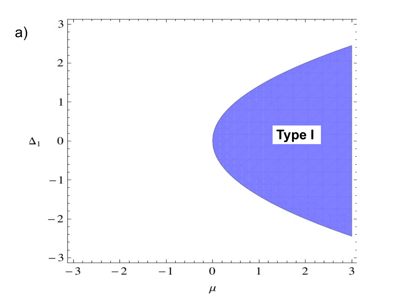
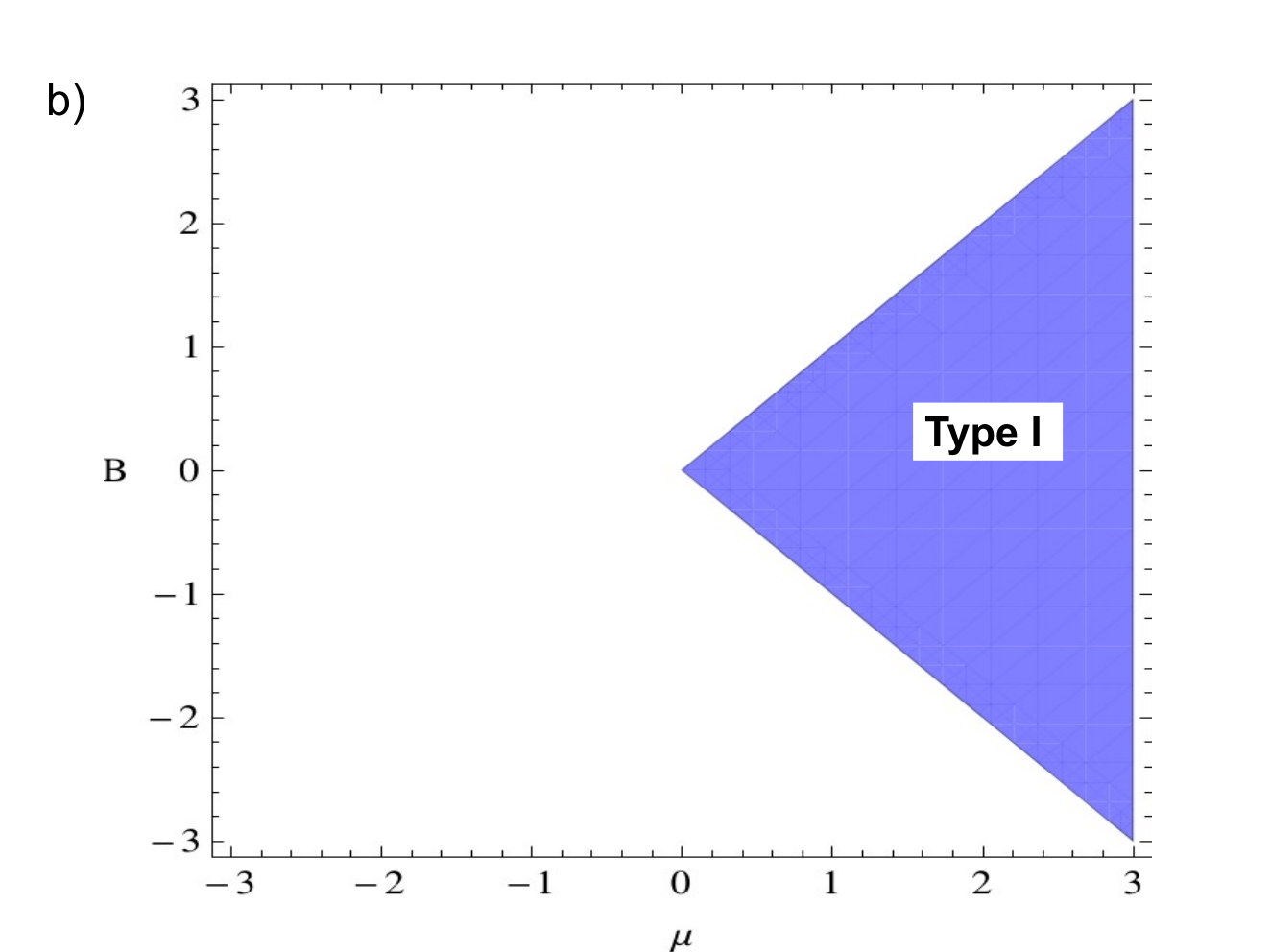
The phase diagram for the MBS in this type of p-wave SC is also the same as in Fig. 2. Below, we list the possible non-trivial topological classes that can arise from certain combinations of s-wave and Zeeman terms. For the trivial classes, refer to Aec. V.

We consider a junction between two spinless p-wave superconductors in 1D. On both sides of the junction we have p-wave superconductor, belonging to BDI class, but there is a phase difference between the order parameters. We consider the junction barrier to be located at $x=0$, having the form $U(x)=U_{0}\delta(x)$ KSG. One can also use the scattering matrix approach in Ref. beenakker; beri, which is essentially the same as the procedure we use here, but with a $\delta$-function potential.

The Hamiltonian on each side of the junction is:

where $\nu\equiv\left[R,L\right]$. Here, we show the calculation for the first kind of p-wave, given as Case I in Sec. II.1. However, one can do an exact same calculation for the second kind (given in Case II, Sec II.2) and get the same form of the subgap states, with the eigenvectors in Eq. III.1 having the structure given in Eq. 11.

Since there is no $\sigma_{x,y}$ term in the Hamiltonian, we consider a single spin species and the trial wave function on each side of the junction is:

where, $k_{\nu}=k_{\nu}^{r}+ik_{\nu}^{I}$ in general. The real part becomes $e^{ik_{\nu}^{r}x}$, giving a plane wave behaviour and the imaginary part becomes $e^{-k_{\nu}^{I}x}$, giving the decaying part. In order to get a decaying solution as $x\rightarrow\infty$, the imaginary part should be positive on the right side of the junction ($x>0$) and negative on the left hand side of the junction ($x<0$). Thus, when we solve the eigenvalue equation for Eq. 15 on each side of the junction, we choose only those values of $k_{\nu}$ for which $k_{R}^{I}>0$ and $k_{L}^{I}<0$. (We will have 4 possible solutions for $k_{\nu}$ on each side, this criterion allows us to pick two among them, on each side.)

Using Eq. 15 and Eq. 16, the eigenvalue equation can be obtained, which gives the possible expressions for $k_{\nu}$ as a function of energy $E$. A general wave function on each side of the junction will be a linear combination of the two possible $k_{\nu}$ modes KSG.

where $k_{R}$ has a positive imaginary part and $k_{L}$ has negative imaginary part. Using Eq. III.1 in the following boundary conditions:

(where, $q_{0}\propto U_{0}$), we get the consistency condition that the determinant from Eq. III.1 should be equal to zero. This gives an equation of the form: $f(E,\mu,\triangle_{0},q_{0},\phi)=0$, from where we get the solutions for $E$ as a function of $\phi$. ($\phi=\phi_{R}-\phi_{L}$)

In Fig. 5, we have calculated $E$ vs. $\phi$ when both Hamiltonians belong to BDI. BDI class has integer number of edge modes, which hybridize across the junction to give a solution as a function of $\phi$. Since $\mu$ in this model is an effective parameter, we do not restrict to the limit when $\mu\rightarrow\infty$. This illuminates more finer features about the subgap states. We look in both limits of the barrier strength, $q_{0}=0$ and $q_{0}$ is high. We see that some features for the strong barrier case when $\mu>\triangle_{0}^{2}/2$ is reciprocated in the weak barrier case when $\mu<\triangle_{0}^{2}/2$ (i.e, $\mu<1/2$, when $\triangle_{0}=1$).

Without loss of generality, we put $\triangle_{0}=1$ and measure all quantities with respect to $\triangle_{0}$. In these units, when $\mu=1$, the solutions for the midgap states are shown in Fig. 5 top panel. If we stick to one branch, it can be seen that energy is $4\pi$ periodic, and is $\sim\cos{\phi/2}$. The bulk bands are at $E=\pm\mu$. When barrier is non-zero, the subgap states are pushed into the bulk bands and the top and bottom parts of the curve get cut off.

When $1/2<\mu<1$, the subgap states are plotted in the middle panel of Fig. 5. They show a similar $4\pi$ periodicity as seen in the previous case, which becomes more apparent when we analytically solve for the solutions putting $q_{0}=0$, in Sec. V.4. Also, we get additional solutions at $E\geq|\sqrt{-1+2\mu}|$. It is interesting to note that for these $E$’s, the form of the subgap states Eq. III.1 changes. That is, one $k$, on each side of the junction, is no longer decaying (has the form $\sim e^{\alpha x}$ for $x>0$), and does not give a physical solution. The other remaining $k$, that gives a decaying solution, is the only physically valid subgap solution. This gives a different set of solutions for the midgap states in the regime $E\geq|\sqrt{-1+2\mu}|$ and $E\leq\mu$. This is what we see in the figure, where for $\mu=0.7$, we see additional states as a function of $\phi$ (additional ‘wings’) close to the bulk bands. We also see the subgap states for $E<|\sqrt{-1+2\mu}|$ end before reaching the bulk bands, i.e, there is a gap between these subgap states and the ‘wing’ like states. The energy scale at which this happens is at $E_{c}=|\sqrt{-1+2\mu}|$, after which there is a sudden change in the functional form of the wave function and also the determinant $f(E,\mu,\triangle_{0},q_{0},\phi)$. For $E>E_{c}$, the minima of the determinant suddenly becomes at $\phi=0$, $2\pi$ and $4\pi$, instead of $\pi$ and $3\pi$. Also, as the barrier strength increases, the nature of these ‘wing’ like states changes. This can be understood from the boundary condition in this region, which effectively gives: $\frac{A_{1}}{A_{2}}=(1-q_{0})\frac{u(k_{L,1})k_{L}}{u(k_{R,1})k_{R}}$. $u(k_{L,1})$ and $u(k_{R,1})$ are also functions of $\phi_{L}$ and $\phi_{R}$, respectively. Depending on $\phi_{R}$ and $\phi_{L}$, a strong barrier can erase the additional states at some $\phi$, and generate them at other $\phi$’s (see, Fig. 5 middle row).

For $\mu<1/2$, the nature of the subgap states change considerably, see Fig. 5 bottom row. Firstly, in the transparent barrier regime, the subgap states merge with the bulk bands ($E=\mu$) earlier, similar to strong barrier regime when $\mu=1$ . Again, we can derive the solutions analytically in the limit $q_{0}=0$ to see that the periodicity is still $4\pi$. Additionally, the nature of the states close to the bulk band do not change drastically. With increasing barrier strength, there is a smooth change of the determinant function and the two minimas merge to one as we move to higher energies. After the energy where it reaches a single minima (as shown by the top and bottom turning points of the lobes), the wavefunctions are no longer valid subgap states. Also with higher barrier strengths, the we get less and less subgap states, shown by the shrinking lobes at high $q_{0}$.

The Hamiltonian on each side of the junction is now of the form Eq. 12. Since in the AIII class there is only one type of zero energy edge states and for all values of $\mu>0$ (shown in Fig. 3), we can linearize around the Fermi points and use the approach described in Ref. beenakker; beri to derive the Andreev reflection matrices across superconducting junctions. We rewrite the Hamiltonian in Eq. 12 in the basis $\begin{pmatrix}c^{\dagger}_{p,\uparrow}&c_{p,\downarrow}&c^{\dagger}_{p,\downarrow}&-c^{\dagger}_{-p,\uparrow}\end{pmatrix}$. The s-wave term takes the form $\triangle_{1}\sigma_{0}\tau_{x}$. The Hamiltonian on each side is of the form:

where, $h_{e}$ and $h_{h}$ are the single-particle Hamiltonians for particle and hole sectors, respectively, and $\triangle$ is the superconducting pair potential. The barrier strength can be tuned to take into account a delta function potential. Between two BDI materials (and also between two AIII materials), when there is two different $\mu$ on the two sides of the junction, there are no subgap states. Also, when there is BDI and AIII on each side of a junction, there are no subgap states.

For cases, when more than one anti-unitary operator is present for a particular symmetry operation, the Hamiltonian needs to be block diagonalized into irreducible diagonal blocks and an effective operator needs to be identified for each such block to get the correct symmetry operation tenfold. For example, let us consider a 1D spinless p-wave BdG Hamiltonian in the presence of a s-wave pairing $\triangle_{1}\sigma_{y}\tau_{y}$,

where, $\sigma$ and $\tau$ are Pauli matrices for the spin and the particle-hole sector, $\triangle_{0}$ and $\mu$ are effective parameters, depending on the underlying heterostructure. The Nambu spinor is $\begin{pmatrix}a^{\dagger}_{k,\uparrow}&a_{-k,\uparrow}&a^{\dagger}_{k,\downarrow}&a_{-k,\downarrow}\end{pmatrix}$, and $\triangle_{0}$ is the magnitude of the p-wave pairing $\triangle_{\uparrow\uparrow}(=\triangle_{\downarrow\downarrow})$. We define the TR operator as an anti-unitary operator which does not mix the particle-hole sector. Whereas, the p-h operator is defined as an anti-unitary operator which rotates the particles into holes and holes into particle sector. It is not necessary for the TR operator to flip spin in all cases, which can be seen from the fact that the unperturbed 1D p-wave Kitaev model is TR invariant. TR operators, satisfying the condition $\mathcal{T}\mathcal{H}(p)\mathcal{T}^{-1}=\mathcal{H}(-p)$, are $\mathcal{T}_{1}=\sigma_{x}\tau_{z}\mathcal{K}$ and $\mathcal{T}_{2}=\sigma_{z}\tau_{z}\mathcal{K}$. The Hamiltonian needs to be block diagonalized in the basis of $U_{\mathcal{T}_{1}}U^{*}_{\mathcal{T}_{2}}$, into $2\times 2$ irreducible blocks, where $U_{\mathcal{T}}$ is the unitary operator for the corresponding TR operator $\mathcal{T}$. The above procedure allows us to diagonalize Eq. 20 into $\sigma_{y}=\pm 1$ blocks: