Optimization of Rate Fairness in Multi-Pair Wireless-Powered Relaying SystemsThanks: This research was supported in part by Basic Science Research Program through the National Research Foundation of Korea (NRF) funded by the Ministry of Education (No. 2017R1D1A1B03030436), in part by the Luxembourg National Research Fund (FNR) in the framework of the FNR-FNRS bilateral project “InWIP-NET: Integrated Wireless Information and Power Networks,” and in part by the Natural Sciences and Engineering Research Council of Canada (NSERC), through its Discovery program. (Corresponding author: Oh-Soon Shin.) V.-P. Bui, H. V. Nguyen, and O.-S. Shin are with the Department of ICMC Convergence Technology and School of Electronic Engineering, Soongsil University, Seoul 06978, South Korea (e-mail: vanphucbui@soongsil.ac.kr; hieuvnguyen@ssu.ac.kr; osshin@ssu.ac.kr). V.-D. Nguyen was with the Department of ICMC Convergence Technology, Soongsil University, Seoul, South Korea. He is now with the Interdisciplinary Centre for Security, Reliability and Trust (SnT) – University of Luxembourg, L-1855 Luxembourg (email: dinh.nguyen@uni.lu). O. A. Dobre is with the Faculty of Engineering and Applied Science, Memorial University, St. John’s, NL A1X3C5, Canada (e-mail: odobre@mun.ca).

Van-Phuc Bui Van-Dinh Nguyen Hieu V. Nguyen Octavia A. Dobre Oh-Soon Shin Affiliation:

Abstract

This letter considers a multi-pair decode-and-forward relay network where a power-splitting (PS) protocol is adopted at the energy-constrained relay to provide simultaneous wireless information and energy harvesting (EH). To achieve higher efficiency of EH, we propose a new PS-based EH architecture at the relay by incorporating an alternating current (AC) computing logic, which is employed to directly use the wirelessly harvested AC energy for computational blocks. Under a nonlinear EH circuit, our goal is to maximize the fairness of end-to-end rate among user pairs subject to power constraints, resulting in a non-convex problem. We propose an iterative algorithm to achieve a suboptimal and efficient solution to this challenging problem by leveraging the inner approximation framework. Numerical results demonstrate that the proposed algorithm outperforms the traditional direct current computing and other baseline schemes.

Index Terms:

Inner approximation, relay network, simultaneous wireless information and power transfer (SWIPT).

I Introduction

Wireless relays have been considered to improve the spectral efficiency and reliability, and to extend the coverage area of wireless networks. Among numerous proposed relaying protocols, decode-and-forward (DF) and amplify-and-forward are most widely studied in the literature. The former has drawn considerable attention due to its superior performance compared to the latter [1].

With the dramatic growth of user devices, especially those with low-cost and low-power requirements, we can envisage future networks employing wireless relays capable of using harvested power for information forwarding, rather than depending on the grid power supply. To this end, simultaneous wireless information and power transfer (SWIPT) technique is an effective means to realize both energy harvesting (EH) and information decoding from the transmitted radio-frequency (RF) signals, prolonging the network lifetime of relays [2, 3, 4]. Various SWIPT-based relay schemes based on time-switching relaying (TSR) and power-splitting relaying (PSR) have been proposed, including multiple-input multiple-output (MIMO) DF relay [5], self interference-aided EH relaying [6], and relays with interference alignment [7]. The common approach in the aforementioned works is that the EH power circuit converts the harvested alternating current (AC) power to direct current (DC) power to assist user data transmission and activate basic functions (i.e., operating circuits and computational blocks). Given that the wireless EH performance is very limited due to high path-loss in far-field transmission, the use of DC computing (DCC) results in significant system performance loss. The reason is that the conversion efficiency of current rectifiers is relatively low (i.e., about $50\sim 60\%$ ). Fortunately, the works in [8] and [9] have demonstrated through practical experiments that the AC power harvested from the RF signals can be directly used to activate computational blocks. The benefit of using AC computing (ACC) was first revealed in downlink SWIPT [10] and NOMA-SWIPT networks [11].

Motivated by the above discussion, we study a multi-pair wireless-powered relaying system, where a multiple-antenna DF relay receives both information and energy from source nodes in the first phase and then utilizes the energy to forward the information to destination nodes in the second phase. Contrary to the previous works on SWIPT-based relay networks [2, 5, 6, 7], this letter poses the following completely new issues: $(i)$ A novel PSR architecture-enabled ACC is proposed by leveraging charge-recycling theory, which aims at using the EH more efficiently due to its low-power consumption and no conversion loss; $(ii)$ Successive interference cancellation (SIC) technique is adopted at the information decoding (ID) receiver [12], which is capable of improving both spectral efficiency and user fairness. We consider a new problem of max-min end-to-end (e2e) rate among user pairs under a practical model of EH circuit [13], which is formulated as a non-convex program. Towards an efficient solution, we convert the original problem into an equivalent non-convex problem in a more tractable form, and then develop a lowcomplexity iterative algorithm with convergence guaranteed. By leveraging the inner approximation (IA) framework [14], the proposed algorithm solves a second order cone program (SOCP) at each iteration, which is very efficient for practical implementations. Numerical results are provided to confirm that our proposed algorithm is efficient in terms of the e2e rate fairness.

II System Model and Problem Formulation

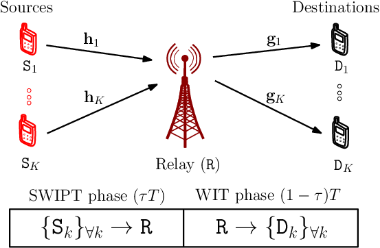
We consider a multi-pair wireless-powered relaying network, which consists of one energy-constrained DF relay $\mathtt{R}$ equipped with $N$ antennas and the set $\mathcal{K}\triangleq\{1,\dots,K\}$ of $K=|\mathcal{K}|$ single-antenna user pairs, as illustrated in Fig. 1. In the $k$ -th user pair, we assume that the source node $\mathtt{S}_{k}$ communicates with the destination node $\mathtt{D}_{k}$ via $\mathtt{R}$ and there is no direct link between $\mathtt{S}_{k}$ and $\mathtt{D}_{k}$ due to path-loss and shadowing. The channels from $\mathtt{S}_{k}\rightarrow\mathtt{R}$ and $\mathtt{R}\rightarrow\mathtt{D}_{k}$ are denoted by $\mathbf{h}_{k}\in\mathbb{C}^{N\times 1}$ and $\mathbf{g}_{k}\in\mathbb{C}^{1\times N}$ , respectively, which are assumed to change block-by-block. The transmission block time, denoted by $T$ , is divided into two phases: SWIPT phase $(\tau T)$ from $\{\mathtt{S}_{k}\}_{k\in\mathcal{K}}\rightarrow\mathtt{R}$ and wireless information transfer (WIT) phase $(1-\tau)T$ from $\mathtt{R}\rightarrow\{\mathtt{D}_{k}\}_{k\in\mathcal{K}}$ , where $\tau\in(0,1)$ is a fraction of block time.

II-A System Model

Refer to caption — Fig. 1: A multi-pair DF relaying network with SWIPT and WIT phases.

II-A1 SWIPT Phase

In Fig. 2, we propose a new PSR architecture which enables the SIC technique and ACC logic at the ID and EH receivers, respectively. In particular, the received RF signal at $\mathtt{R}$ is split into two parts: ID and EH signals. In the EH receiver, the energy harvesting and distribution blocks split the harvested AC power into two flows: one to directly supply the wirelessly harvested AC power for the ACC logic without rectification and regulation, while other to charge the battery for transmitting signals in the WIT phase by using the AC-to-DC rectifier. Note that the use of ACC logic eliminates the EH conversion loss. Let $\alpha\in(0,1)$ be a portion of the RF signal $\mathbf{y}_{\mathtt{R}}$ received at the relay using a power splitter. The ID and EH signals can be expressed as:

\displaystyle\mathbf{y}_{\mathtt{R}}^{\mathtt{ID}}=\sqrt{\alpha}\mathbf{y}_{\mathtt{R}}+\mathbf{n}_{\mathtt{R}}\quad\text{and}\quad\mathbf{y}_{\mathtt{R}}^{\mathtt{EH}}=\sqrt{1-\alpha}\mathbf{y}_{\mathtt{R}},

(1)

where $\mathbf{y}_{\mathtt{R}}=\sum_{k\in\mathcal{K}}p_{k}\mathbf{h}_{k}s_{k}+\mathbf{n}_{\mathtt{Ant}}$ . Here $p_{k}$ and $s_{k}$ with $\mathbb{E}\{|s_{k}|^{2}\}=1$ are the transmit power coefficient and the transmitted symbol at $\mathtt{S}_{k}$ , respectively; $\mathbf{n}_{\mathtt{Ant}}\sim\mathcal{CN}(0,\sigma^{2}_{\mathtt{Ant}}\mathbf{I})$ and $\mathbf{n}_{\mathtt{R}}\sim\mathcal{CN}(0,\sigma^{2}_{\mathtt{R}}\mathbf{I})$ are the antenna noise and additional circuit noise introduced by the ID receiver, which are modeled as additive white Gaussian noise (AWGN) [15]. Without loss of generality, we normalize $T$ to 1 and rearrange the users in the ascending order of their channel gains, i.e., $\|\mathbf{h}_{1}\|^{2}_{2}\leq\cdots\leq\|\mathbf{h}_{k}\|_{2}^{2}\cdots\leq\|\mathbf{h}_{K}\|^{2}_{2}$ . We adopt the minimum mean square error and SIC (MMSE-SIC) technique at the ID receiver to decode signals from sources [12]. To enhance the user fairness, we assume that the decoding order of SIC is from $s_{K}$ to $s_{1}$ . Hence, the data rate (measured in nats/sec/Hz) in decoding $s_{k}$ at $\mathtt{R}$ is given as

\displaystyle R_{1,k}(\mathbf{p},\tau,\alpha)=\tau\ln\bigl(1+\gamma_{1,k}(\mathbf{p},\alpha)\bigl),

(2)

where ${\gamma}_{1,k}(\mathbf{p},\alpha)=p_{k}^{2}\mathbf{h}_{k}^{H}\boldsymbol{\Phi}_{k}^{-1}\mathbf{h}_{k}$ with $\boldsymbol{\Phi}_{k}\triangleq\sum\nolimits_{\ell=1}^{k-1}p_{\ell}^{2}\mathbf{h}_{\ell}\mathbf{h}_{\ell}^{H}+\sigma_{\mathtt{Ant}}^{2}\mathbf{I}+\frac{\sigma^{2}_{\mathtt{R}}}{\alpha}\mathbf{I}$ and $\mathbf{p}\triangleq\{p_{k}\}_{k\in\mathcal{K}}$ .

Next, the EH signal is further split into two flows by the energy harvester and distribution block, which are $\sqrt{\beta}\mathbf{y}_{\mathtt{R}}^{\mathtt{EH}}$ with the fraction $\beta\in(0,1)$ to directly supply an AC voltage to the ACC and the remaining $\sqrt{1-\beta}\mathbf{y}_{\mathtt{R}}^{\mathtt{EH}}$ to be rectified to the DC power. The DC power is stored in a rechargeable battery to be used for the data transmission in the WIT phase. By the charge-recycling theory [8, 9], the average harvested AC power supplying ACC can be expressed as

\displaystyle P_{\mathtt{R}}^{\mathtt{ACC}}(\mathbf{p},\tau,1-\alpha,\beta)=\tau(1-\alpha)\beta\sum_{k\in\mathcal{K}}p_{k}^{2}\|\mathbf{h}_{k}\|^{2}_{2}.

(3)

Considering a realistic nonlinear EH model [13], the average harvested DC power at the EH receiver can be calculated as

	$\displaystyle P_{\mathtt{R}}^{\mathtt{DC}}(\mathbf{p},\tau,1-\alpha,1-\beta)=\tau\mathord{\raise 0.49991pt\hbox{$\displaystyle\genfrac{}{}{0.4pt}{}{\bar{P}_\mathtt{EH}^{\max}}{1-\Omega}$}}$
	$\displaystyle\hskip 18.49988pt\hskip 18.49988pt\hskip 9.24994pt\times\Big(\mathord{\raise 0.49991pt\hbox{$\displaystyle\genfrac{}{}{0.4pt}{}{1}{1+\exp\bigl(-a(P_\mathtt{R}^{\mathtt{IN}}(\bp,1-\alpha,1-\beta)-b)\bigr)}$}}-\Omega\Big),$		(4)

where $P_{\mathtt{R}}^{\mathtt{IN}}(\mathbf{p},1-\alpha,1-\beta)\triangleq(1-\alpha)(1-\beta)\sum\nolimits_{k\in\mathcal{K}}p_{k}^{2}\|\mathbf{h}_{k}\|_{2}^{2}$ is the AC power at the input of the EH circuit, $\bar{P}_{\mathtt{EH}}^{\max}$ is the maximum harvested power, the constants $a$ and $b$ specify the EH circuits, and $\Omega=\bigr(1+\exp(ab)\bigl)^{-1}$ .

II-A2 WIT Phase

The relay re-encodes signals and forwards them to the destinations using the harvested power in the SWIPT phase. The re-encoded signal of the $k$ -th pair is linearly weighted with the beamformer $\mathbf{w}_{k}\in\mathbb{C}^{N\times 1}$ at the relay prior to being forwarded to $\mathtt{D}_{k}$ . As a result, the data rate decoded by $\mathtt{D}_{k}$ is given as

\displaystyle R_{2,k}(\mathbf{w},1-\tau)=(1-\tau)\ln\bigl(1+\gamma_{2,k}(\mathbf{w})\bigr),

(5)

where $\gamma_{2,k}(\mathbf{w})\triangleq\frac{|\mathbf{g}_{k}\mathbf{w}_{k}|^{2}}{\sum\nolimits_{\ell\in\mathcal{K}\backslash k}|\mathbf{g}_{k}\mathbf{w}_{\ell}|^{2}+\sigma_{k}^{2}}$ , $\mathbf{w}\triangleq\{\mathbf{w}_{k}\}_{k\in\mathcal{K}}$ and $\sigma_{k}^{2}$ is the variance of the AWGN at $\mathtt{D}_{k}$ .

Remark 1

The use of power domain-based NOMA at destinations [11] is inefficient since the harvested energy at the relay is very limited. It is noted that in multi-user SWIPT-based relay networks, the better the EH performance is, the more severer the network interference at the relay is.

II-B Optimization Problem Formulation

The achievable e2e rate of the $k$ -th pair can be defined as

\displaystyle R_{k}=\min\big\{R_{1,k}(\mathbf{p},\tau,\alpha),R_{2,k}(\mathbf{w},1-\tau)\big\},\quad\forall k\in\mathcal{K}.

(6)

The average power consumed by the relay can be expressed as

\displaystyle{P_{\mathtt{R}}^{\mathtt{tot}}(\mathbf{w},1-\tau)=(1-\tau)P_{\mathtt{R}}^{\mathtt{BF}}(\mathbf{w})+P_{\mathtt{R}}^{\mathtt{sta}},}

(7)

where $P_{\mathtt{R}}^{\mathtt{BF}}(\mathbf{w})\triangleq\sum\nolimits_{k\in\mathcal{K}}\|\mathbf{w}_{k}\|^{2}_{2}$ and $P_{\mathtt{R}}^{\mathtt{sta}}$ are the radiated power in the WIT phase and the static power consumed by the circuits at $\mathtt{R}$ , respectively.

We can observe that all parameters are mutually dependent, and thus, should be jointly optimized. The optimization problem of maximizing the minimum e2e rate among all user pairs can be mathematically expressed as


$\displaystyle\max\limits_{\mathbf{p},\mathbf{w},\tau,\alpha,\beta}$	r_0≜min_k∈K {R_k}	(8a)
$\displaystyle{\mathrm{s.t.}}$	P_R^tot(w,1-τ) ≤P_R^DC(p,τ,1-α,1-β),	(8b)
P_R^ACC(p,τ, 1-α,β) ≥P^ACC_min,		(8c)
p_k^2 ≤P_S_k^max, ∀k∈K		(8d)
τ∈(0,1), α∈(0,1), β∈(0,1).		(8e)

Here constraint (8b) ensures that the power consumption cannot exceed the harvested power. $P^{\mathtt{ACC}}_{\min}$ in (8c) is the minimum AC power required for the ACC, while (8d) represents the transmit power constraint at the source nodes.

Remark 2

The optimization problem with the traditional DCC can also be formulated as

	$\displaystyle\max\limits_{\mathbf{p},\mathbf{w},\tau,\alpha,\beta=0}\hskip 9.24994pt\tilde{r}_{0}\triangleq\min\limits_{k\in\mathcal{K}}\ \{R_{k}\},\hskip 9.24994pt{\mathrm{s.t.}}\ \eqref{MMRd},\eqref{MMRe},$
	$\displaystyle\hskip 18.49988pt\&\ P_{\mathtt{R}}^{\mathtt{tot}}(\mathbf{w},1-\tau)+P^{\mathtt{DCC}}_{\min}\leq P_{\mathtt{R}}^{\mathtt{DC}}(\mathbf{p},\tau,1-\alpha,1),\hskip 18.49988pt$		(9)

where $\beta=0$ and $P^{\mathtt{DCC}}_{\min}$ is the minimum DC power required for DCC. In addition to no EH conversion loss by the use of ACC, the benefit of problem (8) over (2) can be realized by the fact that $P^{\mathtt{DCC}}_{\min}$ is much higher than $P^{\mathtt{ACC}}_{\min}$ [9].

III Proposed Algorithm

III-A Equivalent Formulation

Problem (8) is a non-convex program due to the non-concave and non-smooth objective (8a) and non-convex constraints (8b) and (8c). A direct application of the proposed method in [11] for solving (8) still involves a nonconvex problem due to strong coupling between optimization variables, and thus, several preliminary steps are necessary. For that, we first make change of variables as $\tau_{1}=\tau^{-1},\tau_{2}=(1-\tau)^{-1},\alpha_{1}=\alpha^{-1},\alpha_{2}=(1-\alpha)^{-1}$ , and introduce the slack variables $\psi_{1,k}>0,{\psi}_{2,k}>0,\forall k$ and $r\geq 0$ to rewrite (8) into the following equivalent problem:

	$\displaystyle\max_{\mathbf{p},\mathbf{w},\boldsymbol{\tau},\boldsymbol{\alpha},\boldsymbol{\psi},\beta,r}\quad r$		(10a)
	$\displaystyle\quad{\mathrm{s.t.}}\ \tau_{i}^{-1}\ln\bigl(1+\psi_{i,k}^{-1}\bigr)\geq r,\ \forall i\in\mathcal{I}\triangleq\{1,2\},k\in\mathcal{K},\qquad$		(11a)
	$\displaystyle\qquad\quad\gamma_{1,k}(\mathbf{p},\alpha_{1}^{-1})\geq\psi_{1,k}^{-1},\ \forall k\in\mathcal{K},$		(12a)
	$\displaystyle\qquad\quad\gamma_{2,k}(\mathbf{w})\geq\psi_{2,k}^{-1},\ \forall k\in\mathcal{K},$		(13a)
	$\displaystyle\qquad\quad P_{\mathtt{R}}^{\mathtt{tot}}(\mathbf{w},\tau_{2}^{-1})\leq P_{\mathtt{R}}^{\mathtt{DC}}(\mathbf{p},\tau_{1}^{-1},\alpha_{2}^{-1},1-\beta),\qquad$		(14a)
	$\displaystyle\qquad\quad P_{\mathtt{R}}^{\mathtt{ACC}}(\mathbf{p},\tau_{1}^{-1},\alpha_{2}^{-1},\beta)\geq P^{\mathtt{ACC}}_{\min},$		(15a)
	$\displaystyle\qquad\quad\tau_{1}^{-1}+\tau_{2}^{-1}\leq 1,\tau_{1}>1,\tau_{2}>1,$		(16a)
	$\displaystyle\qquad\quad\alpha_{1}^{-1}+\alpha_{2}^{-1}\leq 1,\alpha_{1}>1,\alpha_{2}>1,$		(17a)
	$\displaystyle\qquad\quad\beta\in(0,1),\ p_{k}^{2}\leq P_{\mathtt{S}_{k}}^{\max},\quad\forall k\in\mathcal{K},$		(18a)

where $\boldsymbol{\tau}\triangleq\{\tau_{i}\}_{i\in\mathcal{I}}$ , $\boldsymbol{\alpha}\triangleq\{\alpha_{i}\}_{i\in\mathcal{I}}$ and $\boldsymbol{\psi}\triangleq\{\psi_{i,k}\}_{i\in\mathcal{I},k\in\mathcal{K}}$ . We now provide the following lemma to characterize the key property of problem (10a).

Lemma 1

The optimization problems (8) and (10a) are equivalent, as they share the same optimal solution set and objective value (i.e., $r_{0}^{\star}=r^{\star}$ ).

Proof:

See Appendix.∎

III-B IA-based Iterative Algorithm

In problem (10a), the non-convex constraints include (11a)-(15a). Let us handle the non-convex constraint (11a) first. We can see that the function $f(\psi_{i,k},\tau_{i})\triangleq\tau_{i}^{-1}\ln\bigl(1+\psi_{i,k}^{-1}\bigr)$ is convex on the domain $(\tau_{i}>1,\psi_{i,k}>0)$ , which is useful to develop an approximate solution by the IA method. At iteration $\kappa$ of an iterative algorithm presented shortly, (11a) is innerly approximated as

\displaystyle f^{(\kappa)}(\psi_{i,k},\tau_{i})\triangleq A^{(\kappa)}+B^{(\kappa)}\psi_{i,k}+C^{(\kappa)}\tau_{i}\geq r,\ \forall i,k,\quad

(19)

where $A^{(\kappa)}\triangleq 2\ln\big(1+1/\psi_{i,k}^{(\kappa)}\big)/\tau_{i}^{(\kappa)}+1/(\psi_{i,k}^{(\kappa)}+1)\tau_{i}^{(\kappa)}$ , $B^{(\kappa)}\triangleq-1/\psi_{i,k}^{(\kappa)}(\psi_{i,k}^{(\kappa)}+1)\tau_{i}^{(\kappa)}$ and $C^{(\kappa)}\triangleq-\ln\big(1+1/\psi_{i,k}^{(\kappa)}\big)/(\tau_{i}^{(\kappa)})^{2}$ are constant. Note that $f^{(\kappa)}(\psi_{i,k},\tau_{i})$ in (19) is concave and represents a global lower bound of $f(\psi_{i,k},\tau_{i})$ at the feasible point $(\psi_{i,k}^{(\kappa)},\tau_{i}^{(\kappa)})$ [16, Appendix A], satisfying $f^{(\kappa)}(\psi_{i,k}^{(\kappa)},\tau_{i}^{(\kappa)})=f(\psi_{i,k}^{(\kappa)},\tau_{i}^{(\kappa)})$ .

Next, we tackle the non-convexity of (12a) and (13a). For (12a), we first consider the function $h(p_{k},\bar{\boldsymbol{\Phi}}_{k})\triangleq p_{k}^{2}\mathbf{h}_{k}^{H}\bar{\boldsymbol{\Phi}}_{k}^{-1}\mathbf{h}_{k}$ with $p_{k}>0$ and $\boldsymbol{\bar{\Phi}}_{k}\triangleq\sum\nolimits_{\ell=1}^{k-1}p_{\ell}^{2}\mathbf{h}_{\ell}\mathbf{h}_{\ell}^{H}+\sigma_{\mathtt{Ant}}^{2}\mathbf{I}+\alpha_{1}\sigma^{2}_{\mathtt{R}}\mathbf{I}\succ\mathbf{0}$ . A concave approximate function of $h(p_{k},\bar{\boldsymbol{\Phi}}_{k})$ is given as

	$\displaystyle h(p_{k},\bar{\boldsymbol{\Phi}}_{k})\geq h^{(\kappa)}(p_{k},\bar{\boldsymbol{\Phi}}_{k})\triangleq 2p_{k}^{(\kappa)}\mathbf{h}_{k}^{H}(\bar{\boldsymbol{\Phi}}_{k}^{(\kappa)})^{-1}\mathbf{h}_{k}p_{k}$
	$\displaystyle-(p_{k}^{(\kappa)})^{2}\mathbf{h}_{k}^{H}(\bar{\boldsymbol{\Phi}}_{k}^{(\kappa)})^{-1}\bar{\boldsymbol{\Phi}}_{k}(\bar{\boldsymbol{\Phi}}_{k}^{(\kappa)})^{-1}\mathbf{h}_{k},\quad$		(20)

where $\boldsymbol{\bar{\Phi}}_{k}^{(\kappa)}\triangleq\sum\nolimits_{\ell=1}^{k-1}(p_{\ell}^{(\kappa)})^{2}\mathbf{h}_{\ell}\mathbf{h}_{\ell}^{H}+\sigma_{\mathtt{Ant}}^{2}\mathbf{I}+\alpha_{1}^{(\kappa)}\sigma^{2}_{\mathtt{R}}\mathbf{I}$ . The proof is done by the fact that $h(p_{k},\bar{\boldsymbol{\Phi}}_{k})$ is a convex function in $(p_{k},\bar{\boldsymbol{\Phi}}_{k})$ [17, Eq. (31)]. Therefore, we can iteratively replace (12a) with the following convex constraint:

\displaystyle h^{(\kappa)}(p_{k},\bar{\boldsymbol{\Phi}}_{k})\geq 1/\psi_{1,k},\ \forall k\in\mathcal{K}.

(21)

We rewrite (13a) as $(\Re\{\mathbf{g}_{k}\mathbf{w}_{k}\})^{2}\geq\frac{\sum_{\ell\in\mathcal{K}\backslash k}|\mathbf{g}_{k}\mathbf{w}_{\ell}|^{2}+\sigma_{k}^{2}}{\psi_{2,k}}$ , which can be convexified as

\displaystyle g^{(\kappa)}(\mathbf{w}_{k})\geq\frac{\sum_{\ell\in\mathcal{K}\backslash k}|\mathbf{g}_{k}\mathbf{w}_{\ell}|^{2}+\sigma_{k}^{2}}{\psi_{2,k}},\ \forall k\in\mathcal{K},

(22)

upon the condition

\displaystyle\Re\{\mathbf{g}_{k}^{H}\mathbf{w}_{k}\}\geq 0,\ \forall k\in\mathcal{K},

(23)

where $g^{(\kappa)}(\mathbf{w}_{k})\triangleq 2\Re\{\mathbf{g}_{k}\mathbf{w}^{(\kappa)}_{k}\}\Re\{\mathbf{g}_{k}\mathbf{w}_{k}\}-(\Re\{\mathbf{g}_{k}\mathbf{w}^{(\kappa)}_{k}\})^{2}$ is the concave approximation of $(\Re\{\mathbf{g}_{k}\mathbf{w}_{k}\})^{2}$ at $\mathbf{w}^{(\kappa)}_{k}$ .

We are now in a position to approximate (14a) and (15a). It is true that

$\displaystyle\eqref{MMReqi:e}\Leftrightarrow$	$\displaystyle a\sum_{k\in\mathcal{K}}\frac{p_{k}^{2}\\|\mathbf{h}_{k}\\|_{2}^{2}}{\alpha_{2}}+\ln\bigl(\frac{1}{\vartheta}\bigr)\frac{1}{1-\beta}\geq\frac{ab}{1-\beta},$	(24aa)
$\displaystyle\eqref{MMReqi:e}\Leftrightarrow$	$\displaystyle(\tau_{2}-1)\vartheta\geq(1+\vartheta)\theta,$	(24ba)
$\displaystyle\eqref{MMReqi:e}\Leftrightarrow$	$\displaystyle\xi\theta-\xi\Omega(\tau_{2}-1)-\tau_{2}P_{\mathtt{R}}^{\mathtt{sta}}\geq P_{\mathtt{R}}^{\mathtt{BF}}(\mathbf{w}),$	(24ca)

where $\xi\triangleq\frac{\bar{P}_{\mathtt{EH}}^{\max}}{1-\Omega}$ , and $\vartheta$ and $\theta$ are slack variables. Constraint (24ca) is convex, while (24aa) and (24ba) still remain non-convex. By applying the first-order Taylor series approximation to the non-convex parts of (24aa) and an approximation of bilinear function $(1+\vartheta)\theta$ of (24ba) [14], it follows that

	$\displaystyle a\mathcal{H}^{(\kappa)}(\mathbf{p},\alpha_{2})+\tilde{f}^{(\kappa)}(\vartheta,\beta)$	$\displaystyle\geq$	$\displaystyle\frac{ab}{1-\beta},\qquad$		(25a)
	$\displaystyle(\tau_{2}-1)\vartheta$	$\displaystyle\geq$	$\displaystyle\mathcal{B}^{(\kappa)}(1+\vartheta,\theta),$		(26a)

where $\mathcal{H}^{(\kappa)}(\mathbf{p},\alpha_{2})\triangleq\sum_{k\in\mathcal{K}}\Big(\frac{2p_{k}^{(\kappa)}\|\mathbf{h}_{k}\|_{2}^{2}}{\alpha_{2}^{(\kappa)}}p_{k}-\frac{(p_{k}^{(\kappa)})^{2}\|\mathbf{h}_{k}\|_{2}^{2}}{(\alpha_{2}^{(\kappa)})^{2}}\alpha_{2}\Big)$ , $\tilde{f}^{(\kappa)}(\vartheta,\beta)\triangleq 2\ln\big(\mathord{\raise 0.49991pt\hbox{$\displaystyle\genfrac{}{}{0.4pt}{}{1}{\varthetai}$}}\big)\mathord{\raise 0.49991pt\hbox{$\displaystyle\genfrac{}{}{0.4pt}{}{1}{1-\betai}$}}-\mathord{\raise 0.49991pt\hbox{$\displaystyle\genfrac{}{}{0.4pt}{}{\vartheta}{\varthetai(1-\betai)}$}}+\mathord{\raise 0.49991pt\hbox{$\displaystyle\genfrac{}{}{0.4pt}{}{1}{1-\betai}$}}-\ln\big(\mathord{\raise 0.49991pt\hbox{$\displaystyle\genfrac{}{}{0.4pt}{}{1}{\varthetai}$}}\big)\mathord{\raise 0.49991pt\hbox{$\displaystyle\genfrac{}{}{0.4pt}{}{1-\beta}{(1-\betai)^2}$}}$ and $\mathcal{B}^{(\kappa)}(1+\vartheta,\theta)\triangleq 0.5\bigl(\frac{1+\vartheta^{(\kappa)}}{\theta^{(\kappa)}}\theta^{2}+\frac{\theta^{(\kappa)}}{1+\vartheta^{(\kappa)}}(1+\vartheta)^{2}\bigr)$ . Finally, we can transform (15a) into $\sum_{k\in\mathcal{K}}\frac{p_{k}^{2}\|\mathbf{h}_{k}\|_{2}^{2}}{\alpha_{2}}\geq P^{\mathtt{ACC}}_{\min}\frac{\tau_{1}}{\beta}$ , which is innerly approximated as

\displaystyle\mathcal{H}^{(\kappa)}(\mathbf{p},\alpha_{2})\geq P^{\mathtt{ACC}}_{\min}\mathcal{B}^{(\kappa)}(\tau_{1},1/\beta),

(27)

by following the same procedures as in (25a).

Summing up, at iteration $\kappa+1$ , we solve the following approximate convex program:

	$\displaystyle\max_{\mathbf{s},r}\quad r$		(28a)
	$\displaystyle{\mathrm{s.t.}}\ \eqref{MMReqi:g}-\eqref{MMReqi:i},\eqref{MMReqi:bconvex},\eqref{eq:approhfunction},\eqref{std1},\eqref{std2},\eqref{MMReqi:e1c},\eqref{MMReqi:e2},\eqref{MMReqi:fconvex},\qquad$		(29a)

where $\mathbf{s}\triangleq\{\mathbf{p},\mathbf{w},\boldsymbol{\tau},\boldsymbol{\alpha},\boldsymbol{\psi},\beta,\vartheta,\theta\}$ denotes the set of variables that needs to be updated in the next iteration. We can see that the main barrier in finding an initial feasible point to start the computational procedure for (10a) is due to constraint (15a). Therefore, we successively solve the following modified convex program of (28a):

	$\displaystyle\max_{\mathbf{s},r}\quad\eta\triangleq\mathcal{H}^{(\kappa)}(\mathbf{p},\alpha_{2})-P^{\mathtt{ACC}}_{\min}\mathcal{B}^{(\kappa)}(\tau_{1},1/\beta)$		(30a)
	$\displaystyle{\mathrm{s.t.}}\ \eqref{MMReqi:g}-\eqref{MMReqi:i},\eqref{MMReqi:bconvex},\eqref{eq:approhfunction},\eqref{std1},\eqref{std2},\eqref{MMReqi:e1c},\eqref{MMReqi:e2},\qquad$		(31a)

until reaching $\eta\geq 0$ . To efficiently solve (30a), we first set $p_{k}^{(0)}=\sqrt{P_{\mathtt{S}_{k}}^{\max}},\forall k,\tau_{1}^{(0)}=\tau_{2}^{(0)}=\alpha_{1}^{(0)}=\alpha_{2}^{(0)}=2,\beta=0.5$ , and randomly generate a sufficiently small value of $\mathbf{w}^{(0)}$ to ensure that (14a) is feasible. Other initial points can be found as $\psi_{1,k}^{(0)}=1/\gamma_{1,k}(\mathbf{p}^{(0)},1/\alpha_{1}^{(0)}),\psi_{2,k}^{(0)}=1/\gamma_{2,k}(\mathbf{w}^{(0)})$ , $\vartheta^{(0)}=1/\exp\bigl(-a(P_{\mathtt{R}}^{\mathtt{IN}}(\mathbf{p}^{(0)},1/\alpha_{2}^{(0)},1-\beta^{(0)})-b)\bigr)$ , and $\theta^{(0)}=(\tau_{2}^{(0)}-1)\vartheta^{(0)}/(1+\vartheta^{(0)})$ by setting inequalities (12a), (13a), (24aa) and (24ba) to equalities, respectively. The proposed iterative algorithm is summarized in Algorithm 1.

0: Set

\kappa:=0,\kappa^{\prime}:=0

and randomly generate

\mathbf{s}^{(0)}

1: repeat

2: Solve (30a) to obtain the optimal solution

\mathbf{s}^{\star}

3: Update

\mathbf{s}^{(\kappa^{\prime}+1)}:=\mathbf{s}^{\star}

and set

\kappa^{\prime}:=\kappa^{\prime}+1.

4: until

\eta\geq 0

5: Set

\mathbf{s}^{(0)}:=\mathbf{s}^{(\kappa^{\prime})}

6: repeat

7: Solve (28a) to obtain the optimal solution

\mathbf{s}^{\star}.

8: Update

\mathbf{s}^{(\kappa+1)}:=\mathbf{s}^{\star}

and set

\kappa:=\kappa+1.

9: until Convergence

10: Output:

(\mathbf{p},\mathbf{w},\tau,\alpha,\beta):=\bigl(\mathbf{p}^{(\kappa)},\mathbf{w}^{(\kappa)},\frac{1}{\tau_{1}^{(\kappa)}},\frac{1}{\alpha_{1}^{(\kappa)}},\beta^{(\kappa)}\bigl)

Algorithm 1 Proposed Iterative Algorithm for Solving (8)

Remark 3

We note that problem (28a) can be transformed into an SOCP, where modern convex solvers are very efficient. The key is to further transform constraints (16a), (17a), (21) and (27) into SOC ones:

		$\displaystyle\eqref{MMReqi:g}\Leftrightarrow\tilde{\tau}_{1}+\tilde{\tau}_{2}\leq 1,\ \&\ \tilde{\tau}_{1}\tau_{1}\geq 1,\ \&\ \tilde{\tau}_{2}\tau_{2}\geq 1,$
		$\displaystyle\eqref{MMReqi:h}\Leftrightarrow\tilde{\alpha}_{1}+\tilde{\alpha}_{2}\leq 1,\ \&\ \tilde{\alpha}_{1}\alpha_{1}\geq 1,\ \&\ \tilde{\alpha}_{2}\alpha_{2}\geq 1,$
		$\displaystyle\eqref{eq:approhfunction}\Leftrightarrow h^{(\kappa)}(p_{k},\bar{\boldsymbol{\Phi}}_{k})\geq\tilde{\psi}_{1,k},\ \&\ \psi_{1,k}\tilde{\psi}_{1,k}\geq 1,\forall k\in\mathcal{K},$
		$\displaystyle\eqref{MMReqi:fconvex}\Leftrightarrow\mathcal{H}^{(\kappa)}(\mathbf{p},\alpha_{2})\geq P^{\mathtt{ACC}}_{\min}\mathcal{B}^{(\kappa)}(\tau_{1},\tilde{\beta}),\ \&\ \beta\tilde{\beta}\geq 1,$

where $\tilde{\tau}_{i},\tilde{\alpha}_{i},\forall i\in\mathcal{I},\tilde{\psi}_{1,k},\forall k\in\mathcal{K}$ and $\tilde{\beta}$ are slack variables.

Convergence and Complexity Analysis: We can see that all the convex approximations in (28a) satisfy the IA properties listed in [14]. In other words, the optimal solution obtained at iteration $\kappa$ of Algorithm 1 is also feasible for problem (28a) at iteration $\kappa+1$ . It implies that Algorithm 1 produces a sequence $\mathbf{s}^{(\kappa)}$ of improved points of (8), which converges to at least a local optimum. Problem (28a) involves $(6K+7)$ conic constraints and $(KN+3K+8)$ scalar decision variables. Thus, the worst-case computational complexity in each iteration of Algorithm 1 is $\mathcal{O}\bigl((6K)^{0.5}(KN+3K)^{3}\bigr)$ . Similarly, the complexity of (30a) for finding an initial feasible point is $\mathcal{O}\bigl((6K)^{0.5}(KN+3K)^{3}\bigr)$ .

Remark 4

The channel state information (CSI) between the relay and sources/destinations, as well as the controlling signal, can be exchanged via dedicated channels, and thus the algorithm is simply executed at the relay. Moreover, Algorithm 1 can be slightly modified to solve the worst-case robust optimization problem, where the bounded CSI error is taken into account.

IV Numerical Results

We consider the relay network as shown in Fig. 1, in which the distances from each source to relay and from the relay to each destination are set to be 10 m and 15 m, respectively. The networks parameters are set as $K=4$ , $\sigma_{\mathtt{Ant}}^{2}=\sigma_{k}^{2}=-70$ dBm, $\sigma^{2}_{\mathtt{R}}=-50$ dBm, $P_{\mathtt{R}}^{\mathtt{sta}}=1$ $\mu$ W, $P^{\mathtt{ACC}}_{\min}=0.27$ $\mu$ W and $P^{\mathtt{DCC}}_{\min}=47.64$ $\mu$ W [9, 15]. The parameters of nonlinear EH model are $\bar{P}^{\max}_{\mathtt{EH}}=0.2$ mW, $a$ = 6400 and $b=0.003$ [13]. All channels are assumed to undergo Rayleigh fading with the path-loss exponent of 3.5. All source nodes are assumed to have the same power budget, i.e., $P_{\mathtt{S}}^{\max}=P_{\mathtt{S}_{k}}^{\max},\forall k$ . We use the YALMIP toolbox with the SeDuMi solver to solve the convex problems. For benchmarking purpose, we compare the performance of Algorithm 1 with the use of DCC in (2) and four other suboptimal schemes: ( $i$ ) “Equal Block Time (EBT)” with $\tau=0.5$ ; ( $ii$ ) “Equal Power Splitting (EPS)” with $\alpha=0.5$ ; ( $iii$ ) “Equal Block Time and Equal Power Splitting (EBT-EPS)” with $\tau=\alpha=0.5$ ; and ( $iv$ ) “Non-SIC” without using the SIC at the ID receiver.

(a)

N=4

(b)

P^{\text{max}}_{\mathtt{S}}=18

dBm.

Fig. 3: Average max-min e2e rate versus

P_{\mathtt{S}}^{\max}

and

N

We plot the average max-min e2e rate versus $P_{\mathtt{S}}^{\max}$ and $N$ in Figs. 3(a) and 3(b), respectively. As can be observed, the proposed Algorithm 1 indeed shows better performance compared to the others in all cases. The results also confirm that significant performance gain can be achieved by jointly optimizing involved parameters, compared to the EBT, EPS and EBT-EPS schemes. In addition, the performance gaps between Algorithm 1 and EPS, and between EBT and EBT-EPS are not significant for high values of $P_{\mathtt{S}}^{\max}$ and $N$ , implying that $\alpha=0.5$ is a near-optimal solution. Moreover, the use of ACC shows its effectiveness since Algorithm 1 can achieve superior performance compared to the use of DCC. This is attributed to the fact that there is no EH conversion loss and $P^{\mathtt{DCC}}_{\min}\gg P^{\mathtt{ACC}}_{\min}$ . In Fig. 3(a), the non-SIC scheme provides the worst performance due to severe interference at the relay, thus reaching a saturated value quickly when $P_{\mathtt{S}}^{\max}\geq 10$ dBm. However, the performance of the non-SIC approach catches up with that of Algorithm 1 in Fig. 3(b), as $N$ increases. The reason is that a relay with more antennas is able to combat the interference more effectively. These observations further validate the benefits of the proposed PSR architecture-enabled SIC and ACC at the relay.

(a) Convergence of Alg. 1 with one random channel realization.

(b) Cumulative distribution function (CDF) of the max-min e2e rate.

Fig. 4: Performance comparison for different resource allocation schemes (

P^{\max}_{\mathtt{S}}=18\text{ dBm}

and

N=8

Fig. 4(a) depicts the convergence behavior of the proposed algorithm with different resource allocation schemes over a random channel. We have numerically observed that the proposed algorithm requires a maximum of two iterations to output an initial feasible point. As can be seen, Algorithm 1 converges after a few iterations and achieves the max-min rates very close to the exhaustive search (i.e., EX search) method. Another observation is that the EBT, EPS and EBT-EPS schemes converge faster due to less optimization variables, but their performance is inferior to that of Algorithm 1. As expected in Fig. 4(b), the proposed Algorithm 1 is able to maintain better e2e rate fairness among all user pairs, compared to other schemes.

V Conclusion

In this letter, we proposed a new and practical PSR architecture for multi-pair wireless-powered DF relaying networks, which enables SIC at the relay and allows to directly use the harvested AC power for activating computational blocks. We first formulated the problem of max-min e2e rate fairness among all user pairs by jointly designing the power control, beamforming, fractional time and power splitting ratios, and then developed a low-complexity solution by employing the IA optimization framework. The effectiveness of the proposed method was demonstrated by numerical results.

Appendix: Proof of Lemma 1

We first note that constraints (16a) and (17a) must hold with equalities at optimum. We now prove Lemma 1 by verifying that constraints (11a)-(13a) are active at optimum by contradiction. Let $(\mathbf{p}^{\star},\mathbf{w}^{\star},\boldsymbol{\tau}^{\star},\boldsymbol{\alpha}^{\star},\boldsymbol{\psi}^{\star},\beta^{\star},r^{\star})$ be an optimal solution of (10a). Suppose that (11a)-(13a) are inactive, i.e., $\ln\bigl(1+1/\psi_{i,k}^{\star}\bigr)/\tau_{i}^{\star}>r^{\star}$ , $\gamma_{1,k}(\mathbf{p}^{\star},1/\alpha_{1}^{\star})>1/\psi_{1,k}^{\star}$ and $\gamma_{2,k}(\mathbf{w}^{\star})>1/\psi_{2,k}^{\star}$ for some $i,k$ . There exists $\psi_{i,k}^{\prime}$ such that $\psi_{i,k}^{\prime}<\psi_{i,k}^{\star}$ , $\gamma_{1,k}(\mathbf{p}^{\star},1/\alpha_{1}^{\star})>1/\psi_{1,k}^{\prime}$ and $\gamma_{2,k}(\mathbf{w}^{\star})>1/\psi_{2,k}^{\prime}$ . Then, there may also exist a positive constant $\Delta r>0$ to satisfy $\ln\bigl(1+1/\psi_{i,k}^{\prime}\bigr)/\tau_{i}^{\star}=r^{\star}+\Delta r$ . As a result, $r^{\star}+\Delta r$ and $\psi_{i,k}^{\prime}$ are also feasible to (10a), yielding a strictly larger objective. This contradicts the optimality assumption of $(\mathbf{p}^{\star},\mathbf{w}^{\star},\boldsymbol{\tau}^{\star},\boldsymbol{\alpha}^{\star},\boldsymbol{\psi}^{\star},\beta^{\star},r^{\star})$ , and thus completes the proof.

References

[1] B. Rankov and A. Wittneben, “Spectral efficient protocols for half-duplex fading relay channels,” IEEE J. Select. Areas in Commun., vol. 25, no. 2, pp. 379–389, Feb. 2007.
[2] A. A. Nasir, X. Zhou, S. Durrani, and R. A. Kennedy, “Relaying protocols for wireless energy harvesting and information processing,” IEEE Trans. Wireless Commun., vol. 12, no. 7, pp. 3622–3636, July 2013.
[3] B. Clerckx et al., “Fundamentals of wireless information and power transfer: From RF energy harvester models to signal and system designs,” IEEE J. Select. Areas Commun., vol. 37, no. 1, pp. 4–33, Jan. 2019.
[4] R. Wang et al., “Optimal power allocation for full-duplex underwater relay networks with energy harvesting: A reinforcement learning approach,” IEEE Wireless Commun. Lett., pp. 1–1, 2019.
[5] F. Benkhelifa et al., “Sum-rate enhancement in multiuser MIMO decode-and-forward relay broadcasting channel with energy harvesting relays,” IEEE J. Select. Areas Commun., vol. 34, no. 12, pp. 3675–3684, Dec. 2016.
[6] L. Zhang, Y. Cai, M. Zhao, B. Champagne, and L. Hanzo, “Nonlinear MIMO transceivers improve wireless-powered and self-interference-aided relaying,” IEEE Trans. Wireless Commun., vol. 16, no. 10, pp. 6953–6966, Oct. 2017.
[7] M. Chu et al., “On the design of power splitting relays with interference alignment,” IEEE Trans. Commun., vol. 66, no. 4, pp. 1411–1424, Apr. 2018.
[8] T. Wan, Y. Karimi, M. Stanacevic, and E. Salman, “Perspective paper-Can AC computing be an alternative for wirelessly powered IoT devices?” IEEE Embed. Syst. Lett., vol. 9, no. 1, pp. 13–16, Mar. 2017.
[9] E. Salman, M. Stanacevic, S. Das, and P. M. Djuric, “Leveraging RF power for intelligent tag networks,” in Proc. ACM Great Lakes Symposium on VLSI, Chicago, IL, USA, May 2018, pp. 329–334.
[10] H.-V. Tran and G. Kaddoum, “Robust design of AC computing-enabled receiver architecture for SWIPT networks,” IEEE Wireless Commun. Lett., vol. 8, no. 3, pp. 801–804, June 2019.
[11] V.-D. Nguyen et al., “An efficient design for NOMA-assisted MISO-SWIPT systems with AC computing,” IEEE Access, vol. 7, pp. 97 094–97 105, 2019.
[12] D. Tse and P. Viswanath, Fundamentals of Wireless Communication. New York, NY, USA: Cambridge University Press, 2005.
[13] K. Xiong, B. Wang, and K. J. R. Liu, “Rate-energy region of SWIPT for MIMO broadcasting under nonlinear energy harvesting model,” IEEE Trans. Wireless Commun., vol. 16, no. 8, pp. 5147–5161, Aug. 2017.
[14] A. Beck, A. Ben-Tal, and L. Tetruashvili, “A sequential parametric convex approximation method with applications to nonconvex truss topology design problems,” J. Global Optim., vol. 47, no. 1, pp. 29–51, May 2010.
[15] Q. Shi, L. Liu, W. Xu, and R. Zhang, “Joint transmit beamforming and receive power splitting for MISO SWIPT systems,” IEEE Trans. Wireless Commun., vol. 13, no. 6, pp. 3269–3280, June 2014.
[16] V.-D. Nguyen et al., “A new design paradigm for secure full-duplex multiuser systems,” IEEE J. Select. Areas Commun., vol. 36, no. 7, pp. 1480–1498, July 2018.
[17] V.-D. Nguyen, H. D. Tuan, T. Q. Duong, H. V. Poor, and O.-S. Shin, “Precoder design for signal superposition in MIMO-NOMA multicell networks,” IEEE J. Select. Areas Commun., vol. 35, no. 12, pp. 2681–2695, Dec. 2017.