跳到论文正文
W Papers独立论文阅读器 arXiv:2003.08109 论文正文 计算阅读时间 · 0%
引用这篇论文根据当前论文元数据生成,正式投稿前建议核对。


License: arXiv.org perpetual non-exclusive license
arXiv:2003.08109v3 [cs.LG] 03 Nov 2020

Efficient improper learning for online logistic regression

Rémi Jézéquel    Pierre Gaillard    Alessandro Rudi
INRIA - Département d’Informatique de l’École Normale Supérieure
PSL Research University
Paris, France
Abstract

We consider the setting of online logistic regression and consider the regret with respect to the ℓ2\ell_{2}-ball of radius BB. It is known (see [Hazan et al., 2014]) that any proper algorithm which has logarithmic regret in the number of samples (denoted nn) necessarily suffers an exponential multiplicative constant in BB. In this work, we design an efficient improper algorithm that avoids this exponential constant while preserving a logarithmic regret.

Indeed, [Foster et al., 2018] showed that the lower bound does not apply to improper algorithms and proposed a strategy based on exponential weights with prohibitive computational complexity. Our new algorithm based on regularized empirical risk minimization with surrogate losses satisfies a regret scaling as O⁡(B​log⁡(B​n))O(B\log(Bn)) with a per-round time-complexity of order O⁡(d2+log⁡(n))O(d^{2}+\log(n)).

1 Introduction

In online learning, a learner sequentially interacts with an environment and tries to learn based on data observed on the fly [Cesa-Bianchi and Lugosi, 2006, Hazan et al., 2016]. More formally, at each iteration t⩾1t\geqslant 1, the learner receives some input xtx_{t} in some input space 𝒳\mathcal{X}; makes a prediction y^t\widehat{y}_{t} in a decision domain 𝒴^\widehat{\mathcal{Y}} and the environment reveals the output yt∈𝒴y_{t}\in\mathcal{Y}. The inputs xtx_{t} and the outputs yty_{t} are sequentially chosen by the environment and can be arbitrary. No stochastic assumption (except boundedness) on the data sequence (xt,yt)1⩽t⩽n(x_{t},y_{t})_{1\leqslant t\leqslant n} is made. The accuracy of a prediction y^t∈𝒴^\widehat{y}_{t}\in\widehat{\mathcal{Y}} at instant t⩾1t\geqslant 1 for the outcome yt∈𝒴y_{t}\in\mathcal{Y} is measured through a loss function ℓ:𝒴^×𝒴→ℝ\ell:\widehat{\mathcal{Y}}\times\mathcal{Y}\to\mathbb{R}. The learner aims at minimizing his cumulative regret

Rn​(f)=∑t=1nℓ⁡(y^t,yt)−∑t=1nℓ⁡(f⁡(xt),yt),R_{n}(f)=\sum\limits_{t=1}^{n}\ell\big(\widehat{y}_{t},y_{t}\big)-\sum\limits_{t=1}^{n}\ell\big(f(x_{t}),y_{t}\big)\,, (1)

uniformly over all functions ff in a reference class of functions ℱ\mathcal{F}. All along this paper, we will consider the more specific setting of online logistic regression for binary classification. The latter corresponds to binary outputs yt∈𝒴={−1,1}y_{t}\in\mathcal{Y}=\{-1,1\}, real decisions y^t∈𝒴^=ℝ\widehat{y}_{t}\in\widehat{\mathcal{Y}}=\mathbb{R}, the logistic loss function ℓ:(y^t,yt)↦log⁡(1+e−yt​y^t)\ell:(\widehat{y}_{t},y_{t})\mapsto\log(1+e^{-y_{t}\widehat{y}_{t}}) and the reference class ℱ={x↦θ⊤x;θ∈ℬ(ℝd,B)}\mathcal{F}=\{x\mapsto\theta^{\top}x;\theta\in\mathcal{B}(\mathbb{R}^{d},B)\} of linear functions in the ℓ2\ell_{2}-ball of radius B>0B>0.

Logistic regression, which dates back to [Berkson, 1944], has been widely studied in the past decades both in the statistical and online setting. It allows to estimate conditional probabilities and is heavily used in practice for multi-class and binary classification. Since the statistical literature is abundant, we highlight here only the key existing approaches for online logistic regression that are relevant for the present work. Using basic properties of the logistic loss, classical algorithms from Online Convex Optimization can be used to minimize the regret (1). On the one hand, remarking that the logistic loss is convex and Lipschitz, one may use Online Gradient Descent (OGD) of [Zinkevich, 2003], which guarantees a regret of order O⁡(B​n)O(B\sqrt{n}). On the other hand, using that the logistic loss is e−Be^{-B}-exp concave, one can use Online Newton Step (ONS) from [Hazan et al., 2007] which achieves a logarithmic regret of order O⁡(d​eB​log⁡(n))O(de^{B}\log(n)).

In view of this results, one could wonder if obtaining a better dependence on the number of samples comes with an exponential deterioration on the multiplicative constant in BB. [Hazan et al., 2014] considered this exact question and showed that indeed any proper algorithm in the regime n=O⁡(eB)n=O(e^{B}) has at least a worst-case regret of order Ω⁡(B2/3​n1/3)\Omega(B^{2/3}n^{1/3}) for one dimensional inputs. Therefore any bound of the form O⁡(B​log⁡(n))O(B\log(n)) is impossible for proper algorithms. We recall that an algorithm is called proper if its prediction function f^t:𝒳→𝒴^\widehat{f}_{t}:\mathcal{X}\to\widehat{\mathcal{Y}} is in the reference class ℱ\mathcal{F}. In other words, it means that for all t⩾1t\geqslant 1, the prediction is of the form y^t=f^t​(xt)\widehat{y}_{t}=\widehat{f}_{t}(x_{t}) with ft∈ℱf_{t}\in\mathcal{F} independent of xtx_{t} (i.e., the prediction function is linear in xtx_{t} in our case).

However, it was recently shown that this lower-bound does not apply to improper algorithms [Foster et al., 2018]. Indeed, based on the simple observation that the logistic loss is 1-mixable (see [Vovk, 1998] for the definition), they could apply Vovk’s Aggregating Algorithm [Vovk, 1998] which leverages mixability to achieve a regret of order O⁡(d​log⁡(B​n))O(d\log(Bn)). In particular, they showed that for online logistic regression improper algorithms can significantly outperform proper algorithms by proving a doubly-exponential improvement on the constant BB. Yet, the complexity of their algorithm, while being polynomial in dd and nn is highly prohibitive making the algorithm infeasible in practice. Vovk’s Aggregating Algorithm is indeed based on a continuous version of the exponentially weighted average forecaster. To output a prediction one needs to approximate an integral over the dd-dimensional ball which requires the use of MCMC approximations. Using the projected Langevin Monte Carlo sampler from [Bubeck et al., 2018], they record a computation time of O⁡(B6​n12​(B​n+d)12)O(B^{6}n^{12}(Bn+d)^{12}).

This is the starting point of this work. Can we achieve similar performance in online logistic regression with practical computational complexity? Recently, some works attacked this question for logistic regression in the batch statistical setting with i.i.d. data only. [Marteau-Ferey et al., 2019] considered the classical regularized empirical risk minimizer (ERM). Though the latter is proper, using generalized self-concordance properties they could avoid the exponential constant in BB under additional assumptions including a well-specified problem, capacity and source conditions. In parallel and independently of this work, [Mourtada and Gaïffas, 2019] have also designed a practical improper algorithm in the statistical setting based on ERM with an improper regularization using virtual data. They could provide an upper-bound on the excess risk in expectation of order O⁡((d+B2)/n)O((d+B^{2})/n). However, they left open the question of achieving it in an online setting.

Contributions

In this paper, we introduce a new practical improper algorithm, that we call AIOLI (Algorithmic efficient Improper Online LogIstic regression), for online logistic regression. The latter is based on Follow The Regularized Leader (FTRL) [McMahan, 2011] with surrogate losses. AIOLI takes inspiration from the Azoury-Warmuth-Vovk forecaster (also named non-linear Ridge regression or AWV) from [Vovk, 2001] and [Azoury and Warmuth, 2001] which adds a non-proper penalty based on the next input xtx_{t} and from Online Newton Step [Hazan et al., 2007] which leverages the exp-concavity of logistic regression to achieve logarithmic regret. The per-round space and time complexity of AIOLI is of order (O⁡(n​d2+n​log⁡(n))CLOSE(O(nd^{2}+n\log(n)) which is close to the one of ONS and greatly improves the ones of [Foster et al., 2018].

We provide in Theorem 1 an upper-bound on the regret of AIOLI of the order O⁡(d​B​log⁡(B​n))O(dB\log(Bn)). This makes AIOLI provably better than any proper algorithm in the regime where n=O⁡(eB)n=O(e^{B}). To illustrate our results, we provide simulations on synthetic data generated by the adversarial distribution of [Hazan et al., 2014] that show that, contrary to classical FTRL, the regret of AIOLI is indeed logarithmic. We summarize in Table 1 the rates and per-round computational complexities of the key-algorithms for logistic regression.

In addition to introducing AIOLI , we make two technical contributions that we believe to be of their own interests. Our first technical contribution is based on the simple observation that the logistic function x↦log⁡(1+e−x)x\mapsto\log(1+e^{-x}) is only e−Be^{-B}-exp concave on [−B,B][-B,B] when xx is close to −B-B. For the rest of the range (typically x∈[0,B]x\in[0,B]), far better exp-concavity parameters (that we also refer to as curvature) may be achieved. Therefore, contrary to ONS which uses the worst-case value for the curvature, we consider quadratic approximations of the logistic loss with data-dependent curvature parameters. These approximations are used as surrogate losses minimized by AIOLI .

Our second technical contribution is to use an improper regularization that allows us to not pay the worst curvature but only the one for xx close to 00. This regularization is inspired from the non-linear Ridge forecaster of [Azoury and Warmuth, 2001] and [Vovk, 2001]. Typically, when a new input xtx_{t} is observed by the learner, the latter can use it to regularize more in the direction of xtx_{t}. If the learner knew the next output yty_{t} a good regularization would be to add the loss ℓ⁡(f⁡(xt),yt)\ell(f(x_{t}),y_{t}) when computing FTRL. Yet yty_{t} is unknown and the learner must use a regularization independent of yty_{t}. The non-linear Ridge forecaster consists in replacing yty_{t} by 00. Instead, AIOLI regularizes by adding both ℓ⁡(f⁡(xt),1)\ell(f(x_{t}),1) and ℓ⁡(f⁡(xt),−1)\ell(f(x_{t}),-1) to the empirical loss to be minimized. The important phenomena is that the dominant regularization is ℓ⁡(f⁡(xt),yt)\ell(f(x_{t}),y_{t}) if yt​θ^t⊤​xt≪0y_{t}\widehat{\theta}_{t}^{\top}x_{t}\ll 0, that is when the algorithm makes a large error. It is worth emphasizing that this regularization depends on the next input xtx_{t} and thus makes our algorithm improper. We believe this type of regularization to be new for online logistic regression and have significant interest to inspire future work.

Algorithm OGD ONS [Foster et al., 2018] AIOLI
Regret B​nB\sqrt{n} d​eB​log⁡(n)de^{B}\log(n) d​log⁡(B​n)d\log(Bn) d​B​log⁡(B​n)dB\log(Bn)
Total complexity n​dnd n​d3nd^{3} B6​n12​(B​n+d)12B^{6}n^{12}(Bn+d)^{12} n​d2+n​log⁡(n)nd^{2}+n\log(n)
Table 1: Regret bounds and computational complexities (in O⁡(⋅)O(\cdot)) of relevant algorithms

Setting and notation

We recall the setting and introduce the main notations that will be used all along the paper. Our framework is formalized as a sequential game between a learner and an environment. At each forecasting instance t⩾1t\geqslant 1, the learner is given an input xt∈𝒳⊆ℬ⁡(ℝd,R)x_{t}\in\mathcal{X}\subseteq\mathcal{B}(\mathbb{R}^{d},R) for some radius R>0R>0 and dimension d⩾1d\geqslant 1; chooses a vector θ^t∈ℝd\widehat{\theta}_{t}\in\mathbb{R}^{d} (possibly based on the current input xtx_{t} and on the past information x1,y1,…,xt−1,yt−1x_{1},y_{1},\dots,x_{t-1},y_{t-1}); and makes the prediction y^t=θ^t⊤​xt∈ℝ\widehat{y}_{t}=\widehat{\theta}_{t}^{\top}x_{t}\in\mathbb{R}. Then, the environment chooses yt∈{−1,1}y_{t}\in\{-1,1\}; reveals it to the learner which incurs the loss ℓt​(θ^t)=ℓ⁡(θ^t⊤​xt,yt)\ell_{t}(\widehat{\theta}_{t})=\ell(\widehat{\theta}_{t}^{\top}x_{t},y_{t}) where for all θ∈ℝd\theta\in\mathbb{R}^{d},

ℓ⁡(θ⊤​xt,yt)=log⁡(1+e−yt​θ⊤​xt).\ell\big(\theta^{\top}x_{t},y_{t}\big)=\log\big(1+e^{-y_{t}\theta^{\top}x_{t}}\big)\,.

Moreover, the gradients of the loss functions at the estimator will be denoted as gt=∇ℓt​(θ^t)∈ℝdg_{t}=\nabla\ell_{t}(\widehat{\theta}_{t})\in\mathbb{R}^{d}. We recall that the goal of the learner is to minimize the cumulative regret

Rn​(θ)=∑t=1nℓ⁡(θ^t⊤​xt,yt)−∑t=1nℓ⁡(θ⊤​xt,yt),R_{n}(\theta)=\sum\limits_{t=1}^{n}\ell\big(\widehat{\theta}_{t}^{\top}x_{t},y_{t}\big)-\sum\limits_{t=1}^{n}\ell\big(\theta^{\top}x_{t},y_{t}\big)\,,

uniformly over all θ∈ℬ⁡(ℝd,B)\theta\in\mathcal{B}(\mathbb{R}^{d},B) and all possible sequences (x1,y1),…,(xn,yn)∈𝒳×𝒴(x_{1},y_{1}),...,(x_{n},y_{n})\in\mathcal{X}\times\mathcal{Y}.

2 Main contributions

This section gathers the main contributions of the present paper. Essentially, we introduce in Section 2.1 our new algorithm for online logistic regression. In Section 2.2, we prove the corresponding upper-bounds on the regret and we provide an efficient implementation in Section 2.3.

2.1 AIOLI : a new algorithm for online logistic regression

We introduce here and briefly describe a new algorithm AIOLI for online logistic regression. More details on the underlying ideas are provided in Section 3. AIOLI is based on FTRL which is applied on surrogate quadratic losses and with an additional improper regularization. It requires the knowledge of three hyper-parameters: a regularization parameter λ>0\lambda>0, the diameter of the input space R>0R>0 and the diameter of the reference class B>0B>0. At each forecasting instance t⩾1t\geqslant 1, we first define the following quadratic approximations of the past losses for 1⩽s<t1\leqslant s<t that are defined by: for all θ∈ℝd\theta\in\mathbb{R}^{d}

ℓ^s​(θ)=ℓs​(θ^s)+gs⊤​(θ−θ^s)+ηs2​(θ−θ^s)⊤​gs​gs⊤​(θ−θ^s),withηs=eys​y^s1+B​R.\widehat{\ell}_{s}(\theta)=\ell_{s}(\widehat{\theta}_{s})+g_{s}^{\top}(\theta-\widehat{\theta}_{s})+\frac{\eta_{s}}{2}(\theta-\widehat{\theta}_{s})^{\top}g_{s}g_{s}^{\top}(\theta-\widehat{\theta}_{s})\,,\qquad\text{with}\quad\eta_{s}=\frac{e^{y_{s}\widehat{y}_{s}}}{1+BR}\,. (2)

This approximation is discussed more in details in Section 3.1. The main point to be noticed is that the curvature parameters ηs\eta_{s} are adapted to the predictions of the algorithms y^s\widehat{y}_{s} in contrast to ONS which uses the worst-case values e−Be^{-B} for all s⩾1s\geqslant 1.

Then, AIOLI computes the following estimator

θ^t=argminθ∈ℝd{∑s=1t−1ℓ^s​(θ)+ℓ⁡(θ⊤​xt,1)+ℓ⁡(θ⊤​xt,−1)+λ​‖θ‖2}\widehat{\theta}_{t}=\mathop{\operatorname{argmin}}_{\theta\in\mathbb{R}^{d}}\left\{\sum\limits_{s=1}^{t-1}\widehat{\ell}_{s}(\theta)+\ell(\theta^{\top}x_{t},1)+\ell(\theta^{\top}x_{t},-1)+\lambda\|\theta\|^{2}\right\} (3)

and predicts y^t=θ^t⊤​xt\widehat{y}_{t}=\widehat{\theta}_{t}^{\top}x_{t}.

We point out that both regularization terms use the original logistic loss ℓ\ell and not its approximation ℓ^t\widehat{\ell}_{t}. Still, ℓ^t​(θ^t)\widehat{\ell}_{t}(\widehat{\theta}_{t}) equals ℓ⁡(θ^t⊤​xt,yt)\ell(\widehat{\theta}_{t}^{\top}x_{t},y_{t}). Remark that this algorithm is indeed improper since θ^t\widehat{\theta}_{t} depends on the next input xtx_{t} which implies a non-linear prediction y^t=θ^t⊤​xt\widehat{y}_{t}=\widehat{\theta}_{t}^{\top}x_{t} (see Figure 1). We propose in Section 2.3 an efficient scheme to sequentially compute θ^t\widehat{\theta}_{t} with low computational and storage complexities.

Refer to caption
Figure 1: Example of prediction functions obtained by FTRL, AIOLI and the algorithm of [Foster et al., 2018].

2.2 Logarithmic upper-bound on the regret without exponential constants

We state now our main theoretical result which is an upper bound on the regret suffered by AIOLI .

Theorem 1.

Let λ,R,B>0\lambda,R,B>0 and d,n⩾1d,n\geqslant 1. Let (x1,y1),…,(xn,yn)∈𝒳×𝒴(x_{1},y_{1}),...,(x_{n},y_{n})\in\mathcal{X}\times\mathcal{Y} be an arbitrary sequence of observations. AIOLI (as defined in Equation (3)) run with regularization parameter λ>0\lambda>0 satisfies the following upper-bound on the regret

Rn​(θ)⩽λ​‖θ‖2+d⁡(1+B​R)​log⁡(1+n​R28​d​(1+B​R)​λ),R_{n}(\theta)\leqslant\lambda\|\theta\|^{2}+d(1+BR)\log\left(1+\frac{nR^{2}}{8d(1+BR)\lambda}\right)\,,

for all θ∈ℬ⁡(ℝd,B)\theta\in\mathcal{B}(\mathbb{R}^{d},B). In particular, by choosing λ=1B2\lambda=\frac{1}{B^{2}}, it yields for all θ∈ℬ⁡(ℝd,B)\theta\in\mathcal{B}(\mathbb{R}^{d},B)

Rn​(θ)⩽d⁡(1+B​R)​log⁡(1+n​B2​R28​d​(1+B​R))+1.R_{n}(\theta)\leqslant d(1+BR)\log\left(1+\frac{nB^{2}R^{2}}{8d(1+BR)}\right)+1\,. (4)

This theorem is a consequence of the more general theorem 7 which is deferred to Appendix B. We only highlight below the key ingredients of the proof. Theorem 1 states that the regret of AIOLI is logarithmic in nn with a multiplicative constant of order d​BdB which is an exponential improvement in BB over the one achieved by proper algorithms such as ONS [Hazan et al., 2007]. Yet, our regret upper-bound is weaker than the one of [Foster et al., 2018] which is of order O⁡(d​log⁡(B​n))O(d\log(Bn)). Their algorithm however requires a prohibitive time complexity of order O⁡(B6​n12​(B​n+d)12)O(B^{6}n^{12}(Bn+d)^{12}) through complex MCMC procedures. We leave for future work the question weather their regret is achievable by our algorithm or not.

Sketch of proof

The proof of the theorem is based on two main steps: 1) we upper-bound the cumulative regret using the true losses by the cumulative regret using the quadratic surrogate losses; 2) we can then follow (with some adjustments) the analysis for online linear regression with squared loss of [Azoury and Warmuth, 2001] and [Vovk, 2001] (see also the proof of [Gaillard et al., 2018]). Fix θ∈ℬ⁡(ℝd,B)\theta\in\mathcal{B}(\mathbb{R}^{d},B).

Step 1. The first step (i.e., the upper-bound of the regret with the surrogate regret) uses the key Lemma 5, which implies that the quadratic surrogate loss are lower-bounds on the logistic losses. That is,

∀t⩾1,ℓ^t​(θ)⩽ℓt​(θ).\forall t\geqslant 1,\qquad\widehat{\ell}_{t}(\theta)\leqslant\ell_{t}(\theta).

Using that by definition (see Equation (2)) we also have ℓ^t​(θ^t)=ℓt​(θ^t)\widehat{\ell}_{t}(\widehat{\theta}_{t})=\ell_{t}(\widehat{\theta}_{t}) for all t⩾1t\geqslant 1, this entails ℓt​(θ^t)−ℓt​(θ)⩽ℓ^t​(θ^t)−ℓ^t​(θ)\ell_{t}(\widehat{\theta}_{t})-\ell_{t}(\theta)\leqslant\widehat{\ell}_{t}(\widehat{\theta}_{t})-\widehat{\ell}_{t}(\theta), which implies

Rn​(θ)=∑t=1nℓt​(θ^t)−∑t=1nℓt​(θ)⩽∑t=1nℓ^t​(θ^t)−∑t=1nℓ^t​(θ)=R^n​(θ).R_{n}(\theta)=\sum\limits_{t=1}^{n}\ell_{t}(\widehat{\theta}_{t})-\sum\limits_{t=1}^{n}\ell_{t}(\theta)\leqslant\sum\limits_{t=1}^{n}\widehat{\ell}_{t}(\widehat{\theta}_{t})-\sum\limits_{t=1}^{n}\widehat{\ell}_{t}(\theta)=\widehat{R}_{n}(\theta)\,.

Step 2. Using that the surrogates losses ℓ^t\widehat{\ell}_{t} are quadratic, the second part of the proof follows the one of [Gaillard et al., 2018] for online least square regression. After technical linear algebra computation, this leads to

R^n​(θ)⩽∑t=1n(θt+1−θ^t)⊤​At​(θt+1−θ^t)−(θt−θ^t)⊤​At−1​(θt−θ^t),\widehat{R}_{n}(\theta)\leqslant\sum_{t=1}^{n}(\theta_{t+1}-\widehat{\theta}_{t})^{\top}A_{t}(\theta_{t+1}-\widehat{\theta}_{t})-(\theta_{t}-\widehat{\theta}_{t})^{\top}A_{t-1}(\theta_{t}-\widehat{\theta}_{t})\,,

where At=λ​I+∑s=1tηs2​gs​gs⊤A_{t}=\lambda I+\sum_{s=1}^{t}\frac{\eta_{s}}{2}g_{s}g_{s}^{\top} and we recall that gs=∇ℓ^s​(θ^s)g_{s}=\nabla\widehat{\ell}_{s}(\widehat{\theta}_{s}) and ηt=eyt​y^t/(1+B​R)\eta_{t}=e^{y_{t}\widehat{y}_{t}}/(1+BR). Using the definition of θ^t\widehat{\theta}_{t}, after some computations, we can upper-bound

(θt+1−θ^t)⊤​At​(θt+1−θ^t)−(θt−θ^t)⊤​At−1​(θt−θ^t)⩽−12​gt⊤​At−1​gt−yt.(\theta_{t+1}-\widehat{\theta}_{t})^{\top}A_{t}(\theta_{t+1}-\widehat{\theta}_{t})-(\theta_{t}-\widehat{\theta}_{t})^{\top}A_{t-1}(\theta_{t}-\widehat{\theta}_{t})\leqslant-\frac{1}{2}g_{t}^{\top}A_{t}^{-1}g_{t}^{-y_{t}}.

Note that either gtg_{t} or gt−ytg_{t}^{-y_{t}} is small. More precisely, if ηt\eta_{t} is exponentially small then this is also the case for gt−ytg_{t}^{-y_{t}} which is key to avoid the exponential constant. It should be put in comparison with the bound gt⊤​At−1​gtg_{t}^{\top}A_{t}^{-1}g_{t} that one would have obtained with the FTRL algorithm. More precisely, we have the following relation gt−yt=−(1+B​R)​ηt​gtg_{t}^{-y_{t}}=-(1+BR)\eta_{t}g_{t} which leads to

R^n​(θ)⩽(1+B​R)​∑t=1nηt2​gt⊤​At−1​gt.\widehat{R}_{n}(\theta)\leqslant(1+BR)\sum_{t=1}^{n}\frac{\eta_{t}}{2}g_{t}^{\top}A_{t}^{-1}g_{t}.

This leaves us with a telescoping sum that finally provides the final regret upper-bound of the theorem.

■\blacksquare

2.3 Efficient Implementation

In this section, we show how to compute incrementally the proposed forecaster θ^t\widehat{\theta}_{t}, defined in (3). First, we defined the sufficient statistics used by AIOLI as

At=λ​I+12​∑s=1tηs​gs​gs⊤,bt=12​∑s=1t(ηs​gs⊤​θ^s−1)​gs.A_{t}=\lambda I+\frac{1}{2}\sum_{s=1}^{t}\eta_{s}\,g_{s}g_{s}^{\top},\quad b_{t}=\frac{1}{2}\sum_{s=1}^{t}(\eta_{s}g_{s}^{\top}\widehat{\theta}_{s}-1)g_{s}. (5)

In the next lemma we characterize also θ^t\widehat{\theta}_{t} in terms At−1,bt−1,xtA_{t-1},b_{t-1},x_{t}.

Lemma 2 (Characterizing θ^t\widehat{\theta}_{t} given At−1,bt−1,θt,xtA_{t-1},b_{t-1},\theta_{t},x_{t}).

Using the notation above define

Wt=Lt−1−1​(bt−1,xt)∈ℝd×2,W_{t}=L_{t-1}^{-1}(b_{t-1},x_{t})\in\mathbb{R}^{d\times 2}\,,

where Lt−1L_{t-1} is the Cholesky decomposition of At−1A_{t-1}, i.e. the lower triangular matrix satisfying At−1=Lt−1​Lt−1⊤A_{t-1}=L_{t-1}L_{t-1}^{\top} and ωt∈ℝ2\omega_{t}\in\mathbb{R}^{2} is the solution of the following problem

ωt=argminω∈ℝptΩt​(ω),Ωt​(ω)=‖ω‖2−2​ut⊤​ω+log⁡(1+e−vt⊤​ω)+log⁡(1+evt⊤​ω),\omega_{t}=\mathop{\operatorname{argmin}}_{\omega\in\mathbb{R}^{p_{t}}}\Omega_{t}(\omega),\quad\Omega_{t}(\omega)=\|\omega\|^{2}-2u_{t}^{\top}\omega+\log(1+e^{-v_{t}^{\top}\omega})+\log(1+e^{v_{t}^{\top}\omega}), (6)

where pt∈{1,2}p_{t}\in\{1,2\} is the rank of the matrix WtW_{t}, ut=Σt1/2​U⊤​e1,vt=Σt1/2​U⊤​e2u_{t}=\Sigma_{t}^{1/2}U^{\top}e_{1},v_{t}=\Sigma_{t}^{1/2}U^{\top}e_{2} with {Ut,Σt}\{U_{t},\Sigma_{t}\} corresponding to the economic eigenvalue decomposition11 1 I.e., Wt⊤​Wt=Ut​Σt​Ut⊤W_{t}^{\top}W_{t}=U_{t}\Sigma_{t}U_{t}^{\top} with Ut∈ℝ2×ptU_{t}\in\mathbb{R}^{2\times p_{t}} with ptp_{t} the rank of Wt⊤​WtW_{t}^{\top}W_{t}, such that Ut⊤​Ut=IU_{t}^{\top}U_{t}=I and Σt∈ℝpt×pt\Sigma_{t}\in\mathbb{R}^{p_{t}\times p_{t}} is diagonal and positive. of Wt⊤​WtW_{t}^{\top}W_{t} and e1=(1,0),e2=(0,1)e_{1}=(1,0),e_{2}=(0,1). Then

θ^t=Lt−1−⁣⊤WtUtΣt−1/2ωt.\widehat{\theta}_{t}=L_{t-1}^{-\top}W_{t}U_{t}\Sigma_{t}^{-1/2}\omega_{t}. (7)

Computing θ^t\widehat{\theta}_{t} given At−1,bt−1,xtA_{t-1},b_{t-1},x_{t} therefore boils down to solving the two dimensional optimization problem in (6), for which we can use gradient descent, since Ωt\Omega_{t} is smooth strongly convex with a small condition number depending only on R2/λR^{2}/\lambda, as proven in the next lemma.

Parameters λ,T,n\lambda,T,n, constants B,RB,R
initialize L0=λ1/2​I,b0=0,θ0=0L_{0}=\lambda^{1/2}I,b_{0}=0,\theta_{0}=0
for t=1,…,nt=1,...,n do
receive xtx_{t}
compute Wt,Ut,Σt,ut,vtW_{t},U_{t},\Sigma_{t},u_{t},v_{t} using Lt−1,bt−1,xt,θtL_{t-1},b_{t-1},x_{t},\theta_{t}, as specified in Lemma 2
compute ωtT\omega^{T}_{t} using TT steps of gradient descent using ut,vtu_{t},v_{t} as specified in Lemma 3
compute θ~t=Lt−⁣⊤WtUtΣt−1/2ωTt\tilde{\theta}_{t}=L_{t}^{-\top}W_{t}U_{t}\Sigma_{t}^{-1/2}\omega^{T}_{t} and predicts y^t=θ~t⊤​xt\widehat{y}_{t}=\tilde{\theta}_{t}^{\top}x_{t}
receive yty_{t}
compute gtg_{t} using θ~t,yt,xt\tilde{\theta}_{t},y_{t},x_{t}
compute LtL_{t} via rank 1 Cholesky update of Lt−1L_{t-1} with vector ηt/2​gt\sqrt{\eta_{t}/2}g_{t}
compute bt=bt−1+(ηt​gt⊤​θ~t−1)​gtb_{t}=b_{t-1}+(\eta_{t}g_{t}^{\top}\tilde{\theta}_{t}-1)g_{t} end for
Algorithm 1 AIOLI descriptive version (see Algorithm 2, Appendix D for a detailed version)
Lemma 3.

Let ε,γ>0,T∈ℕ\varepsilon,\gamma>0,T\in\mathbb{N}, let ωt\omega_{t} be the solution of (6) and let ωtT\omega^{T}_{t} be defined recursively as

ωti=ωti−1−γ∇Ωt(ωti−1),∀i∈{1,…,T}.\omega^{i}_{t}=\omega^{i-1}_{t}-\gamma\nabla\Omega_{t}(\omega^{i-1}_{t}),\quad\forall i\in\{1,\dots,T\}.

Then ‖ωtT−ωt‖⩽ε\|\omega^{T}_{t}-\omega_{t}\|\leqslant\varepsilon, when ωt0=0\omega^{0}_{t}=0 and γ,T\gamma,T are chosen as follows

γ=λ4​λ+R2,T⩾(4+R2λ)​log⁡R​tε​λ.\gamma=\frac{\lambda}{4\lambda+R^{2}},\quad T\geqslant\left(4+\frac{R^{2}}{\lambda}\right)\log\frac{Rt}{\varepsilon\sqrt{\lambda}}.

The efficient sequential implementation of θ^t\widehat{\theta}_{t} reported in (1) is obtained by combining the different steps given by: the characterization θ^t\widehat{\theta}_{t} (Lemma 2); the efficient solution of (6) (Lemma 3); and the fact that LtL_{t} can efficiently be updated online by doing a Cholesky rank 1 update. More details on the algorithm are provided in Algorithm 2 in Appendix D. The total computational cost is of order O⁡(n​d2+n​log⁡n)O(nd^{2}+n\log n) as proven in the next theorem. The proof relies on the facts that rank 1 Cholesky updates cost O⁡(d2)O(d^{2}) and that the cost of w=L−1​vw=L^{-1}v with L∈ℝd×dL\in\mathbb{R}^{d\times d} triangular invertible and v,w∈ℝdv,w\in\mathbb{R}^{d} (i.e. the solution of a triangular linear system L​w=vLw=v) is O⁡(d2)O(d^{2}) [Golub and Van Loan, 2012].

Theorem 4 (Efficient implementation).

Let T,n∈ℕT,n\in\mathbb{N} and θ~t\tilde{\theta}_{t} be the solution of Algorithm 2 at step tt, with hyperparameter TT. Choosing T=⌈(4+R2λ)​log⁡(3​n2​R2λ​(n​R28​λ+B))⌉T=\left\lceil(4+\frac{R^{2}}{\lambda})\log\left(\frac{3n^{2}R^{2}}{\lambda}(\frac{nR^{2}}{8\lambda}+B)\right)\right\rceil leads to a regret R~n​(θ)\tilde{R}_{n}(\theta) for the forecaster (θ~t)t=1n(\tilde{\theta}_{t})_{t=1}^{n} bounded by

R~n​(θ)⩽λ​‖θ‖2+d⁡(1+B​R)​log⁡(1+n​R28​d​(1+B​R)​λ)+1.\tilde{R}_{n}(\theta)\leqslant\lambda\|\theta\|^{2}+d(1+BR)\log\left(1+\frac{nR^{2}}{8d(1+BR)\lambda}\right)+1.

Moreover, Algorithm 2 has a total computational complexity

O⁡(n​d2+n​R2λ​log⁡[R​nλ+B]).O\left(nd^{2}+n\frac{R^{2}}{\lambda}\log\left[\frac{Rn}{\lambda}+B\right]\right).

To conclude, note that, when λ=1B2\lambda=\frac{1}{B^{2}}, the total computational complexity of Algorithm 2 is O⁡(n​d2+n​log⁡n)O(nd^{2}+n\log n).

3 Key ideas of the analysis

In this section, we present more in details the two main ideas of our analysis. We believe that they might be of independent technical interest for future work.

3.1 Quadratic approximations with adaptive curvature

The main historical approach to prove logarithmic regret for online logistic regression is based on the observation that the logistic losses ℓt:θ↦ℓ⁡(θ⊤​xt,yt)\ell_{t}:\theta\mapsto\ell(\theta^{\top}x_{t},y_{t}) are α\alpha-exp-concave for some fixed exp-concavity parameter α>0\alpha>0. In other words, for all t⩾1t\geqslant 1, the functions θ↦exp⁡(−α​ℓt​(θ))\theta\mapsto\exp\big(-\alpha\ell_{t}(\theta)\big) are convex. From [Hazan et al., 2016, Lemma 4.2], α\alpha-exp-concavity implies in particular that for all θ,θ^t∈ℬ⁡(ℝd,B)\theta,\widehat{\theta}_{t}\in\mathcal{B}(\mathbb{R}^{d},B)

ℓt(θ)⩾ℓt(θ^t)+∇ℓt(θ^t)⊤(θ−θ^t)+η2(θ−θ^t)⊤∇ℓt(θ^t)∇ℓt(θ^t)⊤(θ−θ^t)\ell_{t}(\theta)\geqslant\ell_{t}(\widehat{\theta}_{t})+\nabla\ell_{t}(\widehat{\theta}_{t})^{\top}(\theta-\widehat{\theta}_{t})+\frac{\eta}{2}(\theta-\widehat{\theta}_{t})^{\top}\nabla\ell_{t}(\widehat{\theta}_{t})\nabla\ell_{t}(\widehat{\theta}_{t})^{\top}(\theta-\widehat{\theta}_{t}) (8)

where η⩽12​min⁡{14​G​B,α}\eta\leqslant\frac{1}{2}\min\{\frac{1}{4GB},\alpha\}, where GG is an upper-bound of the ℓ2\ell_{2}-norm of the gradients. We refer to η\eta as the curvature constant. The above inequality provides a quadratic lower approximation of the logistic loss. It plays a crucial role in the analysis of ONS [Hazan et al., 2007] to provide a logarithmic regret upper-bound of order O⁡(1η​d​log⁡(n))\smash{O(\frac{1}{\eta}d\log(n))}. We can note that in this inequality, η\eta is fixed for all t⩾1t\geqslant 1 and independent of θ\theta and θ^t\widehat{\theta}_{t}. However, for the logistic loss, the best exp-concavity constant α>0\alpha>0 is of order e−B​Re^{-BR} which leads to an undesirable exponential multiplicative constant.

Our idea is to replace the worst-case fixed η>0\eta>0 with a data adaptive constant ηt\eta_{t}. To do so, we first remark that at time t⩾1t\geqslant 1, the curvature constant is bad (i.e., of order e−B​Re^{-BR}) when the prediction y^t=θ^t⊤​xt\widehat{y}_{t}=\widehat{\theta}_{t}^{\top}x_{t} of the algorithm was significantly wrong. That is, when yt​y^t≈−B​Ry_{t}\widehat{y}_{t}\approx-BR. In contrast, if the algorithm predicted well the sign of the next outcome, i.e., if yt​y^t⩾0y_{t}\widehat{y}_{t}\geqslant 0 then Inequality (8) holds with a much larger curvature constant greater than (1+B​R)−1(1+BR)^{-1}. Based on this high-level idea, we could prove Inequality (8) by replacing the fixed curvature η>0\eta>0 with

ηt=eyt​y^t1+B​R.\eta_{t}=\frac{e^{y_{t}\widehat{y}_{t}}}{1+BR}\,. (9)

The latter inequality yielded to our choice of surrogate quadratic approximations ℓ^t\widehat{\ell}_{t} defined in Equation (2). This adaptive quadratic lower-approximation of the logistic loss is a direct consequence of the following technical lemma applied with a=yt​θ⊤​xta=y_{t}\theta^{\top}x_{t}, b=yt​y^tb=y_{t}\widehat{y}_{t}, and C=B​RC=BR.

Lemma 5.

Let C>0C>0 and f:x∈ℝ↦log⁡(1+e−x)f:x\in\mathbb{R}\mapsto\log(1+e^{-x}). Then, for all a∈[−C,C]a\in[-C,C] and b∈ℝb\in\mathbb{R},

f⁡(a)⩾f⁡(b)+f′​(b)​(a−b)+eb2​(1+C)​f′​(b)2​(a−b)2.f(a)\geqslant f(b)+f^{\prime}(b)(a-b)+\frac{e^{b}}{2(1+C)}f^{\prime}(b)^{2}(a-b)^{2}\,.

The proof is postponed to the supplementary material (see Appendix C).

3.2 Improper regularization

The other key ingredient of our analysis is to ensure that only the rounds where the curvature ηt\eta_{t} (9) are large matter in the analysis. This is the role of our new improper regularization added in the definition (3) of θ^t\widehat{\theta}_{t}. The underlying idea is to add the possible next losses ℓ⁡(θ⊤​xt,1)\ell(\theta^{\top}x_{t},1) and ℓ⁡(θ⊤​xt,−1)\ell(\theta^{\top}x_{t},-1) to the minimization problem solved by AIOLI (see (3)).

We explain now the high-level idea why this regularization helps when ηt\eta_{t} is small. We need to distinguish two cases. On the one hand, if the prediction is good, i.e., y^t\widehat{y}_{t} and yty_{t} have same signs. Then, ηt∝exp⁡(yt​y^t)\eta_{t}\propto\exp(y_{t}\widehat{y}_{t}) is large and since the prediction is already good. Thus, the regularization does not hurt much. On the other hand, when y^t\widehat{y}_{t} and yty_{t} have opposite signs, the curvature parameter may be exponentially small. But, then the addition of ℓt​(θ⊤​xt,yt)\ell_{t}(\theta^{\top}x_{t},y_{t}) greatly improves the predictions of the algorithm in these cases, because the data point (xt,yt)(x_{t},y_{t}) was already included in the history when optimizing θ^t\widehat{\theta}_{t} in (1). Moreover, the addition of the the wrong output −yt-y_{t} does not impact much the prediction since in y^t\widehat{y}_{t} we have

ℓ⁡(y^t,−yt)=log⁡(1+eyt​y^t)=log⁡(1+(1+B​R)​ηt)\ell(\widehat{y}_{t},-y_{t})=\log\big(1+e^{y_{t}\widehat{y}_{t}}\big)=\log\big(1+(1+BR)\eta_{t}\big)

which is small whenever ηt\eta_{t} is small.

4 Extensions

4.1 Non-parametric setting

For the sake of simplicity, the analysis of the present paper was only carried out for finite dimensional logistic regression in ℝd\mathbb{R}^{d}. Yet, most of the results remain valid for Reproducing Kernel Hilbert Spaces (RKHS) ℋ\mathcal{H} (see [Aronszajn, 1950] for details on RKHS). Then, Theorem 1 holds by replacing the finite dimension d⩾1d\geqslant 1 with the effective dimension

deff​(λ)=Tr⁡(Kn​n​(Kn​n+λ​I)−1),d_{\textrm{eff}}(\lambda)=\operatorname{Tr}(K_{nn}(K_{nn}+\lambda I)^{-1})\,,

where the input matrix Kn​nK_{nn} is defined as (Kn​n)i,j=xi⊤​xj(K_{nn})_{i,j}=x_{i}^{\top}x_{j}. The regret is then of order O⁡(B​deff​(B​λ)+λ​B2)O(Bd_{\textrm{eff}}(B\lambda)+\lambda B^{2}). Note that the effective dimension is always upper-bounded by deff​(λ)⩽n/λd_{\textrm{eff}}(\lambda)\leqslant n/\lambda, providing in the worst case, the regret upper-bound of order O⁡(B​n)O(B\sqrt{n}) for well-chosen λ\lambda. Under the capacity condition, which is a classical assumption for kernels (see [Marteau-Ferey et al., 2019] for instance), better bounds on the effective dimension are provided which yield to faster regret rates.

In the case of RKHS, using standard kernel trick, the total computational complexity of the algorithm is then O⁡(n3)O(n^{3}). The latter might be however prohibitive in large dimension. An interesting research direction is to investigate whether we can apply standard approximation techniques such as random features or Nyström projection similarly to what [Calandriello et al., 2017] and [Jézéquel et al., 2019] did for exp-concave and square loss respectively. In particular, what is the trade-off between computational complexity and regret and what is the lowest complexity that still allows optimal regret?

4.2 Online-to-batch conversion

Even in the batch statistical setting, the lower-bound of [Hazan et al., 2014] holds for proper algorithms and few improper algorithms where introduced to avoid the statistical constant O⁡(eB)O(e^{B}). Using the standard online-to-batch conversion [Helmbold and Warmuth, 1995], similarly to the algorithm of [Foster et al., 2018], our algorithm also provides an estimator with bounded excess risk in expectation. To do so, one can sample an index τ\tau uniformly in {1,…,n}\{1,\dots,n\} and define the estimator f¯n\bar{f}_{n} defined for all x∈𝒳x\in\mathcal{X} by

f¯n​(x)=f^τ​(x)withf^t​(x)=θ^t​(x)⊤​x,1⩽t⩽T,\bar{f}_{n}(x)=\widehat{f}_{\tau}(x)\quad\text{with}\quad\widehat{f}_{t}(x)=\widehat{\theta}_{t}(x)^{\top}x,\qquad 1\leqslant t\leqslant T\,, (10)

where θ^t​(x)\widehat{\theta}_{t}(x) is the solution of the minimization problem (3) by substituting xtx_{t} with the new input x∈𝒳x\in\mathcal{X}. It is worth pointing out that f¯n​(x)≠θ^t⊤​x\bar{f}_{n}(x)\neq\widehat{\theta}_{t}^{\top}x is a non-linear function in xx and is thus improper. The following corollary controls the excess-risk of f¯t\bar{f}_{t} in expectation. Its proof is standard but short and we recall it for the sake of completeness.

Corollary 6 (Online-to-batch conversion).

Let n,d⩾1n,d\geqslant 1 and B,R>0B,R>0. Let ν\nu be an unknown distribution over ℬ⁡(ℝd,R)×{−1,1}\mathcal{B}(\mathbb{R}^{d},R)\times\{-1,1\} and Dn={(xi,yi)}1⩽i⩽nD_{n}=\big\{(x_{i},y_{i})\big\}_{1\leqslant i\leqslant n} be i.i.d. sampled from ν\nu. Then, the estimator f¯n\bar{f}_{n} defined in Equation (10) with λ=1/B2\lambda=1/B^{2} satisfies

𝔼⁡[ℓ⁡(f¯n​(X),Y)]−infθ∈ℬ⁡(ℝd,B)𝔼⁡[ℓ⁡(f⁡(X),Y)]⩽1n​[d⁡(1+B​R)​log⁡(1+n​B2​R28​d​(1+B​R))+1],\mathbb{E}\big[\ell(\bar{f}_{n}(X),Y)\big]-\inf_{\theta\in\mathcal{B}(\mathbb{R}^{d},B)}\mathbb{E}\big[\ell(f(X),Y)\big]\leqslant\frac{1}{n}\left[d(1+BR)\log\left(1+\frac{nB^{2}R^{2}}{8d(1+BR)}\right)+1\right]\,,

where (X,Y)∼ν(X,Y)\sim\nu and the expectations are taken over (X,Y)(X,Y), DnD_{n} and τ\tau.

Proof Let us denote by RnbR_{n}^{b} the upper-bound on the regret in the right-hand side of Equation (4). Then,

𝔼⁡[ℓ⁡(f¯n​(X),Y)]\displaystyle\mathbb{E}\big[\ell(\bar{f}_{n}(X),Y)\big] =\displaystyle= 𝔼⁡[ℓ⁡(f^τ​(X),Y)]=𝔼⁡[1n​∑t=1nℓ⁡(f^t​(X),Y)]=(∗)𝔼⁡[1n​∑t=1nℓ⁡(f^t​(xt),yt)]\displaystyle\mathbb{E}\big[\ell(\widehat{f}_{\tau}(X),Y)\big]\ =\ \mathbb{E}\Big[\frac{1}{n}\sum_{t=1}^{n}\ell(\widehat{f}_{t}(X),Y)\Big]\ \stackrel{{\scriptstyle(*)}}{{=}}\ \mathbb{E}\Big[\frac{1}{n}\sum_{t=1}^{n}\ell\big(\widehat{f}_{t}(x_{t}),y_{t}\big)\Big]
⩽\displaystyle\leqslant 𝔼⁡[1n​∑t=1nℓ⁡(θ⊤​xt,yt)]+Rnbn=(∗)𝔼⁡[1n​∑t=1nℓ⁡(θ⊤​X,Y)]+Rnbn,\displaystyle\mathbb{E}\Bigg[\frac{1}{n}\sum_{t=1}^{n}\ell(\theta^{\top}x_{t},y_{t})\Big]+\frac{R_{n}^{b}}{n}\ \stackrel{{\scriptstyle(*)}}{{=}}\ \mathbb{E}\bigg[\frac{1}{n}\sum_{t=1}^{n}\ell(\theta^{\top}X,Y)\bigg]+\frac{R_{n}^{b}}{n}\,,

where the equalities (∗)(*) are because (X,Y)(X,Y) and (xt,yt)(x_{t},y_{t}) follow the same distribution and because f^t\widehat{f}_{t} and θ\theta are independent of (xt,yt)(x_{t},y_{t}) by definition. □\square

Apart from [Foster et al., 2018], which is non-practical and also based on an online-to-batch conversion, we are only aware of the works of [Mourtada and Gaïffas, 2019] and [Marteau-Ferey et al., 2019] that improve the exponential constant O⁡(eB)O(e^{B}) in the statistical setting. [Marteau-Ferey et al., 2019] make additional assumptions on the data distribution (self-concordance, well-specified model, capacity and source conditions). Their framework is hardly comparable to ours with constants that may be arbitrarily large in our setting. In contrast, the recent work of [Mourtada and Gaïffas, 2019] do provide an improper estimator that satisfies a result very similar to Corollary 6 with an expected bound on the excess risk of order O⁡(d+B2​R2)O(d+B^{2}R^{2}). Our upper-bound is slightly worse with an additional multiplicative factor B​R​log⁡(B​R​n)BR\log(BRn). The log⁡n\log n is due to the online setting in which it is optimal, see for instance the lower-bound of [Vovk, 2001]. Their estimator is based on an empirical regularized risk minimization (with the original losses) with an additional improper regularization using virtual data. They do not analyze the computational complexity but we believe it to be similar to ours. To conclude the comparison, note that in contrast to ours, their analysis relies on the self-concordance property of the logistic loss in contrast to ours.

5 Simulations

This section illustrates our theoretical results with synthetic experiments and compare the performance of three algorithms: FTRL with ℓ2\ell_{2}-regularization and λ=1\lambda=1, AIOLI , and the one of [Foster et al., 2018]. We sample the data points (xt,yt)∈ℝ×{−1,1}(x_{t},y_{t})\in\mathbb{R}\times\{-1,1\} according to the adversarial distributions designed by [Hazan et al., 2014] to prove the exponential lower bound for proper algorithms. We consider only the case d=1d=1 because the lower bound for proper algorithms already applies and the algorithm of [Foster et al., 2018] is practical in this case. Let n⩾1n\geqslant 1, B=log⁡(n)B=\log(n), χ∈{−1,1}\chi\in\{-1,1\} and ε=0.01\varepsilon=0.01, the data (xt,yt)1⩽t⩽n(x_{t},y_{t})_{1\leqslant t\leqslant n} are i.i.d. generated according to

(xt,yt)={(1−ε2​B,1)w.p. ​ε2​B+χ​εB(εB,−1)otherwise.(x_{t},y_{t})=\begin{cases}(1-\frac{\sqrt{\varepsilon}}{2B},1)&\text{w.p. }\frac{\sqrt{\varepsilon}}{2B}+\chi\frac{\varepsilon}{B}\\ (\frac{\sqrt{\varepsilon}}{B},-1)&\text{otherwise}\end{cases}\,.

The experiment is averaged over 10 simulations for χ=−1\chi=-1 and 10 others for χ=1\chi=1. We plot in Figure 2 the worst of these two average regrets obtained by each algorithm according to the value of nn. The lower-bound of [Hazan et al., 2014] ensures that any proper algorithm has at least a regret of order Ω⁡(n1/3)\Omega(n^{1/3}) for these data. As expected, the regret of FTRL is polynomial in nn (linear slope in log-log scale) while the ones of AIOLI and the algorithm of [Foster et al., 2018] are poly-logarithmic.
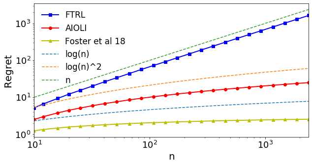
Refer to caption
Figure 2: Regret of each algorithm according to number of sample nn in log-log scale.

6 Conclusion and future work

To sum up, we designed a new efficient improper algorithm for online logistic regression. The latter only suffers logarithmic regret with much improved complexity compared to other existing methods. Some interesting questions are still remaining and left for future work.

Our online-to-batch procedure only provides upper-bounds in expectation. Obtaining high-probability bounds is more challenging and universal conversion methods such as the one of [Mehta, 2016] may not work for improper procedures.

Another interesting direction for future research is the extension to multi-class classification. Our analysis strongly relies on binary outputs to produce the improper regularization and the extension to multi-class is not straightforward. The next step would then be to extend the results to other settings considered by [Foster et al., 2018] such as bandit multi-class learning or online multi-class boosting. More generally, it would be interesting to study what are the class of functions where adaptive curvature parameters and improper learning yield to improved guarantees.

Finally, as shown in Section 4.1, AIOLI may be applied to nonparametric logistic regression in RKHS. However, without any approximation schemes, the computational complexity may become prohibitive of order O⁡(n3)O(n^{3}). Therefore, a possible line of research would be to study how much the performance of our algorithm would be affected by standard approximations techniques as Nyström projections or random features.

Acknowledgements

This work was funded in part by the French government under management of Agence Nationale de la Recherche as part of the "Investissements d’avenir" program, reference ANR-19-P3IA-0001 (PRAIRIE 3IA Institute).

References

  • [Aronszajn, 1950] Aronszajn, N. (1950). Theory of reproducing kernels. Transactions of the American mathematical society, 68(3):337–404.
  • [Azoury and Warmuth, 2001] Azoury, K. S. and Warmuth, M. K. (2001). Relative loss bounds for on-line density estimation with the exponential family of distributions. Machine Learning, 43(3):211–246.
  • [Berkson, 1944] Berkson, J. (1944). Application of the logistic function to bio-assay. Journal of the American statistical association, 39(227):357–365.
  • [Bubeck et al., 2018] Bubeck, S., Eldan, R., and Lehec, J. (2018). Sampling from a log-concave distribution with projected langevin monte carlo. Discrete & Computational Geometry, 59(4):757–783.
  • [Bubeck et al., 2015] Bubeck, S. et al. (2015). Convex optimization: Algorithms and complexity. Foundations and Trends® in Machine Learning, 8(3-4):231–357.
  • [Calandriello et al., 2017] Calandriello, D., Lazaric, A., and Valko, M. (2017). Efficient second-order online kernel learning with adaptive embedding. In Neural Information Processing Systems.
  • [Cesa-Bianchi and Lugosi, 2006] Cesa-Bianchi, N. and Lugosi, G. (2006). Prediction, learning, and games. Cambridge university press.
  • [Foster et al., 2018] Foster, D. J., Kale, S., Luo, H., Mohri, M., and Sridharan, K. (2018). Logistic regression: The importance of being improper. arXiv preprint arXiv:1803.09349.
  • [Gaillard et al., 2018] Gaillard, P., Gerchinovitz, S., Huard, M., and Stoltz, G. (2018). Uniform regret bounds over ℝd\mathbb{R}^{d} for the sequential linear regression problem with the square loss. arXiv preprint arXiv:1805.11386.
  • [Golub and Van Loan, 2012] Golub, G. H. and Van Loan, C. F. (2012). Matrix computations, volume 3. JHU press.
  • [Hazan et al., 2007] Hazan, E., Agarwal, A., and Kale, S. (2007). Logarithmic regret algorithms for online convex optimization. Machine Learning, 69(2-3):169–192.
  • [Hazan et al., 2016] Hazan, E. et al. (2016). Introduction to online convex optimization. Foundations and Trends® in Optimization, 2(3-4):157–325.
  • [Hazan et al., 2014] Hazan, E., Koren, T., and Levy, K. Y. (2014). Logistic regression: Tight bounds for stochastic and online optimization. In Conference on Learning Theory, pages 197–209.
  • [Helmbold and Warmuth, 1995] Helmbold, D. P. and Warmuth, M. K. (1995). On weak learning. Journal of Computer and System Sciences, 50(3):551–573.
  • [Jézéquel et al., 2019] Jézéquel, R., Gaillard, P., and Rudi, A. (2019). Efficient online learning with kernels for adversarial large scale problems. In Advances in Neural Information Processing Systems, pages 9427–9436.
  • [Marteau-Ferey et al., 2019] Marteau-Ferey, U., Ostrovskii, D., Bach, F., and Rudi, A. (2019). Beyond least-squares: Fast rates for regularized empirical risk minimization through self-concordance. arXiv preprint arXiv:1902.03046.
  • [McMahan, 2011] McMahan, H. B. (2011). Follow-the-regularized-leader and mirror descent: Equivalence theorems and l1 regularization. Journal of Machine Learning Research.
  • [Mehta, 2016] Mehta, N. A. (2016). Fast rates with high probability in exp-concave statistical learning. arXiv preprint arXiv:1605.01288.
  • [Mourtada and Gaïffas, 2019] Mourtada, J. and Gaïffas, S. (2019). An improper estimator with optimal excess risk in misspecified density estimation and logistic regression. arXiv preprint arXiv:1912.10784.
  • [Vovk, 1998] Vovk, V. (1998). A game of prediction with expert advice. Journal of Computer and System Sciences, 56(2):153–173.
  • [Vovk, 2001] Vovk, V. (2001). Competitive on-line statistics. International Statistical Review, 69(2):213–248.
  • [Zinkevich, 2003] Zinkevich, M. (2003). Online convex programming and generalized infinitesimal gradient ascent. In Proceedings of the 20th international conference on machine learning (icml-03), pages 928–936.

Appendix A Notation

In this section, we recall and define useful notations that will be used all along the proofs. At each round t⩾1t\geqslant 1, we recall that the forecaster is given an input xt∈𝒳⊂ℬ⁡(ℝd,R)x_{t}\in\mathcal{X}\subset\mathcal{B}(\mathbb{R}^{d},R); chooses a prediction θ^t∈ℝd\widehat{\theta}_{t}\in\mathbb{R}^{d}; forms the prediction y^t=θ^t⊤​xt\widehat{y}_{t}=\widehat{\theta}_{t}^{\top}x_{t}; and observes the outcome yt∈{−1,1}y_{t}\in\{-1,1\}. The loss of a parameter θ∈ℝd\theta\in\mathbb{R}^{d} at time t⩾1t\geqslant 1 is measured by ℓt​(θ)=ℓ⁡(θ⊤​xt,yt)=log⁡(1+e−yt​θ⊤​xt)\ell_{t}(\theta)=\ell(\theta^{\top}x_{t},y_{t})=\log(1+e^{-y_{t}\theta^{\top}x_{t}}).

We also define for all t⩾1t\geqslant 1, all θ∈ℝd\theta\in\mathbb{R}^{d} and y∈{−1,1}y\in\{-1,1\}:

  • -

    the loss suffered by θ\theta if the outcome was yy:   ℓty​(θ)=log⁡(1+e−y​θ⊤​xt)\ell_{t}^{y}(\theta)=\log(1+e^{-y\theta^{\top}x_{t}})

  • -

    the gradient of the loss in θ^t\widehat{\theta}_{t} if the outcome was yy:   gty=∇ℓty​(θ^t)g_{t}^{y}=\nabla\ell_{t}^{y}(\widehat{\theta}_{t})

  • -

    the curvature if the outcome was yy:   ηty=ey​θ^t⊤​xt1+B​R\eta_{t}^{y}=\frac{e^{y\widehat{\theta}_{t}^{\top}x_{t}}}{1+BR}

  • -

    the quadratic surrogate losses if the outcome was yy:
        ℓ^ty​(θ)=ℓty​(θ^t)+gty⊤​(θ−θ^t)+ηty2​(θ−θ^t)⊤​gty​gty⊤​(θ−θ^t)\widehat{\ell}_{t}^{y}(\theta)=\ell_{t}^{y}(\widehat{\theta}_{t})+g_{t}^{y\top}(\theta-\widehat{\theta}_{t})+\frac{\eta_{t}^{y}}{2}(\theta-\widehat{\theta}_{t})^{\top}g_{t}^{y}g_{t}^{y\top}(\theta-\widehat{\theta}_{t})

  • -

    the corresponding loss, surrogate loss, gradient, and curvature for the true outcome y^t\widehat{y}_{t}:
         ℓt=ℓtyt\ell_{t}=\ell_{t}^{y_{t}},  ℓ^t=ℓ^tyt\widehat{\ell}_{t}=\widehat{\ell}_{t}^{y_{t}}, gt=gtytg_{t}=g_{t}^{y_{t}}, ηt=ηtyt\eta_{t}=\eta_{t}^{y_{t}}

  • -

    the regularized cumulative loss and cumulative surrogate loss respectively:
         Lt​(θ)=∑s=1tℓs​(θ)+λ​‖θ‖2L_{t}(\theta)=\sum\limits_{s=1}^{t}\ell_{s}(\theta)+\lambda\|\theta\|^{2}, L^t​(θ)=∑s=1tℓ^s​(θ)+λ​‖θ‖2\widehat{L}_{t}(\theta)=\sum\limits_{s=1}^{t}\widehat{\ell}_{s}(\theta)+\lambda\|\theta\|^{2}

With these notations, we defined θt\theta_{t} and θ¯t\bar{\theta}_{t} as:

θt=argminθ∈ℝdL^t−1​(θ),andθ¯t=argminθ∈ℝd{L^t−1​(θ)+ℓt1​(θ)+ℓt−1​(θ)}.\theta_{t}=\mathop{\operatorname{argmin}}_{\theta\in\mathbb{R}^{d}}\widehat{L}_{t-1}(\theta)\,,\quad\text{and}\quad\bar{\theta}_{t}=\mathop{\operatorname{argmin}}_{\theta\in\mathbb{R}^{d}}\left\{\widehat{L}_{t-1}(\theta)+\ell_{t}^{1}(\theta)+\ell_{t}^{-1}(\theta)\right\}\,. (11)

Appendix B Proof of the main theorem

Theorem 7.

Let ε,λ,R>0\varepsilon,\lambda,R>0 and d,n⩾1d,n\geqslant 1. Let (x1,y1),…,(xn,yn)∈𝒳×𝒴(x_{1},y_{1}),...,(x_{n},y_{n})\in\mathcal{X}\times\mathcal{Y} be an arbitrary sequence of observations. Define θ¯t\bar{\theta}_{t} for t⩾1t\geqslant 1 as in Equation (11) with regularization parameter λ>0\lambda>0. Then, any estimator θ^t\widehat{\theta}_{t} which verifies for all t⩾1t\geqslant 1, ‖θ^t−θ¯t‖⩽ε\|\widehat{\theta}_{t}-\bar{\theta}_{t}\|\leqslant\varepsilon satisfies the following upper-bound on the regret

Rn​(θ)⩽λ​‖θ‖2+d⁡(1+B​R)​log⁡(1+n​R28​d​(1+B​R)​λ)+3​n​R​(n​R28​λ+B)​ε.R_{n}(\theta)\leqslant\lambda\|\theta\|^{2}+d(1+BR)\log\left(1+\frac{nR^{2}}{8d(1+BR)\lambda}\right)+3nR\left(\frac{nR^{2}}{8\lambda}+B\right)\varepsilon\,.

Proof Let θ∈ℬ⁡(ℝd,B)\theta\in\mathcal{B}(\mathbb{R}^{d},B). Let us first upper-bound the regret Rn​(θ)R_{n}(\theta) by the regret using the surrogate losses. Applying Lemma 5 with a=yt​θ⊤​xt∈[−B​R,B​R]a=y_{t}\theta^{\top}x_{t}\in[-BR,BR] and b∈yt​θ^t⊤​xt∈ℝb\in y_{t}\widehat{\theta}_{t}^{\top}x_{t}\in\mathbb{R}, we have for all t⩾1t\geqslant 1:

ℓt​(θ)⩾ℓ^t​(θ).\ell_{t}(\theta)\geqslant\widehat{\ell}_{t}(\theta).

Together with ℓt​(θ^t)=ℓ^t​(θ^t)\ell_{t}(\widehat{\theta}_{t})=\widehat{\ell}_{t}(\widehat{\theta}_{t}), it yields that the regret on the true loss is upper-bounded by the regret on the quadratic approximations

Rn​(θ)=∑t=1nℓt​(θ^t)−∑t=1nℓt​(θ)⩽∑t=1nℓ^t​(θ^t)−∑t=1nℓ^t​(θ)=R^n​(θ).\displaystyle R_{n}(\theta)=\sum\limits_{t=1}^{n}\ell_{t}(\widehat{\theta}_{t})-\sum\limits_{t=1}^{n}\ell_{t}(\theta)\leqslant\sum\limits_{t=1}^{n}\widehat{\ell}_{t}(\widehat{\theta}_{t})-\sum\limits_{t=1}^{n}\widehat{\ell}_{t}(\theta)=\widehat{R}_{n}(\theta)\,. (12)

Now, we are left with analyzing a quadratic problem. We can thus follow in the main lines the proof of [Gaillard et al., 2018] for online least squares. By definition of θn+1=argminθ∈ℝdL^n​(θ)\theta_{n+1}=\mathop{\operatorname{argmin}}_{\theta\in\mathbb{R}^{d}}\widehat{L}_{n}(\theta), L^n​(θn+1)⩽L^n​(θ)\widehat{L}_{n}(\theta_{n+1})\leqslant\widehat{L}_{n}(\theta), which can be written as

∑t=1nℓ^t​(θn+1)−∑t=1nℓ^t​(θ)\displaystyle\sum\limits_{t=1}^{n}\widehat{\ell}_{t}(\theta_{n+1})-\sum\limits_{t=1}^{n}\widehat{\ell}_{t}(\theta) ⩽λ​‖θ‖2−λ​‖θn+1‖2.\displaystyle\leqslant\lambda\|\theta\|^{2}-\lambda\|\theta_{n+1}\|^{2}\,.

Now, the regret can be upper-bounded as

R^n​(θ)\displaystyle\widehat{R}_{n}(\theta) ⩽λ​‖θ‖2+∑t=1nℓ^t​(θ^t)−∑t=1nℓ^t​(θn+1)−λ​‖θn+1‖2\displaystyle\leqslant\lambda\|\theta\|^{2}+\sum\limits_{t=1}^{n}\widehat{\ell}_{t}(\widehat{\theta}_{t})-\sum\limits_{t=1}^{n}\widehat{\ell}_{t}(\theta_{n+1})-\lambda\|\theta_{n+1}\|^{2}
=λ​‖θ‖2+∑t=1n[ℓ^t​(θ^t)+L^t−1​(θt)−L^t​(θt+1)].\displaystyle=\lambda\|\theta\|^{2}+\sum\limits_{t=1}^{n}\left[\widehat{\ell}_{t}(\widehat{\theta}_{t})+\widehat{L}_{t-1}(\theta_{t})-\widehat{L}_{t}(\theta_{t+1})\right]\,. (13)

With a little bit of abuse, we call the terms inside the sum on the right the instant regrets. Grouping the terms of same degrees in the quadratic approximation,

ℓ^t​(θ)\displaystyle\widehat{\ell}_{t}(\theta) =ℓt​(θ^t)+gt⊤​(θ−θ^t)+ηt2​(θ−θ^t)​gt​gt⊤​(θ−θ^t)\displaystyle=\ell_{t}(\widehat{\theta}_{t})+g_{t}^{\top}(\theta-\widehat{\theta}_{t})+\frac{\eta_{t}}{2}(\theta-\widehat{\theta}_{t})g_{t}g_{t}^{\top}(\theta-\widehat{\theta}_{t})
=ℓt​(θ^t)−gt⊤​θ^t+ηt2​θ^t⊤​gt​gt⊤​θ^t+gt⊤​θ−ηt​θ⊤​gt​gt⊤​θ^t+ηt2​θ⊤​gt​gt⊤​θ\displaystyle=\ell_{t}(\widehat{\theta}_{t})-g_{t}^{\top}\widehat{\theta}_{t}+\frac{\eta_{t}}{2}\widehat{\theta}_{t}^{\top}g_{t}g_{t}^{\top}\widehat{\theta}_{t}+g_{t}^{\top}\theta-\eta_{t}\theta^{\top}g_{t}g_{t}^{\top}\widehat{\theta}_{t}+\frac{\eta_{t}}{2}\theta^{\top}g_{t}g_{t}^{\top}\theta
=ct∗−2​bt∗⁣⊤​θ+ηt2​θ⊤​gt​gt⊤​θ\displaystyle=c_{t}^{*}-2b_{t}^{*\top}\theta+\frac{\eta_{t}}{2}\theta^{\top}g_{t}g_{t}^{\top}\theta

with ct∗=ℓt​(θ^t)−gt⊤​θ^t+ηt2​θ^t⊤​gt​gt⊤​θ^tc_{t}^{*}=\ell_{t}(\widehat{\theta}_{t})-g_{t}^{\top}\widehat{\theta}_{t}+\frac{\eta_{t}}{2}\widehat{\theta}_{t}^{\top}g_{t}g_{t}^{\top}\widehat{\theta}_{t} and bt∗=12​(−gt+ηt​(θ^t⊤​gt)​gt)b_{t}^{*}=\frac{1}{2}\big(-g_{t}+\eta_{t}(\widehat{\theta}_{t}^{\top}g_{t})g_{t}\big). Similarly, we can write the cumulative loss as

L^t​(θ)=∑s=1tcs∗⏟ct−2​(∑s=1tbs∗⏟bt)⊤​θ+θ⊤​(λ​I+∑s=1tηs2​gs​gs⊤⏟At)​θ.\widehat{L}_{t}(\theta)=\underbrace{\sum\limits_{s=1}^{t}c_{s}^{*}}_{c_{t}}-2\bigg(\underbrace{\sum\limits_{s=1}^{t}b_{s}^{*}}_{b_{t}}\bigg)^{\top}\theta+\theta^{\top}\bigg(\underbrace{\lambda I+\sum\limits_{s=1}^{t}\frac{\eta_{s}}{2}g_{s}g_{s}^{\top}}_{A_{t}}\bigg)\theta\,. (14)

The minimum of this quadratic, reached in θt+1=At−1​bt\theta_{t+1}=A_{t}^{-1}b_{t}, is

L^t​(θt+1)=ct−2​bt⊤​At−1⏟θt+1​At​θt+1+θt+1⊤​At​θt+1=ct−θt+1⊤​At​θt+1.\widehat{L}_{t}(\theta_{t+1})=c_{t}-2\underbrace{b_{t}^{\top}A_{t}^{-1}}_{\theta_{t+1}}A_{t}\theta_{t+1}+\theta_{t+1}^{\top}A_{t}\theta_{t+1}=c_{t}-\theta_{t+1}^{\top}A_{t}\theta_{t+1}\,.

We can write now the instant regret at tt as

ℓ^t​(θ^t)+L^t−1​(θt)−L^t​(θt+1)\displaystyle\widehat{\ell}_{t}(\widehat{\theta}_{t})+\widehat{L}_{t-1}(\theta_{t})-\widehat{L}_{t}(\theta_{t+1}) =ℓ^t​(θ^t)−ct∗+θt+1⊤​At​θt+1−θt⊤​At−1​θt\displaystyle=\widehat{\ell}_{t}(\widehat{\theta}_{t})-c_{t}^{*}+\theta_{t+1}^{\top}A_{t}\theta_{t+1}-\theta_{t}^{\top}A_{t-1}\theta_{t}
=gt⊤​θ^t−ηt2​θ^t⊤​gt​gt⊤​θ^t+θt+1⊤​At​θt+1−θt⊤​At−1​θt\displaystyle=g_{t}^{\top}\widehat{\theta}_{t}-\frac{\eta_{t}}{2}\widehat{\theta}_{t}^{\top}g_{t}g_{t}^{\top}\widehat{\theta}_{t}+\theta_{t+1}^{\top}A_{t}\theta_{t+1}-\theta_{t}^{\top}A_{t-1}\theta_{t}
=gt⊤​θ^t−θ^t⊤​(At−At−1)​θ^t+θt+1⊤​At​θt+1−θt⊤​At−1​θt.\displaystyle=g_{t}^{\top}\widehat{\theta}_{t}-\widehat{\theta}_{t}^{\top}(A_{t}-A_{t-1})\widehat{\theta}_{t}+\theta_{t+1}^{\top}A_{t}\theta_{t+1}-\theta_{t}^{\top}A_{t-1}\theta_{t}\,. (15)

The oracle θt+1\theta_{t+1} minimizes the quadratic function L^t\widehat{L}_{t} with Hessian 2​At2A_{t}. Thus, performing one newton step from θ^t\widehat{\theta}_{t} gives

θt+1\displaystyle\theta_{t+1} =θ^t−12At−1∇L^t(θ^t)\displaystyle=\widehat{\theta}_{t}-\frac{1}{2}A_{t}^{-1}\nabla\widehat{L}_{t}(\widehat{\theta}_{t})
=θ^t−12​At−1​[∇L^t−1​(θ^t)+gt]\displaystyle=\widehat{\theta}_{t}-\frac{1}{2}A_{t}^{-1}\left[\nabla\widehat{L}_{t-1}(\widehat{\theta}_{t})+g_{t}\right]
=θ^t+12​At−1​gt−yt−12​At−1​[∇L^t−1​(θ^t)+gt+gt−yt]\displaystyle=\widehat{\theta}_{t}+\frac{1}{2}A_{t}^{-1}g_{t}^{-y_{t}}-\frac{1}{2}A_{t}^{-1}\left[\nabla\widehat{L}_{t-1}(\widehat{\theta}_{t})+g_{t}+g_{t}^{-y_{t}}\right] (16)

Similarly, we have

θt\displaystyle\theta_{t} =θ^t−12At−1−1∇L^t−1(θ^t)\displaystyle=\widehat{\theta}_{t}-\frac{1}{2}A_{t-1}^{-1}\nabla\widehat{L}_{t-1}(\widehat{\theta}_{t})
=θ^t+12​At−1−1​(gt+gt−yt)−12​At−1−1​[∇L^t−1​(θ^t)+gt+gt−yt].\displaystyle=\widehat{\theta}_{t}+\frac{1}{2}A_{t-1}^{-1}(g_{t}+g_{t}^{-y_{t}})-\frac{1}{2}A_{t-1}^{-1}\left[\nabla\widehat{L}_{t-1}(\widehat{\theta}_{t})+g_{t}+g_{t}^{-y_{t}}\right]. (17)

Reorganizing the terms in the two previous equations leads to

gt\displaystyle g_{t} =2​[At​θ^t−At​θt+1−At−1​θ^t+At−1​θt].\displaystyle=2\left[A_{t}\widehat{\theta}_{t}-A_{t}\theta_{t+1}-A_{t-1}\widehat{\theta}_{t}+A_{t-1}\theta_{t}\right].

Substituting in the instant regret (15), this entails

ℓ^t​(θ^t)\displaystyle\widehat{\ell}_{t}(\widehat{\theta}_{t}) +L^t−1​(θt)−L^t​(θt+1)=2​θ^t⊤​At​θ^t−2​θt+1⊤​At​θ^t−2​θ^t⊤​At−1​θ^t+2​θt⊤​At−1​θ^t\displaystyle+\widehat{L}_{t-1}(\theta_{t})-\widehat{L}_{t}(\theta_{t+1})=2\widehat{\theta}_{t}^{\top}A_{t}\widehat{\theta}_{t}-2\theta_{t+1}^{\top}A_{t}\widehat{\theta}_{t}-2\widehat{\theta}_{t}^{\top}A_{t-1}\widehat{\theta}_{t}+2\theta_{t}^{\top}A_{t-1}\widehat{\theta}_{t}
−θ^t⊤​At​θ^t+θ^t⊤​At−1​θ^t+θt+1⊤​At​θt+1−θt⊤​At−1​θt\displaystyle\quad\quad-\widehat{\theta}_{t}^{\top}A_{t}\widehat{\theta}_{t}+\widehat{\theta}_{t}^{\top}A_{t-1}\widehat{\theta}_{t}+\theta_{t+1}^{\top}A_{t}\theta_{t+1}-\theta_{t}^{\top}A_{t-1}\theta_{t}
=θt+1⊤​At​θt+1−2​θt+1⊤​At​θ^t+θ^t⊤​At​θ^t−θt⊤​At−1​θt+2​θt⊤​At−1​θ^t−θ^t⊤​At−1​θ^t\displaystyle=\theta_{t+1}^{\top}A_{t}\theta_{t+1}-2\theta_{t+1}^{\top}A_{t}\widehat{\theta}_{t}+\widehat{\theta}_{t}^{\top}A_{t}\widehat{\theta}_{t}-\theta_{t}^{\top}A_{t-1}\theta_{t}+2\theta_{t}^{\top}A_{t-1}\widehat{\theta}_{t}-\widehat{\theta}_{t}^{\top}A_{t-1}\widehat{\theta}_{t}
=(θt+1−θ^t)⊤​At​(θt+1−θ^t)−(θt−θ^t)⊤​At−1​(θt−θ^t)\displaystyle=(\theta_{t+1}-\widehat{\theta}_{t})^{\top}A_{t}(\theta_{t+1}-\widehat{\theta}_{t})-(\theta_{t}-\widehat{\theta}_{t})^{\top}A_{t-1}(\theta_{t}-\widehat{\theta}_{t}) (18)

Rewriting equations (B) and (B), we have

2​At​(θt+1−θ^t)\displaystyle 2A_{t}(\theta_{t+1}-\widehat{\theta}_{t}) =gt−yt−δt\displaystyle=g_{t}^{-y_{t}}-\delta_{t}
2​At−1​(θt−θ^t)\displaystyle 2A_{t-1}(\theta_{t}-\widehat{\theta}_{t}) =gt−yt+gt−δt\displaystyle=g_{t}^{-y_{t}}+g_{t}-\delta_{t}

with δt=∇L^t−1​(θ^t)+gt+gt−yt\delta_{t}=\nabla\widehat{L}_{t-1}(\widehat{\theta}_{t})+g_{t}+g_{t}^{-y_{t}}.
Subtracting the first equation to the second, we can write the instant regret as a variance term and an optimization error term,

ℓ^t​(θ^t)+L^t−1​(θt)−L^t​(θt+1)=Zt+Ωt\widehat{\ell}_{t}(\widehat{\theta}_{t})+\widehat{L}_{t-1}(\theta_{t})-\widehat{L}_{t}(\theta_{t+1})=Z_{t}+\Omega_{t} (19)

where

Zt\displaystyle Z_{t} =14​gt−yt⊤​At−1​gt−yt−14​(gt+gt−yt)​At−1−1​(gt+gt−yt)\displaystyle=\frac{1}{4}g_{t}^{-y_{t}\top}A_{t}^{-1}g_{t}^{-y_{t}}-\frac{1}{4}(g_{t}+g_{t}^{-y_{t}})A_{t-1}^{-1}(g_{t}+g_{t}^{-y_{t}})

and

Ωt\displaystyle\Omega_{t} =14​[−2​gt−yt​At−1​δt+δt​At−1​δt+2​(gt+gt−yt)​At−1−1​δt−δt​At−1−1​δt].\displaystyle=\frac{1}{4}\left[-2g_{t}^{-y_{t}}A_{t}^{-1}\delta_{t}+\delta_{t}A_{t}^{-1}\delta_{t}+2(g_{t}+g_{t}^{-y_{t}})A_{t-1}^{-1}\delta_{t}-\delta_{t}A_{t-1}^{-1}\delta_{t}\right]\,.

B.1 Upper-bound of the variance term ZtZ_{t}

Let us focus on bounding the term ZtZ_{t}. Developing the terms and using the fact that At−1⩽AtA_{t-1}\leqslant A_{t}, we have

Zt\displaystyle Z_{t} =14​(gt+gt−yt−gt)⊤​At−1​(gt+gt−yt−gt)−14​(gt+gt−yt)⊤​At−1−1​(gt+gt−yt)\displaystyle=\frac{1}{4}(g_{t}+g_{t}^{-y_{t}}-g_{t})^{\top}A_{t}^{-1}(g_{t}+g_{t}^{-y_{t}}-g_{t})-\frac{1}{4}(g_{t}+g_{t}^{-y_{t}})^{\top}A_{t-1}^{-1}(g_{t}+g_{t}^{-y_{t}})
=14​gt⊤​At−1​gt−12​gt⊤​At−1​(gt+gt−yt)+14​(gt+gt−yt)⊤​At−1​(gt+gt−yt)\displaystyle=\frac{1}{4}g_{t}^{\top}A_{t}^{-1}g_{t}-\frac{1}{2}g_{t}^{\top}A_{t}^{-1}(g_{t}+g_{t}^{-y_{t}})+\frac{1}{4}(g_{t}+g_{t}^{-y_{t}})^{\top}A_{t}^{-1}(g_{t}+g_{t}^{-y_{t}})
−14​(gt+gt−yt)⊤​At−1−1​(gt+gt−yt)\displaystyle\quad-\frac{1}{4}(g_{t}+g_{t}^{-y_{t}})^{\top}A_{t-1}^{-1}(g_{t}+g_{t}^{-y_{t}})
⩽14​gt⊤​At−1​gt−12​gt⊤​At−1​(gt+gt−yt)\displaystyle\leqslant\frac{1}{4}g_{t}^{\top}A_{t}^{-1}g_{t}-\frac{1}{2}g_{t}^{\top}A_{t}^{-1}(g_{t}+g_{t}^{-y_{t}})
=−14​gt⊤​At−1​gt−12​gt⊤​At−1​gt−yt\displaystyle=-\frac{1}{4}g_{t}^{\top}A_{t}^{-1}g_{t}-\frac{1}{2}g_{t}^{\top}A_{t}^{-1}g_{t}^{-y_{t}}
⩽−12​gt⊤​At−1​gt−yt.\displaystyle\leqslant-\frac{1}{2}g_{t}^{\top}A_{t}^{-1}g_{t}^{-y_{t}}\,.

Using the definition of the logistic function, we can relate gtg_{t} and gt−ytg_{t}^{-y_{t}},

gt−yt=yt​xt1+e−yt​θ^t⊤​xt=eyt​θ^t⊤​xt​yt​xt1+eyt​θ^t⊤​xt=−(1+B​R)​ηt​gt,g_{t}^{-y_{t}}=\frac{y_{t}x_{t}}{1+e^{-y_{t}\widehat{\theta}_{t}^{\top}x_{t}}}=e^{y_{t}\widehat{\theta}_{t}^{\top}x_{t}}\frac{y_{t}x_{t}}{1+e^{y_{t}\widehat{\theta}_{t}^{\top}x_{t}}}=-(1+BR)\eta_{t}g_{t}\,, (20)

which implies,

Zt\displaystyle Z_{t} ⩽(1+B​R)​ηt2​gt⊤​At−1​gt.\displaystyle\leqslant(1+BR)\frac{\eta_{t}}{2}g_{t}^{\top}A_{t}^{-1}g_{t}\,.

Summing over t=1,…,nt=1,\dots,n, the sum telescopes thanks to Lemma 10, we obtain

∑t=1nZt⩽(1+B​R)​∑k=1dlog⁡(1+λk​(Cn)λ),\sum_{t=1}^{n}Z_{t}\leqslant(1+BR)\sum\limits_{k=1}^{d}\log\left(1+\frac{\lambda_{k}(C_{n})}{\lambda}\right)\,, (21)

where Cn=12​∑t=1nηt​gt​gt⊤C_{n}=\frac{1}{2}\sum_{t=1}^{n}\eta_{t}g_{t}g_{t}^{\top} and λk​(Cn)\lambda_{k}(C_{n}) is the kk largest eigenvalue of CnC_{n}.

Now to upper-bound the right-hand side we need to upper-bound the trace of CnC_{n}, which we do now. Recalling that gt=−ytxt/(1+exp(ytθ^t⊤xt))g_{t}=-y_{t}x_{t}/\big(1+\exp(y_{t}\widehat{\theta}_{t}^{\top}x_{t})\big), we have

ηt2​gt​gt⊤=12​(1+B​R)​ey​θ^t⊤​xt(1+eyt​θ^t⊤​xt)2​xt​xt⊤⩽18​(1+B​R)​xt​xt⊤,\frac{\eta_{t}}{2}g_{t}g_{t}^{\top}=\frac{1}{2(1+BR)}\frac{e^{y\widehat{\theta}_{t}^{\top}x_{t}}}{(1+e^{y_{t}\widehat{\theta}_{t}^{\top}x_{t}})^{2}}x_{t}x_{t}^{\top}\leqslant\frac{1}{8(1+BR)}x_{t}x_{t}^{\top}\,,

where for the inequality, we used that x/(1+x)2⩽1/4x/(1+x)^{2}\leqslant 1/4 for x⩾0x\geqslant 0. Therefore, Tr⁡(Cn)=∑k=1dλk​(Cn)⩽n​R2/(8​(1+B​R))\operatorname{Tr}(C_{n})=\sum_{k=1}^{d}\lambda_{k}(C_{n})\leqslant nR^{2}/(8(1+BR)) for all k⩾1k\geqslant 1. Now remark that the right-hand side of equation 21 is maximized under the constraint ∑k=1dλk​(Cn)⩽n​R2/(8​(1+B​R))\sum_{k=1}^{d}\lambda_{k}(C_{n})\leqslant nR^{2}/(8(1+BR)) when all the eigenvalues are equals i.e.,λk​(Cn)=n​R2/(8​d​(1+B​R))\lambda_{k}(C_{n})=nR^{2}/(8d(1+BR)) for all 1⩽k⩽d1\leqslant k\leqslant d which leads to

∑t=1nZt\displaystyle\sum_{t=1}^{n}Z_{t} ⩽d⁡(1+B​R)​log⁡(1+n​R28​d​(1+B​R)​λ)\displaystyle\leqslant d(1+BR)\log\left(1+\frac{nR^{2}}{8d(1+BR)\lambda}\right) (22)

B.2 Upper-bound on the optimization error Ωt\Omega_{t}

It remains to bound the the approximation term Ωt\Omega_{t}.

Ωt\displaystyle\Omega_{t} =14​[2​(gt+gt−yt)​At−1−1​δt−2​gt−yt​At−1​δt+δt​At−1​δt−δt​At−1−1​δt⏟⩽0]\displaystyle=\frac{1}{4}[2(g_{t}+g_{t}^{-y_{t}})A_{t-1}^{-1}\delta_{t}-2g_{t}^{-y_{t}}A_{t}^{-1}\delta_{t}+\underbrace{\delta_{t}A_{t}^{-1}\delta_{t}-\delta_{t}A_{t-1}^{-1}\delta_{t}}_{\leqslant 0}]
⩽12​λ​[2​‖gt−yt‖+‖gt‖]​‖δt‖\displaystyle\leqslant\frac{1}{2\lambda}\left[2\|g_{t}^{-y_{t}}\|+\|g_{t}\|\right]\|\delta_{t}\|
⩽3​R2​λ​‖δt‖.\displaystyle\leqslant\frac{3R}{2\lambda}\|\delta_{t}\|\,.

The last inequality is due to ‖gty‖⩽R\|g_{t}^{y}\|\leqslant R for all ‖xt‖⩽R\|x_{t}\|\leqslant R and y∈{−1,1}y\in\{-1,1\}. By definition of θ¯t∈argminθ∈ℝd{L^t−1​(θ)+ℓt​(θ)+ℓt−yt​(θ)}\bar{\theta}_{t}\in\mathop{\operatorname{argmin}}_{\theta\in\mathbb{R}^{d}}\left\{\widehat{L}_{t-1}(\theta)+\ell_{t}(\theta)+\ell_{t}^{-y_{t}}(\theta)\right\}, we have ∇L^t−1​(θ¯t)+∇ℓt​(θ¯t)+∇ℓt−yt​(θ¯t)=0\nabla\widehat{L}_{t-1}(\bar{\theta}_{t})+\nabla\ell_{t}(\bar{\theta}_{t})+\nabla\ell_{t}^{-y_{t}}(\bar{\theta}_{t})=0. Note also that gty=∇ℓty​(θ^t)g_{t}^{y}=\nabla\ell_{t}^{y}(\widehat{\theta}_{t}) for all y∈{−1,1}y\in\{-1,1\}. So δt\delta_{t} may be rewriten as

δt=∇L^t−1​(θ^t)+∇ℓt​(θ^t)+∇ℓt−yt​(θ^t)−∇L^t−1​(θ¯t)−∇ℓt​(θ¯t)−∇ℓt−yt​(θ¯t)\delta_{t}=\nabla\widehat{L}_{t-1}(\widehat{\theta}_{t})+\nabla\ell_{t}(\widehat{\theta}_{t})+\nabla\ell_{t}^{-y_{t}}(\widehat{\theta}_{t})-\nabla\widehat{L}_{t-1}(\bar{\theta}_{t})-\nabla\ell_{t}(\bar{\theta}_{t})-\nabla\ell_{t}^{-y_{t}}(\bar{\theta}_{t})

Using that ∇ℓt\nabla\ell_{t} and ∇ℓ^t\nabla\widehat{\ell}_{t} are R2/4R^{2}/4-Lipschitz (for ∇ℓ^t\nabla\widehat{\ell}_{t} remark that OPEN‖∇2ℓ^t​(θ)‖=‖ηt​gt​gt⊤‖⩽R2/4)\|\nabla^{2}\widehat{\ell}_{t}(\theta)\|=\|\eta_{t}g_{t}g_{t}^{\top}\|\leqslant R^{2}/4)), we have

‖δt‖\displaystyle\|\delta_{t}\| ⩽[(t+1)​R24+2​λ​B]​‖θ^t−θ^t‖.\displaystyle\leqslant\left[\frac{(t+1)R^{2}}{4}+2\lambda B\right]\|\widehat{\theta}_{t}-\widehat{\theta}_{t}\|\,. (23)

Summing over tt leads to

∑t=1nΩt⩽3​n​R​(n​R28​λ+B)​ε.\sum_{t=1}^{n}\Omega_{t}\leqslant 3nR\left(\frac{nR^{2}}{8\lambda}+B\right)\varepsilon\,. (24)

B.3 Conculsion of the proof

Using inequalities (12), (13) and (19), we have

Rn​(θ)⩽R^n​(θ)⩽λ​‖θ‖2+∑t=1nZt+∑t=1nΩtR_{n}(\theta)\leqslant\widehat{R}_{n}(\theta)\leqslant\lambda\|\theta\|^{2}+\sum_{t=1}^{n}Z_{t}+\sum_{t=1}^{n}\Omega_{t}

Finally, inequalities (21) and (24) concludes the proof. □\square

Appendix C Lemmas

Proof of Lemma 5. Let C>0C>0. First, note that for all x∈ℝx\in\mathbb{R}, f′​(x)=−(1+exp⁡(x))−1f^{\prime}(x)=-(1+\exp(x))^{-1}. To prove Lemma 5, we need to show that for α=(1+C)−1\alpha=(1+C)^{-1}, we have for all a∈[−C,C]a\in[-C,C] and b∈ℝb\in\mathbb{R}

log⁡(1+e−a)⩾log⁡(1+e−b)−11+eb​(a−b)+α2​eb(1+eb)2​(a−b)2.\log(1+e^{-a})\geqslant\log(1+e^{-b})-\frac{1}{1+e^{b}}(a-b)+\frac{\alpha}{2}\frac{e^{b}}{(1+e^{b})^{2}}(a-b)^{2}\,.

To do so, we fix b∈ℝb\in\mathbb{R} and we define the function ξ\xi as

ξ⁡(a)=log⁡(1+e−a)−log⁡(1+e−b)+11+eb​(a−b)−α2​eb(1+eb)2​(a−b)2,−C⩽a⩽C\xi(a)=\log(1+e^{-a})-\log(1+e^{-b})+\frac{1}{1+e^{b}}(a-b)-\frac{\alpha}{2}\frac{e^{b}}{(1+e^{b})^{2}}(a-b)^{2},\qquad-C\leqslant a\leqslant C

It remains to show that ξ\xi is non-negative on [−C,C][-C,C]. Because ξ⁡(b)=0\xi(b)=0, it suffices to prove

ξ′​(a)​{⩽0for​a⩽b⩾0for​a⩾b\xi^{\prime}(a)\begin{cases}\leqslant 0&\text{for}\ a\leqslant b\\ \geqslant 0&\text{for}\ a\geqslant b\end{cases} (25)

First, after some computation, differentiating ξ\xi leads to

ξ′​(a)=−11+ea+11+eb−α​eb(1+eb)2​(a−b),\xi^{\prime}(a)=-\frac{1}{1+e^{a}}+\frac{1}{1+e^{b}}-\frac{\alpha e^{b}}{(1+e^{b})^{2}}(a-b)\,,

which can also be rewritten as

ξ′​(a)=ea−eb(1+ea)​(1+eb)−α​eb(1+eb)2​(a−b).\xi^{\prime}(a)=\frac{e^{a}-e^{b}}{(1+e^{a})(1+e^{b})}-\alpha\frac{e^{b}}{(1+e^{b})^{2}}(a-b)\,.

Reorganizing the terms gives the following equation

(1+ea)​(1+eb)​e−b​ξ′​(a)=ea−b−1−α​1+ea1+eb​(a−b).(1+e^{a})(1+e^{b})e^{-b}\xi^{\prime}(a)=e^{a-b}-1-\alpha\frac{1+e^{a}}{1+e^{b}}(a-b)\,.

Therefore, (25) holds true as soon as

α⩽ea−b−1a−b​1+eb1+ea,\alpha\leqslant\frac{e^{a-b}-1}{a-b}\frac{1+e^{b}}{1+e^{a}}\,,

with the convention (e0−1)/0=1(e^{0}-1)/0=1. The latter is satisfied by Lemma 8, because α=(1+C)−1⩽(1+|a|)−1\alpha=(1+C)^{-1}\leqslant(1+|a|)^{-1} for all a∈[−C,C]a\in[-C,C]. □\square

Lemma 8.

For all a,b∈ℝa,b\in\mathbb{R},

11+|a|⩽ea−b−1a−b​1+eb1+ea.\frac{1}{1+|a|}\leqslant\frac{e^{a-b}-1}{a-b}\frac{1+e^{b}}{1+e^{a}}\,.

Proof Define the function h:ℝ2↦ℝh:\mathbb{R}^{2}\mapsto\mathbb{R} that corresponds to the right-hand side of the inequality

h⁡(a,b)=ea−b−1a−b​1+eb1+ea,(a,b)∈ℝ2.h(a,b)=\frac{e^{a-b}-1}{a-b}\frac{1+e^{b}}{1+e^{a}},\qquad(a,b)\in\mathbb{R}^{2}\,.

It is worth pointing out that even hh is normally not defined for a=ba=b, setting h⁡(a,a)=1h(a,a)=1 makes it well defined and infinitely differentiable on ℝ2\mathbb{R}^{2}.

Let a⩾ba\geqslant b. Then (1+eb)/(1+ea)⩾eb−a(1+e^{b})/(1+e^{a})\geqslant e^{b-a}, which implies

h⁡(a,b)⩾(ea−b−1)​eb−a(a−b)⩾eb−a−1b−a⩾11+a−b,h(a,b)\geqslant\frac{(e^{a-b}-1)e^{b-a}}{(a-b)}\geqslant\frac{e^{b-a}-1}{b-a}\geqslant\frac{1}{1+a-b}\,,

where the last inequality is because (ex−1)/x⩾(1−x)−1(e^{x}-1)/x\geqslant(1-x)^{-1} for all x⩽0x\leqslant 0.

Otherwise, let a⩽ba\leqslant b. Then (1+eb)/(1+ea)⩾1(1+e^{b})/(1+e^{a})\geqslant 1, which entails

h⁡(a,b)⩾ea−b−1(a−b)⩾11+b−ah(a,b)\geqslant\frac{e^{a-b}-1}{(a-b)}\geqslant\frac{1}{1+b-a}

Combining the two cases a⩽ba\leqslant b and a⩾ba\geqslant b together, we get

h⁡(a,b)⩾11+|a−b|.h(a,b)\geqslant\frac{1}{1+|a-b|}\,. (26)

Now we show that argminb∈ℝh⁡(a,b)\mathop{\operatorname{argmin}}_{b\in\mathbb{R}}h(a,b) contains a value between 00 and aa, i.e., in [0,a][0,a] if a⩾0a\geqslant 0 or in [a,0][a,0] otherwise. Rewriting the function hh as follows,

h⁡(a,b)\displaystyle h(a,b) =11+ea​ea−b−1a−b+11+e−a​eb−a−1b−a,\displaystyle=\frac{1}{1+e^{a}}\frac{e^{a-b}-1}{a-b}+\frac{1}{1+e^{-a}}\frac{e^{b-a}-1}{b-a}\,, (27)

it is clear that h⁡(a,b)=h⁡(−a,−b)h(a,b)=h(-a,-b). We can therefore suppose without loss of generality that aa is non-negative. Indeed, if b∗​(a)∈argminbh⁡(a,b)b^{*}(a)\in\mathop{\operatorname{argmin}}_{b}h(a,b) then −b∗​(a)∈argminbh⁡(−a,b)-b^{*}(a)\in\mathop{\operatorname{argmin}}_{b}h(-a,b). A further look at Equation (27) shows also that hh is convex in its second argument by convexity of the function x↦(ex−1)/xx\mapsto(e^{x}-1)/x and stability of convex functions by composition with affine transformations and non-negative weighted sum.

To finish the proof, we will show that the derivative of ∂h⁡(a,b)/∂b\partial h(a,b)/\partial b is non-negative for b→ab\to a and non-positive for b=0b=0. Convexity of hh in its second argument will then conclude. Using a⩾0a\geqslant 0, some computations (omitted here) lead to

∂∂b​h​(a,b)\displaystyle\frac{\partial}{\partial b}h(a,b) =(b−a+1)​ea−b−1+(b−a−1)​eb+ea(a−b)2​(1+ea).\displaystyle=\frac{(b-a+1)e^{a-b}-1+(b-a-1)e^{b}+e^{a}}{(a-b)^{2}(1+e^{a})}\,.

Develloping the first terms of the exponential series gives

(b−a+1)​ea−b−1+(b−a−1)​eb+ea=12​(ea−1)​(a−b)2+ob→a​((a−b)2).(b-a+1)e^{a-b}-1+(b-a-1)e^{b}+e^{a}=\frac{1}{2}(e^{a}-1)(a-b)^{2}+o_{b\to a}((a-b)^{2})\,.

Therefore,

limb→a∂∂b​h​(a,b)=12​ea−1ea+1⩾ 0.\lim_{b\rightarrow a}\frac{\partial}{\partial b}h(a,b)=\frac{1}{2}\frac{e^{a}-1}{e^{a}+1}\ \geqslant\ 0\,.

We note also that if a=0a=0 then ∂∂b​h​(0,0)=0\frac{\partial}{\partial b}h(0,0)=0. Now, if a>0a>0, using (2−x)​ex⩽2+x(2-x)e^{x}\leqslant 2+x for all x⩾0x\geqslant 0, we have

∂∂b​h​(a,0)=(2−a)​ea−(a+2)⩽0\frac{\partial}{\partial b}h(a,0)=(2-a)e^{a}-(a+2)\leqslant 0

By convexity of the function b↦h⁡(a,b)b\mapsto h(a,b), we conclude that argminb∈ℝh⁡(a,b)∈[0,a]\mathop{\operatorname{argmin}}_{b\in\mathbb{R}}h(a,b)\in[0,a]. Combined with Inequality (26) concludes the proof of the lemma. □\square

The following Lemma is a standard result of online matrix theory (Lemma 11.11 of [Cesa-Bianchi and Lugosi, 2006]).

Lemma 9.

Let V∈ℝd×dV\in\mathbb{R}^{d\times d} be an invertible matrix, u∈ℝdu\in\mathbb{R}^{d} and U=V−u​u⊤U=V-uu^{\top}. Then,

u⊤​V−1​u=1−det(U)det(V).u^{\top}V^{-1}u=1-\frac{\det(U)}{\det(V)}\,.
Lemma 10.

If Cn=∑t=1nηt2​gt​gt⊤C_{n}=\sum\limits_{t=1}^{n}\frac{\eta_{t}}{2}g_{t}g_{t}^{\top} and An=Cn+λ​IA_{n}=C_{n}+\lambda I then

∑t=1nηt2​gt⊤​At−1​gt⩽∑k=1dlog⁡(1+λk​(Cn)λ)\sum\limits_{t=1}^{n}\frac{\eta_{t}}{2}g_{t}^{\top}A_{t}^{-1}g_{t}\leqslant\sum\limits_{k=1}^{d}\log\left(1+\frac{\lambda_{k}(C_{n})}{\lambda}\right)

where λk​(Cn)\lambda_{k}(C_{n}) is the kk largest eigenvalue of CnC_{n}.

Proof Remarking that At=At−1+ηt2​gt​gt⊤A_{t}=A_{t-1}+\frac{\eta_{t}}{2}g_{t}g_{t}^{\top} and applying lemma 9 we have

ηt2​gt⊤​At−1​gt=1−det⁡(At−1/λ)det⁡(At/λ)\frac{\eta_{t}}{2}g_{t}^{\top}A_{t}^{-1}g_{t}=1-\frac{\operatorname{det}(A_{t-1}/\lambda)}{\operatorname{det}(A_{t}/\lambda)}

We use now that 1−u⩽log⁡(1/u)1-u\leqslant\log(1/u) for u>0u>0 which yields

ηt2​gt⊤​At−1​gt⩽log⁡det⁡(At/λ)det⁡(At−1/λ)\frac{\eta_{t}}{2}g_{t}^{\top}A_{t}^{-1}g_{t}\leqslant\log\frac{\operatorname{det}(A_{t}/\lambda)}{\operatorname{det}(A_{t-1}/\lambda)}

Summing over t=1,…,nt=1,...,n, using A0=λ​IA_{0}=\lambda I and An=Cn+λ​IA_{n}=C_{n}+\lambda I with Cn=∑t=1nηt2​gt​gt⊤C_{n}=\sum\limits_{t=1}^{n}\frac{\eta_{t}}{2}g_{t}g_{t}^{\top}, we get

∑t=1nηt2​gt⊤​At−1​gt\displaystyle\sum\limits_{t=1}^{n}\frac{\eta_{t}}{2}g_{t}^{\top}A_{t}^{-1}g_{t} ⩽log⁡(det⁡(I+Cnλ))\displaystyle\leqslant\log\left(\operatorname{det}\left(I+\frac{C_{n}}{\lambda}\right)\right)
=∑k=1dlog⁡(1+λk​(Cn)λ)\displaystyle=\sum\limits_{k=1}^{d}\log\left(1+\frac{\lambda_{k}(C_{n})}{\lambda}\right)

□\square

Appendix D Efficient implementation of AIOLI

L0=λ−1/2I,b~0=0,θ~0=0L_{0}=\lambda^{-1/2}I,\tilde{b}_{0}=0,\tilde{\theta}_{0}=0
for t=1,…,nt=1,...,n do
receives xtx_{t}
Wt=Lt−1​(bt−1,xt),{Ut,Σt}=eigen−dec⁡(Wt⊤​Wt),ut=Σt1/2​Ut⊤​e1,vt=Σt1/2​Ut⊤​e2W_{t}=L_{t}^{-1}(b_{t-1},x_{t}),~~\{U_{t},\Sigma_{t}\}=\operatorname{eigen-dec}(W_{t}^{\top}W_{t}),u_{t}=\Sigma_{t}^{1/2}U_{t}^{\top}e_{1},~~v_{t}=\Sigma_{t}^{1/2}U_{t}^{\top}e_{2}
ωt0=0\omega^{0}_{t}=0
for i=1,…,Ti=1,...,T do
    ωti=ωti−1−λ4​λ+R2​[2​ωti−1−2​ut−(1+evt⊤​ωti−1)−1​vt+(1+e−vt⊤​ωti−1)−1​vt]\omega^{i}_{t}=\omega^{i-1}_{t}-\frac{\lambda}{4\lambda+R^{2}}\left[2\omega^{i-1}_{t}-2u_{t}-(1+e^{v_{t}^{\top}\omega^{i-1}_{t}})^{-1}v_{t}+(1+e^{-v_{t}^{\top}\omega^{i-1}_{t}})^{-1}v_{t}\right] end for
   θ~t=Lt−⁣⊤(Wt(UtΣt−1/2ωtT))\tilde{\theta}_{t}=L_{t}^{-\top}(W_{t}(U_{t}\Sigma_{t}^{-1/2}\omega^{T}_{t}))
predict y^t=θ~t⊤​xt\widehat{y}_{t}=\tilde{\theta}_{t}^{\top}x_{t}
receives yty_{t}
gt=−(1+eyt​θ~t⊤​xt)−1​yt​xt,ηt=eyt​θ^t⊤​xt1+B​Rg_{t}=-(1+e^{y_{t}\tilde{\theta}_{t}^{\top}x_{t}})^{-1}y_{t}x_{t},\quad\eta_{t}=\frac{e^{y_{t}\widehat{\theta}_{t}^{\top}x_{t}}}{1+BR}
Lt=chol−update⁡(Lt−1,ηt/2​gt),bt=bt−1+(ηt​gt⊤​θ~t−1)​gtL_{t}=\operatorname{chol-update}(L_{t-1},\sqrt{\eta_{t}/2}g_{t}),\quad b_{t}=b_{t-1}+(\eta_{t}g_{t}^{\top}\tilde{\theta}_{t}-1)g_{t}
end for
Algorithm 2 AIOLI detailed version. Here eigen−dec\operatorname{eigen-dec} corresponds to economic-eigendecomposition of a symmetric matrix and chol−update\operatorname{chol-update} to the rank 1 Cholesky update [Golub and Van Loan, 2012]

Proof of Lemma 2 Given the definition of θ^t\widehat{\theta}_{t}, in (3), using the notation in Appendix A and Eq. (14)

θ^t\displaystyle\widehat{\theta}_{t} =argminθ∈ℝdL^t−1​(θ)+log⁡(1+e−θt⊤​xt)+log⁡(1+eθ⊤​xt)\displaystyle=~~\mathop{\operatorname{argmin}}_{\theta\in\mathbb{R}^{d}}~\widehat{L}_{t-1}(\theta)+\log(1+e^{-\theta_{t}^{\top}x_{t}})+\log(1+e^{\theta^{\top}x_{t}})
=argminθ∈ℝdθ⊤​At−1​θ−2​θ⊤​bt−1+log⁡(1+cosh⁡(θ⊤​xt)).\displaystyle=~~\mathop{\operatorname{argmin}}_{\theta\in\mathbb{R}^{d}}~\theta^{\top}A_{t-1}\theta-2\theta^{\top}b_{t-1}+\log(1+\operatorname{cosh}(\theta^{\top}x_{t})).

Since At−1A_{t-1} is invertible by construction and At−1=Lt−1​Lt−1⊤A_{t-1}=L_{t-1}L_{t-1}^{\top}, where Lt−1L_{t-1} is lower triangular and the unique Cholesky decomposition of At−1A_{t-1} [Golub and Van Loan, 2012], we can define the following equivalent problem, by the substitution r=Lt−1⊤​θr=L_{t-1}^{\top}\theta

rt=argminr∈ℝdr⊤​r−2​r⊤​u~t+log⁡(1+cosh⁡(r⊤​v~t)),u~t=Lt−1−1​bt−1,v~t=Lt−1−1​xt,r_{t}~~=~~\mathop{\operatorname{argmin}}_{r\in\mathbb{R}^{d}}~r^{\top}r-2r^{\top}\tilde{u}_{t}+\log(1+\operatorname{cosh}(r^{\top}\tilde{v}_{t})),\quad\tilde{u}_{t}=L_{t-1}^{-1}b_{t-1},\quad\tilde{v}_{t}=L_{t-1}^{-1}x_{t},

and in particular rt=Lt⊤​θ^tr_{t}=L_{t}^{\top}\widehat{\theta}_{t}. Now note that any r∈ℝdr\in\mathbb{R}^{d} can be always written as r=Wt​q+μr=W_{t}q+\mu with Wt=(u~t,v~t)∈ℝd×2W_{t}=(\tilde{u}_{t},\tilde{v}_{t})\in\mathbb{R}^{d\times 2} for some q∈ℝ2q\in\mathbb{R}^{2} and μ∈(span⁡Wt)⊥\mu\in(\operatorname{span}W_{t})^{\bot}, then rt=Wt​qt+μtr_{t}=W_{t}q_{t}+\mu_{t} for qt,μtq_{t},\mu_{t} defined as

(qt,μt)\displaystyle(q_{t},\mu_{t}) =argminq∈ℝ2,μ∈(span⁡Wt)⊥‖Wt​q+μ‖2−2​u~t⊤​(Wt​q+μ)+log⁡(1+cosh⁡(v~t⊤​(Wt​q+μ)))\displaystyle=\mathop{\operatorname{argmin}}_{q\in\mathbb{R}^{2},\mu\in(\operatorname{span}W_{t})^{\bot}}\|W_{t}q+\mu\|^{2}-2\tilde{u}_{t}^{\top}(W_{t}q+\mu)+\log(1+\operatorname{cosh}(\tilde{v}_{t}^{\top}(W_{t}q+\mu)))
=argminq∈ℝ2,μ∈(span⁡Wt)⊥‖Wt​q‖2+‖μ‖2−2​u~t⊤​Wt​q+log⁡(1+cosh⁡(v~t⊤​Wt​q)),\displaystyle=\mathop{\operatorname{argmin}}_{q\in\mathbb{R}^{2},\mu\in(\operatorname{span}W_{t})^{\bot}}\|W_{t}q\|^{2}+\|\mu\|^{2}-2\tilde{u}_{t}^{\top}W_{t}q+\log(1+\operatorname{cosh}(\tilde{v}_{t}^{\top}W_{t}q)),

where in the last inequality we use the fact that u~t=Wt​e1\tilde{u}_{t}=W_{t}e_{1}, v~t=Wt​e2\tilde{v}_{t}=W_{t}e_{2} and Wt⊤​μ=0W_{t}^{\top}\mu=0, by construction. Now the solution of the problem above is given by μt=0\mu_{t}=0 and qtq_{t} as

qt=argminq∈ℝ2‖Wt​q‖2−2​u~t⊤​Wt​q+log⁡(1+cosh⁡(v~t⊤​Wt​q)).q_{t}~~=~~\mathop{\operatorname{argmin}}_{q\in\mathbb{R}^{2}}~\|W_{t}q\|^{2}-2\tilde{u}_{t}^{\top}W_{t}q+\log(1+\operatorname{cosh}(\tilde{v}_{t}^{\top}W_{t}q)).

Now that in the problem above qq is always applied to WtW_{t}, so in the case that WtW_{t} is not full rank then all the solutions of the form qt=qt0+ζq_{t}=q^{0}_{t}+\zeta with ζ∈(span⁡Wt⊤​Wt)⊥\zeta\in(\operatorname{span}W_{t}^{\top}W_{t})^{\bot} are admissible and leading to the same rtr_{t}. Then we can restrict the problem above as

qt=argminq∈span⁡Wt⊤​Wt‖Wt​q‖2−2​u~t⊤​Wt​q+log⁡(1+cosh⁡(v~t⊤​Wt​q)).q_{t}~~=~~\mathop{\operatorname{argmin}}_{q\in\operatorname{span}W_{t}^{\top}W_{t}}~\|W_{t}q\|^{2}-2\tilde{u}_{t}^{\top}W_{t}q+\log(1+\operatorname{cosh}(\tilde{v}_{t}^{\top}W_{t}q)).

To conclude, take the economic eigenvalue decomposition of Wt⊤​WtW_{t}^{\top}W_{t}, i.e., Wt⊤​Wt=Ut​Σt​Ut⊤W_{t}^{\top}W_{t}=U_{t}\Sigma_{t}U_{t}^{\top} with Ut∈ℝ2×ptU_{t}\in\mathbb{R}^{2\times p_{t}} with ptp_{t} the rank of Wt⊤​WtW_{t}^{\top}W_{t}, such that Ut⊤​Ut=IU_{t}^{\top}U_{t}=I and Σt∈ℝpt×pt\Sigma_{t}\in\mathbb{R}^{p_{t}\times p_{t}} is diagonal and positive [Golub and Van Loan, 2012]. Now we consider the substitution ω=Σt1/2​Ut⊤​q\omega=\Sigma_{t}^{1/2}U_{t}^{\top}q, whose inverse is q=UtΣt−1/2ωq=U_{t}\Sigma_{t}^{-1/2}\omega since q∈span⁡Wt⊤​Wtq\in\operatorname{span}W_{t}^{\top}W_{t} and Ut​Ut⊤U_{t}U_{t}^{\top} is the projection matrix whose span is exactly span⁡Wt⊤​Wt\operatorname{span}W_{t}^{\top}W_{t}, i. e. Ut​Ut⊤​q=qU_{t}U_{t}^{\top}q=q for any q∈span⁡Wt⊤​Wtq\in\operatorname{span}W_{t}^{\top}W_{t}, which leads to the equivalent problem

ωt=argminω∈ℝptω⊤​ω−2​ut⊤​ω+log⁡(1+cosh⁡(vt⊤​ω)),\omega_{t}~~=~~\mathop{\operatorname{argmin}}_{\omega\in\mathbb{R}^{p_{t}}}~\omega^{\top}\omega-2u_{t}^{\top}\omega+\log(1+\operatorname{cosh}(v_{t}^{\top}\omega)),

where

ut\displaystyle u_{t} =Σt−1/2Ut⊤Wt⊤u~t=Σt−1/2Ut⊤Wt⊤Wte1=Σt1/2Ut⊤e1,\displaystyle=\Sigma_{t}^{-1/2}U_{t}^{\top}W_{t}^{\top}\tilde{u}_{t}=\Sigma_{t}^{-1/2}U_{t}^{\top}W_{t}^{\top}W_{t}e_{1}=\Sigma_{t}^{1/2}U_{t}^{\top}e_{1},
vt\displaystyle v_{t} =Σt−1/2Ut⊤Wt⊤v~t=Σt−1/2Ut⊤Wt⊤Wte2=Σt1/2Ut⊤e2.\displaystyle=\Sigma_{t}^{-1/2}U_{t}^{\top}W_{t}^{\top}\tilde{v}_{t}=\Sigma_{t}^{-1/2}U_{t}^{\top}W_{t}^{\top}W_{t}e_{2}=\Sigma_{t}^{1/2}U_{t}^{\top}e_{2}.

Note that in particular ωt=Σt1/2​Ut​qt\omega_{t}=\Sigma_{t}^{1/2}U_{t}q_{t} and qt=UtΣt−1/2ωtq_{t}=U_{t}\Sigma_{t}^{-1/2}\omega_{t}. Then

θ^t=Lt−1−⁣⊤rt=Lt−1−⁣⊤Wtqt=Lt−1−⁣⊤WtUtΣt−1/2ωt.\widehat{\theta}_{t}=L_{t-1}^{-\top}r_{t}=L_{t-1}^{-\top}W_{t}q_{t}=L_{t-1}^{-\top}W_{t}U_{t}\Sigma_{t}^{-1/2}\omega_{t}.

□\square

Proof of Lemma 3 Since Ωt\Omega_{t} is smooth and strongly convex, we can apply standard results on gradient descent (see for example Theorem 3.10 of [Bubeck et al., 2015]), obtaining

∥ωTt−ωt∥⩽e−T/(2κt)∥ω0t−ωt∥,\|\omega^{T}_{t}-\omega_{t}\|\leqslant e^{-T/(2\kappa_{t})}\|\omega^{0}_{t}-\omega_{t}\|,

when gradient descent is used with step-size γ=1/βt\gamma=1/\beta_{t} and where κt=βt/αt\kappa_{t}=\beta_{t}/\alpha_{t} with αt\alpha_{t} a lower bound of the strong convexity constant of Ωt\Omega_{t} and βt\beta_{t} an upper bound the Lipschitz constant of ∇Ωt\nabla\Omega_{t}. Note indeed that if Ωt\Omega_{t} is α\alpha-strongly convex for some α\alpha, it will be also α′\alpha^{\prime}-strongly convex, for any 0<α′⩽α0<\alpha^{\prime}\leqslant\alpha; moreover if ∇Ωt\nabla\Omega_{t} is β\beta-Lipschitz for some β\beta, it will be also β′\beta^{\prime}-Lipschitz, for any β′⩾β\beta^{\prime}\geqslant\beta; for more details see Chapter 3.4 of [Bubeck et al., 2015]. Now, by construction αt=1\alpha_{t}=1, indeed Ωt​(ω)−‖ω‖2\Omega_{t}(\omega)-\|\omega\|^{2} is still a convex problem. Moreover, for any ω,ω′∈ℝ2\omega,\omega^{\prime}\in\mathbb{R}^{2}, by the mean value theorem applied to the function g:[0,1]→ℝ2g:[0,1]\to\mathbb{R}^{2} defined as g⁡(r)=∇Ω​(ω+r⁡(ω′−ω))g(r)=\nabla\Omega(\omega+r(\omega^{\prime}-\omega)), there exists a q∈ℝ2q\in\mathbb{R}^{2} such that

∇Ωt​(ω)−∇Ωt​(ω′)=∇2Ωt​(q)​(ω′−ω).\nabla\Omega_{t}(\omega)-\nabla\Omega_{t}(\omega^{\prime})=\nabla^{2}\Omega_{t}(q)(\omega^{\prime}-\omega).

This implies that ‖∇Ωt​(ω)−∇Ωt​(ω′)‖⩽supq‖∇2Ωt​(q)‖​‖ω′−ω‖\|\nabla\Omega_{t}(\omega)-\nabla\Omega_{t}(\omega^{\prime})\|\leqslant\sup_{q}\|\nabla^{2}\Omega_{t}(q)\|\|\omega^{\prime}-\omega\| so the Lipschitz constant of ∇Ωt\nabla\Omega_{t} is upper bounded by βt=supq‖∇2Ωt​(q)‖\beta_{t}=\sup_{q}\|\nabla^{2}\Omega_{t}(q)\|. The Hessian of Ωt\Omega_{t} is defined as

∇2Ωt​(ω)=2​I+11+cosh⁡(vt⊤​ω)​vt​vt⊤,\nabla^{2}\Omega_{t}(\omega)=2I+\frac{1}{1+\cosh(v_{t}^{\top}\omega)}v_{t}v_{t}^{\top},

then

supq‖∇2Ωt​(q)‖⩽2+‖vt‖2​supw11+cosh⁡(vt⊤​w)⩽2+‖vt‖22.\sup_{q}\|\nabla^{2}\Omega_{t}(q)\|\leqslant 2+\|v_{t}\|^{2}\sup_{w}\frac{1}{1+\cosh(v_{t}^{\top}w)}\leqslant 2+\frac{\|v_{t}\|^{2}}{2}.

To conclude, note that vtv_{t} in Thm. 2 is defined as vt=(Wt⊤​Wt)1/2​e2v_{t}=(W_{t}^{\top}W_{t})^{1/2}e_{2} with e2=(0,1)e_{2}=(0,1), Wt=Lt−1−1​(bt−1,xt)W_{t}=L_{t-1}^{-1}(b_{t-1},x_{t}), Lt−1L_{t-1} the lower triangular Cholesky decomposition of At−1A_{t-1} (i.e. At−1=Lt−1​Lt−1⊤A_{t-1}=L_{t-1}L_{t-1}^{\top}) and At−1,bt−1A_{t-1},b_{t-1} defined in Eq. (5). Then

‖vt‖2=vt⊤​vt=e2​Ut​Σt​Ut⊤​e2⊤=e2​Wt⊤​Wt​e2=xt⊤​Lt−1−⁣⊤​Lt−1−1​xt=xt⊤​At−1−1​xt.\|v_{t}\|^{2}=v_{t}^{\top}v_{t}=e_{2}U_{t}\Sigma_{t}U_{t}^{\top}e_{2}^{\top}=e_{2}W_{t}^{\top}W_{t}e_{2}=x_{t}^{\top}L_{t-1}^{-\top}L_{t-1}^{-1}x_{t}=x_{t}^{\top}A_{t-1}^{-1}x_{t}.

So ‖vt‖2⩽‖xt‖2​‖At−1‖−1⩽R2/λ\|v_{t}\|^{2}\leqslant\|x_{t}\|^{2}\|A_{t-1}\|^{-1}\leqslant R^{2}/\lambda, since ‖xt‖⩽R\|x_{t}\|\leqslant R by assumption and At−1⪰λ​IA_{t-1}\succeq\lambda I by construction. Finally βt=2+‖vt‖2/2⩽2+R2/(2​λ)\beta_{t}=2+\|v_{t}\|^{2}/2\leqslant 2+R^{2}/(2\lambda) and αt=1\alpha_{t}=1, then κt⩽2+R2/(2​λ)\kappa_{t}\leqslant 2+R^{2}/(2\lambda) and γt=1/(2+R2/(2​λ))\gamma_{t}=1/(2+R^{2}/(2\lambda)). We have

∥ωtT−ωt∥⩽exp(−T/(2κt)+log∥)⩽exp(−T/(4+R2/λ)+log∥ωt0−ωt∥).\|\omega^{T}_{t}-\omega_{t}\|\leqslant\exp(-T/(2\kappa_{t})+\log\|)\leqslant\exp(-T/(4+R^{2}/\lambda)+\log\|\omega^{0}_{t}-\omega_{t}\|).

To quantify ‖ωt0−ωt‖\|\omega^{0}_{t}-\omega_{t}\| we need a bound for ‖ωt‖\|\omega_{t}\|. Note that, since Ωt\Omega_{t} is smooth and convex, ωt\omega_{t} is characterized by ∇Ωt​(ωt)=0\nabla\Omega_{t}(\omega_{t})=0, i.e. 2​ωt−2​ut−(1+evt⊤​ωt)−1​vt+(1+e−vt⊤​ωt)−1​vt=02\omega_{t}-2u_{t}-(1+e^{v_{t}^{\top}\omega_{t}})^{-1}v_{t}+(1+e^{-v_{t}^{\top}\omega_{t}})^{-1}v_{t}=0, from which

‖ωt‖⩽‖ut‖+supq|(1+e−vt⊤​q)−1−(1+evt⊤​q)−1|​‖vt‖/2⩽‖ut‖+‖vt‖/2.\|\omega_{t}\|\leqslant\|u_{t}\|+\sup_{q}\left|(1+e^{-v_{t}^{\top}q})^{-1}-(1+e^{v_{t}^{\top}q})^{-1}\right|\|v_{t}\|/2\leqslant\|u_{t}\|+\|v_{t}\|/2.

Analogously to the case of vtv_{t}, by definition of utu_{t}, we have ‖ut‖2=e1​Wt⊤​Wt​e1=bt−1​At−1−1​bt−1,\|u_{t}\|^{2}=e_{1}W_{t}^{\top}W_{t}e_{1}=b_{t-1}A_{t-1}^{-1}b_{t-1}, then ‖ut‖2⩽‖bt−1‖2​‖At−1−1‖⩽‖bt−1‖2/λ\|u_{t}\|^{2}\leqslant\|b_{t-1}\|^{2}\|A_{t-1}^{-1}\|\leqslant\|b_{t-1}\|^{2}/\lambda. Now we need a bound for bt−1b_{t-1}. Note that for any s∈{1,…,t−1}s\in\{1,\dots,t-1\}, we have gs=∇ℓs​(θ^s)=−(1+eys​θ^s⊤​xs)−1​ys​xsg_{s}=\nabla\ell_{s}(\widehat{\theta}_{s})=-(1+e^{y_{s}\widehat{\theta}_{s}^{\top}x_{s}})^{-1}y_{s}x_{s}, moreover ηs=eys​θ^s⊤​xs/(1+B​R)\eta_{s}=e^{y_{s}\widehat{\theta}_{s}^{\top}x_{s}}/(1+BR) and

(ηs​gs⊤​θ^s−1)​gs=ys​xs⊤​θ^s2+2​cosh⁡(ys​xs⊤​θ^s)​(1+B​R)−1​ys​xs+11+eys​xs⊤​θ^s​ys​xs.(\eta_{s}g_{s}^{\top}\widehat{\theta}_{s}-1)g_{s}=\frac{y_{s}x_{s}^{\top}\widehat{\theta}_{s}}{2+2\cosh(y_{s}x_{s}^{\top}\widehat{\theta}_{s})}(1+BR)^{-1}y_{s}x_{s}+\frac{1}{1+e^{y_{s}x_{s}^{\top}\widehat{\theta}_{s}}}y_{s}x_{s}.

Since supz|z/(2+2​cosh⁡(z))|⩽1\sup_{z}|z/(2+2\cosh(z))|\leqslant 1, ys∈{−1,1}y_{s}\in\{-1,1\} and ‖xs‖⩽R\|x_{s}\|\leqslant R by assumption, we have ‖(ηs​gs⊤​θ^s−1)​gs‖⩽((1+B​R)−1+1)​R⩽2​R\|(\eta_{s}g_{s}^{\top}\widehat{\theta}_{s}-1)g_{s}\|\leqslant((1+BR)^{-1}+1)R\leqslant 2R, then

‖bt−1‖=12​∑s=1t−1‖(ηs​gs⊤​θ^s−1)​gs‖⩽(t−1)​R.\|b_{t-1}\|=\frac{1}{2}\sum_{s=1}^{t-1}\|(\eta_{s}g_{s}^{\top}\widehat{\theta}_{s}-1)g_{s}\|\leqslant(t-1)R. (28)

To conclude, ∥ut∥⩽Rλ−1/2(t−1)\|u_{t}\|\leqslant R\lambda^{-1/2}(t-1), ∥ωt∥⩽∥ut∥+∥vt∥/2⩽Rλ−1/2t\|\omega_{t}\|\leqslant\|u_{t}\|+\|v_{t}\|/2\leqslant R\lambda^{-1/2}t. By choosing ωt0=0\omega^{0}_{t}=0, then Pt=∥ωt∥⩽Rλ−1/2tP_{t}=\|\omega_{t}\|\leqslant R\lambda^{-1/2}t and so ‖ωtT−ωt‖⩽ε\|\omega^{T}_{t}-\omega_{t}\|\leqslant\varepsilon, when choosing T⩾(4+R2/λ)log(Rλ−1/2t/ε)T\geqslant(4+R^{2}/\lambda)\log(R\lambda^{-1/2}t/\varepsilon). □\square

Proof of Theorem 4 We first analyze the cost of one iteration of Algorithm 1 (which is detailed in Algorithm 2 presented above). Note that at each step tt, the cost of the gradient descent algorithm performed to compute ωtT\omega^{T}_{t} is the number of iterations TT, since we are solving a ptp_{t}-dimensional problem, with pt∈{1,2}p_{t}\in\{1,2\}. The two most expensive operation performed at step tt (excluding gradient descent) are the solution of triangular linear systems of dimensions d×dd\times d when computing Lt−1−1​vL_{t-1}^{-1}v or Lt−1−⁣⊤​vL_{t-1}^{-\top}v for some vector v∈ℝdv\in\mathbb{R}^{d}, which costs O⁡(d2)O(d^{2}) (this operation is performed 4 times). The other expensive operation is the rank 1 Cholesky update of Lt−1L_{t-1} with the vector ηt/2​gt\sqrt{\eta_{t}/2}g_{t}, which costs O⁡(d2)O(d^{2}) [Golub and Van Loan, 2012], indeed the eigendecomposition is performed on the matrix Wt⊤​WtW_{t}^{\top}W_{t} which is 2×22\times 2. By repeating such operation for nn steps, we obtain a total cost of

O⁡(n​d2+n​T).O(nd^{2}+nT).

The upper-bound on the regret is a direct consequence of Theorem 7 and Lemma 3, with TT chosen according to the lemma and ε=λ3​n​R​(n​R28​λ+B)\varepsilon=\frac{\sqrt{\lambda}}{3nR\left(\frac{nR^{2}}{8\lambda}+B\right)}, since ‖Lt−1−1‖2=‖At−1−1‖⩽λ−1\|L_{t-1}^{-1}\|^{2}=\|A_{t-1}^{-1}\|\leqslant\lambda^{-1} and WtUtΣt−1/2W_{t}U_{t}\Sigma_{t}^{-1/2} is a partial isometry, we have

∥θ^t−θ~t∥⩽∥Lt−1−1∥∥WtUtΣt−1/2∥∥ωt−ωtT∥⩽λ−1/2ε⩽13​n​R​(n​R28​λ+B),\|\widehat{\theta}_{t}-\tilde{\theta}_{t}\|\leqslant\|L_{t-1}^{-1}\|\|W_{t}U_{t}\Sigma_{t}^{-1/2}\|\|\omega_{t}-\omega_{t}^{T}\|\leqslant\lambda^{-1/2}\varepsilon\leqslant\frac{1}{3nR\left(\frac{nR^{2}}{8\lambda}+B\right)}, (29)

that plugged in the result of Theorem 7 gives the desired result.

□\square