Differential Treatment for Stuff and Things:
A Simple Unsupervised Domain Adaptation Method for Semantic Segmentation

Zhonghao Wang Mo Yu Yunchao Wei Rogerio Feris Jinjun Xiong Wen-mei Hwu Thomas S. Huang Humphrey Shi Affiliation: C3SR, UIUC, IBM Research, ReLER, UTS, University of Oregon

Abstract

We consider the problem of unsupervised domain adaptation for semantic segmentation by easing the domain shift between the source domain (synthetic data) and the target domain (real data) in this work. State-of-the-art approaches prove that performing semantic-level alignment is helpful in tackling the domain shift issue. Based on the observation that stuff categories usually share similar appearances across images of different domains while things (i.e. object instances) have much larger differences, we propose to improve the semantic-level alignment with different strategies for stuff regions and for things: 1) for the stuff categories, we generate feature representation for each class and conduct the alignment operation from the target domain to the source domain; 2) for the thing categories, we generate feature representation for each individual instance and encourage the instance in the target domain to align with the most similar one in the source domain. In this way, the individual differences within thing categories will also be considered to alleviate over-alignment. In addition to our proposed method, we further reveal the reason why the current adversarial loss is often unstable in minimizing the distribution discrepancy and show that our method can help ease this issue by minimizing the most similar stuff and instance features between the source and the target domains. We conduct extensive experiments in two unsupervised domain adaptation tasks, i.e. GTA5 $\rightarrow$ Cityscapes and SYNTHIA $\rightarrow$ Cityscapes, and achieve the new state-of-the-art segmentation accuracy. Our code will be avaiable at https://github.com/SHI-Labs/Unsupervised-Domain-Adaptation-with-Differential-Treatment.

Refer to caption — Figure 1: Illustration of the proposed Stuff Instance Matching (SIM) structure. By matching the most similar stuff regions and things (i.e., instances) with differential treatment, we can adapt the features more accurately from the source domain to the target domain.

1 Introduction

Semantic segmentation Long_2015_CVPR enables image scene understanding at the pixel level, which is crucial to many real-world applications such as autonomous driving. The recent surge of deep learning deeplearning methods that generate features from large training datasets has significantly accelerated the progress in semantic segmentation deeplabv1; deeplabv2; pspnet; deeplabv3; huang2019ccnet; huang2020alignseg; cheng2019spgnet; wei2018revisiting; 2019arXiv191110194C; jiao2019geometry; qian2019weakly. However, collecting data with pixel-level annotation is costly in terms of both time and money. Specifically, to annotate an image in the widely used benchmark Cityscapes cityscapes takes 1.5 hours on average; that sums up to 7,500 hours in total for annotating all the 5,000 images. Such annotation cost is quite burdensome, given that training deep neural networks on the collected data usually takes less than dozens of hours.

To address the problem of high-cost annotation, unsupervised domain adaptation methods are proposed for semantic segmentation gta; synthia. In these works, a model trained on a source domain dataset with segmentation annotations is adapted for an unlabeled target domain. The source domain datasets can be synthetic, e.g., from video games, so that little human effort is required. However, such methods suffer from the domain shift problem. Existing methods deal with the problem by minimizing the distribution discrepancy of the features extracted by a feature extractor vgg; resnet between the source domain and the target domain. To this end, the GAN gan architectures, usually composed of a generator and a discriminator, are broadly used in this context. The generator extracts features from the input images, and the discriminator distinguishes which domain the features are generated from. The discriminator can thereby guide the generator to generate the target domain features with a distribution closer to the feature distribution of the source domain in an adversarial way.

In the previous GAN-style approaches, the adversarial loss is essentially a binary cross-entropy about whether the generated feature is from the source domain. We observe that such a global training signal is usually weak for the segmentation task. First, the alignments between stuff regions and between things require different treatments but the adversarial loss lacks such structural information. For example, the stuff regions usually lack the appearance variance in an image but the things can have diverse appearances in the same image. Therefore, it is sub-optimal to use an adversarial loss to align the stuff and thing features globally without differential treatments. Second, the global GAN structure only adapts the feature distribution between two domains and does not necessarily adapt the target domain features towards the most likely space of source domain features. Therefore, as the semantic head gathers the features from the source domain with more training iterations, it becomes harder for the feature generator to adapt the target domain features exactly toward the source domain features. This leads to a performance drop on the target domain images as shown in figure 2.

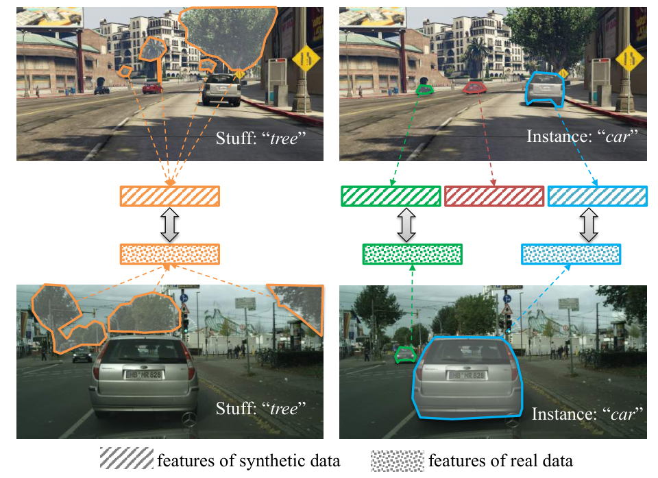
This paper proposes a stuff and instance matching (SIM) framework to address the aforementioned difficulties. First, we treat the alignments between stuff regions and between instances of things with different guidance. The key idea is shown in figure 1. The multiple stuff regions in a source image are usually similar, so the stuff from different domains can be directly aligned with their global feature vectors. While the multiple instances of the same thing, e.g., of the car category, can be diverse in the source image. Therefore we align instances in the target image to the most similar ones in the source image.

Second, we deal with the instability with the GAN training framework, we apply a L1 loss to explicitly minimize the distance between the target domain stuff and thing features with the most similar source domain counterparts. In this way, the adaptation is processed in a more accurate direction, instead of the rough distribution matching when using only the adversarial cross entropy loss, even after the semantic head gathers the source domain features with longer training iterations. As shown in figure 2, we implement the output space adversarial adaptation outputspace from GTA5 gta dataset to Cityscapes cityscapes dataset, and compare it with our model which adds the SIM module. We successfully solve the problem of the performance drop at longer training iterations with few more computations.

Finally, we propose to improve the SIM framework with a self-supervised learning strategy. Specifically, we use predicted segmentation with high confidence to train the segmentation model, and to enhance the alignment for both stuff categories and thing categories.

We evaluate the proposed approach on two unsupervised domain adaptation tasks, the adaptation from GTA5 to Cityscapes and from SYNTHIA to Cityscapes, and achieve a new state-of-the-art performance on both tasks.

2 Related works

The domain adaptation in classification is a broadly studied problem after the surge of deep learning methods and a big progress has been made clsadaptsurvey. However, the domain adaptation in semantic segmentation problem is more challenging as it is in essence a pixel-level classification problem involving structured contextual semantic adaptation. A typical practice of this task is adapting a semantic segmentation model trained on synthetic datasets gta; synthia (source domain) to perform on real image datasets cityscapes (target domain). The key idea of the domain adaptation task is to align the feature distributions between the source domain and the target domain, so that the model can utilize the knowledge learned from the source domain to perform tasks on the target domain. We generally divide current methods into three categories: image-level transferring, feature-level transferring and label-level transferring.

The image-level transferring refers to changing the appearance of images such that images from the source domain and the target domain are more visually similar. These methods bidir; dcan; aan usually transfer the color, illumination and other stylization factors of images from one domain to another or from both domains to a neutral domain. In bidir, Li et al. use CycleGAN cyclegan with a perceptual loss to preserve the locality of semantic information to perform the unpaired image-to-image transferring. In aan, Zhang et al. propose an Appearance Adaptation Network which transfers appearances of images between two domains mutually, such that the images appearance tend to be domain-invariant. Choi et al. selfensemble raise a GAN-based self-ensembling data augmentation method for domain alignment.

The feature-level transferring refers to matching the extracted feature distributions between the source domain and the target domain. While feature extractors vgg; resnet; densenet can extract task-specific features, the features extracted from the target domain and the ones from the source domain have a discrepancy due to the domain shift, which negatively impacts the model’s performance on the target domain dataset. Therefore, minimizing the feature distribution discrepancy with GAN gan structure is a common practice in domain adaptation. Sankaranarayanan et al. proposes an image reconstruction framework Sankaranarayanan to make the reconstructed images from two domains close to each other so that the features are pulled closer with back propagation. Tsai and et al. proposes a simple end-to-end output space domain adaptation framework outputspace. Wu and et al. proposes a channel-wise feature alignment network dcan to close the gap of the channel-wise mean and standard deviation in CNN feature maps. Chang and et al. propose a framework allaboutstructure to extract domain-invariant structures for adaptation.

The label-level transferring refers to giving pseudo-labels to the target domain dataset given the knowledge learned from the source domain for helping the adaptation task. This follows a self-supervised learning framework selfsurvey where no human efforts are input for labeling the target dataset. Zou et al. Zou_2018_ECCV proposes a class-balanced self-training framework. Li et al. bidir proposes a joint self-learning and image transferring frameworkfor adaptation.

3 Background

Definitions

We follow the unsupervised semantic segmentation framework for the domain adaptation task; that is, given a source domain dataset with images and the pixel-level semantic annotations $\{x^{s}_{i},y^{s}_{i}\}$ and a target domain dataset with only images $\{x^{t}_{i}\}$ , we plan to train a model that can predict the pixel-level labels $\{\hat{y}^{t}_{i}\}$ for the target domain images. We denote the class number with $N$ .

Segmentation and adversarial adaptation

The semantic segmentation task in deep learning literature is broadly discussed deeplabv1; deeplabv2; pspnet; deeplabv3, and the problem solving strategy is formalized by utilizing a feature extractor network $F$ to extract image features and a classification head $C$ to classify features into semantic classes. We use the cross entropy loss to supervise the model on the pixel classification task with the annotated source domain dataset in Eqn (1).

\mathfrak{L}_{seg}^{S}(f^{s}_{i})=-\sum_{i,h,w}\sum_{k\in N}y^{(h,w)}_{i}\log(\mathcal{S}(C(f^{s}_{i})^{(h,w)})^{(k)})\vskip-2.84526pt

(1)

where $f_{i}^{s}=F(x_{i}^{s})$ , $x_{i}^{s}\in X^{s}$ , $X^{s}$ is the source domain image dataset, $h$ and $w$ are the height and width of the feature maps, $y$ is the ground truth label, $\mathcal{S}$ is the softmax operation. However, due to the domain shift problem, the model trained on the source domain will achieve inferior performance if directly applied to test on the target domain. Therefore, we impose a traditional GAN structure on the output space outputspace to globally minimize the feature distribution discrepancy between the source domain and the target domain. Here, the feature extractor $F$ and the classification head $C$ serve as the generator $G$ where $G=C\circ F$ . A discriminator $D$ will discriminate the generated output by the generator $G$ . We close the feature distribution discrepancy between the source domain and the target domain by optimizing the adversarial target function in Eqn (2).

\min_{G}\mathfrak{L}_{adv}(G,D)=-\sum_{x_{i}^{t}\in X^{T}}\log(1-D(\mathcal{S}(G(x_{i}^{t}))))\vskip-5.69054pt

(2)

while the discriminator tries to distinguish which domain the feature is from by optimizing the discriminator target function in Eqn (3).

\begin{split}\min_{D}\mathfrak{L}_{D}(G,D)=-\sum_{x_{i}^{t}\in X^{T}}\log(D(\mathcal{S}(G(x_{i}^{t}))))\\ -\sum_{x_{j}^{t}\in X^{S}}\log(1-D(\mathcal{S}(G(x_{j}^{s}))))\end{split}\vskip-8.53581pt

(3)

4 Proposed Methods

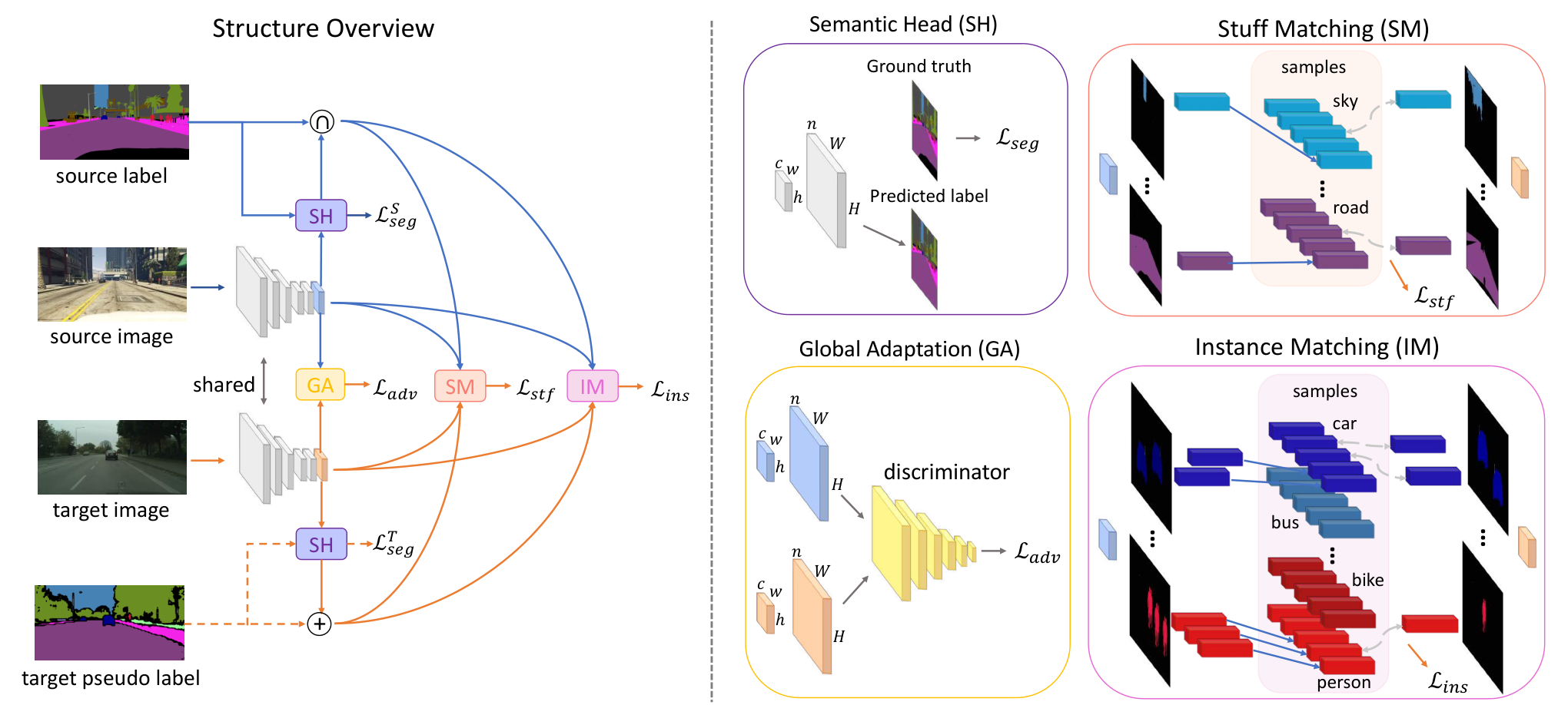
The key idea of our method is that the past experience leading to good outcomes should also help the current training process. Specifically to our task, the past experience should help both the feature-level transferring and the label-level transferring from the source domain to the target domain. First, we raise a stuff and instance matching (SIM) framework to reduce the intra-class domain shift problem. Second, we propose a self-supervised learning framework combined with our proposed SIM structure to enable the label-level transferring, which further boosts the performance. The overall framework is shown in figure 3.

4.1 Stuff and instance matching (SIM)

First, we discuss the matching process for the background classes such as road, sidewalk, sky and etc.. These classes usually cover a large area of the image and lack appearance variation, so we only extract the image-level stuff feature representation for them. For each source domain image, we access the correctly classified label map by selecting the predicted labels matched with the ground truth labels in Eqn (4).

\begin{split}L_{P_{i}}^{s}&=\argmax_{k\in N}(C(f_{i}^{s})^{(k)})\\ L_{C_{i}}^{s}&=L_{G_{i}}^{s}\cap L_{P_{i}}^{s}\end{split}\vskip-5.69054pt

(4)

where $L_{C_{i}}^{s}$ is the correctly classified label map, $L_{G_{i}}^{s}$ is the ground truth label map, $L_{P_{i}}^{s}$ is the predicted label map, and $i\in\{1..|X^{S}|\}$ . We average the features belonging to the same background semantic class across the width and height of the image as the stuff representation for each background class in Eqn (5).

\begin{split}\mathcal{A}^{b}(L,f)&=\frac{\sum_{h,w}\delta({L}^{(h,w)}-b){f}^{(h,w)}}{\max(\epsilon,\sum_{h,w}\delta({L}^{(h,w)}-b))}\\ S^{b}_{j}&=\mathcal{A}^{b}(L_{C_{i}}^{s},f_{i}^{s})\;\;\textbf{where}\;j=i\,\textrm{mod}\,w,\\ &\quad\quad\quad\quad\quad\quad\quad\textbf{if}\;\mathcal{A}^{b}(L_{C_{i}}^{s},f_{i}^{s})\neq 0\end{split}\vskip-5.69054pt

(5)

where $S^{b}_{j}$ is the $j$ ’th source domain semantic feature sample of class $b$ , $b\in B$ (background classes), $i\in\{1..|X^{S}|\}$ , $w$ is the number of feature samples to be stored for each class, $\delta$ is the Dirac delta function and $\epsilon$ is a regularizing term. For each target domain image, we minimize the distance of the stuff representation of each background class with the closest intra-class source stuff feature representation. Because the ground truth of the target domain image is not provided, we use the predicted label map to generate the stuff feature representation for each background class. We adapt the stuff feature representation of the background classes by minimizing the loss function defined in Eqn (6) when the model is trained on the target domain.

\mathfrak{L}_{stf}=\sum_{i}\sum_{b}\min_{j}\mathinner{\!\left\lVert\mathcal{A}^{b}(L_{P_{i}}^{t},f_{i}^{t})-S^{b}_{j}\right\rVert}^{1}_{1}\vskip-5.69054pt

(6)

where $i\in\{1..|X^{T}|\}$ , and $b\in L_{P_{i}}^{t}\cap B$ .

Second, we discuss the instance matching process for the foreground classes such as cars, persons and etc.. Because the ground truth does not provide the instance level annotations, we generate the foreground instance mask by finding the disconnected regions for each foreground class in the label map $L$ . This coarsely segment the intra-class semantic regions into multiple instances, and thus various instance-level feature representations of one image can be generated accordingly in Eqn (7).

\begin{split}R_{k}=\{r_{k_{1}},r_{k_{2}},...,r_{k_{m}}\}=\mathcal{T}(L,k)\\ \mathcal{I}(r,f)=\frac{\sum_{h,w}r^{(h,w)}f^{(h,w)}}{\max({\epsilon,\sum_{h,w}r^{(h,w)}})}\end{split}\vskip-5.69054pt

(7)

where $r_{k_{i}}$ is the $i$ ’th ( $i\in\{1,..,m\}$ ) binary mask of the connected region belonging to class $k$ , $k\in K$ (foreground classes), $\mathcal{T}$ is the operation to find the disconnected regions of class $k$ from the label mask $L$ , and $\mathcal{I}$ is the operation to generate the instance-level feature representation. The source domain instance feature samples can be generated in algorithm 1. Therefore, the target domain instance features can be pulled closer to the closest intra-class source domain instance feature sample by minimizing the loss function in Eqn (8).

\mathfrak{L}_{ins}=\sum_{i}\sum_{k\in K}\frac{1}{\mathinner{\!\left\lvert R^{t}_{k}\right\rvert}}\sum_{r^{t}\in R^{t}_{k}}\min_{j}\mathinner{\!\left\lVert\mathcal{I}(r^{t},f_{i}^{t})-S^{k}_{j}\right\rVert}^{1}_{1}\vskip-5.69054pt

(8)

where $i\in\{1..|X^{T}|\}$ , and $R_{k}^{t}=\mathcal{T}(L_{P_{i}}^{t},k)$ .

Result:

S^{k}

z=10

; # maximum class instances in an image

c_{k}=0,\forall k\in K

; # instance feature counter
for $x_{i}^{s}\in X^{S}$ do

for $k\in K$ do

R_{k}^{s}=\mathcal{T}(L_{C_{i}}^{s},k)

if $R_{k}^{s}\neq\emptyset$ then

R_{sort}

= sort

R_{k}^{s}

by area in descent order
for $l\in\{1..\min(z,\mathinner{\!\left\lvert R_{sort}\right\rvert})\}$ do

j=c_{k}\mod z*w

c_{k}=c_{k}+1

S^{k}_{j}=\mathcal{I}(R_{sort}[l],f_{i}^{s})

end for

end if

end for

Algorithm 1 Instance-level source feature samples

4.2 Self-supervised learning with SIM

Because the model is only trained on the source domain with the ground truth annotations, the features and the softmax output are thus generated to optimize the source domain segmentation loss function but ignore the target domain segmentation supervision. However, the distribution of the ground truth labels from both domains also have a discrepancy, and this negatively impacts the model’s performance on the target domain. Therefore, we propose a self supervised learning framework combined with our feature matching methods to alleviate this problem.

We first follow the framework described in sections 3 and 4.1 to train a model with the source domain images $X^{S}$ and ground truth annotations $Y^{S}$ along with the target domain images $X^{T}$ . Then we use the trained model to give pseudo-labels to the pixels with high confidence of the predicted labels in the training set images $X^{T}$ shown in Eqn (9).

\hat{y}^{t}_{i}=\argmax_{k\in N}\mathbbm{1}_{[\mathcal{S}(C(f_{i}^{t}))^{(k)}>y_{t}^{k}]}(C(f_{i}^{t})^{(k)})\vskip-5.69054pt

(9)

where $\mathbbm{1}$ is a function which returns the input if the condition is true or a don’t care symbol if not, and $y_{t}^{k}$ is the confidence threshold for class $k$ . Then, we add the semantic segmentation loss on the target domain images in Eqn (10) along with other losses to retrain our model.

\mathfrak{L}_{seg}^{T}(f^{t})=-\sum_{i,h,w}\sum_{k\in N}\hat{y}^{(h,w)}_{i}\log(\mathcal{S}(C(f^{t}_{i})^{(h,w)})^{(k)})\vskip-5.69054pt

(10)

With the pseudo labels supervising the model to generate features corresponding to specific classes, these features should generically be adapted to be closer to the corresponding intra-class source domain features. The $L_{P_{i}}^{t}$ is thereby augmented by Eqn (11) for the stuff feature adaptation loss defined in Eqn (6) and the instance feature adaptation loss defined in Eqn (8):

\mathbbm{1}_{L_{P_{i}}^{t}\neq\hat{y}_{i}^{t}}(L_{P_{i}}^{t})=\mathbbm{1}_{L_{P_{i}}^{t}\neq\hat{y}_{i}^{t}}(\hat{y}_{i}^{t}).\vskip-5.69054pt

(11)

$\mathbbm{1}$ selects the positions in the input satisfying the condition.

4.3 Training procedure

We follow a two-step training procedure to improve the performance of the generator $G$ on semantic segmentation task on the target domain dataset. First, we train our model without the self-supervised learning module, and optimize the target function in Eqn (12) with $G$ and $D$ in an adversarial training strategy:

\begin{split}\min_{G,D}\mathfrak{L}_{step1}=&\min_{G}(\lambda_{seg}\mathfrak{L}_{seg}^{S}+\lambda_{adv}\mathfrak{L}_{adv}+\\ &\lambda_{ci}(\mathfrak{L}_{stf}+\mathfrak{L}_{ins}))+\min_{D}\lambda_{D}\mathfrak{L}_{D},\end{split}\vskip-5.69054pt

(12)

where $\lambda$ ’s are the weight parameters for the losses. Second, after giving the pseudo labels to the target domain training dataset with the model trained in the first step, we reinitialize and repeat the training process to optimize the loss function in Eqn (13).

\begin{split}\min_{G,D}\mathfrak{L}_{step2}=&\min_{G}(\lambda_{seg}(\mathfrak{L}_{seg}^{S}+\mathfrak{L}_{seg}^{T})+\lambda_{adv}\mathfrak{L}_{adv}+\\ &\lambda_{ci}(\tilde{\mathfrak{L}}_{stf}+\tilde{\mathfrak{L}}_{ins}))+\min_{D}\lambda_{D}\mathfrak{L}_{D},\end{split}\vskip-5.69054pt

(13)

where $\tilde{\mathfrak{L}}_{stf}$ and $\tilde{\mathfrak{L}}_{ins}$ are augmented with predicted $\hat{y}^{t}_{i}$ s according to Eqn (11).

Table 1: Comparison to the state-of-the-art results of adapting GTA5 to Cityscapes.

GTA5 $\rightarrow$ Cityscapes
Method	road	sidewalk	building	wall	fence	pole	light	sign	vegetation	terrain	sky	person	rider	car	truck	bus	train	motorbike	bike	mIoU
Wu et al.wu	85.0	30.8	81.3	25.8	21.2	22.2	25.4	26.6	83.4	36.7	76.2	58.9	24.9	80.7	29.5	42.9	2.5	26.9	11.6	41.7
Tsai et al.outputspace	86.5	36.0	79.9	23.4	23.3	23.9	35.2	14.8	83.4	33.3	75.6	58.5	27.6	73.7	32.5	35.4	3.9	30.1	28.1	42.4
Saleh et al.saleh	79.8	29.3	77.8	24.2	21.6	6.9	23.5	44.2	80.5	38.0	76.2	52.7	22.2	83.0	32.3	41.3	27.0	19.3	27.7	42.5
Luo et al. Luo_2019_CVPR	88.5	35.4	79.5	26.3	24.3	28.5	32.5	18.3	81.2	40.0	76.5	58.1	25.8	82.6	30.3	34.4	3.4	21.6	21.5	42.6
Hong et al.hong	89.2	49.0	70.7	13.5	10.9	38.5	29.4	33.7	77.9	37.6	65.8	75.1	32.4	77.8	39.2	45.2

Differential Treatment for Stuff and Things: A Simple Unsupervised Domain Adaptation Method for Semantic Segmentation