PolyFit: Polynomial-based Indexing Approach for Fast Approximate Range Aggregate QueriesConference: 24th International Conference on Extending Database Technology (EDBT); Nicosia; CyprusNote: This work was supported by grant GRF 152050/19E from the Hong Kong RGC.

Zhe Li

{}^{\text{1}}

, Tsz Nam Chan

{}^{\text{2}}

, Man Lung Yiu

{}^{\text{1}}

, Christian S. Jensen

{}^{\text{3}}

Affiliation: Hong Kong Polytechnic University

{}^{\text{1}}

, Hong Kong Baptist University

{}^{\text{2}}

, Aalborg University

{}^{\text{3}}

richie.li@connect.polyu.hk, edisonchan@comp.hkbu.edu.hk, csmlyiu@comp.polyu.edu.hk, csj@cs.aau.dk

2021

Abstract.

Range aggregate queries find frequent application in data analytics. In many use cases, approximate results are preferred over accurate results if they can be computed rapidly and satisfy approximation guarantees. Inspired by a recent indexing approach, we provide means of representing a discrete point dataset by continuous functions that can then serve as compact index structures. More specifically, we develop a polynomial-based indexing approach, called PolyFit, for processing approximate range aggregate queries. PolyFit is capable of supporting multiple types of range aggregate queries, including COUNT, SUM, MIN and MAX aggregates, with guaranteed absolute and relative error bounds. Experimental results show that PolyFit is faster and more accurate and compact than existing learned index structures.

1. Introduction

A range aggregate query (ho1997range) retrieves records in a dataset that belong to a given key range and then applies an aggregate function (e.g., SUM, COUNT, MIN, MAX) to an attribute of those records. Range aggregate queries are used in OLAP (vitter1999approximate; ho1997range) and data analytics applications, e.g., for outlier detection (XGGKS15; ES13), data visualization (AMSAKS15), and tweet analysis (AMODSR11). For example, network intrusion detection systems (XGGKS15) utilize range COUNT queries to monitor a network for anomalous activities. Furthermore, applications with huge numbers of users are expected to receive queries frequently. For instance, Foursquare, with more than 50 million monthly active users (Foursquareusers), helps users find the number of specific POIs (e.g., restaurants) within given regions (FoursquareAPI). In many application scenarios, users accept approximate results provided that (i) they can be computed quickly and (ii) they are sufficiently accurate (e.g., within 5% error). We target such applications and focus on error-bounded evaluation of range aggregate queries.

A recent indexing approach represents the values of attributes in a dataset by continuous functions, which then serve to enable compact index structures (kraska2018case; fiting2019). When compared to traditional index structures, this approach is able to yield a smaller index size and faster response time. The existing studies (kraska2018case; fiting2019) focus on computing exact results for point and range queries on 1-dimensional data. In contrast, we conduct a comprehensive study of approximate range aggregate queries, supporting many aggregate functions and multi-dimensional data.

The idea that underlies our proposal for using functions to answer approximate range aggregate queries may be explained as follows. Consider a stock market index (e.g., the Hong Kong Hang Seng Index) at different times as a dataset $\mathcal{D}$ consisting of records of the form (index value, timestamp), where the former is our measure and the latter is our key that is used for specifying query ranges—see Figure 1(a). A user can find the average stock market index value in a specified time range $[l_{q},u_{q}]$ by issuing a range SUM query (and divide by $u_{q}-l_{q}+1$ ). We propose to construct the cumulative function of $\mathcal{D}$ as shown in Figure 1(b). If we can approximate this function well by a polynomial function $\mathbb{P}(x)$ then the range SUM query can be approximated as $\mathbb{P}(u_{q})-\mathbb{P}(l_{q})$ , which takes $O(1)$ time. As another example, the user may wish to find the maximum stock market index in a specified time range. The timestamped index values in $\mathcal{D}$ can be modeled by the continuous function shown in Figure 1(c). Again, if we can approximate this function well using a polynomial function $\mathbb{P}(x)$ then the range MAX query can be answered quickly using mathematical tools, e.g., by applying differentiation to identify maxima in $\mathbb{P}(x)$ .

Regarding the two-dimensional case, consider the dataset of tweets’ locations as shown in Figure 9(a) in Section 6, where each data point has a longitude (as key 1) and a latitude (as key 2). Suppose that the user wishes to count the number of tweets in a geographical region. Our idea is to derive the cumulative count function shown in Figure 9(b), and then approximate this function with a polynomial function $\mathbb{P}(x_{1},x_{2})$ (of two variables). This enables us to answer a two-dimensional range COUNT query in $O(1)$ time.

(a) timestamped index values

(b) function for range SUM queries

Figure 1. Stock market index values, 1-dimensional keys: discrete data points vs. continuous function

Another difference between our work and existing studies (kraska2018case; fiting2019) is the types of functions used for approximation. Our proposal uses piecewise polynomial functions, rather than piecewise linear functions (kraska2018case; fiting2019). As we will show in Section 4, using polynomial functions yields lower fitting errors than using linear functions. Thus, our proposal leads to smaller index sizes and faster queries.

The key technical challenges are as follows. (1) How to find polynomial functions with low approximation error efficiently? (2) How to answer range aggregate queries with error guarantees? (3) How to support common aggregate functions (e.g., COUNT, SUM, MIN, MAX) and multi-dimensional data?

To tackle these challenges, we develop a polynomial-based indexing approach (PolyFit) for processing approximate range aggregate queries. Our contributions are summarized as follows.

•

To the best of our knowledge, this is the first study that utilizes polynomial functions to learn indexes that support approximate range aggregate queries.
•

PolyFit supports multiple types of range aggregate queries, including COUNT, SUM, MIN and MAX with guaranteed deterministic absolute and relative error bounds.
•

Experiment results show that PolyFit achieves significant speedups, compared with the closest related works (fiting2019; kraska2018case), and traditional exact/approximate methods. For instance, for the OpenStreetMap dataset with 100M records, our index occupies only 4 MBytes and offers 5 $\mu s$ query response time (per 2-dimensional range COUNT query).

The rest of the paper is organized as follows. We first review the related work in Section 2. Next, we introduce preliminaries in Section 3. Then, we present our index construction techniques in Section 4 and cover how to answer approximate range aggregate queries in Section 5. Next, we extend our proposal to datasets with two keys in Section 6. Lastly, we present experiments in Section 7 and conclude in Section 8.

2. Related Work

Range aggregate queries are used frequently in analytics applications and constitute important functionality in OLAP and data warehousing (momjian2001postgresql; delaney2000inside; bartholomew2014mariadb; condie2010online; armbrust2015spark; jensen2018modelardb; vitter1999approximate; ho1997range). Exact solutions are based on prefix-sum arrays (ho1997range) or aggregate R-trees (DPJY01). Due to the need for real-time performance in some applications (e.g., $\mu s$ -level response time (XGGKS15)), many proposals exist that aim to improve the efficiency of range aggregate queries. These proposals can be classified as being either data-driven or query-driven. In addition, we also review some other studies, including learned indexes, and time series databases, which are also related to this work.

Data-driven proposals build statistical models of a dataset for estimating query selectivity or the results of range aggregate queries. These models employ multi-dimensional histograms (lynch1988selectivity; muralikrishna1988equi; ilyas2004cords; to2013entropy), data sampling (lipton1990practical; haas1994relative; riondato2011vc; BlinkDB13; VerdictDB18; han2019iterative), or kernel density estimation (gunopulos2000approximating; gunopulos2005selectivity; heimel2015self). Although such proposals that compute approximate results are much faster than exact solutions, e.g., achieving ms ( $10^{-3}$ ) level response time (park2018quicksel), they still do not offer real-time performance (e.g., $\mu s$ level (XGGKS15)). Furthermore, these proposals do not offer theoretical approximation error guarantees.

The query-driven approaches utilize query workloads to build statistical models of datasets. Typical methods include error-feedback histograms (aboulnaga1999self; lim2003sash; anagnostopoulos2015learning), max-entropy histograms (markl2007consistent; Re:2012:UCE:2109196.2109202), and learning-based models (QP19; PeterAggregate2019). In addition, Park et al. (park2018quicksel) explore the approach of using mixture probabilistic models. These methods assume that new queries follow historical query workload distributions. However, as one study (BJCGF04) observes, this assumption may not always hold in practice. Further, even when this assumption is valid, the number of queries that are similar to those used for training may be much smaller if the queries follow a power law distribution (yu2018sundial), which can cause poor accuracy and may render it impossible to obtain useful approximation error guarantees for range aggregate queries.

Recently, learning-based methods have been used to construct more compact and effective index structure, that hold potential to accelerate database operations. Kraska et al. (kraska2018case) propose the RMI index, which incorporates different machine learning models, e.g., linear regression and deep-learning, to improve the efficiency of range queries. Galakatos et al. (fiting2019) develop the FITing-tree, which is a segment-tree-like structure (SegmentTreeBook; AXNS17) that can significantly improve the efficiency of exact point queries. Ferragina et al. (PG20) further support efficient update operations for range queries. Wang et al. (WangFX019) extend this learning-based approach to the spatial domain with their learned Z-order model that aims to support fast spatial indexing. However, there are two main differences between these proposals and our proposal. First, they either support range queries (kraska2018case; WangFX019; PG20) or point queries (fiting2019), but not range aggregate queries. Second, we are the first to exploit polynomial functions to build index structures for approximate range aggregate queries.

In the time series database community, some research studies utilize mathematical models to approximate time series data. Representative approaches include piecewise linear approximation (Plato20; Online2001; PLAKDD98; FastSimSearchKeogh97; HazemSwingSlide2009), discrete wavelet transform (WavletICDE02; WavletICDE99), discrete Fourier transform (DFTSIGMOD94; DFTICDE99), and their combinations (EamonnTKDE08; jensen2018modelardb). However, these studies focus on either time series similarity search (e.g., range or nearest neighbor queries) or time series compression and they are not designed to answer the range aggregate queries we target. Some of these studies also utilize piecewise linear approximation (Plato20; Online2001; HazemSwingSlide2009; FastSimSearchKeogh97) to approximate time-series, which we also do. In contrast, we achieve better performance by utilizing nonlinear (polynomial) functions to approximate curves, which can reduce the number of segments dramatically. Furthermore, we can also support the segmentation of surfaces (e.g., Figure 9(b)), rather than only 1-D curves.

3. Preliminaries

First, we define range aggregate queries and their approximate versions in Section 3.1. Then, we discuss the baselines for answering exact range aggregate queries in Section 3.2. Table 1 summarizes frequently used symbols in this paper.

Table 1. Symbols

Symbol	Description
$\mathcal{D}$	dataset
$n$	number of records in $\mathcal{D}$
$R_{count}$	range `COUNT` query
$R_{sum}$	range `SUM` query
$R_{min}$	range `MIN` query
$R_{max}$	range `MAX` query
$CF_{sum}$	cumulative function for range `SUM` query
$DF_{max}$	key-measure function for range `MAX` query
$\mathbb{P}(k)$	polynomial function
$I$	interval
$deg$	degree of polynomial function

3.1. Problem Definition

We focus on the setting that a range aggregate query specifies a $key$ attribute (for range selection) and a $measure$ attribute for aggregation. We shall consider the setting of two keys in Section 6. As such, the dataset $\mathcal{D}$ is a set of $(key,measure)$ records, i.e., $\mathcal{D}=\{(k_{1},m_{1}),(k_{2},m_{2}),...,(k_{n},m_{n})\}$ . For ease of discussion, we assume that key values are distinct and measure values are numerical. We leave the discussion of repeated keys and negative measure values in Appendices A.3 and A.4 (ZTMC20_arxiv). Then we define a range aggregate query as follows.

Definition 3.1.

Let $\mathcal{G}$ be an aggregate function (e.g., COUNT, SUM, MIN, MAX) on a measure attribute. Given a dataset $\mathcal{D}$ and a key range $[l_{q},u_{q}]$ , we define $V$ as the following multi-set

V=\{m\mid(k,m)\in\mathcal{D}\wedge l_{q}\leq k\leq u_{q}\}

and then define the result of the range aggregate query as

(1)

R_{\mathcal{G}}(\mathcal{D},[l_{q},u_{q}])=\mathcal{G}(V).

We aim to develop efficient methods for obtaining an approximate result of $R_{\mathcal{G}}(\mathcal{D},[l_{q},u_{q}])$ with two types of error guarantees (MP02; MP04), namely the absolute error guarantee (cf. Problem 1) and the relative error guarantee (cf. Problem 2).

Problem 1 ( $Q_{abs}$ ).

Given an absolute error $\varepsilon_{abs}$ and a range aggregate query, we ask for an approximate result $A_{abs}$ such that:

(2)

|A_{abs}-R_{\mathcal{G}}(\mathcal{D},[l_{q},u_{q}])|\leq\varepsilon_{abs}

Problem 2 ( $Q_{rel}$ ).

Given a relative error $\varepsilon_{rel}$ and a range aggregate query, we ask for an approximate result $A_{rel}$ such that:

(3)

\left|\frac{A_{rel}-R_{\mathcal{G}}(\mathcal{D},[l_{q},u_{q}])}{R_{\mathcal{G}}(\mathcal{D},[l_{q},u_{q}])}\right|\leq\varepsilon_{rel}

3.2. Baselines: Exact Methods

We proceed to discuss exact methods for answering range SUM queries and range MAX queries. These methods can be easily extended to support COUNT and MIN, respectively.

3.2.1. Exact method for range SUM queries

First, we define the key cumulative function as $CF_{sum}(k)$ :

(4)

CF_{sum}(k)=R_{sum}(\mathcal{D},[-\infty,k]).

The additive property of $CF_{sum}$ enables us to compute the exact result of the range SUM query as:

(5)

R_{sum}(\mathcal{D},[l_{q},u_{q}])=CF_{sum}(u_{q})-CF_{sum}(l_{q}).

Then, we discuss how to obtain the terms $CF_{sum}(l_{q})$ and $CF_{sum}(u_{q})$ efficiently. Although $CF_{sum}$ is a continuous function, it can be expressed by a discrete data structure in finite space. Specifically, we presort dataset $\mathcal{D}$ in ascending key order and then follow this order to construct a key-cumulative array of entries $(k,CF_{sum}(k))$ . At query time, the terms $CF_{sum}(l_{q})$ and $CF_{sum}(u_{q})$ are obtained by performing binary search on the above key-cumulative array. This step takes $O(\log n)$ time.

As a remark, this key-cumulative array is similar to the prefix-sum array (ho1997range). The difference is that our array allows floating-point search keys, while the prefix-sum array does not.

3.2.2. Exact method for range MAX queries

First, we define the key-measure function $DF_{max}(k)$ in Equation 6 to capture the data distribution in the dataset $\mathcal{D}$ . In the definition, we assume that each pair $(k_{i},m_{i})$ in $\mathcal{D}$ is arranged in ascending order by the key.

(6)

\displaystyle DF_{max}(k)=\begin{cases}m_{1}&\mbox{ if }k_{1}\leq k<k_{2}\\ \vdots&\mbox{ }\vdots\\ m_{i}&\mbox{ if }k_{i}\leq k<k_{i+1}\\ \vdots&\mbox{ }\vdots\\ m_{n}&\mbox{ if }k=k_{n}\\ -\infty&\mbox{ otherwise}\\ \end{cases}

Figure 2(a) exemplifies the function $DF_{max}(k)$ .

An aggregate max-tree (DPJY01) (cf. Figure 2(b)) can be built to answer range MAX queries. In this tree, each internal node stores two entries, where each entry stores an interval and the maximum measure within that interval (e.g., $(I_{1},m_{6})$ and $(I_{2},m_{7})$ are two entries of the root node $N_{root}$ ). We then explain how to process the query $R_{max}(\mathcal{D},[l_{q},u_{q}])$ , whose query range is indicated by the red line in Figure 2(a). In Figure 2(b), we start from the root of the tree. If the interval of an entry intersects with the query range (e.g., $I_{1}$ and $I_{2}$ in Figure 2(a)), we visit its child nodes (e.g., $N_{1}$ and $N_{2}$ ). When the interval of an entry (e.g., $I_{4}$ and $I_{5}$ in Figure 2a) is covered by the query range, we directly use its stored aggregate value without visiting its child nodes (e.g., yellow nodes in Figure 2b). During the traversal, we keep track of the maximum measure seen so far. This procedure takes $O(\log n)$ time as we check at most two branches per level.

Figure 2. Aggregate MAX tree

4. Index Construction

Traditional index structures (e.g., B-tree (TCRC01)) need to store $n$ keys, where $n$ is the cardinality of the dataset $\mathcal{D}$ . Thus, the index size grows linearly with the data size. To reduce the index size dramatically, we plan to index a limited number of functions (instead of $n$ keys).

As a case study, we compare existing fitting functions (kraska2018case; fiting2019) with our fitting function (polynomial) on a real dataset (the Hong Kong 40 Index in 2018 (hk40index)) in Figure 3. The exact key-measure function $DF_{max}(k)$ exhibits a complex shape. Observe that linear functions, e.g., linear regression $LR(k)$ (kraska2018case) and linear segment $FIT(k)$ (fiting2019), cannot accurately approximate the exact function. In this paper, we adopt the polynomial function $\mathbb{P}(k)$ , which captures the nonlinear property¹¹ 1 As a remark, other types of nonlinear functions (e.g., logarithmic and trigonometric functions) require higher computation cost than polynomial functions. Thus, we leave other types of nonlinear functions as future work. and achieves a better approximation of $DF_{\max}(k)$ . In this example, $\mathbb{P}(k)$ is a degree-4 polynomial function (blue dotted line).

Figure 3. Curve fitting of the HKG 40 Index in 2018 (hk40index)

Figure 4. Indexing framework for PolyFit, each leaf entry stores a polynomial function

We introduce our indexing framework in Figure 4. First, we convert the dataset into the following exact function $F(k)$ based on the aggregate function $\mathcal{G}$ and the functions in Section 3.2.

(7)

\displaystyle F(k)=\begin{cases}CF_{sum}(k)&\text{if }\mathcal{G}=\texttt{SUM}\\ DF_{max}(k)&\text{if }\mathcal{G}=\texttt{MAX}\end{cases}

We plan to compute an error-bounded approximation of $F(k)$ by using a sequence of polynomial functions. In Section 4.1, we examine how to find the best polynomial fitting of $F(k)$ in a given key interval $I$ . Then, in Section 4.2, we propose a segmentation method for $F(k)$ in order to minimize the index size subject to a given deviation threshold. Finally, in Section 4.3, we discuss how to build an index for a sequence of polynomial functions.

4.1. Polynomial Fitting in a Key Interval

We discuss how to find the best fitting polynomial function of $F(k)$ in a given key interval $I$ . First, we express a polynomial function $\mathbb{P}(k)$ as follows:

(8)

\mathbb{P}(k)=\sum_{j=0}^{deg}a_{j}k^{j},

where $deg$ is the degree and each $a_{j}$ is a coefficient. Note that the choice of $deg$ entails tradeoffs between the fitting error and the online query evaluation cost. We discuss the choice of $deg$ in Section 5.3.

We formulate the following optimization problem in order to minimize the fitting error between $\mathbb{P}(k)$ and $F(k)$ .

Definition 4.1.

Let $F(k)$ be the exact function and $I$ be a given key interval. Let $k_{1},k_{2},\cdots,k_{\ell}$ be the keys of $\mathcal{D}$ in interval $I$ . We aim to find polynomial coefficients, $a_{0},a_{1},\cdots,a_{deg}$ that minimize the following error:

(9)

E(I)=\min_{a_{0},a_{1},...,a_{deg}\in\mathbb{R}}\;\max_{1\leq i\leq\ell}|F(k_{i})-\mathbb{P}(k_{i})|

This is equivalent to the following linear programming problem, where the coefficients $a_{0},a_{1},\cdots,a_{deg}$ and $t$ are variables.

(10)

\begin{cases}&\textsc{minimize}\quad t\\ &\textsc{subject \> to:}\\ &-t\leq F(k_{1})-(a_{deg}k_{1}^{deg}+...+a_{2}k_{1}^{2}+a_{1}k_{1}+a_{0})\leq t\\ &-t\leq F(k_{2})-(a_{deg}k_{2}^{deg}+...+a_{2}k_{2}^{2}+a_{1}k_{2}+a_{0})\leq t\\ &...\\ &-t\leq F(k_{\ell})-(a_{deg}k_{\ell}^{deg}+...+a_{2}k_{\ell}^{2}+a_{1}k_{\ell}+a_{0})\leq t\\ &\forall a_{i}\in\mathbb{R}\\ \end{cases}

It takes $O(\ell^{2.5})$ time to solve the above linear programming problem (Equation 10) (lee2015efficient). In our experimental study, we adopt the IBM CPLEX linear programming library as the LP Solver, which is believed to be the most reliable and efficient among other implementations (LPSolverComparison). We discuss some subtle issues like precision limitations in Section 5.3.

4.2. Minimal Index Size with Bounded Error

To support approximate query evaluation (in Section 5), we require that the fitting polynomial functions should satisfy a given error constraint. However, a single polynomial function is unlikely to fit accurately for the entire key domain. Thus, we propose to partition the key domain into intervals $I_{1},I_{2},\cdots,I_{h}$ so that each interval $I_{i}$ satisfies the following requirement:

E(I)\leq\delta,

where $\delta$ is a given deviation threshold. For instance, in Figure 5, the key domain is partitioned into two intervals $I_{1}$ and $I_{2}$ so that the best fitting polynomial function in each interval satisfies the error requirement.

Figure 5. Fitting

F(k)

with multiple polynomial functions, subject to the deviation threshold

\delta

To achieve a small index size, we aim to minimize the number of intervals (i.e., $h$ in Figure 4). An existing dynamic programming (DP) approach (leenaerts2013piecewise), though designed for piecewise linear functions, can be adapted to solve our partitioning problem of $F(k)$ . However, this method takes $O(n^{2}\times\ell_{max}^{2.5})$ time²² 2 Recall that the state-of-the-art linear programming solver (lee2015efficient) takes $O(\ell_{max}^{2.5})$ time for each curve-fitting problem (cf. Equation 10)., where $\ell_{max}$ is the maximum number of keys covered by any interval. Obviously, this method does not scale well with the data size $n$ .

In Section 4.2.1, we present a more efficient method, called greedy segmentation (GS), to segment the exact function $F(k)$ . As we show later, the time complexity of GS is $O(n\times\ell_{max}^{2.5})$ , which scales well with the data size $n$ . Then, in Section 4.2.2, we show that GS is guaranteed to return the optimal solution.

4.2.1. Greedy Segmentation (GS) Method

We present the pseudo-code of the Greedy Segmentation (GS) method in Algorithm 1. It examines the key domain from left to right (line 2). In each iteration, it expands the interval $I$ by including the next key (line 3), calls an LP solver on the interval $I$ to obtain a fitting function $\mathbb{P}_{now}$ (line 4), and tests whether it fulfills the error requirement. When this test fails (i.e., $E(I)>\delta$ ), we conclude that the previous interval is a maximal interval and thus insert its corresponding fitting function $\mathbb{P}_{prev}$ into the result. The above procedure is repeated until all keys are covered.

Algorithm 1 Greedy Segmentation (GS)

1: Input: function

F(k)

, degree

deg

, deviation threshold

\delta

2: Output: sequence of polynomial functions

\text{Seq}_{\mathbb{P}}

\text{Seq}_{\mathbb{P}}\leftarrow\emptyset

;

l\leftarrow 1

;

\mathbb{P}_{prev}\leftarrow null

4: for

u\leftarrow 2

n

I\leftarrow[k_{l},k_{u}]

\triangleright

the interval for polynomial function

\mathbb{P}

\mathbb{P}_{now}\leftarrow

call LP solver on

I

\triangleright

Equation 10

7: if

E(I)>\delta

u=n

then

\triangleright

Equation 9

8: insert

\mathbb{P}_{prev}

into

\text{Seq}_{\mathbb{P}}

l\leftarrow u

10:

\mathbb{P}_{prev}\leftarrow\mathbb{P}_{now}

11: return

\text{Seq}_{\mathbb{P}}

The time complexity of GS is $O(n\ell_{max}^{2.5})$ because it invokes $O(n)$ calls to the LP solver, where each call takes $O(\ell_{max}^{2.5})$ time (lee2015efficient). We further accelerate GS by applying an existing exponential search technique (JA76), which can reduce the number of LP calls per interval by $\frac{\ell}{\log\ell}$ times. With this technique, GS takes only 70 seconds (cf. Section 7.2.2) to complete for a real dataset with 1 million data points. This is acceptable for many data analytics tasks (with static datasets) in OLAP. In our experiments, we find that $\ell_{max}$ usually ranges between hundreds and thousands, thus the term $O(\ell_{max}^{2.5})$ is acceptable in practice. In Appendix (ZTMC20_arxiv), we discuss how to utilize parallel computation to further improve the construction time.

4.2.2. GS is Optimal

We first prove the following property (Lemma 4.2) of our curve fitting problem (cf. Definition 4.1).

Lemma 4.2.

Let $I_{l}$ and $I_{u}$ be two intervals, which contain two sets of keys $S_{l}$ and $S_{u}$ , respectively. If $S_{l}\subseteq S_{u}$ , then $E(I_{l})\leq E(I_{u})$ .

Proof.

Recall that the value of $E(I)$ (cf. Equation 9) is equal to the minimum value of the optimization problem (Equation 10). Since $S_{l}$ is a subset of $S_{u}$ , the set of constraints for solving $E(I_{l})$ is also the subset of constraints for solving $E(I_{u})$ . Thus, for the minimization problem in Equation 10, the possible solution space for $S_{l}$ is a superset of the possible solution space for $S_{u}$ . Therefore, we conclude that $E(I_{l})\leq E(I_{u})$ . ∎

Based on Lemma 4.2, we then show that GS produces the fewest polynomial functions (cf. Theorem 4.3), i.e., the optimal solution.

Theorem 4.3.

GS always produces the optimal number of functions (with respect to the given parameters $deg$ and $\delta$ ).

Proof.

We denote the minimum key and the maximum key of an interval $I$ by $I.\min$ and $I.\max$ , respectively.

Let $\mathcal{I}_{\text{OPT}}^{*}=(I_{\text{OPT}}^{(1)},I_{\text{OPT}}^{(2)},\cdots)$ and $\mathcal{I}_{\text{GS}}^{*}=(I_{\text{GS}}^{(1)},I_{\text{GS}}^{(2)},\cdots)$ be two ascending sequences of intervals for the optimal solution and our GS method, respectively (i.e., $I^{(i)}.\max<I^{(i+1)}.\min$ for $i=1,2,...,n-1$ ). Every interval $I$ in $\mathcal{I}_{\text{OPT}}^{*}$ and $\mathcal{I}_{\text{GS}}^{*}$ must satisfy $E(I)\leq\delta$ . We now prove the theorem by mathematical induction.

In the base step, we consider the first interval in each sequence. Since both GS and OPT must cover the key domain, we have:

I_{\text{GS}}^{(1)}.\min=I_{\text{OPT}}^{(1)}.\min

According to GS, the first interval $I_{\text{GS}}^{(1)}$ is maximal, because a longer interval would violate the deviation threshold $\delta$ . Thus, we have:

(11)

I_{\text{GS}}^{(1)}.\max\geq I_{\text{OPT}}^{(1)}.\max

In the inductive step, assume that the first $\ell$ intervals of the two sequences satisfy the following property:

(12)

I_{\text{GS}}^{(\ell)}.\max\geq I_{\text{OPT}}^{(\ell)}.\max

Since $\mathcal{I}_{\text{OPT}}^{*}$ and $\mathcal{I}_{\text{GS}}^{*}$ are ascending sequences of intervals, Equation 12 implies the following:

(13)

I_{\text{GS}}^{(\ell+1)}.\min\geq I_{\text{OPT}}^{(\ell+1)}.\min

Now, we consider two cases for comparing $I_{\text{GS}}^{(\ell+1)}$ and $I_{\text{OPT}}^{(\ell+1)}$ .

Case 1:

I_{\text{GS}}^{(\ell+1)}.\max\geq I_{\text{OPT}}^{(\ell+1)}.\max

In this case, the first $\ell+1$ intervals of GS cover all keys in the first $\ell+1$ intervals of OPT.

Case 2:

(14)

I_{\text{GS}}^{(\ell+1)}.\max<I_{\text{OPT}}^{(\ell+1)}.\max

Consider the interval $I^{\prime}=[I_{\text{GS}}^{(\ell+1)}.\min,I_{\text{OPT}}^{(\ell+1)}.\max]$ . By using Equations 13 and 14, we obtain: $I^{\prime}\subset I_{\text{OPT}}^{(\ell+1)}$ . By Lemma 4.2, we get: $E(I^{\prime})\leq E(I_{\text{OPT}}^{(\ell+1)})$ . Since $E(I_{\text{OPT}}^{(\ell+1)})\leq\delta$ , we get: $E(I^{\prime})\leq\delta$ .

Observe that $I^{\prime}$ has the same minimum key as $I_{\text{GS}}^{(\ell+1)}$ but a larger maximum key than $I_{\text{GS}}^{(\ell+1)}$ . Since $I^{\prime}$ does not pass the error test in GS, we get $E(I^{\prime})>\delta$ . This contradicts the statement $E(I^{\prime})\leq\delta$ .

Therefore, only the first case is true, and we have:

I_{\text{GS}}^{(\ell+1)}.\max\geq I_{\text{OPT}}^{(\ell+1)}.\max

This means GS always covers no fewer keys than OPT with the same number of intervals. Thus, GS produces the optimal number of functions. ∎

4.3. Indexing of polynomial functions

In our experimental study, the number of intervals (for polynomial functions) ranges from 100 to 1000. We adopt existing index structures on these intervals to support fast query evaluation. Specifically, we employ an in-memory index called the STX B-tree (STXBtree) to index intervals. In each internal node entry, we maintain an additional attribute to store the aggregate value of its subtree. In each leaf node entry, we store an interval and its corresponding polynomial model (in the form of coefficients). In summary, this index is similar to the aggregate tree exemplified in Figure 2(b), except that we store polynomial models in leaf nodes.

5. Approximate Query Evaluation

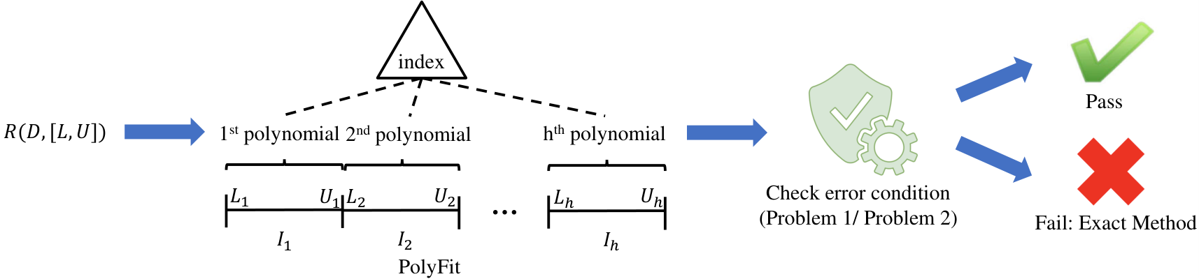
We present our framework for answering approximate range aggregate queries in Figure 6. The first step is to compute an initial approximate result quickly by using our index (PolyFit). Then, we check whether the error condition is satisfied and refine the approximate result if necessary. We discuss how to answer the approximate range SUM query and the approximate range MAX query in Sections 5.1 and 5.2, respectively. Finally, in Section 5.3, we discuss how to tune our index parameters (e.g., $deg,\delta$ ) in order to optimize the query response time.

Refer to caption — Figure 6. Querying framework for PolyFit

5.1. Approximate range SUM Query

Given the query range $[l_{q},u_{q}]$ , we propose to compute the approximate result as:

(15)

\tilde{A}_{sum}=\mathbb{P}_{I_{u}}(u_{q})-\mathbb{P}_{I_{l}}(l_{q}),

where $I_{l}$ and $I_{u}$ denote the intervals of $\mathbb{P}$ that contain the values $l_{q}$ and $u_{q}$ , respectively.

Then, we show the error conditions for $Q_{abs}$ (cf. Problem 1) and $Q_{rel}$ (cf. Problem 2).

Error condition for $Q_{abs}$ Given the absolute error $\varepsilon_{abs}$ , we recommend to use the deviation threshold $\delta=\frac{\varepsilon_{abs}}{2}$ in constructing PolyFit. With this setting, the following lemma offers the absolute error guarantee for the approximate result $\tilde{A}_{sum}$ (in Equation 15).

Lemma 5.1.

If $\delta=\frac{\varepsilon_{abs}}{2}$ , then $\tilde{A}_{sum}$ (in Equation 15) satisfies the absolute error guarantee with respect to $\varepsilon_{abs}$ .

Proof.

Let $I_{l}$ and $I_{u}$ be two intervals (in PolyFit) which contain $l_{q}$ and $u_{q}$ (of the query range $[l_{q},u_{q}]$ ), respectively. Based on the deviation threshold guarantee in Section 4.2.2, we obtain:

|CF_{sum}(l_{q})-\mathbb{P}_{I_{l}}(l_{q})|\leq\delta

|CF_{sum}(u_{q})-\mathbb{P}_{I_{u}}(u_{q})|\leq\delta

By combining them, we have:

CF_{sum}(u_{q})-CF_{sum}(l_{q})-2\delta\leq\tilde{A}_{sum}\leq CF_{sum}(u_{q})-CF_{sum}(l_{q})+2\delta

By using Equation 5, we have:

R_{sum}(\mathcal{D},[l_{q},u_{q}])-2\delta\leq\tilde{A}_{sum}\leq R_{sum}(\mathcal{D},[l_{q},u_{q}])+2\delta

Since $\delta=\frac{\varepsilon_{abs}}{2}$ , $\tilde{A}_{sum}$ satisfies the absolute error guarantee $\varepsilon_{abs}$ . ∎

Error condition for $Q_{rel}$ In this scenario, there is no specific preference for setting the deviation threshold $\delta$ when constructing PolyFit. The following lemma suggests a condition to test whether $\tilde{A}_{sum}$ satisfies the relative error guarantee. If this test fails, we resort to the exact method (cf. Section 3.2.1) to obtain the exact result.

Lemma 5.2.

If $\tilde{A}_{sum}\geq 2\delta(1+\frac{1}{\varepsilon_{rel}})$ , then $\tilde{A}_{sum}$ (in Equation 15) satisfies the relative error guarantee with respect to $\varepsilon_{rel}$ .

Proof.

Like in the proof of Lemma 5.1, we can derive Equations 16 and 17.

(16)

|\tilde{A}_{sum}-R_{sum}(\mathcal{D},[l_{q},u_{q}])|\leq 2\delta

which also implies (by simple derivations):

(17)

\begin{split}R_{sum}(\mathcal{D},[l_{q},u_{q}])\geq\tilde{A}_{sum}-2\delta\end{split}

Since $\delta$ and $\varepsilon_{rel}$ must be positive, the given condition $\tilde{A}_{sum}\geq 2\delta(1+\frac{1}{\varepsilon_{rel}})$ implies that $\tilde{A}_{sum}>2\delta$ and $\frac{2\delta}{\tilde{A}_{sum}-2\delta}\leq\varepsilon_{rel}$ .

Dividing Equation 16 by Equation 17, we obtain the following inequality (under the condition $\tilde{A}_{sum}>2\delta$ ).

\frac{|\tilde{A}_{sum}-R_{sum}(\mathcal{D},[l_{q},u_{q}])|}{R_{sum}(\mathcal{D},[l_{q},u_{q}])}\leq\frac{2\delta}{\tilde{A}_{sum}-2\delta}

This completes the proof because $\frac{2\delta}{\tilde{A}_{sum}-2\delta}\leq\varepsilon_{rel}$ . ∎

The overall query algorithm We summarize the query algorithm for both types of error guarantees in Algorithm 2. The processing for $Q_{abs}$ is composed of two parts: index search $T_{1}$ (i.e., Lines 1-2) and function evaluation $T_{2}$ (i.e., Line 3). The processing for $Q_{rel}$ includes $T_{1}$ , $T_{2}$ , and possible refinement $T_{3}$ (i.e., Lines 4-6). The time complexity of $T_{1},T_{2}$ , and $T_{3}$ are $O(\log(|\text{Seq}_{\mathbb{P}}|))$ , $O(deg)$ , and $O(\log|\mathcal{D}|)$ respectively.

Algorithm 2 Query Processing for SUM (or COUNT)

1: Input:

\text{Seq}_{\mathbb{P}}

(output from Algorithm 1),

l_{q}

u_{q}

\mathcal{D}

\delta

Q_{type}

2: Output: Approximate query result

A

\mathbb{P}_{I_{l}}\leftarrow

index search

\mathbb{P}

from

\text{Seq}_{\mathbb{P}}

that includes

l_{q}

\mathbb{P}_{I_{u}}\leftarrow

index search

\mathbb{P}

from

\text{Seq}_{\mathbb{P}}

that includes

u_{q}

\tilde{A}_{sum}\leftarrow\mathbb{P}_{I_{u}}(u_{q})-\mathbb{P}_{I_{l}}(l_{q})

6: if

Q_{type}=Q_{rel}

then

7: if

\tilde{A}_{sum}

fails the error condition of Lemma 5.2 then

\tilde{A}_{sum}\leftarrow

perform refinement on

\mathcal{D}

\triangleright

Section 3.2.1

9: return

\tilde{A}_{sum}

5.2. Approximate range MAX Query

The query method described in Section 3.2.2 can be applied here, except that we employ the index described in Section 4.3.

Given the query range $[l_{q},u_{q}]$ , we propose to compute the approximate result as:

(18)

\begin{split}\tilde{A}_{max}=\max\{\max_{k\in I_{l},k\geq l_{q}}\mathbb{P}_{I_{l}}(k),\max_{k\in I_{u},k\leq u_{q}}\mathbb{P}_{I_{u}}(k),\\ \max_{N_{j}.I\subseteq[l_{q},u_{q}]}N_{j}.max\}\end{split}

where $N_{j}$ denotes an internal node of the index built on top of $\text{Seq}_{\mathbb{P}}$ . $I_{l}$ and $I_{u}$ denote the intervals of $\mathbb{P}$ that contain the values $l_{q}$ and $u_{q}$ , respectively.

The error conditions for $Q_{abs}$ and $Q_{rel}$ are presented in Lemmas 5.3 and 5.4 respectively. We omit their proofs; they are similar to the proofs of Lemmas 5.1 and 5.2.

Lemma 5.3.

If $\delta=\varepsilon_{abs}$ , then $\tilde{A}_{max}$ (in Equation 18) satisfies the absolute error guarantee $\varepsilon_{abs}$ .

Lemma 5.4.

If $\tilde{A}_{max}\geq\delta(1+\frac{1}{\varepsilon_{rel}})$ , then $\tilde{A}_{max}$ (in Equation 18) satisfies the relative error guarantee $\varepsilon_{rel}$ .

We now discuss how to evaluate Equation 18 in greater detail. The third term is contributed by the inner nodes of the aggregate R-tree whose intervals are covered by $[l_{q},u_{q}]$ . Regarding the first two terms, it suffices to find the maximum values for $\mathbb{P}_{I_{l}}(k)$ and $\mathbb{P}_{I_{u}}(k)$ in regions $[l_{q},U_{I_{l}}]$ and $[L_{I_{u}},u_{q}]$ , as shown in Figure 7, where $U_{I_{l}}$ ( $L_{I_{u}}$ ) is the upper (lower) end of the leaf node interval that $l_{q}$ ( $u_{q}$ ) overlaps. These values (i.e., red dots) can be calculated by checking the border points and the zero derivative points.

Figure 7. The maximum measure values (red dots) for two leaf nodes, which include

l_{q}

and

u_{q}

The overall query algorithm We conclude the query algorithm for both types of error guarantees in Algorithm 3. The processing for $Q_{abs}$ consists of two parts: index search $T_{1}$ (i.e., Line 3) and function evaluation $T_{2}$ (Lines 8-9). The processing for $Q_{rel}$ includes $T_{1},T_{2}$ , and possible refinement $T_{3}$ (i.e., Lines 10-12). The time complexities of $T_{1}$ and $T_{3}$ are still $O(\log(|\text{Seq}_{\mathbb{P}}|))$ and $O(\log|\mathcal{D}|)$ . However, for $T_{2}$ , this includes calculating the zero derivative points within the intersection region. If the degree is between 1 and 5, closed-form equations exist, where the number of arithmetic operations in these cases are summarized in Table 2. Starting from degree 6, there is no closed-form equations, and thus require expensive numerical evaluation methods like gradient descent (stewart2015galois). In practice, we recommend to use degrees up to 3 for the approximate range MAX query.

Algorithm 3 Query Processing for MAX (or MIN)

1: Input: Aggregate R-tree

N

\text{Seq}_{\mathbb{P}}

l_{q}

u_{q}

\mathcal{D}

\delta

Q_{type}

2: Output: Approximate query result

A

\tilde{A}_{max}\leftarrow-\infty

4: if

N

is an internal node then

5: update

\tilde{A}_{max}

based on aggregate R-tree’s mechanism

6: else

7: for leaf element

\mathbb{P}

N

8: if

\mathbb{P}.I\cap[l_{q},u_{q}]\neq\varnothing

then

\triangleright

the interval

\mathbb{P}

covered

I^{*}\leftarrow\mathbb{P}.I\cap[l_{q},u_{q}]

10:

\beta\leftarrow\{x\in I^{*}\;|\;\mathbb{P}^{\prime}(x)=0\}

\triangleright

zero derivative points

11:

\tilde{A}_{max}\leftarrow\max(\tilde{A}_{max},\max_{x\in\beta}\mathbb{P}(x),\mathbb{P}(I^{*}.l),\mathbb{P}(I^{*}.u)))

12: if

N

is root node and

Q_{type}=Q_{rel}

then

13: if

\tilde{A}_{max}

fails the error condition of Lemma 5.4 then

14:

\tilde{A}_{max}\leftarrow

perform refinement on

\mathcal{D}

\triangleright

Section 3.2.2

15: return

A

Table 2. Number of arithmetic operations for calculating zero derivative points

degree	1	2	3	4	5
operations	0	2	up to 18	up to 261	up to 1612

5.3. Tuning $deg$ and $\delta$

We discuss the effect of our index parameters (i.e., $deg,\delta$ ) on the query response time and examine how to tune them.

Figure 8. An example of degree selection

How to tune the degree $deg$ ? The exact function $F(k)$ is approximated by different polynomial functions with different degrees. For instance, in Figure 8, the exact function $F(k)$ is approximated, among others, by the following functions (within the deviation threshold $\delta$ ): (i) a piecewise function $G(k)$ with four pieces of degree-1 functions, or (ii) a single-piece function $H(k)$ of degree-4. Based on our experimental findings (cf. Section 7.2.1), we recommend to set the degree to 2 or 3. In general, one could generate a random workload of queries to measure the performance of an index, and then test the performance of index structures using different degrees (e.g., from 1 to 4).

As a remark, it is not practical to use large degree, due to the limited precision of numeric data types in both the linear programming solver and the programming language (CPLEXPrecision1; CPLEXPrecision2). For example, IBM CPLEX uses $\kappa$ (kappa) as a statistical measurement of numerical difficulties. In our experiments, the $\kappa$ value of a degree-4 polynomial (1E+10) is much higher than that of a degree-1 polynomial (1E+05).

How to tune $\delta$ ? The tuning of $\delta$ depends on the most frequent query type used in the given application. For $Q_{abs}$ (i.e., Problem 1), if all users share the same absolute error threshold $\varepsilon_{abs}$ , then it is used to derive the value of $\delta$ , according to Lemmas 5.1 and 5.3. Otherwise, we can select the value of $\delta$ such that it satisfies the error requirements for the majority of users (e.g., 80%).

For $Q_{rel}$ (i.e., Problem 2), the processing includes three phases: index search, function evaluation, and refinement (cf. Algorithms 2 and 3). A large $\delta$ leads to fast index search but high refinement probability. In contrast, a small $\delta$ leads to slow index search but low refinement probability. Observe that refinement is often more expensive than index search. We recommend to pick a small $\delta$ such that most users avoid the refinement phase. In our experiments, we examine different values of $\delta$ (e.g., 25, 50, 100, 200, 500, and 1000) to identify the best setting in terms of the query response time.

6. Extensions: Queries with Two Keys

Previous sections consider range aggregate queries with a single key (cf. Definition 3.1). We now discuss how to support range aggregate queries with two keys (cf. Definition 6.1). Due to the space limit, we only consider the COUNT query. In Appendix A.5 (ZTMC20_arxiv), we discuss the case of more than two keys.

Definition 6.1.

Let $\mathcal{D}$ be a set of records $(u,v,w)$ , where $u$ , $v$ , and $w$ are the first key, the second key, and the measure, respectively. Given the query ranges $[l_{q}^{(1)},u_{q}^{(1)}]$ and $[l_{q}^{(2)},u_{q}^{(2)}]$ for $u$ and $v$ , respectively, we define the COUNT query as:

(19)

R_{count}(\mathcal{D},[l_{q}^{(1)},u_{q}^{(1)}][l_{q}^{(2)},u_{q}^{(2)}])=\verb"COUNT"(V)

where $V$ is the multi-set of measure values defined below:

V=\{m:(k^{(1)},k^{(2)},m)\in\mathcal{D},l_{q}^{(1)}\leq k^{(1)}\leq u_{q}^{(1)},l_{q}^{(2)}\leq k^{(2)}\leq u_{q}^{(2)}\}

We build the following key-cumulative function to represent the surface (cf. Figure 9), which is formulated in Definition 6.2.

Definition 6.2.

The key-cumulative function with two keys for COUNT query is defined as $CF_{count}(u,v)$ , where:

(20)

\displaystyle CF_{count}(u,v)=R_{count}(\mathcal{D}[-\infty,u][-\infty,v])

(a) tweet locations as data points

(b) function for range COUNT queries

Figure 9. Tweet locations, 2-dimensional keys: discrete data points vs. continuous function

The following equation enables us to answer the COUNT query quickly.

\begin{split}R_{count}(\mathcal{D}[l_{q}^{(1)},u_{q}^{(1)}][l_{q}^{(2)},u_{q}^{(2)}])=CF_{count}(u_{q}^{(1)},u_{q}^{(2)})-CF_{count}(l_{q}^{(1)},u_{q}^{(2)})\\ -CF_{count}(u_{q}^{(1)},l_{q}^{(2)})+CF_{count}(l_{q}^{(1)},l_{q}^{(2)})\end{split}

Then, we follow an idea similar to that used in Section 4.1 and utilize the polynomial surface $\mathbb{P}(u,v)$ to approximate the key cumulative function $CF_{count}(u,v)$ with two keys, where:

\mathbb{P}(u,v)=\sum_{i=0}^{deg}\sum_{j=0}^{deg}a_{ij}u^{i}v^{j}

By replacing $F(k_{i})$ and $\mathbb{P}(k_{i})$ in Equation 9 with $F(u_{i},v_{i})$ and $\mathbb{P}(u_{i},v_{i})$ , respectively, we obtain a similar linear programming problem for obtaining the best parameters $a_{ij}$ . However, unlike the one-dimensional case, it takes at least $O(n^{2})$ to obtain the minimum number of segmentations when using the GS method (cf. Section 4.2.1), which is infeasible even for small-scale datasets (e.g., 10000 points). Instead, we propose a heuristics-based solution that performs quad-tree-like segmentations. As illustrated in Figure 10, when a region does not fulfill the error guarantee $\delta$ (e.g., white rectangles), it is decomposed into four smaller regions. This procedure terminates when all regions satisfy the error guarantee $\delta$ .

Figure 10. Quad-tree based approach for obtaining the segmentation

After building the PolyFit index structure, we utilize a similar approach in Section 5 to answer range aggregate queries with theoretical guarantees (cf. Lemmas 6.3 and 6.4).

Given the query range $[l_{q}^{(1)},u_{q}^{(1)}]$ for $u$ and $[l_{q}^{(2)},u_{q}^{(2)}]$ for $v$ , we propose to compute the approximate result as:

(21)

\begin{split}\tilde{A}_{count}=\mathbb{P}_{I_{uu}}(u_{q}^{(1)},u_{q}^{(2)})-\mathbb{P}_{I_{lu}}(l_{q}^{(1)},u_{q}^{(2)})\\ -\mathbb{P}_{I_{ul}}(u_{q}^{(1)},l_{q}^{(2)})+\mathbb{P}_{I_{ll}}(l_{q}^{(1)},l_{q}^{(2)})\end{split}

where $I_{uu}$ , $I_{lu}$ , $I_{ul}$ , and $I_{ll}$ denote the coverage regions of $\mathbb{P}$ that $(u_{q}^{(1)},u_{q}^{(2)})$ , $(l_{q}^{(1)},u_{q}^{(2)})$ , $(u_{q}^{(1)},l_{q}^{(2)})$ , and $(l_{q}^{(1)},l_{q}^{(2)})$ overlap, respectively. These regions could be efficiently found with the same quad-tree index used in construction.

Lemma 6.3.

If we set $\delta=\frac{\varepsilon_{abs}}{4}$ , then $\tilde{A}_{count}$ satisfies the absolute error guarantee $\varepsilon_{abs}$ .

Lemma 6.4.

If $\tilde{A}_{count}\geq 4\delta(1+\frac{1}{\varepsilon_{rel}})$ , then $\tilde{A}_{count}$ satisfies the relative error guarantee $\varepsilon_{rel}$ .

The proofs of Lemma 6.3 and 6.4 are similar to those of Lemmas 5.1 and 5.2, respectively.

7. Experimental Evaluation

We introduce the experimental setting in Section 7.1. Then, we investigate the performance of PolyFit in Section 7.2. Next, we compare PolyFit and error-bounded competitors on real datasets in Section 7.3. After that, we compare the response time of PolyFit with other heuristic methods in Section 7.4. Lastly, we compare the construction times of all methods in Section 7.5.

7.1. Experimental Setting

We use three real large-scale datasets (0.9M to 100M records) to evaluate the performance. They are summarized in Table 3. For each dataset, we randomly generate 1000 queries. In the single-key case, we randomly choose two key values in the datasets as the start and end points of each query interval. In the two-key case, we randomly sample rectangles from the dataset as query regions. In our experiments, we focus on COUNT and MAX queries. Nevertheless, our methods are readily applicable to SUM and MIN queries.

Table 3. Datasets

Name	Size	Key(s)	Measure	Aggregate function
HKI (hk40index)	0.9M	timestamp	index value	`MAX`
TWEET (chen2015temporal)	1M	latitude	# of tweets	`COUNT`
OSM (osmplanet2019)	100M	latitude, longitude	# of records	`COUNT`

Table 4 summarizes different methods for supporting range aggregate queries. We classify these methods based on five features: (i) whether it provides absolute error guarantees (cf. Problem 1 ( $Q_{abs}$ )), (ii) whether it provides relative error guarantees (cf. Problem 2 ( $Q_{rel}$ )), (iii) whether it supports queries with two keys (cf. Section 6), (iv) whether it supports the COUNT query, and (v) whether it supports the MAX query.

Table 4. Methods for range aggregate queries

$\checkmark$ Directly support $\triangle$ Extend to support $\times$ Cannot support
Method	$Q_{abs}$	$Q_{rel}$	2 keys	`COUNT`	`MAX`
aR-tree (DPJY01)	$\checkmark$	$\checkmark$	$\checkmark$	$\checkmark$	$\checkmark$
MRTree (MRTree01)	$\checkmark$	$\checkmark$	$\checkmark$	$\checkmark$	$\checkmark$
RMI (kraska2018case)	$\triangle$	$\triangle$	$\times$	$\checkmark$	$\times$
FITing-tree (fiting2019)	$\triangle$	$\triangle$	$\times$	$\checkmark$	$\times$
PGM (PG20)	$\triangle$	$\triangle$	$\times$	$\checkmark$	$\times$
PolyFit (ours)	$\checkmark$	$\checkmark$	$\checkmark$	$\checkmark$	$\checkmark$
Hist (to2013entropy)	$\times$	$\times$	$\times$	$\checkmark$	$\times$
S-tree (STXBtree)	$\times$	$\times$	$\times$	$\checkmark$	$\times$
S2 (haas1992sequential)	$\times$	$\times$	$\checkmark$	$\checkmark$	$\times$
VerdictDB (VerdictDB18)	$\times$	$\times$	$\checkmark$	$\checkmark$	$\times$
DBest (QP19)	$\times$	$\times$	$\checkmark$	$\checkmark$	$\times$
PLATO (Plato20)	$\times$	$\times$	$\times$	$\checkmark$	$\times$

We first introduce the methods that can satisfy deterministic error guarantees (i.e., those with $\checkmark$ or $\triangle$ in the $Q_{abs}$ and $Q_{rel}$ columns in Table 4). The aR-tree (DPJY01) is a traditional tree-based method for answering exact COUNT and MAX queries. The MRTree (MRTree01) extends the aR-tree by utilizing progressive lower and upper bounds to answer approximate COUNT and MAX queries with error guarantees. In addition, both the aR-tree and the MRTree can support the range aggregate queries with two keys. With simple modifications, the learned-index methods, including RMI (kraska2018case), FITing-tree (fiting2019), and PGM (PG20), can be extended to support range aggregate queries with both absolute and relative error guarantees. However, they are unable to support queries with two keys and the MAX query. Due to the space limitation, we cover the modifications and parameter tuning in our technical report (cf. Appendix in (ZTMC20_arxiv)). PolyFit supports all these five features. By default, we follow Lemmas 5.1, 5.3, and 6.3 to set the $\delta$ values in Problem 1 ( $Q_{abs}$ ), for different absolute error threshold $\varepsilon_{abs}$ . In addition, we adopt $\delta=100$ in PolyFit for the experiments with two keys in Problem 2 ( $Q_{rel}$ ).

We then discuss the methods that are unable to fulifll the deterministic error guarantee (i.e., the methods with $\times$ in the $Q_{abs}$ and $Q_{rel}$ columns in Table 4). Hist (to2013entropy) adopts the entropy-based histogram for answering the COUNT query. The S-tree prebuilds the STX B-tree (STXBtree) on top of a sampled subset of each dataset. S2 (haas1992sequential) and VerdictDB (VerdictDB18) are sampling-based approaches that can only provide probabilistic error guarantees. By default, we set the probability to 0.9 in our experiments. Both DBest (QP19) and PLATO (Plato20) are the state-of-the-art methods in approximate query processing and time series databases, respectively, that can be also adapted to answer approximate range aggregate queries. Since these methods cannot provide deterministic error guarantees, we regard them as heuristic methods.

We implemented all methods in C++ and conducted experiments on an Intel Core i7-8700 3.2GHz PC using WSL (Windows 10 Subsystem for Linux).

7.2. PolyFit Tuning

In this section, we investigate two research questions for PolyFit, namely (1) how does the degree $deg$ affect the query response time of PolyFit? (2) how does the degree $deg$ affect the construction time of PolyFit?

7.2.1. Effect of $deg$ on the query response time

Recall that we need to select the degree $deg$ in order to build PolyFit. It is thus important to understand how this parameter affects the query response time. Here, we use the form PolyFit- $deg$ to represent the degree $deg$ of PolyFit. Figure 11 shows the trends for the query response time for both COUNT (one key and two keys) and MAX (one key) queries, using the absolute error threshold $\varepsilon_{abs}=100$ . When we choose a larger degree $deg$ , the polynomial function can provide better approximation for $F(k)$ , and thus reduce the index size, which can reduce the response time for each query. However, the larger the degree $deg$ , the larger the computation time for each node in PolyFit. Therefore, we can find that the response time increases (e.g., $deg=3$ and 4 in Figure 11a), once we utilize a high degree $deg$ . By default, in subsequent experiments, we choose deg = 2 for the COUNT query with a single key, and deg = 3 for the COUNT query with two keys and for the MAX query.


(a) `COUNT` query (single key)	(b) `COUNT` query (two keys)	(c) `MAX` query (single key)

Figure 11. Running time for COUNT (single key), COUNT (two keys), and MAX queries on TWEET, OSM, and HKI datasets, respectively, varying the degree

deg

of PolyFit

7.2.2. Effect of $deg$ on the construction time

We further examine the construction time for PolyFit, varying the highest degree $deg$ from 1 to 4 in the polynomial function (cf. Figure 12). Since a polynomial function with a higher degree can produce error guarantee for a longer interval $I$ , i.e., $E(I)\leq\delta$ , the GS method needs to call the LP solver with longer intervals (cf. line 4 in Algorithm 1), which can increase the construction time when using polynomial functions with higher degree $deg$ .


(a) `COUNT` query (single key)	(b) `COUNT` query (two keys)

Figure 12. Index construction time of PolyFit for COUNT query with single key (using TWEET dataset) and two keys (using OSM dataset), varying the degree

deg

7.3. Comparing with Error-Bounded Methods

In this section, we test the response time of the different methods that can fulfill the absolute and relative error guarantees. Here, we adopt the default settings for these methods (cf. Section 7.1) and use the datasets HKI, TWEET, and OSM for testing the performance of COUNT (single key), MAX (single key), and COUNT (two keys) queries, respectively. For Problem 1 ( $Q_{abs}$ ), we fix the absolute error $\varepsilon_{abs}=100$ and $\varepsilon_{abs}=200$ for the experiments with one key and two keys, respectively. For Problem 2 ( $Q_{rel}$ ), we fix the relative error $\varepsilon_{rel}=0.01$ . Table 5 shows the response time of different methods. Observe that PolyFit achieves the best performance for all the types of queries. For the COUNT query with two keys, PolyFit can achieve a speedup of at least two orders of magnitude over the existing methods.

Table 5. Response time (nanoseconds) for all methods with error guarantees

Error guarantee	$Q_{abs}$			$Q_{rel}$
Query type	`COUNT`	`MAX`	`COUNT`	`COUNT`	`MAX`	`COUNT`
# of keys	1	1	2	1	1	2
aR-tree	590	3592	357457	590	3592	357457
MRTree	565	182	385391	335	138	98919
RMI	568	n/a	n/a	579	n/a	n/a
FITing-tree	135	n/a	n/a	147	n/a	n/a
PGM	104	n/a	n/a	118	n/a	n/a
Polyfit	68	63	5274	79	65	5299

Sensitivity of $\varepsilon_{abs}$ for COUNT query. We investigate how the absolute error $\varepsilon_{abs}$ affects the response times of different methods. For the COUNT query with single key, we choose five absolute error values for testing, which are 100, 200, 400, 1000, and 2000. Observe from Figure 13a that since PolyFit, FITing-tree, and PGM can provide more compact index structures for the datasets, these methods can significantly improve the efficiency, compared with the traditional index structures, i.e., the aR-tree and the MRTree. In addition, due to the better approximation with nonlinear polynomial functions ( $deg=2$ ), PolyFit can achieve 1.33x to 6x speedups, over the existing learned-index structures, including RMI, FITing-tree, and PGM. For the COUNT query with two keys, we choose 200, 400, 800, 2000, and 4000 as the absolute error values for testing. Since the state-of-the-art learned index structures (RMI, FITing-tree, and PGM) can only support queries with a single key, we omit these methods in this experiment. Figure 13b shows that PolyFit achieves at least one order of magnitude speedups compared with the existing methods (aR-tree and MRTree), which is due to its compact index structure and query processing method.


(a) `COUNT` query (single key)	(b) `COUNT` query (two keys)

Figure 13. Response time for COUNT query in TWEET dataset (for single key) and OSM dataset (for two keys), varying the absolute error

\varepsilon_{abs}

Sensitivity of $\varepsilon_{rel}$ for COUNT query. We proceed to test how the relative error $\varepsilon_{rel}$ affects the response time of the different methods. In this experiment, we choose five relative error values, which are 0.005, 0.01, 0.05, 0.1, and 0.2. Based on the more compact index structure, PolyFit is able to achieve better performance, compared with the existing methods (cf. Figure 14a). For the COUNT query with two keys, PolyFit significantly outperforms the existing methods, i.e., the aR-tree and the MRTree, by at least one order of magnitude (cf. Figure 14b).


(a) `COUNT` query (single key)	(b) `COUNT` query (two keys)

Figure 14. Response time for COUNT query in TWEET dataset (for single key) and OSM dataset (for two keys), varying the relative error

\varepsilon_{rel}


(a) `MAX` query, varying $\varepsilon_{abs}$	(b) `MAX` query, varying $\varepsilon_{rel}$

Figure 15. Response time for MAX query in HKI dataset


(a) `COUNT` query (single key)	(b) `COUNT` query (two keys)

Figure 16. Response time for COUNT query in TWEET dataset (for single key) and OSM dataset (for two keys), varying the selectivity of the query


(a) `COUNT` query (single key)	(b) `COUNT` query (two keys)

Figure 17. Response time for COUNT query in OSM dataset, varying the dataset size

Figure 18. Trade-off between the query response time and index size of COUNT query (single key) in TWEET dataset, for

Q_{rel}

with

\varepsilon_{rel}=0.01

, varying

\delta

from

25

1000

Sensitivity of $\varepsilon_{abs}$ and $\varepsilon_{rel}$ for MAX query. In this experiment, we proceed to investigate how the absolute error $\varepsilon_{abs}$ and relative error $\varepsilon_{rel}$ affect the efficiency performance of different methods. Observe from Figure 15, PolyFit can achieve at least 2x speedup, compared with other methods, even though the selected error is small.

Sensitivity of the selectivity for COUNT query. We further test the response time of the different methods, varying the selectivity of the COUNT query. Figure 16 shows that when we increase the selectivity of the COUNT query (i.e., each query covers a larger region), the query response time normally increases in different methods. Since all methods for the COUNT query with a single key have logarithmic time complexity, they are not sensitive to the selectivity (cf. Figure 16a). Unlike the single key case, both the existing methods aR-tree and MRTree are sensitive to the selectivity, compared with PolyFit (cf. Figure 16b).

In both cases, PolyFit achieves better performance across different selectivities. Since the methods MRTree, aR-tree, and RMI always provide inferior efficiency in the single key case (cf. Figures 13a, 14a and 16a), compared with FITing-Tree, PGM and PolyFit, we omit their results in subsequent experiments.

Scalability to the dataset size. We proceed to test how the dataset size affects the efficiency of PolyFit and other methods. In this experiment, we choose the largest dataset OSM (with 100M records) for testing. Here, we focus on solving Problem 1 ( $Q_{abs}$ ) for COUNT query, in which we adopt the default absolute errors, i.e., $\varepsilon_{abs}=100$ and $\varepsilon_{abs}=200$ for the cases in single key and two keys, respectively, and choose the latitude attribute as the key. To conduct this experiment, we choose five dataset sizes, which are 1M, 10M, 30M, and 100M. Figure 17 shows that PolyFit scales well with the dataset size and outperforms other methods.

Trade-off between the query response time and index size. We proceed to investigate the trade-off between the query response time and index size of the different indexing methods. To conduct this experiment, we focus on Problem 2 ( $Q_{rel}$ ) and choose 25, 50, 100, 200, 500, and 1000 as values of $\delta$ for testing. In Figure 18, since the changes to $\delta$ cannot affect the index construction methods of the aR-tree and MRTree, parameter $\delta$ cannot affect the index sizes of these two methods. We also notice that these index structures consistently provide inferior performance in terms of index size and query response time, compared with the FITing-tree, PGM, and the PolyFit methods. For the other methods, we can observe that the smaller the $\delta$ , the larger the index size and query response time. The reason is that smaller $\delta$ values lead to more leaf nodes in the index structures in the different methods (e.g., more intervals are generated by the GS method (cf. Algorithm 1) in PolyFit). On the other hand, if $\delta$ is too large, it is easier for an online query to violate the error condition for $Q_{rel}$ (i.e., Lemma 5.2), and thus the query response time can also be larger. As such, all curves (except for the MRTree and aR-tree methods) in Figure 18 resemble the “C”-shape. In general, PolyFit-2 offers a better trade-off compared with other methods.

7.4. Comparing with Heuristic Methods

We compare the response time of PolyFit with other heuristic methods, which cannot fulfill deterministic error guarantees, i.e., $Q_{abs}$ (cf. Problem 1) and $Q_{rel}$ (cf. Problem 2). In this experiment, we adopt the default setting for the method PLATO (Plato20), vary the bin size for the method Hist and vary the sampling size for the sampling-based methods, including S-tree, S2, VerdictDB, and DBest. Since S2 cannot achieve less than 100000ns query response time with 10% measured relative error, we omit the result of S2 in Figure 19a. In addition, we only report the results of the heuristic methods DBest and VerdictDB in Figure 19b, as the other heuristic methods cannot support COUNT queries with two keys (cf. Table 4). In these two figures, PolyFit yields the smallest query response time with similar relative error.


(a) `COUNT` query (single key)	(b) `COUNT` query (two keys)

Figure 19. Response time between PolyFit and the heuristic methods for COUNT query with single key and two keys in TWEET and OSM datasets, respectively

7.5. Comparing the Construction Time of All Methods

We proceed to investigate further how the construction times of all methods change across different dataset sizes. Here, we adopt the default degrees, i.e., $deg=2$ and $deg=3$ , for the polynomial functions in the COUNT query with a single key and two keys, respectively. In Figure 20, PolyFit consistently achieves faster construction time than Hist and DBest. Although PolyFit may not achieve the fastest construction time, compared with some methods (e.g., the aR-tree and the MRTree), PolyFit takes less than 150s and 2500s (with default $deg$ ) in the construction stage with 1 million (TWEET) and 30 million records (OSM), respectively, which are acceptable in practice where the datasets are static during data analytics tasks.


(a) `COUNT` query (single key)	(b) `COUNT` query (two keys)

Figure 20. Index construction time of methods for COUNT query with single key and two keys (using OSM dataset for both settings), varying the dataset size

8. Conclusion

In this paper, we study the range aggregate queries with two types of approximate guarantees, which are (1) absolute error guarantees (cf. Problem 1 ( $Q_{abs}$ )) and (2) relative error guarantees (cf. Problem 2 ( $Q_{rel}$ )). Unlike the existing methods, our work can efficiently support the most commonly used range aggregate queries (SUM, COUNT, MIN, MAX), fulfill the error guarantees, and support the setting of two keys.

In order to improve the efficiency of computing these queries, we utilize several polynomial functions to fit the data points and then build the compact index structure PolyFit on top of these polynomial functions. An experimental study shows that PolyFit can achieve significant speedups compared with existing learned-index methods and other traditional exact/ approximate methods for different query types. In particular, we can achieve at most 5 $\mu$ s query response time in a dataset with 30 million records, which cannot be achieved by the state-of-the-art methods.

In the future, we plan to further develop advanced techniques to improve the efficiency of constructing PolyFit, in order to handle updates of records in large-scale datasets. In addition, we aim to extend our methods to support other fundamental analytics operations, including standard deviation, median, etc. Moreover, we plan to investigate how to utilize the idea of PolyFit to further improve the efficiency of other types of statistics and machine learning models, e.g., kernel density estimation (TRM20; TML19), and support vector machines (TLRMS20; TML19).

References

[1] CPLEX performance tuning for linear programs. https://www.ibm.com/support/pages/node/397127#Item4.
[2] Diagnosing ill conditioning. https://www.ibm.com/support/pages/node/397063.
[3] Foursquare API. https://developer.foursquare.com/.
[4] Foursquare statistics. https://99firms.com/blog/foursquare-statistics/#gref/.
[5] Hong Kong 40 Index 2018. https://www.dukascopy.com/swiss/english/marketwatch/historical/. [Online; accessed 20-Dec-2019].
[6] STX B+ Tree. https://panthema.net/2007/stx-btree/. [Online; accessed 11-Jan-2019].
[7] OpenStreetMap dataset. https://registry.opendata.aws/osm/, 2019. [Online; accessed 19-May-2019].
[8] A. Aboulnaga and S. Chaudhuri. Self-tuning histograms: Building histograms without looking at data. In SIGMOD, pages 181–192, 1999.
[9] S. Agarwal, B. Mozafari, A. Panda, H. Milner, S. Madden, and I. Stoica. Blinkdb: queries with bounded errors and bounded response times on very large data. In EuroSys, pages 29–42, 2013.
[10] C. Anagnostopoulos and P. Triantafillou. Learning to accurately count with query-driven predictive analytics. In BigData, pages 14–23, 2015.
[11] M. Armbrust, R. S. Xin, C. Lian, Y. Huai, D. Liu, J. K. Bradley, X. Meng, T. Kaftan, M. J. Franklin, A. Ghodsi, et al. Spark SQL: Relational data processing in Spark. In SIGMOD, pages 1383–1394, 2015.
[12] D. Bartholomew. MariaDB cookbook. Packt Publishing Ltd, 2014.
[13] S. M. Beitzel, E. C. Jensen, A. Chowdhury, D. Grossman, and O. Frieder. Hourly analysis of a very large topically categorized web query log. In SIGIR, pages 321–328, 2004.
[14] J. L. Bentley and A. C. Yao. An almost optimal algorithm for unbounded searching. Inf. Process. Lett., 5(3):82–87, 1976.
[15] K. Chan and A. W. Fu. Efficient time series matching by wavelets. In ICDE, pages 126–133, 1999.
[16] T. N. Chan, R. Cheng, and M. L. Yiu. QUAD: quadratic-bound-based kernel density visualization. In SIGMOD, pages 35–50. ACM, 2020.
[17] T. N. Chan, L. H. U, R. Cheng, M. L. Yiu, and S. Mittal. Efficient algorithms for kernel aggregation queries. IEEE TKDE, pages 1–1, 2020.
[18] T. N. Chan, M. L. Yiu, and L. H. U. KARL: fast kernel aggregation queries. In ICDE, pages 542–553, 2019.
[19] L. Chen, G. Cong, X. Cao, and K.-L. Tan. Temporal spatial-keyword top-k publish/subscribe. In ICDE, pages 255–266, 2015.
[20] T. Condie, N. Conway, P. Alvaro, J. M. Hellerstein, J. Gerth, J. Talbot, K. Elmeleegy, and R. Sears. Online aggregation and continuous query support in mapreduce. In SIGMOD, pages 1115–1118, 2010.
[21] T. H. Cormen, C. Stein, R. L. Rivest, and C. E. Leiserson. Introduction to Algorithms. McGraw-Hill Higher Education, 2nd edition, 2001.
[22] M. de Berg, O. Cheong, M. J. van Kreveld, and M. H. Overmars. Computational geometry: algorithms and applications, 3rd Edition. Springer, 2008.
[23] K. Delaney. Inside Microsoft SQL Server 2000. Microsoft Press, 2000.
[24] A. Eldawy, M. F. Mokbel, S. Al-Harthi, A. Alzaidy, K. Tarek, and S. Ghani. SHAHED: A mapreduce-based system for querying and visualizing spatio-temporal satellite data. In ICDE, pages 1585–1596, 2015.
[25] H. Elmeleegy, A. K. Elmagarmid, E. Cecchet, W. G. Aref, and W. Zwaenepoel. Online piece-wise linear approximation of numerical streams with precision guarantees. VLDB, 2(1):145–156, 2009.
[26] C. Faloutsos, M. Ranganathan, and Y. Manolopoulos. Fast subsequence matching in time-series databases. In SIGMOD, pages 419–429, 1994.
[27] P. Ferragina and G. Vinciguerra. The PGM-index: a fully-dynamic compressed learned index with provable worst-case bounds. PVLDB, 13(8):1162–1175, 2020.
[28] A. Galakatos, M. Markovitch, C. Binnig, R. Fonseca, and T. Kraska. Fiting-tree: A data-aware index structure. In SIGMOD, pages 1189–1206, 2019.
[29] M. Garofalakis and P. B. Gibbons. Wavelet synopses with error guarantees. In SIGMOD, pages 476–487, 2002.
[30] M. N. Garofalakis and P. B. Gibbons. Probabilistic wavelet synopses. ACM Trans. Database Syst., 29:43–90, 2004.
[31] J. L. Gearhart, K. L. Adair, R. J. Detry, J. D. Durfee, K. A. Jones, and N. Martin. Comparison of open-source linear programming solvers. Sandia National Laboratories, SAND2013-8847, 2013.
[32] D. Gunopulos, G. Kollios, V. J. Tsotras, and C. Domeniconi. Approximating multi-dimensional aggregate range queries over real attributes. In SIGMOD, pages 463–474, 2000.
[33] D. Gunopulos, G. Kollios, V. J. Tsotras, and C. Domeniconi. Selectivity estimators for multidimensional range queries over real attributes. VLDBJ, 14(2):137–154, 2005.
[34] P. J. Haas, J. F. Naughton, and A. N. Swami. On the relative cost of sampling for join selectivity estimation. In PODS, pages 14–24, 1994.
[35] P. J. Haas and A. N. Swami. Sequential sampling procedures for query size estimation. In SIGMOD, pages 341–350, 1992.
[36] S. Han, H. Wang, J. Wan, and J. Li. An iterative scheme for leverage-based approximate aggregation. In ICDE, pages 494–505, 2019.
[37] M. Heimel, M. Kiefer, and V. Markl. Self-tuning, GPU-accelerated kernel density models for multidimensional selectivity estimation. In SIGMOD, pages 1477–1492, 2015.
[38] C.-T. Ho, R. Agrawal, N. Megiddo, and R. Srikant. Range queries in OLAP data cubes. In SIGMOD, pages 73–88, 1997.
[39] I. F. Ilyas, V. Markl, P. Haas, P. Brown, and A. Aboulnaga. CORDS: automatic discovery of correlations and soft functional dependencies. In SIGMOD, pages 647–658, 2004.
[40] S. K. Jensen, T. B. Pedersen, and C. Thomsen. ModelarDB: modular model-based time series management with spark and cassandra. PVLDB, 11(11):1688–1701, 2018.
[41] E. J. Keogh. Fast similarity search in the presence of longitudinal scaling in time series databases. In ICTAI, pages 578–584, 1997.
[42] E. J. Keogh, S. Chu, D. M. Hart, and M. J. Pazzani. An online algorithm for segmenting time series. In ICDM, pages 289–296, 2001.
[43] E. J. Keogh and M. J. Pazzani. An enhanced representation of time series which allows fast and accurate classification, clustering and relevance feedback. In KDD, pages 239–243, 1998.
[44] T. Kraska, A. Beutel, E. H. Chi, J. Dean, and N. Polyzotis. The case for learned index structures. In SIGMOD, pages 489–504, 2018.
[45] I. Lazaridis and S. Mehrotra. Progressive approximate aggregate queries with a multi-resolution tree structure. In SIGMOD, pages 401–412, 2001.
[46] Y. T. Lee and A. Sidford. Efficient inverse maintenance and faster algorithms for linear programming. In FOCS, pages 230–249, 2015.
[47] D. Leenaerts and W. van Bokhoven. Piecewise Linear Modeling and Analysis. Springer US, 2013.
[48] Z. Li, T. N. Chan, M. L. Yiu, and C. S. Jensen. Polyfit: Polynomial-based indexing approach for fast approximate range aggregate queries. CoRR, abs/2003.08031, 2020.
[49] L. Lim, M. Wang, and J. S. Vitter. Sash: A self-adaptive histogram set for dynamically changing workloads. In VLDB, pages 369–380, 2003.
[50] C. Lin, E. Boursier, and Y. Papakonstantinou. Plato: approximate analytics over compressed time series with tight deterministic error guarantees. PVLDB, 13(7):1105–1118, 2020.
[51] R. J. Lipton, J. F. Naughton, and D. A. Schneider. Practical selectivity estimation through adaptive sampling. In SIGMOD, pages 1–11, 1990.
[52] C. A. Lynch. Selectivity estimation and query optimization in large databases with highly skewed distribution of column values. In VLDB, pages 240–251, 1988.
[53] Q. Ma and P. Triantafillou. DBEst: Revisiting approximate query processing engines with machine learning models. In SIGMOD, pages 1553–1570, 2019.
[54] A. Marcus, M. S. Bernstein, O. Badar, D. R. Karger, S. Madden, and R. C. Miller. Processing and visualizing the data in tweets. SIGMOD Record, 40(4):21–27, 2011.
[55] V. Markl, P. J. Haas, M. Kutsch, N. Megiddo, U. Srivastava, and T. M. Tran. Consistent selectivity estimation via maximum entropy. VLDBJ, 16(1):55–76, 2007.
[56] B. Momjian. PostgreSQL: introduction and concepts. Addison-Wesley New York, 2001.
[57] M. Muralikrishna and D. J. DeWitt. Equi-depth multidimensional histograms. In SIGMOD, pages 28–36, 1988.
[58] T. Palpanas, M. Vlachos, E. J. Keogh, and D. Gunopulos. Streaming time series summarization using user-defined amnesic functions. IEEE TKDE, 20(7):992–1006, 2008.
[59] D. Papadias, P. Kalnis, J. Zhang, and Y. Tao. Efficient OLAP operations in spatial data warehouses. In SSTD, pages 443–459, 2001.
[60] Y. Park, B. Mozafari, J. Sorenson, and J. Wang. VerdictDB: Universalizing approximate query processing. In SIGMOD, pages 1461–1476, 2018.
[61] Y. Park, S. Zhong, and B. Mozafari. Quicksel: Quick selectivity learning with mixture models. In SIGMOD, pages 1017–1033, 2020.
[62] I. Popivanov and R. J. Miller. Similarity search over time-series data using wavelets. In ICDE, pages 212–221, 2002.
[63] D. Rafiei. On similarity-based queries for time series data. In ICDE, pages 410–417, 1999.
[64] C. Ré and D. Suciu. Understanding cardinality estimation using entropy maximization. In PODS, pages 53–64, 2010.
[65] M. Riondato, M. Akdere, U. Çetintemel, S. B. Zdonik, and E. Upfal. The vc-dimension of sql queries and selectivity estimation through sampling. In ECML PKDD, pages 661–676, 2011.
[66] F. Savva, C. Anagnostopoulos, and P. Triantafillou. Aggregate query prediction under dynamic workloads. In BigData, pages 671–676, 2019.
[67] I. N. Stewart. Galois theory. CRC Press, 2015.
[68] H. To, K. Chiang, and C. Shahabi. Entropy-based histograms for selectivity estimation. In CIKM, pages 1939–1948, 2013.
[69] J. S. Vitter and M. Wang. Approximate computation of multidimensional aggregates of sparse data using wavelets. In SIGMOD, pages 193–204, 1999.
[70] H. Wang, X. Fu, J. Xu, and H. Lu. Learned index for spatial queries. In MDM, pages 569–574, 2019.
[71] A. Wasay, X. Wei, N. Dayan, and S. Idreos. Data canopy: Accelerating exploratory statistical analysis. In SIGMOD, pages 557–572, 2017.
[72] E. Wu and S. Madden. Scorpion: Explaining away outliers in aggregate queries. PVLDB, 6(8):553–564, 2013.
[73] X. Yu, Y. Xia, A. Pavlo, D. Sanchez, L. Rudolph, and S. Devadas. Sundial: harmonizing concurrency control and caching in a distributed oltp database management system. PVLDB, 11(10):1289–1302, 2018.
[74] X. Yun, G. Wu, G. Zhang, K. Li, and S. Wang. Fastraq: A fast approach to range-aggregate queries in big data environments. IEEE Trans. Cloud Computing, 3(2):206–218, 2015.

Appendix A Appendix

A.1. Approximate Range Aggregate Queries via Learn Index Methods

The learned index methods, including RMI [44], FITing-tree [28], and PGM [27], are originally designed for range and point queries. In order to support range aggregate queries, e.g., SUM and MAX, with both absolute error and relative error guarantees (cf. Problem 1 and Problem 2), we follow the same mechanism of these index structures to fit the curve of either $CF_{sum}(k)$ or $DF_{max}(k)$ cf. Equation 7. Instead of finding the exact result for either range query or point query, we utilize our querying methods (i.e., Lemma 5.1 to 5.4) to solve both Problem 1 and Problem 2.

A.2. Tuning the RMI

RMI [44] is a flexible learned index structure, which contains many parameters for tuning this index, including: (1) types of machine learning models, (2) the number of stages in RMI, (3) the number of models for each stage in RMI. Here, we adopt the TWEET dataset (cf. Table 3) to tune the parameters, so as to obtain the best performance for RMI.

A.2.1. Model Selection

In [44], they adopt the neural network (NN) with at most two hidden layers and linear regression (LR) for testing the performance. Table 6 summarizes the response time and measured relative error, using single model to fit $CF_{sum}(k)$ in TWEET dataset for approximate SUM query. Here, we use 1:X:Y:1 to represent the NN architecture with two hidden layers, i.e., X and Y neurons in the first and second hidden layers respectively, where the first and last one denote the input and output respectively. Similarly, we also use 1:X:1 to represent one hidden layer of the NN architecture.

Even though NN model can generally provide accurate fitting to the curve ( $CF_{sum}(k)$ in this experiment), the response time can be much larger, compared with linear regression model. As an example, once we choose the shallow NN architecture 1:8:1, the response time can achieve more than 100ns, which can be worse than the performance of FITing-tree (cf. Table 5). Due to the inefficiency issue of highly non-linear NN model, we choose LR model for RMI.

Table 6. Comparison of different machine learning models

Model	NN	Prediction time	Measured
	architecture	(ns)	relative error (%)
LR	n.a.	20	38
NN	1:4:1	119	24.1
NN	1:8:1	189	25.3
NN	1:16:1	275	25.3
NN	1:4:4:1	152	24.8
NN	1:8:8:1	347	21.4
NN	1:16:16:1	972	23.3

A.2.2. Tuning RMI Structure

RMI utilize multiple models (e.g., LR) to obtain the approximate searching position (cf. Figure 21). However, due to the large degree of flexibility for RMI, including the number of stages and the number of models for each stage in RMI, we only test some of the combinations for choosing the structure of models, i.e., RMI structure.

Theoretically, RMI can provide better performance with the large number of models, in which RMI can consume more memory resources. As such, we restrict the number of models in the leaf level (stage 3 in Figure 21 as an example) of RMI to be approximately the same as PolyFit for the sake of fairness. Here, we use 1 $\rightarrow$ 10 $\rightarrow$ X to denote the three-stage RMI structure with one model in stage 1, ten models in stage 2 and X models in stage 3. Similarly, we also use 1 $\rightarrow$ 10 $\rightarrow$ 100 $\rightarrow$ Y to denote the four-stage RMI structure. Here, we vary X from 100 to 1000 and vary Y from 100 to 1000, by increasing X/Y 100 each time. In our experiment, we find that the RMI structure 1 $\rightarrow$ 10 $\rightarrow$ 100 $\rightarrow$ 1000 can normally provide the smallest query response time, compared with other RMI structures. As such, we choose the RMI structure with 1 $\rightarrow$ 10 $\rightarrow$ 100 $\rightarrow$ 1000 and LR for each model in our experiments (cf. Section 7).

A.3. The Case of Repeated Keys

In this scenario, we assume that the records with repeated keys in $\mathcal{D}$ are arranged in the ascending order on measure, i.e.,
$(k_{i},m_{i}),(k_{i+1},m_{i+1}),\cdots,(k_{i+x},m_{i+x})$ , where $k_{i}=k_{i+1}=...=k_{i+x}$ . We propose to pre-process the dataset $\mathcal{D}$ as follows.

For SUM, MIN, or MAX queries, we propose to replace the repeated-key records by a single pair $(k_{i},x)$ , where $\mathcal{G}$ is an aggregate function and $x=\mathcal{G}(\{m_{i},m_{i+1},\cdots,m_{i+x}\})$ .

For COUNT queries, we replace the repeated-key records by a single pair $(k_{i},x)$ , where $x=CF_{count}(k_{i})-CF_{count}(k_{i-1})$ . Then, during query evaluation, we execute a SUM query instead of a COUNT query.

A.4. The Case of Negative Measure Values

Our problem definitions in Section 3.1 are applicable to negative measure values. Nevertheless, the error conditions for query evaluation need to be examined and revised in order to preserve correctness.

For the absolute error guarantee, the error conditions (in Lemmas 5.1, 5.3 and 6.3) are directly applicable to negative measure values.

In contrast, for the relative error guarantee, we need to revise the error conditions in our lemmas with respect to negative measure values.

For example, we can replace Lemma 5.2 by the following:

Lemma A.1.

If $\tilde{A}_{sum}\geq 2\delta(1+\frac{1}{\varepsilon_{rel}})$ or $\tilde{A}_{sum}\leq-2\delta(1+\frac{1}{\varepsilon_{rel}})$ , then $\tilde{A}_{sum}$ satisfies the relative error guarantee with respect to $\varepsilon_{rel}$ .

Similarly, we can replace Lemma 5.4 by the following:

Lemma A.2.

If $\tilde{A}_{max}\geq\delta(1+\frac{1}{\varepsilon_{rel}})$ or If $\tilde{A}_{max}\leq-\delta(1+\frac{1}{\varepsilon_{rel}})$ , then $\tilde{A}_{max}$ satisfies the relative error guarantee with respect to $\varepsilon_{rel}$ .

Finally, we can replace Lemma 6.4 by the following:

Lemma A.3.

If $\tilde{A}_{count}\geq 4\delta(1+\frac{1}{\varepsilon_{rel}})$ or $\tilde{A}_{count}\leq-4\delta(1+\frac{1}{\varepsilon_{rel}})$ then $\tilde{A}_{count}$ satisfies the relative error guarantee $\varepsilon_{rel}$ .

A.5. The Case of Multiple Keys

We now discuss how to extend the techniques in Section 6 to support queries with multiple ( $d>2$ ) keys.

It is straightforward to extend the key-cumulative surface (in Figure 9b) for the $d$ -dimensional space.

According to Ho et al. [38], the COUNT of any rectangular region can be expressed as the sum (and the difference) of $2^{d}$ precomputed terms. This idea enables us to compute the result in $O(2^{d})$ time. However, the time complexity increases rapidly when $d$ increases.

Furthermore, if we apply the quad-tree based partitioning approach (in Figure 10) to fulfill the error guarantee $\delta$ , the required number of partitions (and models) grows exponentially with the increase of $d$ . The reason is that, at a high dimensionality, the key-cumulative surface becomes more complicated, rendering it hard to approximate it well.

A.6. The Case of Parallel Construction

The index construction process can be accelerated by parallel computation.

First, we consider the single key scenario in Section 4. We may apply a fast heuristics method (e.g., equi-width partitioning) to divide the key domain into $m$ intervals: $I_{1},I_{2},\cdots,I_{m}$ . Then, we create $m$ threads, where the $j$ -th thread is used to run Algorithm 1 on the $j$ -th interval $I_{j}$ only. Since these $m$ intervals are disjoint, it is feasible to run these $m$ threads in parallel. The speedup of this method is at most $m$ times when compared to the single-thread execution. Nevertheless, if the workload of these $m$ threads are not balanced, the speedup may become much lower than $m$ . In future, we will examine a fast heuristics method that can balance the workload of threads.

Observe that the above idea can also be extended to the two keys scenario in Section 6. The only difference is that we use a heuristic method to partitioning the 2-dimensional domain into $m$ disjoint regions.

PolyFit: Polynomial-based Indexing Approach for Fast Approximate Range Aggregate QueriesConference: 24th International Conference on Extending Database Technology (EDBT); Nicosia; CyprusNote: This work was supported by grant GRF 152050/19E from the Hong Kong RGC.

Abstract.

1. Introduction

2. Related Work

3. Preliminaries

3.1. Problem Definition

Definition 3.1.

Problem 1 (Qa​b​sQ_{abs}).

Problem 2 (Qr​e​lQ_{rel}).

3.2. Baselines: Exact Methods

3.2.1. Exact method for range SUM queries

3.2.2. Exact method for range MAX queries

4. Index Construction

4.1. Polynomial Fitting in a Key Interval

Definition 4.1.

4.2. Minimal Index Size with Bounded Error

4.2.1. Greedy Segmentation (GS) Method

4.2.2. GS is Optimal

Lemma 4.2.

Proof.

Theorem 4.3.

Proof.

4.3. Indexing of polynomial functions

5. Approximate Query Evaluation

5.1. Approximate range SUM Query

Lemma 5.1.

Proof.

Lemma 5.2.

Proof.

5.2. Approximate range MAX Query

Lemma 5.3.

Lemma 5.4.

5.3. Tuning d​e​gdeg and δ\delta

6. Extensions: Queries with Two Keys

Definition 6.1.

Definition 6.2.

Lemma 6.3.

Lemma 6.4.

7. Experimental Evaluation

7.1. Experimental Setting

7.2. PolyFit Tuning

7.2.1. Effect of d​e​gdeg on the query response time

7.2.2. Effect of d​e​gdeg on the construction time

7.3. Comparing with Error-Bounded Methods

7.4. Comparing with Heuristic Methods

7.5. Comparing the Construction Time of All Methods

8. Conclusion

References

Appendix A Appendix

A.1. Approximate Range Aggregate Queries via Learn Index Methods

A.2. Tuning the RMI

A.2.1. Model Selection

A.2.2. Tuning RMI Structure

A.3. The Case of Repeated Keys

A.4. The Case of Negative Measure Values

Lemma A.1.

Lemma A.2.

Lemma A.3.

A.5. The Case of Multiple Keys

A.6. The Case of Parallel Construction

Problem 1 ( $Q_{abs}$ ).

Problem 2 ( $Q_{rel}$ ).

5.3. Tuning $deg$ and $\delta$

7.2.1. Effect of $deg$ on the query response time

7.2.2. Effect of $deg$ on the construction time