跳到论文正文
W Papers独立论文阅读器 arXiv:2003.07995 论文正文 计算阅读时间 · 0%
引用这篇论文根据当前论文元数据生成,正式投稿前建议核对。


License: arXiv.org perpetual non-exclusive license
arXiv:2003.07995v1 [math.SG] 18 Mar 2020

The quantitative nature of reduced Floer theory

Sara Venkatesh
Abstract

We study the reduced symplectic cohomology of disk subbundles in negative symplectic line bundles. We show that this cohomology theory “sees” the spectrum of a quantum action on quantum cohomology. Precisely, quantum cohomology decomposes into generalized eigenspaces of the action of the first Chern class by quantum cup product. The reduced symplectic cohomology of a disk bundle of radius RR sees all eigenspaces whose eigenvalues have size less than RR, up to rescaling by a fixed constant. Similarly, we show that the reduced symplectic cohomology of an annulus subbundle between radii R1R_{1} and R2R_{2} captures all eigenspaces whose eigenvalues have size between R1R_{1} and R2R_{2}, up to a rescaling. We show how local closed-string mirror symmetry statements follow from these computations.

1 Introduction

Symplectic cohomology is a tool for delving the geometry of an open symplectic manifold. It was initially studied by Cieliebak, Floer, Hofer, and Wysocki to probe quantitative aspects of domains in ℝ2​n\mathbb{R}^{2n}; applications were focused on embedding problems and capacities. The focus on quantitative geometry changed when Viterbo introduced a “qualitative” version of symplectic cohomology [25]. This qualitative definition has proved indispensable to the study of global symplectic properties, from attacking classification problems to analyzing Lagrangian embeddings [20]. The open symplectic manifolds considered have been, for the most part, Liouville manifolds: manifolds that contain the entire symplectization ℝ×Σ\mathbb{R}\times\Sigma of a contact manifold Σ\Sigma.

Very little has been done to understand symplectic cohomology away from the Liouville setting. The first attempt is due to Ritter, who computed the symplectic cohomology of symplectic line bundles satisfying a negativity condition [17]. Rather than containing an entire symplectization, these line bundles only contain the positive “piece” of a symplectization: they are compactifications of the space (0,∞)×Σ(0,\infty)\times\Sigma. Ritter’s result surprisingly tied the symplectic cohomology of a line bundle EE, denoted by S​H∗​(E)SH^{*}(E), to its quantum cohomology. The main theorem in [17] shows that symplectic cohomology sees almost all of quantum cohomology; it misses only the zeroth generalized eigenspace, denoted by Q​H0∗​(E)QH^{*}_{0}(E), of a particular action on quantum cohomology. Precisely, there is a ring isomorphism

(1) S​H∗​(E)≃Q​H∗​(E)/Q​H0∗​(E).SH^{*}(E)\simeq{\raisebox{1.99997pt}{$QH^{*}(E)$}\left/\raisebox{-1.99997pt}{$QH^{*}_{0}(E)$}\right.}.

The action in question is given by quantum cup product with the pull-back of the first Chern class of the the line bundle EE.

In [24] we showed how to refine Viterbo’s qualitative symplectic cohomology to produce a quantitative invariant. A chain complex computing symplectic cohomology has a natural family of non-Archimedean metrics; one can complete the chain complex with respect to a fixed metric and produce a reduced cohomology theory, à la L2L^{2}-cohomology [9]. We call the resulting cohomology theory reduced symplectic cohomology. Each fixed metric encodes information about the size of the Reeb orbits on a fixed contact hypersurface. In line bundles, these fixed contact hypersurfaces are circle subbundles, and they come in an ℝ>0\mathbb{R}_{>0} family, indexed by radius, that induces an ℝ>0\mathbb{R}_{>0} family of metrics. We write S​H∗^​(DR)\widehat{SH^{*}}(D_{R}) for the reduced symplectic cohomology theory associated to the radius RR, where DRD_{R} is the disk subbundle of radius RR.

In [23] we studied reduced symplectic cohomology on monotone toric line bundles. These line bundles were previously studied by Ritter-Smith in the context of wrapped Fukaya categories [19]. They showed that the wrapped Fukaya category of a monotone, toric line bundle is split-generated by a single Lagrangian torus LL lying in a particular circle subbundle. In [23], we showed that

(2) S​H∗^​(DR)≠0⇔L⊂DR.\widehat{SH^{*}}(D_{R})\neq 0\iff L\subset D_{R}.

Thus, reduced symplectic cohomology contains local information about the disk bundle DRD_{R}.

It is not known what the Fukaya category looks like away from the monotone toric case. However, we can still hope to say something about reduced symplectic cohomology. Take coefficients in the Novikov field over ℂ\mathbb{C}, denoted by Λ\Lambda and defined by formal series

Λ={∑i=0∞ciTαi|ci∈ℂ,ℝ∋αi→∞}.\Lambda=\left\{\sum_{i=0}^{\infty}c_{i}T^{\alpha_{i}}\hskip 2.84544pt\big|\hskip 2.84544ptc_{i}\in\mathbb{C},\mathbb{R}\ni\alpha_{i}\rightarrow\infty\right\}.

Quantum cohomology splits into generalized eigenspaces

Q​H∗​(E)=⨁λQ​Hλ∗​(E),QH^{*}(E)=\bigoplus_{\lambda}QH^{*}_{\lambda}(E),

where Q​Hλ∗​(E)QH^{*}_{\lambda}(E) is the λ\lambda-generalized eigenspace of the pullback of c1Ec_{1}^{E} acting by quantum cup product. Each non-zero eigenvalue λ\lambda has a “size”, denoted by e​v​(λ)ev(\lambda), given by the natural valuation on the Novikov field (see (12)).

The full reduced symplectic cohomology is difficult to compute, and it may have subtle invariance. We work instead with a modified version, denoted by S​H∗¯​(DR)\overline{SH^{*}}(D_{R}), which is formed by completing only the subspace spanned by the kernel of the differential. The main result of this paper is the following Theorem.

Theorem 1

Let EE be a weak+ monotone, negative, symplectic line bundle with negativity constant kk. The reduced symplectic cohomology of a disk subbundle DR⊂ED_{R}\subset E is isomorphic as a Λ\Lambda-algebra to

S​H∗¯​(DR)≃Q​H∗​(E)/⨁e​v​(λ)>k​π​R2Q​Hλ∗​(E).\overline{SH^{*}}(D_{R})\simeq{\raisebox{2.04439pt}{$QH^{*}(E)$}\left/\raisebox{-2.04439pt}{$\bigoplus\limits_{ev(\lambda)>k\pi R^{2}}QH^{*}_{\lambda}(E)$}\right.}.

Here, the negativity constant kk determines the line bundle EE and affects the symplectic structure. The weak+ monotonicity is a standard technical assumption.

  • Remark 1)

    Theorem 1 generalizes Ritter’s result (1), which may be rephrased as a computation of the reduced symplectic cohomology of the disk bundle of infinite radius. Note that, in this non-Archimedean setting, e​v​(0)=∞ev(0)=\infty.

If EE additionally lies over a toric base, there is an isomorphism

S​H∗^​(DR)≃S​H∗¯​(DR)\widehat{SH^{*}}(D_{R})\simeq\overline{SH^{*}}(D_{R})

(see Proposition 4).

  • Remark 2)

    If EE is monotone over a toric base, all non-zero eigenvalues have the same size. For λ≠0\lambda\neq 0, the split-generating Lagrangian LL lies in a circle bundle of radius R=1k​π⋅e​v​(λ)R=\frac{1}{\sqrt{k\pi\cdot ev(\lambda)}} [18]. Thus, Theorem 1 is also a generalization of the equivalence (2).

The full theory S​H∗^​(DR)\widehat{SH^{*}}(D_{R}) has an extension to the symplectic cohomology of a trivial cobordism, initially defined and studied in [8] and [7]. In the case of a negative line bundle, the trivial cobordisms are the annulus subbundles. We denote an annulus subbundle between radii R1<R2R_{1}<R_{2} by AR1,R2A_{R_{1},R_{2}}. Completed symplectic cohomology for a trivial cobordism yields an invariant S​H∗^​(AR1,R2)\widehat{SH^{*}}(A_{R_{1},R_{2}}), defined in [24].

Theorem 2

If EE is furthermore a line bundle over a toric base, there is a vector-space isomorphism

(3) S​H∗^​(AR1,R2)≃Q​H∗​(E)/⨁e​v​(λ)>k​π​R22ore​v​(λ)≤k​π​R12Q​Hλ∗​(E).\widehat{SH^{*}}(A_{R_{1},R_{2}})\simeq{\raisebox{2.04439pt}{$QH^{*}(E)$}\left/\raisebox{-2.04439pt}{$\bigoplus\limits_{\begin{subarray}{c}ev(\lambda)>k\pi R_{2}^{2}\\ \text{or}\\ ev(\lambda)\leq k\pi R_{1}^{2}\end{subarray}}QH^{*}_{\lambda}(E)$}\right.}.
  • Remark 3)

    The main result of [7] shows that, in the Liouville setting, the uncompleted symplectic cohomology of a trivial cobordism (−ϵ,ϵ)×Σ(-\epsilon,\epsilon)\times\Sigma is isomorphic to the Rabinowitz Floer homology of Σ\Sigma. Expounding upon this result, the reduced theory S​H∗^​(AR1,R2)\widehat{SH^{*}}(A_{R_{1},R_{2}}) is conjecturally related to the Rabinowitz Floer theory developed by Albers-Kang for contact-type hypersurfaces in negative line bundles [3].

  • Remark 4)

    The chain complex computing S​H∗^​(AR1,R2)\widehat{SH^{*}}(A_{R_{1},R_{2}}) considers positively-traversed Reeb orbits at radius R2R_{2} and negatively-traversed Reeb orbits at radius R1R_{1}. One could just as easily switch the roles of R1R_{1} and R2R_{2}, instead considering the negatively-traversed Reeb orbits at radius R2R_{2} and the positively-traversed Reeb orbits at radius R1R_{1}. Abusing notation, we write S​H∗^​(AR2,R1)\widehat{SH^{*}}(A_{R_{2},R_{1}}) for the completed cohomology theory that switches these roles. This theory is dual to S​H∗^​(AR1,R2)\widehat{SH^{*}}(A_{R_{1},R_{2}}) and satisfies

    S​H∗^​(AR2,R1)≃⨁k​π​R12<e​v​(λ)≤k​π​R22Q​H∗λ​(E),\widehat{SH^{*}}(A_{R_{2},R_{1}})\simeq\bigoplus_{k\pi R_{1}^{2}<ev(\lambda)\leq k\pi R_{2}^{2}}QH_{*}^{\lambda}(E),

    where Q​H∗λ​(E)QH^{\lambda}_{*}(E) is the λ\lambda-generalized eigenspace of P.D.(c1E)P.D.(c_{1}^{E}) acting by quantum intersection product on the quantum homology Q​H∗​(E)QH_{*}(E).

Toric line bundles EE have a Landau-Ginzburg mirror (E∨,W)(E^{\vee},W), where E∨E^{\vee} is a rigid analytic space, and WW is an analytic function on E∨E^{\vee}. A closed-string mirror symmetry statement is proved for some cases in [19], and in the full monotone case in [18]. Namely, if EE is monotone, then there is an isomorphism

(4) S​H∗​(E)≃J​a​c​(W).SH^{*}(E)\simeq Jac(W).

A local statement of mirror symmetry for annulus subbundles follows as a corollary of Theorem 1 and the isomorphism (4).

Corollary 1

Let R1<R2R_{1}<R_{2}. An annulus subbundle AR1,R2A_{R_{1},R_{2}} in a monotone, negative line bundle over a toric base has a Landau-Ginzburg mirror (AR1,R2∨,W)(A_{R_{1},R_{2}}^{\vee},W) such that

(5) S​H∗^​(AR1,R2)≃J​a​c​(W).\widehat{SH^{*}}(A_{R_{1},R_{2}})\simeq Jac(W).

This proves a conjecture of the author made in [24]. We believe that the correspondence (5) holds more generally, but we do not know what the superpotential WW looks like away from the monotone case.

1.1 Outline of paper

In Section 2 we recall the definition of Hamiltonian Floer theory and symplectic cohomology. We define and discuss reduced symplectic cohomology, and we discuss extensions to the symplectic cohomology of a cobordism. In Section 3 we introduce negative line bundles and the specific Floer data that we will use to compute symplectic cohomology. The entirety of Section 4 is devoted to proving Theorem 1. In Section 5 we prove that, in some cases, completed and reduced symplectic cohomology coincide. We then prove Theorem 2, restated as Theorem 8, and discuss closed string mirror symmetry.

1.2 Acknowledgements

We thank Paul Seidel for motivating this project and Mohammed Abouzaid for helpful discussions. We thank the Institute for Advanced Study for the productive environment under which the bulk of this paper was completed. This work is based upon work supported by the National Science Foundation under Award No. 1902679.

2 Floer theory

We begin this section by recalling the data of Hamiltonian Floer theory and symplectic cohomology, fixing conventions along the way. We refer the reader to [4] and [13] for an introduction to Floer theory, and we refer to [20] for details on symplectic cohomology. We then introduce the notion of reduced symplectic cohomology, recently defined and studied by the author in [24], as well as in the independent works of Groman [11], McLean [14], and Varolgunes [22].

Throughout this paper, we will consider a symplectic manifold (E,Ω)(E,\Omega) of dimension 2​m2m that is weak+ monotone. Abusing notation, denote by π2​(E)\pi_{2}(E) the image of π2​(E)\pi_{2}(E) in H2​(E)H_{2}(E) under the Hurewicz homomorphism. Practically, (E,Ω)(E,\Omega) is weak+ monotone if it satisfies at least one of four conditions on π2​(E)\pi_{2}(E):

  1. 1.

    there is a positive constant κ>0\kappa>0 such that c1T​E=κ⁡[Ω]c_{1}^{TE}=\kappa[\Omega] on π2​(E)\pi_{2}(E),

  2. 2.

    c1T​E|π2​(E)=0c_{1}^{TE}\big|_{\pi_{2}(E)}=0,

  3. 3.

    [Ω]|π2​(E)=0[\Omega]\big|_{\pi_{2}(E)}=0,

  4. 4.

    or the minimal Chern number, defined to be

    minA∈π2​(E)c1T​E​(A)≠0⁡|c1T​E​(A)|,\min\limits_{\begin{subarray}{c}A\in\pi_{2}(E)\\ c_{1}^{TE}(A)\neq 0\end{subarray}}|c_{1}^{TE}(A)|,

    is at least m−1m-1.

This rather ad hoc collection of conditions ensures that moduli spaces are well-defined in both the definition of Floer theory and in the definition of the P.S.S. maps that relate Floer theory to quantum cohomology [12].

2.1 Hamiltonian Floer theory

Let H:E×S1⟶ℝH:E\times S^{1}\longrightarrow\mathbb{R} be a Hamiltonian. HH induces a Hamiltonian vector field XHX_{H}, which is the unique vector field satisfying

d​H​(−)=Ω⁡(−,XH).dH(-)=\Omega(-,X_{H}).

The smooth maps x:S1⟶Ex:S^{1}\longrightarrow E satisfying

x˙=XH​(x​(t))\dot{x}=X_{H}(x(t))

are called the periodic orbits of HH. Assume that the periodic orbits of HH satisfy a generic non-degeneracy condition. Denote the set of orbits by 𝒫⁡(H){\cal P}(H). Let TT be a formal variable, and define the universal Novikov ring over ℂ\mathbb{C}

(6) Λ={∑i=0∞ciTαi|ci∈ℂ,ℝ∋αi→∞}.\Lambda=\left\{\sum_{i=0}^{\infty}c_{i}T^{\alpha_{i}}\hskip 2.84544pt\big|\hskip 2.84544ptc_{i}\in\mathbb{C},\mathbb{R}\ni\alpha_{i}\rightarrow\infty\right\}.

Define the Hamiltonian cochain complex C​F∗​(H,Λ)CF^{*}(H;\Lambda) to be a cochain complex with underlying vector space over Λ\Lambda generated by the periodic orbits of XHX_{H}:

C​F∗​(H,Λ):=⨁x∈𝒫⁡(H)Λ⁡⟨x⟩.CF^{*}(H;\Lambda):=\bigoplus_{x\in{\cal P}(H)}\Lambda\langle x\rangle.

Let τ\tau be the minimal Chern number. Grading is given by the cohomological Conley-Zehnder index and takes values in ℤ/2​τ​ℤ\mathbb{Z}/2\tau\mathbb{Z} [20].

To define the differential on C​F∗​(H,Λ)CF^{*}(H;\Lambda), fix a capping x~\tilde{x} of each periodic orbit x∈𝒫⁡(H)x\in{\cal P}(H). The action of xx is defined to be

(7) 𝒜H(x)=−∫Dx~∗Ω+∫01H(x(t))dt.{\cal A}_{H}(x)=-\int_{D}\tilde{x}^{*}\Omega+\int_{0}^{1}H(x(t))dt.

Let JJ be an Ω\Omega-tame almost-complex structure that is Ω\Omega-compatible in neighborhoods of the periodic orbits of XHX_{H}. Consider a solution u:ℝs×St1⟶Eu:\mathbb{R}_{s}\times S^{1}_{t}\longrightarrow E of Floer’s equation

(8) ∂u∂s+J⁡(∂u∂t−XH)=0.\frac{\partial u}{\partial s}+J\left(\frac{\partial u}{\partial t}-X_{H}\right)=0.

The energy of uu is defined to be

(9) E⁡(u)=∫ℝ×S1‖∂su‖2​𝑑s∧𝑑t.E(u)=\int_{\mathbb{R}\times S^{1}}||\partial_{s}u||^{2}ds\wedge dt.

A finite-energy Floer solution converges asymptotically in s→±∞s\rightarrow\pm\infty to orbits in 𝒫⁡(H){\cal P}(H). Fix x−,x+∈𝒫⁡(H)x_{-},x_{+}\in{\cal P}(H) and denote by

ℳ^​(x−,x+)\widehat{{\cal M}}(x_{-},x_{+})

the set of finite-energy Floer solutions with

lims→±∞u⁡(s,t)=x±​(t).\lim\limits_{s\rightarrow\pm\infty}u(s,t)=x_{\pm}(t).

The moduli space ℳ^​(x−,x+)\widehat{{\cal M}}(x_{-},x_{+}) is equipped with a free ℝ\mathbb{R}-action whenever x−≠x+x_{-}\neq x_{+} that translates the ss-coordinate of a Floer solution. Modding out by this ℝ\mathbb{R} action yields a moduli space

ℳ⁡(x−,x+),{\cal M}(x_{-},x_{+}),

whose components can be indexed by their dimension. The zero-dimensional component, denoted by ℳ0​(x−,x+){\cal M}^{0}(x_{-},x_{+}), is compact if EE is closed. In this case, the Floer differential ∂f​l\partial^{fl} is defined on C​F∗​(H,Λ)CF^{*}(H;\Lambda) by

∂f​l(y)=∑x∈𝒫⁡(H)∑u∈ℳ0​(x,y)±T−[Ω]​([y~​#​(−u)​#​(−x~)])⟨x⟩,\partial^{fl}(y)=\sum_{x\in{\cal P}(H)}\sum_{u\in{\cal M}^{0}(x,y)}\pm T^{-[\Omega]([\tilde{y}\#(-u)\#(-\tilde{x})])}\langle x\rangle,

where the sign is determined by fixing choices of orientations on each moduli space, and the expression [y~​#​(−u)​#​(−x~)][\tilde{y}\#(-u)\#(-\tilde{x})] refers to the homology class of the sphere constructed by gluing y~\tilde{y}, −u-u, and −x~-\tilde{x} along their boundaries. We refer to [23] for a discussion of orientations in the context of this paper.

2.2 Symplectic cohomology

Assume now that EE is an open symplectic manifold, which, outside of a compact set, is modeled on the symplectization

(10) (0,∞)r×Σ,Ω=d⁡(π​r2​α)(0,\infty)_{r}\times\Sigma,\Omega=d(\pi r^{2}\alpha)

of a contact manifold Σ\Sigma with contact form α\alpha. Fix a radius R>0R>0 and a monotone-increasing sequence τn∈ℝ>0\tau_{n}\in\mathbb{R}_{>0} with τn→∞\tau_{n}\rightarrow\infty. Let {Hn}n∈ℕ\{H_{n}\}_{n\in\mathbb{N}} be a family of Hamiltonians satisfying the following constraints.

  1. 1.

    |Hn||H_{n}| is bounded uniformly by a fixed constant C>0C>0 on E∖(R,∞)×ΣE\setminus(R,\infty)\times\Sigma,

  2. 2.

    HnH_{n} is linear in π​r2\pi r^{2} with slope τn\tau_{n} on (R,∞)×Σ(R,\infty)\times\Sigma, and

  3. 3.

    the non-constant orbits of HnH_{n} lie in some small neighborhood (R−1n,R)×Σ(R-\frac{1}{n},R)\times\Sigma.

The first condition ensures that the action of a periodic orbit is not heavily influenced by HnH_{n}, the second condition ensures that Floer solutions are well-behaved, and the final condition ensures that the set of periodic orbits ⋃n𝒫⁡(Hn)\bigcup\limits_{n}{\cal P}(H_{n}) cluster near the contact hypersurface {R}×Σ\{R\}\times\Sigma. Assume that each HnH_{n} is chosen so that all one-periodic orbits of HnH_{n} are non-degenerate. Choose an almost-complex structure that is cylindrical on (R,∞)×Σ(R,\infty)\times\Sigma:

J∗​d​r=−2​π​r​α.J^{*}dr=-2\pi r\alpha.

Under the assumptions on EE, {Hn}\{H_{n}\}, and JJ, the Floer cochain complex defined in Section 2.1 is well-defined.

By assumption, Hn≤Hn+1H_{n}\leq H_{n+1} outside a compact set of EE. Thus, there are chain maps, called continuation maps,

cn:C​F∗​(Hn,Λ)→C​F∗​(Hn+1,Λ)c_{n}:CF^{*}(H_{n};\Lambda)\rightarrow CF^{*}(H_{n+1};\Lambda)

for each nn. Let 𝐪{\bf q} be a formal variable of degree −1-1, satisfying 𝐪2=0{\bf q}^{2}=0. Define the symplectic cochain complex of EE to be

(11) S​C∗​(HR)=⨁n=0∞C​F∗​(Hn,Λ)​[𝐪],SC^{*}(H_{R})=\bigoplus_{n=0}^{\infty}CF^{*}(H_{n};\Lambda)[{\bf q}],

with differential ∂(x+y​𝐪)=∂f​l(x)+(c−i​d)​(y)+∂f​l(y)​𝐪\partial(x+y{\bf q})=\partial^{fl}(x)+(c-id)(y)+\partial^{fl}(y){\bf q}, where

c=⨁n=0∞cn.c=\bigoplus_{n=0}^{\infty}c_{n}.

The cohomology of S​C∗​(HR)SC^{*}(H_{R}), denoted by S​H∗​(HR)SH^{*}(H_{R}), is called the symplectic cohomology of EE.

A standard result in Floer theory is

Theorem 3

The symplectic cohomology S​H∗​(HR)SH^{*}(H_{R}) is independent of choice of radius RR, family {Hn}\{H_{n}\}, and cylindrical almost-complex structure JJ.

We will often write S​H∗​(E)SH^{*}(E) instead of S​H∗​(HR)SH^{*}(H_{R}).

2.3 Reduced symplectic cohomology

Having fixed a definition of action in (7), the Floer cochain complex has a natural non-Archimedean metric. To see this, first recall that the Novikov ring has a valuation

(12) e​v:Λ\displaystyle ev:\Lambda →ℝ∪{∞}\displaystyle\rightarrow\mathbb{R}\cup\{\infty\}
(13) ∑i=0∞ci​Tαi\displaystyle\sum_{i=0}^{\infty}c_{i}T^{\alpha_{i}} ↦minci≠0⁡αiif ​∃ci≠0\displaystyle\mapsto\min_{c_{i}\neq 0}\alpha_{i}\hskip 14.22636pt\text{if }\exists\hskip 2.84544ptc_{i}\neq 0
(14) 0\displaystyle 0 ↦∞.\displaystyle\mapsto\infty.

Define a valuation 𝒜{\cal A} on C​F∗​(Hn)CF^{*}(H_{n}) by

𝒜⁡(∑xi∈𝒫⁡(Hn)jCi​xi)=mini⁡(e​v​(Ci)+𝒜Hn​(xi)),{\cal A}\left(\sum_{x_{i}\in{\cal P}(H_{n})}^{j}C_{i}x_{i}\right)=\min_{i}\left(ev(C_{i})+{\cal A}_{H_{n}}(x_{i})\right),

where Ci∈ΛC_{i}\in\Lambda are Λ\Lambda-valued coefficients. Extend this to a valuation on S​C∗​(H)SC^{*}(H) by

𝒜⁡(∑i=0jXi​𝐪ℓi)=mini⁡𝒜Hni​(Xi),{\cal A}\left(\sum_{i=0}^{j}X_{i}{\bf q}^{\ell_{i}}\right)=\min_{i}{\cal A}_{H_{n_{i}}}(X_{i}),

where each XiX_{i} lies in a fixed C​F∗​(Hni)CF^{*}(H_{n_{i}}) and ℓi∈{0,1}\ell_{i}\in\{0,1\}. The non-Archimedean metric ||⋅||||\cdot|| on S​C∗​(HR)SC^{*}(H_{R}) is given by

‖X‖=e−𝒜⁡(X).||X||=e^{-{\cal A}(X)}.

Following [11], denote by ker⁡(∂)^\widehat{\ker(\partial)} the completion of ker⁡(∂)⊂S​C∗​(H)\ker(\partial)\subset SC^{*}(H) with respect to ||⋅||||\cdot||. Denote by im​(∂)¯\overline{\textnormal{im}(\partial)} the closure of im​(∂)\textnormal{im}(\partial) in ker⁡(∂)^\widehat{\ker(\partial)}. The quotient

S​H∗¯​(HR):=ker⁡(∂)^/im​(∂)¯\overline{SH^{*}}(H_{R}):={\raisebox{1.99997pt}{$\widehat{\ker(\partial)}$}\left/\raisebox{-1.99997pt}{$\overline{\textnormal{im}(\partial)}$}\right.}

is the reduced symplectic cohomology of the Floer data {Hn}\{H_{n}\}.

An alternative definition of reduced symplectic cohomology, and one which is prevalent in the literature, is to first complete S​C∗​(H)SC^{*}(H) with respect to ||⋅||||\cdot||, and then define ∂^\widehat{\partial} on S​C∗^​(H)\widehat{SC^{*}}(H) to be the natural extension of ∂\partial. This defines a symplectic cohomology theory

(15) S​H∗^​(HR)=ker⁡(∂^)/im​(∂^)¯.\widehat{SH^{*}}(H_{R})={\raisebox{1.99997pt}{$\ker(\widehat{\partial})$}\left/\raisebox{-1.99997pt}{$\overline{\textnormal{im}(\widehat{\partial})}$}\right.}.

To avoid confusion, we call S​H∗^​(HR)\widehat{SH^{*}}(H_{R}) the completed symplectic cohomology.

Completed symplectic cohomology has an equivalent definition as the algebraic completion induced by a filtration. By choosing Hn≤Hn+1H_{n}\leq H_{n+1} everywhere, the action is increased by both the Floer differential and continuation maps. It therefore defines a filtration on S​C∗​(H)SC^{*}(H). Define the subcomplex

(16) SC(a,∞)∗(HR)=⟨X∈SC∗(HR)|𝒜(X)>a⟩,∂(a,∞)SC^{*}_{(a,\infty)}(H_{R})=\big\langle X\in SC^{*}(H_{R})\hskip 5.69046pt\bigg|\hskip 5.69046pt{\cal A}(X)>a\big\rangle,\partial_{(a,\infty)}

and quotient complex

(17) S​Ca∗​(HR)=S​C∗​(HR)/(S​C(a,∞)∗​(HR)CLOSE,∂aSC^{*}_{a}(H_{R})={\raisebox{1.99997pt}{$SC^{*}(H_{R})$}\left/\raisebox{-1.99997pt}{$(SC^{*}_{(a,\infty)}(H_{R})$}\right.},\partial_{a}

These complexes are modules over the positive Novikov ring

Λ0:=ev−1([0,∞]]\Lambda_{0}:=ev^{-1}([0,\infty]]

and define cohomology theories denoted, respectively, by S​H(a,∞)∗​(HR)SH^{*}_{(a,\infty)}(H_{R}) and S​Ha∗​(HR)SH^{*}_{a}(H_{R}). Running over all a∈ℝa\in\mathbb{R}, these theories form a directed, respectively inversely directed, system through the canonical inclusion, respectively projection at the level of cochains. This gives an alternative description of completed symplectic cohomology, through a Theorem of Groman.

Theorem 4 (Groman: Theorem 8.4 in [11])
S​H∗^​(HR)=lim←aS​Ha∗​(HR).\widehat{SH^{*}}(H_{R})=\lim_{\begin{subarray}{c}\leftarrow\\ a\end{subarray}}SH^{*}_{a}(H_{R}).
  • Remark 5)

    In practice, we will take the inverse limit over a countable set a1,a2,…→∞a_{1},a_{2},...\rightarrow\infty. This simplifies computations.

  • Remark 6)

    S​H∗¯​(HR)\overline{SH^{*}}(H_{R}) and S​H∗^​(HR)\widehat{SH^{*}}(H_{R}) now depend upon the families {Hn}\{H_{n}\} used to define them. As we will see, these cohomology theories are quantitative invariants encoding local information about domains contained in EE.

  • Remark 7)

    In this paper we study S​H∗¯​(HR)\overline{SH^{*}}(H_{R}), rather than S​H∗^​(HR)\widehat{SH^{*}}(H_{R}), simply because this is the object that we can compute. We give examples in Section 5 of manifolds EE and families {Hn}\{H_{n}\} on EE for which

    (18) S​H∗¯​(HR)=S​H∗^​(HR).\overline{SH^{*}}(H_{R})=\widehat{SH^{*}}(H_{R}).

    We do not know in how much generality (18) holds. However, we believe S​H∗¯​(HR)\overline{SH^{*}}(H_{R}) to be at least as robust an invariant as S​H∗^​(HR)\widehat{SH^{*}}(H_{R}). While we have no Floer theory examples to support this belief, it is straight-forward to find examples of chain complexes for which these two theories disagree. Consider the following example from Morse theory.

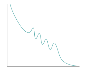
    Refer to caption
    Refer to caption
    Figure 1: The functions g1g_{1} and g4g_{4}

    Let {gn:I⊂ℝ⟶ℝ}\{g_{n}:I\subset\mathbb{R}\longrightarrow\mathbb{R}\} be the family of Morse functions pictured in Figure 1. Denote the Morse cochain complex of gng_{n} over a ring RR by C​M∗​(gn,R)CM^{*}(g_{n};R). Choose continuation maps

    cn:C​M∗​(gn,R)⟶C​M∗​(gn+1,R)c_{n}:CM^{*}(g_{n};R)\longrightarrow CM^{*}(g_{n+1};R)

    that correspond to the inclusion of a subcomplex. Analogously to symplectic cohomology, define a new Morse-type complex

    C​M∗​(g)=⨁n=0∞C​M∗​(gn,R)​[𝐪],CM^{*}(g)=\bigoplus_{n=0}^{\infty}CM^{*}(g_{n};R)[{\bf q}],

    where 𝐪{\bf q} is a formal variable of degree −1-1, satisfying 𝐪2=0{\bf q}^{2}=0. Denoting the Morse differential by ∂M\partial^{M}, the differential on S​C∗​(M)SC^{*}(M) is given by

    ∂(x+y​𝐪)=∂M(x)+(c−i​d)​(y)+∂M(y)​𝐪.\partial(x+y{\bf q})=\partial^{M}(x)+(c-id)(y)+\partial^{M}(y){\bf q}.

    For x∈Crit​(gn)x\in\textnormal{Crit}(g_{n}), define

    𝒜​(x)=gn​(x).{\cal A}(x)=g_{n}(x).

    The assignment 𝒜{\cal A} extends to a valuation on the Morse complex C​M∗​(g)CM^{*}(g) that, in turn, defines a non-Archimedean metric. We use these metrics to define reduced and completed Morse cohomology theories, denoted by H​M∗¯​(g)\overline{HM^{*}}(g) and H​M∗^​(g)\widehat{HM^{*}}(g). It is straight-forward to see that

    H​M∗¯​(g)=0,\overline{HM^{*}}(g)=0,

    but

    H​M∗^​(g)=R.\widehat{HM^{*}}(g)=R.

    For any single gng_{n},

    H​M∗¯​(gn)=H​M∗^​(gn)=0.\overline{HM^{*}}(g_{n})=\widehat{HM^{*}}(g_{n})=0.

    Thus, in this contrived scenario, the reduced cohomology seems to behave stably, while the completed theory does not.

2.4 Rabinowitz Floer homology

Recall that a Liouville cobordism WW is an exact symplectic manifold with contact-type boundary. A boundary component is positive if the contact orientation agrees with the boundary orientation. Otherwise, it is negative. A filled Liouville cobordism is an exact symplectic manifold DD with positive contact boundary such that

  1. 1.

    WW symplectically embeds into DD and

  2. 2.

    under this embedding, the boundary of DD is the positive boundary of WW.

The completed symplectic cohomology of a domain has a natural extension to a theory for filled cobordisms. This theory was first defined in [7] for trivial Liouville cobordism with Liouville filling and extended to general Liouville cobordism with Liouville filling in [8]. The definition was extended by the author to a completed theory in [24]. We briefly recall the construction for a trivial cobordism.

Define a “dual” symplectic homology theory

S​C∗​(HR)=∏n=0∞C​F∗​(−Hn)​[𝒒].SC_{*}(H_{R})=\prod_{n=0}^{\infty}CF^{*}(-H_{n})[\bm{q}].

As with symplectic cohomology, S​C∗​(HR)SC_{*}(H_{R}) admits a filtration by action, given by the chain complexes C​F(a,∞)∗​(Hn)CF^{*}_{(a,\infty)}(H_{n}). Define subcomplexes

S​C∗(a,∞)​(HR)=∏n=0∞C​F(a,∞)∗​(−Hn)​[𝐪]SC_{*}^{(a,\infty)}(H_{R})=\prod_{n=0}^{\infty}CF^{*}_{(a,\infty)}(-H_{n})[{\bf q}]

with homology S​H∗(a,∞)​(HR)SH_{*}^{(a,\infty)}(H_{R}). Action-completed symplectic homology is defined to be

S​H∗^​(HR)=H⁡(lim→aS​C∗(a,∞)​(HR)).\widehat{SH_{*}}(H_{R})=H\left(\lim_{\begin{subarray}{c}\rightarrow\\ a\end{subarray}}SC_{*}^{(a,\infty)}(H_{R})\right).

Let {Hn′}\{H_{n}^{\prime}\} be a family of Hamiltonians corresponding to some radius R′R^{\prime}, and let {Hn}\{H_{n}\}, as always, be a family of Hamiltonians corresponding to some radius RR. We define a map

𝔠^:S​C∗^​(HR′)⟶S​C∗^​(HR),\mathfrak{\widehat{c}}:\widehat{SC_{*}}(H_{R^{\prime}})\longrightarrow\widehat{SC^{*}}(H_{R}),

as follows. There is a map

S​C∗^​(HR′)⟶S​C∗​(HR′)\widehat{SC_{*}}(H_{R^{\prime}})\longrightarrow SC_{*}(H_{R^{\prime}})

that is the direct limit of the inclusion maps

S​C∗(a,∞)​(HR′)↪S​C∗​(HR′)SC_{*}^{(a,\infty)}(H_{R^{\prime}})\hookrightarrow SC_{*}(H_{R^{\prime}})

and a map

S​C∗​(HR′)⟶C​F∗​(−H0′)SC_{*}(H_{R^{\prime}})\longrightarrow CF^{*}(-H_{0}^{\prime})

that is projection onto the first component. Similarly, there is a map

S​C∗​(HR)⟶S​C∗^​(HR)SC^{*}(H_{R})\longrightarrow\widehat{SC^{*}}(H_{R})

that is the inverse limit of the projection maps

S​C∗​(HR)↠S​Ca∗​(HR)SC^{*}(H_{R})\twoheadrightarrow SC^{*}_{a}(H_{R})

and a map

C​F∗​(H0)↪S​C∗​(HR)CF^{*}(H_{0})\hookrightarrow SC^{*}(H_{R})

that is inclusion into the first component. The map 𝔠^\mathfrak{\widehat{c}} is the composition

S​C∗^​(HR′){\lx@inpgf@ignorespaces\widehat{SC_{*}}(H_{R^{\prime}})}S​C∗^​(HR){\lx@inpgf@ignorespaces\widehat{SC^{*}}(H_{R})}S​C∗​(HR′){\lx@inpgf@ignorespaces SC_{*}(H_{R^{\prime}})}S​C∗​(HR){\lx@inpgf@ignorespaces SC^{*}(H_{R})}C​F∗​(−H0′){\lx@inpgf@ignorespaces CF^{*}(-H_{0}^{\prime})}C​F∗​(H0){\lx@inpgf@ignorespaces CF^{*}(H_{0})}𝔠\scriptstyle{\lx@inpgf@ignorespaces\mathfrak{c}}c\scriptstyle{\lx@inpgf@ignorespaces c}

that projects an infinite sum onto the “C​F∗​(−H0′)CF^{*}(-H_{0}^{\prime})” component, maps this component onto C​F∗​(H0)CF^{*}(H_{0}) via continuation, and finally includes into the symplectic cochain complex.

Without loss of generality assume that R′≤RR^{\prime}\leq R. Define the symplectic cohomology of the cobordism [R′,R]×Σ[R^{\prime},R]\times\Sigma to be the cohomology of the cone of 𝔠\mathfrak{c}, the latter written as

S​C∗​([R′,R]×Σ)=C​o​n​e​(𝔠),SC^{*}([R^{\prime},R]\times\Sigma)=Cone(\mathfrak{c}),

and the completed symplectic cohomology to be the cohomology of the cone of 𝔠^\widehat{\mathfrak{c}},

S​C∗^​([R′,R]×Σ)=C​o​n​e​(𝔠^).\widehat{SC^{*}}([R^{\prime},R]\times\Sigma)=Cone(\widehat{\mathfrak{c}}).

Denote these cohomology theories by S​H∗​([R′,R]×Σ)SH^{*}([R^{\prime},R]\times\Sigma), respectively S​H∗^​([R′,R]×Σ)\widehat{SH^{*}}([R^{\prime},R]\times\Sigma).

  • Remark 8)

    If R′>RR^{\prime}>R, we can still follow the above recipe to define a symplectic cohomology theory. We continue to write S​H∗​([R′,R]×Σ)SH^{*}([R^{\prime},R]\times\Sigma), respectively S​H∗^​([R′,R]×Σ)\widehat{SH^{*}}([R^{\prime},R]\times\Sigma). These theories are dual to S​H∗​([R,R′]×Σ)SH^{*}([R,R^{\prime}]\times\Sigma), respectively S​H∗^​([R,R′]×Σ)\widehat{SH^{*}}([R,R^{\prime}]\times\Sigma).

  • Remark 9)

    Note that, a priori,

    H⁡(S​C∗^​(HR))≠S​H∗^​(HR).H\left(\widehat{SC^{*}}(H_{R})\right)\neq\widehat{SH^{*}}(H_{R}).

    The left-hand side is a quotient by im​(∂^)\textnormal{im}(\widehat{\partial}), while the right-hand side is a quotient by im​(∂^)¯\overline{\textnormal{im}(\widehat{\partial})}. In the examples we consider, however, the two will coincide. See Section 5.

  • Remark 10)

    Suppose that EE is exact and Σ⊂E\Sigma\subset E is a convex contact hypersurface as in (10). Σ\Sigma has associated to it a Floer-type invariant called Rabinowitz Floer homology, denoted by R​F​H∗​(Σ)RFH^{*}(\Sigma). Cieliebak-Frauenfelder-Oancea showed in [7] that there is an isomorphism

    H⁡(C​o​n​e​(𝔠))≃R​F​H​(Σ).H\left(Cone(\mathfrak{c})\right)\simeq RFH(\Sigma).

    In the non-exact case, there is a completed version of Rabinowitz Floer homology associated to a contact hypersurface {R}×Σ\{R\}\times\Sigma, which we denote by R​F​H∗^​({R}×Σ)\widehat{RFH^{*}}(\{R\}\times\Sigma). This was first studied by Albers-Kang in [3]. In Section 5 we will give examples of scenarios in which, for R′<R′′<RR^{\prime}<R^{\prime\prime}<R,

    (19) S​H∗^​([R′,R]×Σ)≃R​F​H∗^​({R′′}×Σ).\widehat{SH^{*}}([R^{\prime},R]\times\Sigma)\simeq\widehat{RFH^{*}}(\{R^{\prime\prime}\}\times\Sigma).

    There are maps

    S​H∗^​([R′,R]×Σ)→S​H∗^​([S′,S]×Σ)\widehat{SH^{*}}([R^{\prime},R]\times\Sigma)\rightarrow\widehat{SH^{*}}([S^{\prime},S]\times\Sigma)

    whenever [S′,S]⊂[R′,R][S^{\prime},S]\subset[R^{\prime},R] [8]. We expect the isomorphism (19) to generalize to an isomorphism

    (20) lim→R′<R′′<RS​H∗^​([R′,R]×Σ)≃R​F​H∗^​({R′′}×Σ).\lim_{\begin{subarray}{c}\rightarrow\\ R^{\prime}<R^{\prime\prime}<R\end{subarray}}\widehat{SH^{*}}([R^{\prime},R]\times\Sigma)\simeq\widehat{RFH^{*}}(\{R^{\prime\prime}\}\times\Sigma).

2.5 Morse-Bott Floer theory and cascades

Thus far we have assumed that all periodic orbits are non-degenerate. In the examples considered in this paper, however, all periodic orbits will be transversally non-degenerate, requiring Morse-Bott techniques. We follow the exposition in [6]. Let HH be a Hamiltonian whose orbits are each either constant and non-degenerate or transversally non-degenerate. For each non-constant orbit x∈𝒫⁡(H)x\in{\cal P}(H) choose a generic perfect Morse function fx:S1⟶ℝf_{x}:S^{1}\longrightarrow\mathbb{R}. A choice of Ω\Omega-tame almost-complex structure JJ defines cascades: tuples 𝐮=(cm,um,cm−1,um−1,…,u1,c0){\bf u}=(c_{m},u_{m},c_{m-1},u_{m-1},\dots,u_{1},c_{0}) associated to a sequence of orbits xm,xm−1,…,x0x_{m},x_{m-1},\dots,x_{0} with xm−1,…,x1x_{m-1},\dots,x_{1} non-constant, such that

  1. 1.

    ci∈im​(xi)c_{i}\in\textnormal{im}(x_{i})

  2. 2.

    uiu_{i} is a finite-energy Floer solution corresponding to the Floer data (H,J)(H,J),

  3. 3.

    lims→∞ui​(s,0)\lim\limits_{s\rightarrow\infty}u_{i}(s,0) is in the stable manifold of cic_{i} (or ci=lims→∞ui​(s,t)c_{i}=\lim\limits_{s\rightarrow\infty}u_{i}(s,t) if xix_{i} is constant), and

  4. 4.

    cic_{i} is in the unstable manifold of lims→−∞ui+1​(s,0)\lim\limits_{s\rightarrow-\infty}u_{i+1}(s,0) (or ci=lims→−∞ui+1​(s,t)c_{i}=\lim\limits_{s\rightarrow-\infty}u_{i+1}(s,t) if xix_{i} is constant).

Choose capping discs x~0\tilde{x}_{0} for x0x_{0} and x~m\tilde{x}_{m} for xmx_{m}. The union x~m​#−um​#−um−1​#​…​#−u1​#−x~0\tilde{x}_{m}\#-u_{m}\#-u_{m-1}\#\dots\#-u_{1}\#-\tilde{x}_{0} represents a homology class β∈H2​(E)\beta\in H_{2}(E). Let pp and qq be constant orbits of HH or critical points of some functions fxf_{x} and fx′f_{x^{\prime}}. The moduli space ℳ^β,m​(q,p)\widehat{{\cal M}}_{\beta,m}(q,p) is the space of tuples (cm,um,cm−1,um−1,…,u1,c0)(c_{m},u_{m},c_{m-1},u_{m-1},\dots,u_{1},c_{0}) representing class β\beta such that cmc_{m} is in the stable manifold of pp (or is equal to a constant orbit pp) and c0c_{0} is in the stable manifold of qq (or equal to a constant orbit qq). Each component of ℳ^β,m​(q,p)\widehat{{\cal M}}_{\beta,m}(q,p) carries an ℝm\mathbb{R}^{m} action, induced by the ℝ\mathbb{R}-actions on each Floer trajectory. By Proposition 3.2 in [6],

ℳβ​(q,p):=⨆m≥1ℳ^β,m​(q,p)/ℝm{\cal M}_{\beta}(q,p):=\bigsqcup_{m\geq 1}{\raisebox{1.99997pt}{$\widehat{{\cal M}}_{\beta,m}(q,p)$}\left/\raisebox{-1.99997pt}{$\mathbb{R}^{m}$}\right.}

is a manifold of the expected dimension. The Floer differential now counts

∂f​l(p)=∑|q|−|p|=1β∈π2​(E)∑u∈ℳβ0​(q,p)±T−[Ω]​(β)q,\partial^{fl}(p)=\sum_{\begin{subarray}{c}|q|-|p|=1\\ \beta\in\pi_{2}(E)\end{subarray}}\sum_{u\in{\cal M}^{0}_{\beta}(q,p)}\pm T^{-[\Omega](\beta)}q,

where ℳβ0​(q,p){\cal M}^{0}_{\beta}(q,p) is the zero-dimensional stratum. The continuation maps are similarly modified.

Instead of using cascades, one could just generically perturb the Hamiltonian. However, the S1S^{1}-symmetry of the unperturbed Hamiltonian will be useful in the computations in this paper. Our use of cascades is justified by a result by Bourgeois-Oancea, showing the equivalence of the two approaches.

Theorem 1 (Bourgeois-Oancea: Theorem 3.7 in [6])

If HH is a transversally-nondegenerate Hamiltonian, there exists a non-degenerate Hamiltonian H′H^{\prime} – a perturbation of HH – such that

C​F∗​(H)≃C​F∗​(H′)CF^{*}(H)\simeq CF^{*}(H^{\prime})

are chain-isomorphic.

3 Negative line bundles

Let (M,ω)(M,\omega) be a symplectic manifold of dimension 2​m−22m-2. Denote by E→𝜌ME\xlongrightarrow{\rho}M the line bundle satisfying c1E=−k⁡[ω]c_{1}^{E}=-k[\omega] for some fixed k>0k>0. Such a line bundle is called negative. EE is a symplectic manifold; assume that EE is weak+ monotone so that moduli spaces of Floer solutions do not see bubbling. Following [16] and [17], we construct a canonical symplectic form on EE through ω\omega.

Let JJ be an ω\omega-compatible almost-complex structure on MM. Let |⋅||\cdot| be a Hermitian metric on EE with induced Chern curvature ℱ{\cal F}. Define a radial coordinate rr by r⁡(w)=|w|r(w)=|w| and a fiber-wise angular one-form on the complement of the zero-section by

α=14​π​k​dc​log⁡(r2)\alpha=\frac{1}{4\pi k}d^{c}\log(r^{2})

so that

d​α=14​π​k​d​dc​log⁡(r2)=i2​π​k​∂∂¯​log⁡(r2)=−i2​π​k​ρ∗​ℱ≡−1k​ρ∗​c1E≡ρ∗​[ω].d\alpha=\frac{1}{4\pi k}dd^{c}\log(r^{2})=\frac{i}{2\pi k}\partial\bar{\partial}\log(r^{2})=-\frac{i}{2\pi k}\rho^{*}{\cal F}\equiv-\frac{1}{k}\rho^{*}c_{1}^{E}\equiv\rho^{*}[\omega].

Note that α\alpha defines a contact one-form on the unit circle bundle. Let

Ω:=(1+k​π​r2)​d​α+2​k​π​r​d​r∧α=d​α+d⁡(k​π​r2​α)\Omega:=(1+k\pi r^{2})d\alpha+2k\pi rdr\wedge\alpha=d\alpha+d(k\pi r^{2}\alpha)

be a symplectic form on the complement of the zero section. Extend Ω\Omega smoothly over the zero-section by

Ω|zero section=−i2​π​k​ρ∗​ℱ+{area form of fiber}.\Omega\big|_{\text{zero section}}=-\frac{i}{2\pi k}\rho^{*}{\cal F}+\text{\lx@text@lbrace area form of fiber\lx@text@rbrace}.

Then Ω\Omega is a symplectic form on EE and [Ω]=[ρ∗​ω][\Omega]=[\rho^{*}\omega].

We wish to compute the symplectic cohomology of EE. There is a simple family of Hamiltonians to take, which lead to an elegant computation of S​H∗​(E)SH^{*}(E). This was developed by Ritter in [17] and [18] using the S1S^{1}-action on EE that rotates the fibers. To fit our framework, we modify this construction slightly, and we appeal to [11] to assert that the two frameworks yield isomorphic homology theories.

Let {gn:ℝ⟶ℝ}n∈ℤ\{g_{n}:\mathbb{R}\longrightarrow\mathbb{R}\}_{n\in\mathbb{Z}} be a family of functions defined as

gn​(r)=(nk+12​k)​r,g_{n}(r)=\left(\frac{n}{k}+\frac{1}{2k}\right)r,

as depicted in Figure 2. Choose a 𝒞2{\cal C}^{2}-small Morse function f:M⟶ℝf:M\longrightarrow\mathbb{R} on MM. Define

Gn=gn​(k​π​r2)+(1+k​π​r2)​ρ∗​f.G_{n}=g_{n}(k\pi r^{2})+(1+k\pi r^{2})\rho^{*}f.
ℝ\mathbb{R}k​π​r2k\pi r^{2}g0g_{0}g1g_{1}g2g_{2}
Figure 2: The Hamiltonians g0​(k​π​r2),g1​(k​π​r2),g_{0}(k\pi r^{2}),g_{1}(k\pi r^{2}), and g2​(k​π​r2)g_{2}(k\pi r^{2})

Recall that, away from the zero section,

Ω=(1+k​π​r2)​d​α+2​k​π​r​d​r∧α\Omega=(1+k\pi r^{2})d\alpha+2k\pi rdr\wedge\alpha

Let XfhX_{f}^{h} be the horizontal lift of the Hamiltonian vector field XfX_{f} on MM, uniquely defined through the connection one-form α\alpha. As

d​Gn\displaystyle dG_{n} =2​k​π​r​(gn′​(k​π​r2)+ρ∗​f)​d​r+(1+k​π​r2)​ρ∗​d​f\displaystyle=2k\pi r(g_{n}^{\prime}(k\pi r^{2})+\rho^{*}f)dr+(1+k\pi r^{2})\rho^{*}df
=2​k​π​r​(nk+12​k+ρ∗​f)​d​r+(1+k​π​r2)​ρ∗​d​f,\displaystyle=2k\pi r\left(\frac{n}{k}+\frac{1}{2k}+\rho^{*}f\right)dr+(1+k\pi r^{2})\rho^{*}df,

the Hamiltonian vector field of GnG_{n} away from the zero section is

XGn=(nk+12​k+ρ∗​f)​Rα+Xfh.X_{G_{n}}=\left(\frac{n}{k}+\frac{1}{2k}+\rho^{*}f\right)R_{\alpha}+X_{f}^{h}.

The Reeb orbits of α\alpha have period 1k\frac{1}{k}, and so the periodic orbits of XGnX_{G_{n}} exist only where nk+12​k+ρ∗​f\frac{n}{k}+\frac{1}{2k}+\rho^{*}f is an integer multiple of 1k\frac{1}{k}. By construction, ρ∗​f\rho^{*}f is 𝒞2{\cal C}^{2}-small, and so we can assume that XGnX_{G_{n}} has no periodic orbits away from the zero section. On the zero section XGn=XfhX_{G_{n}}=X_{f}^{h}, which can be identified with XfX_{f}. Thus, the periodic orbits of XGnX_{G_{n}} correspond to the periodic orbits of XfX_{f}. As ff is 𝒞2{\cal C}^{2} small, these correspond precisely to the critical points of the Morse function ff. It follows that there is a vector space isomorphism

C​F∗​(Gn)≃C​M∗​(f)CF^{*}(G_{n})\simeq CM^{*}(f)

for every n∈ℤn\in\mathbb{Z}.

Suppose that σ:S1⟶H​a​m​(E,i​d)\sigma:S^{1}\longrightarrow Ham(E,id) is a loop of Hamiltonians based at the identity. Then σ\sigma acts on the loopspace ℒ⁡(E){\cal L}(E) by σ∗​x​(t)=σ⁡(t)​(x⁡(t))\sigma^{*}x(t)=\sigma(t)(x(t)). This lifts to an action σ~\tilde{\sigma} on a cover of the loopspace ℒ⁡(E)~\widetilde{{\cal L}(E)}. We fix ℒ⁡(E)~\widetilde{{\cal L}(E)} to be the cover defined by the deck transformation group

Γ=ker⁡([Ω]|π2​(E))∩ker⁡(c1T​E​(E)|π2​(E)).\Gamma=\ker([\Omega]\big|_{\pi_{2}(E)})\cap\ker(c_{1}^{TE}(E)\big|_{\pi_{2}(E)}).

In other words, ℒ⁡(E)~\widetilde{{\cal L}(E)} is the group of cappings of each loop, under the equivalence relation u≃vu\simeq v if

  • •

    ∂u=∂v\partial u=\partial v,

  • •

    [Ω]​([u​#​(−v)])=0[\Omega]([u\#(-v)])=0, and

  • •

    c1T​E​([u​#​(−v)])=0c_{1}^{TE}([u\#(-v)])=0.

Let σt\sigma_{t} be the action on EE that rotates each fiber by e2​π​i​te^{2\pi it}. This is a Hamiltonian action generated by the Hamiltonian 1k​(k​π​r2)\frac{1}{k}(k\pi r^{2}), preserving the radial coordinate k​π​r2k\pi r^{2}, and so

σt∗​Gn:=Gn∘σt−(1k​k​π​r2)∘σt=(Gn−1k​(k​π​r2))∘σt=Gn−1.\sigma_{t}^{*}G_{n}:=G_{n}\circ\sigma_{t}-\left(\frac{1}{k}k\pi r^{2}\right)\circ\sigma_{t}=\left(G_{n}-\frac{1}{k}(k\pi r^{2})\right)\circ\sigma_{t}=G_{n-1}.

Define the lift σ~\tilde{\sigma} to preserve cappings of constant loops.

Let JtJ_{t} be any one-parameter family of Ω\Omega-tame almost-complex structures. The action of σt\sigma_{t} on JtJ_{t} defined by

σt∗​Jt=d​σt−1∘Jt∘d​σt,\sigma_{t}^{*}J_{t}=d\sigma_{t}^{-1}\circ J_{t}\circ d\sigma_{t},

produces another one-parameter family of Ω\Omega-tame almost complex structures. Recall that Floer data (H,J)(H,J) is generic if the Floer cochain complex C​F∗​(H,J)CF^{*}(H,J) is well-defined. The following two theorems, due to Ritter, yield the promised computation of symplectic cohomology (see Section 7 of [17]).

Theorem 5 (Ritter [17])

If (Gn,J)(G_{n},J) is generic, then so is (σt∗​Gn,σt∗​J)(\sigma_{t}^{*}G_{n},\sigma_{t}^{*}J). The action σ~\tilde{\sigma} induces a chain isomorphism

𝒮:C​F∗​(Gn,J)⟶C​F∗+2​(σ∗​Gn,σ∗​J)=C​F∗+2​(Gn−1,σ∗​J).{\cal S}:CF^{*}(G_{n},J)\longrightarrow CF^{*+2}(\sigma^{*}G_{n},\sigma^{*}J)=CF^{*+2}(G_{n-1},\sigma^{*}J).

Choose continuation maps

cnG:C​F∗​(Gn,J)⟶C​F∗​(Gn+1,J′)c^{G}_{n}:CF^{*}(G_{n},J)\longrightarrow CF^{*}(G_{n+1},J^{\prime})

between Floer data (Gn,J)(G_{n},J) and (Gn+1,J′)(G_{n+1},J^{\prime}).

Theorem 6 (Ritter [17])

The following diagram induces a commutative diagram on the level of cohomology.

C​F∗​(Gn−1,J){\lx@inpgf@ignorespaces CF^{*}(G_{n-1},J)}C​F∗​(Gn,J′){\lx@inpgf@ignorespaces CF^{*}(G_{n},J^{\prime})}C​F∗+2​n​(G−1,(σ∗)n​J){\lx@inpgf@ignorespaces CF^{*+2n}(G_{-1},(\sigma^{*})^{n}J)}C​F∗+2​n​(G0,(σ∗)n​J′){\lx@inpgf@ignorespaces CF^{*+2n}(G_{0},(\sigma^{*})^{n}J^{\prime})}cn−1G\scriptstyle{\lx@inpgf@ignorespaces c_{n-1}^{G}}𝒮n\scriptstyle{\lx@inpgf@ignorespaces{\cal S}^{n}}𝒮n\scriptstyle{\lx@inpgf@ignorespaces{\cal S}^{n}}c−1G\scriptstyle{\lx@inpgf@ignorespaces c_{-1}^{G}}
Corollary 2 (Ritter [17])

The symplectic cochain complex

S​C∗​(G):=⨁n=0∞C​F∗​(Gn)​[𝐪]SC^{*}(G):=\bigoplus_{n=0}^{\infty}CF^{*}(G_{n})[{\bf q}]

is quasi-isomorphic to a complex

S​C∗​(G0):=⨁n=0∞C​F∗​(G0)​[−2​n]​[𝐪]SC^{*}(G_{0}):=\bigoplus_{n=0}^{\infty}CF^{*}(G_{0})[-2n][{\bf q}]

with differential

∂(x+y​𝐪)=∂f​l(x)+y−c−1G∘𝒮⁡(y)+∂f​l(y)​𝐪.\partial(x+y{\bf q})=\partial^{fl}(x)+y-c_{-1}^{G}\circ{\cal S}(y)+\partial^{fl}(y){\bf q}.

Note that the grading shift [−2​n][-2n] increases the Conley-Zehnder index by 2​n2n.

Denote the 00th generalized eigenspace of the map

𝒄−𝟏𝑮∘𝒮:HF∗(H0)⟶HF(H0).\bm{c_{-1}^{G}}\circ\bm{{\cal S}}:HF^{*}(H_{0})\longrightarrow HF^{(}H_{0}).

by H​F0∗​(H0)HF^{*}_{0}(H_{0}). A linear algebra consequence of Corollary 2 is

Corollary 3 (Ritter [17])

The uncompleted symplectic cohomology of EE is

S​H∗​(E)=S​H∗​(G)≅S​H∗​(G0)≅H​F∗​(H0)/H​F0∗​(H0).SH^{*}(E)=SH^{*}(G)\cong SH^{*}(G_{0})\cong{\raisebox{2.04439pt}{$HF^{*}(H_{0})$}\left/\raisebox{-2.04439pt}{$HF^{*}_{0}(H_{0})$}\right.}.

Under this isomorphism, the map

H​F∗​(H0)⟶S​H∗​(E)HF^{*}(H_{0})\longrightarrow SH^{*}(E)

induced by inclusion on cochains is the quotient map.

Finally, symplectic cohomology can be rephrased completely in terms of topological information. There is a map, termed the P.S.S. map after its creators Piukhin-Salamon-Schwartz, that identifies the quantum cohomology Q​H∗​(E)QH^{*}(E) with H​F∗​(H0)HF^{*}(H_{0}).

Theorem 7 (Ritter [17])

The P.S.S. isomorphism

Q​H∗​(E)≅H​F∗​(H0)QH^{*}(E)\cong HF^{*}(H_{0})

identifies up to non-zero scalar η\eta the map 𝐜−𝟏𝐆∘𝒮\bm{c_{-1}^{G}}\circ\bm{{\cal S}} with the action of quantum cup product ∪∗\cup_{*} with ρ∗​c1E\rho^{*}c_{1}^{E}. If Q​H0∗​(E)QH^{*}_{0}(E) is the 00th-generalized eigenspace of the map x↦ρ∗c1E∪∗xx\mapsto\rho^{*}c_{1}^{E}\cup_{*}x, there is an isomorphism of Λ\Lambda-algebras

S​H∗​(E)≅Q​H∗​(E)/Q​H0∗​(E).SH^{*}(E)\cong{\raisebox{2.04439pt}{$QH^{*}(E)$}\left/\raisebox{-2.04439pt}{$QH^{*}_{0}(E)$}\right.}.

Indeed, Ritter shows that the scalar η\eta has valuation e​v​(η)=0ev(\eta)=0 (see Theorem 67 of [17]).

Corollary 4

The P.S.S. isomorphism identifies a λ\lambda-generalized eigenspace of 𝐜−𝟏𝐆∘𝒮−𝟏\bm{c_{-1}^{G}}\circ\bm{{\cal S}^{-1}} with a η​λ\eta\lambda-generalized eigenspace of ρ∗c1E∪∗−\rho^{*}c_{1}^{E}\cup_{*}-, and

e​v​(λ)=e​v​(η​λ).ev(\lambda)=ev(\eta\lambda).

3.1 Disk subbundles

We now use reduced symplectic cohomology to define an invariant of a disk subbundle contained in EE. Fix a radius R∈(0,∞)R\in(0,\infty), and let DRD_{R} be the disk bundle of radius RR. Following Subsection 2.2, we will construct a chain complex generated by one-periodic orbits that cluster near the boundary of DRD_{R}. With an eye towards computing reduced symplectic cohomology, we use a specific family of Hamiltonians and a specific class of almost-complex structures.

3.1.1 The almost-complex structure

Let 𝒥⁡(ωs​t​d){\cal J}(\omega_{std}) be the space of S1S^{1}-families of almost-complex structures on ℂ\mathbb{C} compatible with the standard symplectic form, and such that each almost-complex structure is cylindrical in a neighborhood of periodic orbits and at infinity. Let 𝒥⁡(ω){\cal J}(\omega) be the space of S1S^{1}-families of almost-complex structures on MM compatible with ω\omega. The one-form α\alpha determines a splitting of T​ETE into a vertical component V≅ℂV\cong\mathbb{C} and horizontal component HH. Let Lt​(H,V)L_{t}(H,V) be the space of S1S^{1}-families of linear maps from HH to VV. Let 𝒰{\cal U} be an open set comprised of small neighborhoods of the circle bundles on which live non-constant periodic orbits of each HnH_{n}, as well as small neighborhoods of the constant orbits. Let 𝔅⁡(it,jt)\mathfrak{B}(i_{t},j_{t}) be the elements Bt∈Lt​(H,V)B_{t}\in L_{t}(H,V) with compact support in the complement of 𝒰{\cal U}, and satisfying it​Bt+Bt​ρ∗​jt=0i_{t}B_{t}+B_{t}\rho^{*}j_{t}=0 for all tt. Define

𝒥(Ω)={Jt=[itBt0ρ∗​jt]∈End(TE)|it∈𝒥(ωs​t​d),jt∈𝒥(ω),Bt∈𝔅(it,jt),Jt is Ω–tame}.{\cal J}(\Omega)=\left\{J_{t}=\left[\begin{array}[]{cc}i_{t}&B_{t}\\ 0&\rho^{*}j_{t}\end{array}\right]\in End(TE)\hskip 2.84544pt\bigg|\hskip 2.84544pti_{t}\in{\cal J}(\omega_{std}),j_{t}\in{\cal J}(\omega),B_{t}\in\mathfrak{B}(i_{t},j_{t}),J_{t}\text{ is }\Omega\text{--tame}\right\}.

The conditions on it,jti_{t},j_{t} and BtB_{t} ensure that Floer trajectories “flow outward”, that Floer trajectories converge to periodic orbits, and that JtJ_{t} is almost-complex.

Transversality and regularity for J∈𝒥⁡(Ω)J\in{\cal J}(\Omega) was proven by Albers-Kang in [3] for the completely analogous case of Floer solutions in Rabinowitz Floer homology. We therefore omit these proofs, and simply refer to [3].

Lemma 1 (Albers-Kang: Proposition 2.11 in [3]))

There exists a comeager subset of 𝒥⁡(Ω){\cal J}(\Omega) for which the finite-energy cascades of HnH_{n} and HnsH_{n}^{s}, for any nn, are cut out transversally.

Lemma 2 (Albers-Kang: Lemma 2.15 in [3])

All simple JJ-holomorphic spheres are regular.

3.1.2 The Hamiltonians

Fix a constant C>0C>0 and let {hn:ℝ⟶ℝ}n∈ℕ\left\{h_{n}\colon\mathbb{R}\longrightarrow\mathbb{R}\right\}_{n\in\mathbb{N}} be a family of functions where each hnh_{n} is

  1. 1.

    convex and monotone increasing on ℝ≥0\mathbb{R}_{\geq 0},

  2. 2.

    bounded in absolute value by CC on [0,k​π​R2][0,k\pi R^{2}], and

  3. 3.

    of slope nk+12​k\frac{n}{k}+\frac{1}{2k} on (k​π​Rn2,∞)(k\pi R_{n}^{2},\infty), for some Rn<RR_{n}<R.

Further assume that the sequence {Rn}\{R_{n}\} tends to RR as nn tends to ∞\infty. To simplify later proofs, we also choose hnh_{n} such that

  1. 1.

    hnh_{n} and hn′h_{n}^{\prime} are monotone increasing on ℝ≥0\mathbb{R}_{\geq 0} and

  2. 2.

    hn=hn+1h_{n}=h_{n+1} on [0,k​π​Rn2][0,k\pi R_{n}^{2}].

For example, we can take {hn}\{h_{n}\} to be smoothings of the functions shown in Figure 3.

Choose a Morse function function f:M⟶ℝf\colon M\longrightarrow\mathbb{R} that is 𝒞2{\cal C}^{2}-small. Define a family of Hamiltonians {Hn:E⟶ℝ}n∈ℕ\left\{H_{n}\colon E\longrightarrow\mathbb{R}\right\}_{n\in\mathbb{N}} by

Hn=hn​(k​π​r2)+(1+k​π​r2)​ρ∗​f.H_{n}=h_{n}(k\pi r^{2})+(1+k\pi r^{2})\rho^{*}f.

We assume that the one-periodic orbits of HnH_{n} are transversally nondegenerate. For example, we can take each hnh_{n} to be a smoothing of a piecewise linear function, as in Figure 3.

ℝ\mathbb{R}k​π​r2k\pi r^{2}h0h_{0}h1h_{1}h2h_{2}h3h_{3}...
Figure 3: A family of Hamiltonians {hn​(k​π​r2)}\{h^{n}(k\pi r^{2})\}

Let RαR_{\alpha} be the unique vector field on E∖{zero section}E\setminus\{\text{zero section}\} satisfying

{α⁡(Rα)=1d​r​(Rα)=0iRα​d​α=0.\left\{\begin{array}[]{c}\alpha(R_{\alpha})=1\\ dr(R_{\alpha})=0\\ i_{R_{\alpha}}d\alpha=0\end{array}\right..

Note that Rα|r=𝔯R_{\alpha}\big|_{r=\mathfrak{r}} is the Reeb vector field of the contact form α|{r=𝔯}\alpha\big|_{\{r=\mathfrak{r}\}} and the simply-covered orbits of RαR_{\alpha} have period 1k\frac{1}{k}. As

d​Hn=2​k​π​r​(hn′​(k​π​r2)+ρ∗​f)​d​r+(1+k​π​r2)​ρ∗​d​f,dH_{n}=2k\pi r(h_{n}^{\prime}(k\pi r^{2})+\rho^{*}f)dr+(1+k\pi r^{2})\rho^{*}df,

the Hamiltonian vector field of HnH_{n} is

XHn=(hn′​(k​π​r2)+ρ∗​f)​Rα+Xfh,X_{H_{n}}=(h_{n}^{\prime}(k\pi r^{2})+\rho^{*}f)R_{\alpha}+X_{f}^{h},

Thus, the one-periodic orbits of HnH_{n} correspond bijectively to

  1. 1.

    the S1S^{1}-families of orbits of Rα|DRR_{\alpha}\big|_{D_{R}} with period between 1k\frac{1}{k} and 1n\frac{1}{n}, lying in fibers above the critical points of ff, and

  2. 2.

    the critical points of ff itself.

Impose a perfect Morse function on each S1S^{1}-family of orbits, so that each family gives rise to two distinguished orbits: the minimum and the maximum of the perfect Morse function.

Denote by 𝒫⁡(Hn){\cal P}(H_{n}) the union of all minimum and maximum distinguished orbits of HnH_{n}, in addition to the constant orbits, and by 𝒫⁡(H){\cal P}(H) the union ⋃n𝒫⁡(Hn)\bigcup\limits_{n}{\cal P}(H_{n}).

Choose generic almost-complex structures in 𝒥⁡(Ω){\cal J}(\Omega) to define the Floer complexes C​F∗​(Hn)CF^{*}(H_{n}). For each nn choose a generic ℝ\mathbb{R}-family of functions hns:ℝ→ℝh_{n}^{s}\colon\mathbb{R}\rightarrow\mathbb{R}, monotonely decreasing in ss, with hns=hnh_{n}^{s}=h_{n} when s>>0s>>0 and hns=hn+1h_{n}^{s}=h_{n+1} when s<<0s<<0. Set Hns=hns​(k​π​r2)+(1+k​π​r2)​ρ∗​fH_{n}^{s}=h_{n}^{s}(k\pi r^{2})+(1+k\pi r^{2})\rho^{*}f. Define continuation maps

cn:C​F∗​(Hn)→C​F∗​(Hn+1)c_{n}:CF^{*}(H_{n})\rightarrow CF^{*}(H_{n+1})

through HnsH_{n}^{s}. In the notation of Section 2, this collection of data defines cochain complexes S​C∗​(H),S​C∗¯​(H),SC^{*}(H),\overline{SC^{*}}(H), and S​C∗^​(H)\widehat{SC^{*}}(H).

3.1.3 Some technical lemmas for computation

In order to compute S​H∗¯​(H)\overline{SH^{*}}(H), we need three standard results on the behavior of the Floer differential and continuation maps.

Define 𝔴⁡(x)\mathfrak{w}(x) to be the winding number of a non-constant periodic orbit xx, viewed as a map from the circle into ℂ∗\mathbb{C}^{*}. Define 𝔴⁡(x)\mathfrak{w}(x) of a constant orbit xx to be zero.

Lemma 3

Let uu be a solution of Floer’s equation (8) with lims→±∞u⁡(s,t)=x±​(t)\lim\limits_{s\rightarrow\pm\infty}u(s,t)=x_{\pm}(t). Then 𝔴⁡(x+)≥𝔴⁡(x−)\mathfrak{w}(x_{+})\geq\mathfrak{w}(x_{-}).

Proof.

We use the integrated maximum principal of [1]. Assume for contradiction that 𝔴⁡(x−)>𝔴⁡(x+)\mathfrak{w}(x_{-})>\mathfrak{w}(x_{+}). Say that x±x_{\pm} lives in the sphere bundle of radius σ±\sigma_{\pm}. If x±x_{\pm} are non-constant then the RαR_{\alpha}-orbit underlying x±x_{\pm} has period 1k​𝔴​(x±)\frac{1}{k}\mathfrak{w}(x_{\pm}). From the earlier computation XHn=(hn′​(k​π​r2)+ρ∗​f)​Rα+XfhX_{H_{n}}=(h_{n}^{\prime}(k\pi r^{2})+\rho^{*}f)R_{\alpha}+X_{f}^{h} it follows that hn′​(k​π​σ±2)+ρ∗​f​(x±)=1k​𝔴​(x±)h_{n}^{\prime}(k\pi\sigma_{\pm}^{2})+\rho^{*}f(x_{\pm})=\frac{1}{k}\mathfrak{w}(x_{\pm}). The winding numbers are integers, and so

hn′​(k​π​σ−2)+ρ∗​f​(x−)≥hn′​(k​π​σ+2)+ρ∗​f​(x+)+1k.h_{n}^{\prime}(k\pi\sigma_{-}^{2})+\rho^{*}f(x_{-})\geq h_{n}^{\prime}(k\pi\sigma_{+}^{2})+\rho^{*}f(x_{+})+\frac{1}{k}.

By the smallness of ff we can assume that

hn′​(k​π​σ−2)−hn′​(k​π​σ+2)≥ρ∗​f​(x+)−ρ∗​f​(x−)+1k>0.h_{n}^{\prime}(k\pi\sigma_{-}^{2})-h_{n}^{\prime}(k\pi\sigma_{+}^{2})\geq\rho^{*}f(x_{+})-\rho^{*}f(x_{-})+\frac{1}{k}>0.

As hnh_{n} is convex, we deduce that σ−>σ+\sigma_{-}>\sigma_{+}. If x+x_{+} is constant and x−x_{-} is non-constant it follows immediately that σ−>σ+=0\sigma_{-}>\sigma_{+}=0.

Choose a generic circle subbundle 𝔖\mathfrak{S} of radius σ\sigma, with σ+<σ<σ−\sigma_{+}<\sigma<\sigma_{-}, and on which B=0B=0 and iti_{t} is cylindrical. For example, if σ\sigma is close to σ+\sigma_{+} or σ−\sigma_{-} these conditions will, by construction, be met. Let 𝒟{\cal D} be the region bounded by 𝔖\mathfrak{S}, and denote Σ=u−1​(E∖𝒟)\Sigma=u^{-1}(E\setminus{\cal D}). Let v:Σ⟶E∖𝒟v\colon\Sigma\longrightarrow E\setminus{\cal D} be the restriction of uu. We will equate Σ\Sigma with its image under the inclusion into ℝ×S1\mathbb{R}\times S^{1} and use the coordinates (s,t)(s,t) induced on Int​(Σ)\textnormal{Int}(\Sigma).

Let cx=hn​(k​π​x2)−hn′​(k​π​x2)​k​π​x2c_{x}=h_{n}(k\pi x^{2})-h^{\prime}_{n}(k\pi x^{2})k\pi x^{2} be the yy-intercept of the tangent line to hn​(k​π​r2)h_{n}(k\pi r^{2}) at k​π​x2k\pi x^{2}. Then on 𝔖\mathfrak{S}, Hn=hn′​(k​π​σ2)​k​π​σ2+(1+k​π​σ2)​ρ∗​f+cσH_{n}=h_{n}^{\prime}(k\pi\sigma^{2})k\pi\sigma^{2}+(1+k\pi\sigma^{2})\rho^{*}f+c_{\sigma} (and XHn=(hn′​(k​π​σ2)+ρ∗​f)​Rα+XfhX_{H_{n}}=(h_{n}^{\prime}(k\pi\sigma^{2})+\rho^{*}f)R_{\alpha}+X_{f}^{h}). In particular,

Hn|𝔖=(1+k​π​σ2)​α​(XHn)−hn′​(k​π​σ2)+cσ.H_{n}\big|_{\mathfrak{S}}=(1+k\pi\sigma^{2})\alpha(X_{H_{n}})-h_{n}^{\prime}(k\pi\sigma^{2})+c_{\sigma}.

Let ∂Σ+\partial\Sigma_{+} be the union of the boundary components of Σ\Sigma mapping into 𝔖\mathfrak{S}. Note that we have chosen JJ to be Ω\Omega-tame, so that

EJ​(v):=12​∫Σ(Ω⁡(∂sv,J​∂sv)+Ω⁡(∂tv−XHn​(v),J⁡(∂tv−XHn​(v)))​𝑑s∧𝑑t≥0CLOSEE_{J}(v):=\frac{1}{2}\int_{\Sigma}\left(\Omega(\partial_{s}v,J\partial_{s}v\right)+\Omega\left(\partial_{t}v-X_{H_{n}}(v),J(\partial_{t}v-X_{H_{n}}(v))\right)ds\wedge dt\geq 0

Shuffling terms, we have

EJ​(v)=∫Σv∗​Ω−v∗​d​Hn⊗𝑑t=∫∂Σ+(1+k​π​r2)​v∗​α−Hn​(v⁡(s,t))​𝑑t−∫S1(1+k​π​r2)​x−∗​α−Hn​(x−​(t))​𝑑t=∫∂Σ+(1+k​π​σ2)​v∗​α−(1+k​π​σ2)​α​(XHn)⊗𝑑t+(hn′​(k​π​σ2)−cσ)​𝑑t−∫S1(1+kπσ−2)x−∗α−Hn(x−(t))dt\begin{split}E_{J}(v)&=\int_{\Sigma}v^{*}\Omega-v^{*}dH_{n}\otimes dt\\ &=\int_{\partial\Sigma_{+}}(1+k\pi r^{2})v^{*}\alpha-H_{n}(v(s,t))dt-\int_{S^{1}}(1+k\pi r^{2})x_{-}^{*}\alpha-H_{n}(x_{-}(t))dt\\ &=\int_{\partial\Sigma_{+}}(1+k\pi\sigma^{2})v^{*}\alpha-(1+k\pi\sigma^{2})\alpha(X_{H_{n}})\otimes dt+\left(h^{\prime}_{n}(k\pi\sigma^{2})-c_{\sigma}\right)dt\\ &\hskip 56.9055pt-\int_{S^{1}}(1+k\pi\sigma_{-}^{2})x_{-}^{*}\alpha-H_{n}(x_{-}(t))dt\end{split}

We consider this final equation in pieces. A solution v⁡(s,t)v(s,t) of Floer’s equation satisfies

(d​v−XHn⊗d​t)(0,1)=0.(dv-X_{H_{n}}\otimes dt)^{(0,1)}=0.

We have that, on 𝔖\mathfrak{S}, d​r∘it=−2​k​π​r​αdr\circ i_{t}=-2k\pi r\alpha and Bt=0B_{t}=0. The former implies that J​RαJR_{\alpha} is proportional to ∂r\partial_{r} and the latter implies that J​XfhJX_{f}^{h} lives in the horizontal distribution. So altogether, α⁡(J​XHn)=0\alpha(JX_{H_{n}})=0. Thus, the “∂Σ+\partial\Sigma_{+}” terms become

∫∂Σ+(1+k​π​σ2)​α​(𝑑v−XHn⊗𝑑t)+\displaystyle\int_{\partial\Sigma_{+}}(1+k\pi\sigma^{2})\alpha(dv-X_{H_{n}}\otimes dt)+ (hn′​(k​π​σ2)−cσ)​d​t\displaystyle\left(h^{\prime}_{n}(k\pi\sigma^{2})-c_{\sigma}\right)dt
=∫∂Σ+−(1+kπσ2)α∘J(dv−XHn⊗dt)∘j+(hn′(kπσ2)−cσ)dt\displaystyle=\int_{\partial\Sigma_{+}}-(1+k\pi\sigma^{2})\alpha\circ J(dv-X_{H_{n}}\otimes dt)\circ j+\left(h^{\prime}_{n}(k\pi\sigma^{2})-c_{\sigma}\right)dt
=∫∂Σ+−1+k​π​σ22​k​π​σdr∘dv∘j+(hn′(kπσ2)−cσ)dt\displaystyle=\int_{\partial\Sigma_{+}}-\frac{1+k\pi\sigma^{2}}{2k\pi\sigma}dr\circ dv\circ j+\left(h^{\prime}_{n}(k\pi\sigma^{2})-c_{\sigma}\right)dt
≤∫∂Σ+(hn′​(k​π​σ2)−cσ)​𝑑t,\displaystyle\leq\int_{\partial\Sigma_{+}}\left(h^{\prime}_{n}(k\pi\sigma^{2})-c_{\sigma}\right)dt,

where the last inequality follows because a vector ζ\zeta that is positively-oriented with respect to the boundary orientation satisfies d​r∘j⁡(ζ)≥0dr\circ j(\zeta)\geq 0. We also have

Hn​(x−​(t))=hn′​(k​π​σ−2)​k​π​σ−2+cσ−+(1+k​π​σ−2)​ρ∗​f​(x−​(t))=(1+k​π​σ−2)​𝔴⁡(x−)k−hn′​(k​π​σ2)+cσ−H_{n}(x_{-}(t))=h_{n}^{\prime}(k\pi\sigma_{-}^{2})k\pi\sigma_{-}^{2}+c_{\sigma_{-}}+(1+k\pi\sigma_{-}^{2})\rho^{*}f(x_{-}(t))=(1+k\pi\sigma_{-}^{2})\frac{\mathfrak{w}(x_{-})}{k}-h_{n}^{\prime}(k\pi\sigma^{2})+c_{\sigma_{-}}

and so the “x−x_{-}” terms become

−∫S1(1+kπr2)x−∗α+∫01Hn(x−(t))dt\displaystyle-\int_{S^{1}}(1+k\pi r^{2})x_{-}^{*}\alpha+\int_{0}^{1}H_{n}(x_{-}(t))dt =−𝔴⁡(x−)k​(1+k​π​σ−2)+𝔴⁡(x−)k​(1+k​π​σ−2)+cσ−−hn′​(k​π​σ−2)\displaystyle=-\frac{\mathfrak{w}(x_{-})}{k}(1+k\pi\sigma_{-}^{2})+\frac{\mathfrak{w}(x_{-})}{k}(1+k\pi\sigma_{-}^{2})+c_{\sigma_{-}}-h_{n}^{\prime}(k\pi\sigma^{2}_{-})
=∫S1(−hn′​(k​π​σ−2)+cσ−)​𝑑t\displaystyle=\int_{S^{1}}\left(-h_{n}^{\prime}(k\pi\sigma_{-}^{2})+c_{\sigma_{-}}\right)dt

Altogether,

(21) EJ​(v)\displaystyle E_{J}(v) ≤∫∂Σ+(hn′​(k​π​σ2)−cσ)​𝑑t+∫S1(−hn′​(k​π​σ−2)+cσ−)​𝑑t.\displaystyle\leq\int_{\partial\Sigma_{+}}\left(h^{\prime}_{n}(k\pi\sigma^{2})-c_{\sigma}\right)dt+\int_{S^{1}}\left(-h_{n}^{\prime}(k\pi\sigma_{-}^{2})+c_{\sigma_{-}}\right)dt.

Σ\Sigma is a collection of bounded regions in ℂ∗\mathbb{C}^{*} and one unbounded region enclosing the origin. As d​tdt is exact on ℂ∗\mathbb{C}^{*}, the bounded regions contribute nothing to the right-hand side of (21). Let Σ~\tilde{\Sigma} be the unbounded component. Near zero, Σ\Sigma is contained in a neighborhood of x−x_{-}, and so all boundary components of Σ~\tilde{\Sigma} occur within the intersection of Σ\Sigma with some annulus [R,∞)×S1[R,\infty)\times S^{1}. Let 𝔥\mathfrak{h} be a function on Σ~\tilde{\Sigma} that is equal to hn′​(k​π​σ2)−cσh_{n}^{\prime}(k\pi\sigma^{2})-c_{\sigma} on Σ~∩([R,∞)×S1)\tilde{\Sigma}\cap\left([R,\infty)\times S^{1}\right) and equal to hn′​(k​π​σ−2)−cσ−h_{n}^{\prime}(k\pi\sigma_{-}^{2})-c_{\sigma_{-}} for all radii s<Rs<R. Then

EJ​(v)\displaystyle E_{J}(v) ≤∫∂Σ𝔥​𝑑t=∫Σ~d⁡(𝔥​𝑑t)\displaystyle\leq\int_{\partial\Sigma}\mathfrak{h}dt=\int_{\tilde{\Sigma}}d(\mathfrak{h}dt)
=∫Σ~∩((0,R]×S1)d⁡(𝔥​𝑑t)+∫Σ~∩([R,∞)×S1)d⁡(𝔥​𝑑t)\displaystyle=\int_{\tilde{\Sigma}\cap\left((0,R]\times S^{1}\right)}d(\mathfrak{h}dt)+\int_{\tilde{\Sigma}\cap\left([R,\infty)\times S^{1}\right)}d(\mathfrak{h}dt)
=∫Σ~∩((0,R]×S1)d⁡(𝔥​𝑑t)\displaystyle=\int_{\tilde{\Sigma}\cap\left((0,R]\times S^{1}\right)}d(\mathfrak{h}dt)
=(hn′​(k​π​σ2)−hn′​(k​π​σ−2))+(cσ−−cσ).\displaystyle=(h_{n}^{\prime}(k\pi\sigma^{2})-h_{n}^{\prime}(k\pi\sigma_{-}^{2}))+(c_{\sigma_{-}}-c_{\sigma}).

As hnh_{n} is convex by assumption and σ<σ−\sigma<\sigma_{-}, both (hn′​(k​π​σ2)−hn′​(k​π​σ−2))<0\left(h_{n}^{\prime}(k\pi\sigma^{2})-h_{n}^{\prime}(k\pi\sigma_{-}^{2})\right)<0 and (cσ−−cσ)<0\left(c_{\sigma_{-}}-c_{\sigma}\right)<0. It follows that

(22) EJ​(v)\displaystyle E_{J}(v) ≤(hn′​(k​π​σ2)−hn′​(k​π​σ−2))+(cσ−−cσ)<0.\displaystyle\leq(h_{n}^{\prime}(k\pi\sigma^{2})-h_{n}^{\prime}(k\pi\sigma_{-}^{2}))+(c_{\sigma_{-}}-c_{\sigma})<0.

which yields the desired contradiction.

∎

Lemma 3 says that the winding number is decreased by the Floer differential. Lemma 4, below, says that the winding number is decreased by a continuation map. Thus, the winding numbers provide an auxiliary filtration on S​C∗​(H)SC^{*}(H).

Lemma 4

Let uu be a solution of Floer’s equation with respect to a Hamiltonian (Hn)s(H_{n})_{s} such that ∂s(Hn)s≤0\partial_{s}(H_{n})_{s}\leq 0 everywhere. Suppose lims→±∞u⁡(s,t)=x±​(t)\lim\limits_{s\rightarrow\pm\infty}u(s,t)=x_{\pm}(t). Then 𝔴⁡(x+)≥𝔴⁡(x−)\mathfrak{w}(x_{+})\geq\mathfrak{w}(x_{-}).

Proof.

The proof of Lemma 3 applies almost verbatim, except the energy EJ​(v)E_{J}(v) will have an additional integral

∫Σ∂s(Hn)s​𝑑s∧𝑑t\int_{\Sigma}\partial_{s}(H_{n})_{s}ds\wedge dt

which is non-positive, by assumption. This does not affect the final inequality (22), from which a contradiction was derived.

∎

Finally, the additional structure imposed on the continuation maps yields the following.

Lemma 5

Continuation maps act as the canonical inclusions, sending a periodic orbit of XHnX_{H_{n}} to the periodic orbit of XHn+1X_{H_{n+1}} represented by the same map S1→ES^{1}\rightarrow E.

Proof.

Let uu be a Floer solution of the data ((Hn)s,J)((H_{n})_{s},J), where (Hn)s(H_{n})_{s} induces an action-increasing continuation map cn:C​F∗​(Hn)→C​F∗​(Hn+1)c_{n}:CF^{*}(H_{n})\rightarrow CF^{*}(H_{n+1}). By assumption, hn=hn+1h_{n}=h_{n+1} on [0,k​π​Rn2][0,k\pi R_{n}^{2}]. Thus, (Hn)s=Hn=Hn+1(H_{n})_{s}=H_{n}=H_{n+1} within the disk bundle of radius RnR_{n}. By index considerations, any Floer solution is either constant or leaves the disk bundle of radius RnR_{n}. The latter cannot happen by Lemma 4 and its easier analogue: uu remains inside the smallest disk bundle containing both of its asymptotes. Counting the constant Floer solutions precisely describes the canonical inclusion.

∎

4 Proof of Theorem 1

Recall the main theorem of this paper. See 1 We prove Theorem 1 in two steps, using the relationships between S​H∗¯​(H)\overline{SH^{*}}(H) and the closely-related theories S​H∗​(H)SH^{*}(H) and S​H∗^​(H)\widehat{SH^{*}}(H). Namely, there is an inclusion

ϕ:S​H∗¯​(H)↪S​H∗^​(H).\phi:\overline{SH^{*}}(H)\hookrightarrow\widehat{SH^{*}}(H).

induced by the inclusion

ker⁡(∂)^↪S​C∗^​(H)\widehat{\ker(\partial)}\hookrightarrow\widehat{SC^{*}}(H)

such that the following diagram commutes.

(23) S​H∗¯​(H){\lx@inpgf@ignorespaces\overline{SH^{*}}(H)}S​H∗​(H){\lx@inpgf@ignorespaces SH^{*}(H)}S​H∗^​(H){\lx@inpgf@ignorespaces\widehat{SH^{*}}(H)}ϕ\scriptstyle{\lx@inpgf@ignorespaces\phi}η\scriptstyle{\lx@inpgf@ignorespaces\eta}π\scriptstyle{\lx@inpgf@ignorespaces\pi}

Here, η\eta and π\pi come from the inclusion of ker⁡(∂)\ker(\partial) into its completion. Viewing S​H∗¯​(H)\overline{SH^{*}}(H) as a subspace of S​H∗^​(H)\widehat{SH^{*}}(H) through ϕ\phi, we will prove

Proposition 1

The image of π\pi is precisely the subspace S​H∗¯​(H)\overline{SH^{*}}(H).

In particular,

S​H∗¯​(H)≃S​H∗​(H)/ker⁡(π).\overline{SH^{*}}(H)\simeq{\raisebox{1.99997pt}{$SH^{*}(H)$}\left/\raisebox{-1.99997pt}{$\ker(\pi)$}\right.}.

Recall from Corollary 3 that the P.S.S. map

ι:H​F∗​(H0)⟶S​H∗​(E)\iota:HF^{*}(H_{0})\longrightarrow SH^{*}(E)

induced by the inclusion

C​F∗​(H0)↪S​C∗​(E)CF^{*}(H_{0})\hookrightarrow SC^{*}(E)

is surjective. The composition

(24) Φ:=π∘ι:H​F∗​(H0)⟶S​H∗^​(H)\Phi:=\pi\circ\iota:HF^{*}(H_{0})\longrightarrow\widehat{SH^{*}}(H)

is therefore surjective. By Proposition 1, its image is equal to S​H∗¯​(H)\overline{SH^{*}}(H). Thus,

S​H∗¯​(H)≃H​F∗​(H0)/ker⁡(Φ).\overline{SH^{*}}(H)\simeq{\raisebox{1.99997pt}{$HF^{*}(H_{0})$}\left/\raisebox{-1.99997pt}{$\ker(\Phi)$}\right.}.

The remainder of this section is devoted to computing the kernel of Φ\Phi and proving Proposition 1. Recall from Theorem 4 the isomorphism

S​H∗^​(H)=lim←aS​Ha∗​(H).\widehat{SH^{*}}(H)=\lim_{\begin{subarray}{c}\leftarrow\\ a\end{subarray}}SH^{*}_{a}(H).

Under this isomorphism, the map Φ\Phi is the inverse limit of maps

Φa:H​F∗​(H0)⟶S​Ha∗​(H)\Phi_{a}:HF^{*}(H_{0})\longrightarrow SH^{*}_{a}(H)

induced by the chain-level quotient maps

S​C∗​(H)⟶S​Ca∗​(H)=S​C∗​(H)/S​C(a,∞)∗​(H).SC^{*}(H)\longrightarrow SC^{*}_{a}(H)={\raisebox{1.99997pt}{$SC^{*}(H)$}\left/\raisebox{-1.99997pt}{$SC^{*}_{(a,\infty)}(H)$}\right.}.

We will compute the kernel of each Φa\Phi_{a} and show that

ker⁡(Φ)=lim←aker⁡(Φa).\ker(\Phi)=\lim_{\begin{subarray}{c}\leftarrow\\ a\end{subarray}}\ker(\Phi_{a}).

In Step I (Subsection 4.1) we identify eigenvectors of the action 𝒄−𝟏𝑮∘𝒮\bm{c_{-1}^{G}\circ{\cal S}} lying in ker⁡(Φa)\ker(\Phi_{a}). In Step II (Subsection 4.2) we show that, in the limit as aa becomes large, these are essentially the only elements in ker⁡(Φa)\ker(\Phi_{a}).

4.1 Step I

Consider an auxiliary family of Hamiltonians, defined as follows. Recall the radii {Rn}\{R_{n}\} that are part of the data of the Hamiltonians {Hn}\{H_{n}\}. Define

Kn=Gn−n​k​π​Rn2.K_{n}=G_{n}-nk\pi R_{n}^{2}.

The subcomplex

⨁n=0∞C​F∗​(Kn)⊂S​C∗​(K)\bigoplus_{n=0}^{\infty}CF^{*}(K_{n})\subset SC^{*}(K)

has a valuation derived from the usual action on each Floer chain complex. We extend this non-trivially to all of S​C∗​(K)SC^{*}(K) by defining

𝒜⁡(𝐪)=−k​π​R2.{\cal A}({\bf q})=-k\pi R^{2}.

Geometrically, this corresponds to the shift

C​F∗​(Kn)​𝐪≅C​F∗​(Kn−k​π​R2)CF^{*}(K_{n}){\bf q}\cong CF^{*}(K_{n}-k\pi R^{2})

and ensures that action is increased by choices of continuation maps

cnK:C​F∗​(Kn)​𝐪⟶C​F∗​(Kn+1).c_{n}^{K}:CF^{*}(K_{n}){\bf q}\longrightarrow CF^{*}(K_{n+1}).

See Figure 4.

ℝ\mathbb{R}k​π​r2k\pi r^{2}K0K_{0}K0​𝐪K_{0}{\bf q}K1K_{1}K1​𝐪K_{1}{\bf q}
Figure 4: The family of Hamiltonians KnK_{n}

Because action is increased by continuation, S​C∗​(K)SC^{*}(K) has subcomplexes S​C(a,∞)∗​(K)SC^{*}_{(a,\infty)}(K) and quotient complexes S​Ca∗​(K)SC^{*}_{a}(K) analogous to the subcomplex (16) and quotient complex (17) of S​C∗​(H)SC^{*}(H).

Choices of action-increasing continuation maps

C​F∗​(Kn)⟶C​F∗​(Hn)CF^{*}(K_{n})\longrightarrow CF^{*}(H_{n})

induce a continuation map

𝔠K​H:S​H∗​(K)⟶S​H∗​(H)\mathfrak{c}^{KH}:SH^{*}(K)\longrightarrow SH^{*}(H)

that descends to a map

𝔠aK​H:S​Ha∗​(K)⟶S​Ha∗​(H).\mathfrak{c}_{a}^{KH}:SH^{*}_{a}(K)\longrightarrow SH^{*}_{a}(H).

This induces maps on the long-exact sequences

…{\lx@inpgf@ignorespaces\dots}S​H(a,∞)∗​(H){\lx@inpgf@ignorespaces SH^{*}_{(a,\infty)}(H)}S​H∗​(H){\lx@inpgf@ignorespaces SH^{*}(H)}S​Ha∗​(H){\lx@inpgf@ignorespaces SH^{*}_{a}(H)}…{\lx@inpgf@ignorespaces\dots}…{\lx@inpgf@ignorespaces\dots}S​H(a,∞)∗​(K){\lx@inpgf@ignorespaces SH^{*}_{(a,\infty)}(K)}S​H∗​(K){\lx@inpgf@ignorespaces SH^{*}(K)}S​Ha∗​(K){\lx@inpgf@ignorespaces SH^{*}_{a}(K)}…{\lx@inpgf@ignorespaces\dots}πa\scriptstyle{\lx@inpgf@ignorespaces\pi_{a}}πaK\scriptstyle{\lx@inpgf@ignorespaces\pi_{a}^{K}}𝔠K​H\scriptstyle{\lx@inpgf@ignorespaces\mathfrak{c}^{KH}}𝔠aK​H\scriptstyle{\lx@inpgf@ignorespaces\mathfrak{c}^{KH}_{a}}

such that each square commutes. The commutativity of the right-hand square gives

(25) πa∘𝔠K​H=𝔠aK​H∘πaK.\pi_{a}\circ\mathfrak{c}^{KH}=\mathfrak{c}_{a}^{KH}\circ\pi_{a}^{K}.

By construction,

Φ=𝔠K​H∘ΦK,\Phi=\mathfrak{c}^{KH}\circ\Phi^{K},

where ΦK:H​F∗​(K0)⟶S​H∗​(K)\Phi^{K}:HF^{*}(K_{0})\longrightarrow{SH^{*}}(K) is the PSS map, defined similarly to (24). To ΦK\Phi^{K} is associated the action-filtered map

ΦaK:H​F∗​(K0)⟶S​Ha∗​(K).\Phi_{a}^{K}:HF^{*}(K_{0})\longrightarrow SH^{*}_{a}(K).

Note that

(26) Φa=𝔠aK​H∘ΦaK.\Phi_{a}=\mathfrak{c}_{a}^{KH}\circ\Phi_{a}^{K}.

Recall the following fact.

Lemma 6 (Lemma A.1 in [10])

Λ\Lambda is algebraically closed.

Denote by {λ1,..,λm}\{\lambda_{1},..,\lambda_{m}\} the eigenvalues of the map

𝒄−𝟏𝑮∘𝒮:H​F∗​(H0)⟶H​F∗​(H0)\bm{c_{-1}^{G}}\circ\bm{{\cal S}}:HF^{*}(H_{0})\longrightarrow HF^{*}(H_{0})

(including geometric multiplicities) and fix a Jordan basis

ℬ={𝐯𝟏λ𝟏,…,𝐯𝐤λ𝟏λ𝟏,𝐯𝟏λ𝟐,…,𝐯𝐤λ𝐦λ𝐦},{{\cal B}}=\left\{{\bf v_{1}^{\lambda_{1}}},...,{\bf v_{k_{\lambda_{1}}}^{\lambda_{1}}},{\bf v_{1}^{\lambda_{2}}},...,{\bf v_{k_{\lambda_{m}}}^{\lambda_{m}}}\right\},

so that {𝐯𝟏λ𝐢,…,𝐯𝐤λ𝐢λ𝐢}\{{\bf v_{1}^{\lambda_{i}}},...,{\bf v_{k_{\lambda_{i}}}^{\lambda_{i}}}\} spans the invariant subspace associated with the eigenvalue λi\lambda_{i}. Define a valuation

𝒜:H​F∗​(Kn)\displaystyle\bm{{\cal A}}:HF^{*}(K_{n}) ⟶ℝ∪{∞}\displaystyle\longrightarrow\mathbb{R}\cup\{\infty\}
0\displaystyle 0 ↦∞\displaystyle\mapsto\infty
𝐗≠0\displaystyle{\bf X}\neq 0 ↦minX∈C​F∗​(Kn)[X]=𝐗⁡𝒜⁡(X).\displaystyle\mapsto\min_{\begin{subarray}{c}X\in CF^{*}(K_{n})\\ [X]={\bf X}\end{subarray}}{\cal A}(X).
Lemma 7

The valuation 𝒜\bm{{\cal A}} satisfies

  1. 1.

    𝒜⁡(𝐗+𝐘)≥min⁡(𝒜⁡(𝐗),𝒜⁡(𝐘))\bm{{\cal A}}({\bf X+Y})\geq\min(\bm{{\cal A}}({\bf X}),\bm{{\cal A}}({\bf Y})) and

  2. 2.

    There exists a constant CnC_{n}, such that, for any X∈C​F∗​(Kn)X\in CF^{*}(K_{n}) with [X]=𝐗[X]={\bf X},

    𝒜⁡(X)−𝒜⁡(𝐗)≤Cn.{\cal A}(X)-\bm{{\cal A}}({\bf X})\leq C_{n}.
Proof.

Let Z∈C​F∗​(Kn)Z\in CF^{*}(K_{n}) be a representative of 𝐗+𝐘{\bf X}+{\bf Y} such that

𝒜⁡(Z)=𝒜⁡(𝐗+𝐘).{\cal A}(Z)=\bm{{\cal A}}({\bf X}+{\bf Y}).

Let XX be a representative of 𝐗{\bf X} and YY a representative of 𝐘{\bf Y} such that

Z=X+Y.Z=X+Y.

As 𝒜{\cal A} is a non-Archimedean valuation,

𝒜⁡(Z)≥min⁡(𝒜⁡(X),𝒜⁡(Y)).{\cal A}(Z)\geq\min({\cal A}(X),{\cal A}(Y)).

Thus,

𝒜⁡(𝐗+𝐘)=𝒜⁡(Z)≥min⁡(𝒜⁡(X),𝒜⁡(Y))≥min⁡(𝒜⁡(𝐗),𝒜⁡(𝐘)).\bm{{\cal A}}({\bf X}+{\bf Y})={\cal A}(Z)\geq\min({\cal A}(X),{\cal A}(Y))\geq\min(\bm{{\cal A}}({\bf X}),\bm{{\cal A}}({\bf Y})).

This shows item (1). Item (2) follows immediately from the fact that C​F∗​(Kn)CF^{*}(K_{n}) is finite-dimensional over Λ\Lambda.

∎

We begin the computation of the kernel of Φa:H​F∗​(H0)⟶S​Ha∗​(H)\Phi_{a}:HF^{*}(H_{0})\longrightarrow SH^{*}_{a}(H) with the following Lemma.

Lemma 8

Let λ\lambda be an eigenvalue of 𝐜−𝟏𝐆∘𝒮\bm{c_{-1}^{G}}\circ\bm{{\cal S}} with e​v​(λ)>k​π​R2ev(\lambda)>k\pi R^{2}. For any constant κ∈Λ\kappa\in\Lambda and any basis vector 𝐯𝐢λ{\bf v_{i}^{\lambda}} in ℬ{\cal B},

Φa​(κ​𝐯𝐢λ)=0.\Phi_{a}(\kappa{\bf v_{i}}^{\lambda})=0.
Proof.

From Equation (26), it suffices to show that

𝔠aK​H∘ΦaK​(κ​𝐯𝐢λ)=0.\mathfrak{c}_{a}^{KH}\circ\Phi_{a}^{K}(\kappa{\bf v_{i}^{\lambda}})=0.

Indeed, we will show that

(27) ΦaK​(κ​𝐯𝐢λ):=πaK∘ΦK​(κ​𝐯𝐢λ)=0.\Phi_{a}^{K}(\kappa{\bf v_{i}^{\lambda}}):=\pi_{a}^{K}\circ\Phi^{K}(\kappa{\bf v_{i}^{\lambda}})=0.

If e​v​(λ)=∞ev(\lambda)=\infty, that is, if λ=0\lambda=0, this follows immediately from Corollary 3. So suppose e​v​(λ)<∞ev(\lambda)<\infty. We will construct a cocycle X∈S​C∗​(K)X\in SC^{*}(K) such that

ΦK​(κ​𝐯𝐢λ)=[X]\Phi^{K}(\kappa{\bf v_{i}^{\lambda}})=[X]

and

πaK​([X])=0.\pi_{a}^{K}([X])=0.

Let X0∈C​F∗​(H0)=C​F∗​(K0)X_{0}\in CF^{*}(H_{0})=CF^{*}(K_{0}) be a cocycle representing κ​𝐯𝐢λ\kappa{\bf v_{i}^{\lambda}}. Define a sequence {Xn𝐪∈CF∗(Kn)𝐪}n∈ℕ\left\{X_{n}{\bf q}\in CF^{*}(K_{n}){\bf q}\right\}_{n\in\mathbb{N}} by defining the base case

∂𝐪(X0​𝐪)=X0\partial_{\bf q}(X_{0}{\bf q})=X_{0}

and inductively defining

Xn​𝐪=cn−1K​(Xn−1)​𝐪.X_{n}{\bf q}=c_{n-1}^{K}(X_{n-1}){\bf q}.

Because the Floer differential commutes with continuation maps,

∂f​l(Xn)=cn−1K∘…∘c0K∘∂f​l(X0)=0.\partial^{fl}(X_{n})=c_{n-1}^{K}\circ...\circ c_{0}^{K}\circ\partial^{fl}(X_{0})=0.

Thus,

∂(∑n=0NXn​𝐪)\displaystyle\partial\left(\sum_{n=0}^{N}X_{n}{\bf q}\right) =X0−cNK​(XN)+∑n=1NXn−cn−1K​(Xn−1)\displaystyle=X_{0}-c_{N}^{K}(X_{N})+\sum_{n=1}^{N}X_{n}-c_{n-1}^{K}(X_{n-1})
=X0−XN+1+∑n=1NXn−Xn\displaystyle=X_{0}-X_{N+1}+\sum_{n=1}^{N}X_{n}-X_{n}
=X0−XN+1,\displaystyle=X_{0}-X_{N+1},

and so

[X0]=[Xn][X_{0}]=[X_{n}]

for any nn. We will show that, for nn large, 𝒜⁡(Xn)>a{\cal A}(X_{n})>a. This implies that πaK​([Xn])=0\pi_{a}^{K}([X_{n}])=0.

Denote by H​Fλ∗​(H0)HF^{*}_{\lambda}(H_{0}) the invariant subspace corresponding to λ\lambda. In the fixed Jordan basis, the matrix of 𝒄−𝟏𝑮∘𝒮|H​Fλ∗​(H0)\bm{c_{-1}^{G}\circ{\cal S}}\big|_{HF^{*}_{\lambda}(H_{0})} is

A=[λ1λ10⋱⋱0⋱⋱λ1λ].A=\left[\begin{array}[]{cccccc}\lambda&1&&&&\\ &\lambda&1&&0&\\ &&\ddots&\ddots&&\\ &0&&\ddots&\ddots&\\ &&&&\lambda&1\\ &&&&&\lambda\end{array}\right].

Ignoring non-zero ℂ\mathbb{C}-scalar factors (these do not affect action),

(28) Akλ=[λkλλkλ−1…λλkλλkλ−1…λ2⋱⋱⋮0⋱⋱λkλλkλ−1λkλ]A^{k_{\lambda}}=\left[\begin{array}[]{cccccc}\lambda^{k_{\lambda}}&\lambda^{k_{\lambda}-1}&&\dots&&\lambda\\ &\lambda^{k_{\lambda}}&\lambda^{k_{\lambda}-1}&&\dots&\lambda^{2}\\ &&\ddots&\ddots&&\vdots\\ &0&&\ddots&\ddots&\\ &&&&\lambda^{k_{\lambda}}&\lambda^{k_{\lambda}-1}\\ &&&&&\lambda^{k_{\lambda}}\end{array}\right]

and

AN=λN−kλ​AkλA^{N}=\lambda^{N-k_{\lambda}}A^{k_{\lambda}}

for all N≥kλN\geq k_{\lambda}. View X0∈C​F∗​(G0)X_{0}\in CF^{*}(G_{0}) under the identification K0=G0K_{0}=G_{0}. Again ignoring non-zero ℂ\mathbb{C}-scalar factors,

AN​κ​𝒗𝒊𝝀=κ​λN−kλ​∑j=1iλkλ−i+j​𝒗𝒋𝝀A^{N}\kappa\bm{v_{i}^{\lambda}}=\kappa\lambda^{N-k_{\lambda}}\sum_{j=1}^{i}\lambda^{k_{\lambda}-i+j}\bm{v_{j}^{\lambda}}

Using Property (1) of Lemma 7, we compute

(29) 𝒜⁡((𝒄−𝟏𝑮∘𝒮)N​(κ​𝒗𝒊𝝀))\displaystyle\bm{{\cal A}}((\bm{c_{-1}^{G}\circ{\cal S}})^{N}(\kappa\bm{v_{i}^{\lambda}})) =𝒜⁡(κ​λN−kλ​∑j=1iλkλ−i+j​𝒗𝒋𝝀)\displaystyle=\bm{{\cal A}}\left(\kappa\lambda^{N-k_{\lambda}}\sum_{j=1}^{i}\lambda^{k_{\lambda}-i+j}\bm{v_{j}^{\lambda}}\right)
(30) ≥e​v​(κ​λN−kλ)+minj⁡𝒜⁡(λkλ−i+j​𝒗𝒋𝝀)\displaystyle\geq ev(\kappa\lambda^{N-k_{\lambda}})+\min_{j}\bm{{\cal A}}(\lambda^{k_{\lambda}-i+j}\bm{v_{j}^{\lambda}})
(31) ≥(N−kλ)⋅e​v​(λ)+e​v​(κ)+(kλ−i)⋅e​v​(λ)+minj⁡𝒜⁡(𝒗𝒋𝝀)\displaystyle\geq(N-k_{\lambda})\cdot ev(\lambda)+ev(\kappa)+(k_{\lambda}-i)\cdot ev(\lambda)+\min_{j}{\cal A}(\bm{v_{j}^{\lambda}})
(32) ≥N⋅e​v​(λ)+e​v​(κ)+𝒜⁡(𝒗𝒊𝝀)−𝒜⁡(𝒗𝒊𝝀)+minj⁡𝒜⁡(𝒗𝒋𝝀)−i⋅e​v​(λ)\displaystyle\geq N\cdot ev(\lambda)+ev(\kappa)+\bm{{\cal A}}(\bm{v_{i}^{\lambda}})-\bm{{\cal A}}(\bm{v_{i}^{\lambda}})+\min_{j}\bm{{\cal A}}(\bm{v_{j}^{\lambda}})-i\cdot ev(\lambda)
(33) =N⋅e​v​(λ)+𝒜⁡(κ​𝒗𝒊𝝀)−𝒜⁡(𝒗𝒊𝝀)+minj⁡𝒜⁡(𝒗𝒋𝝀)−i⋅e​v​(λ)\displaystyle=N\cdot ev(\lambda)+\bm{{\cal A}}(\kappa\bm{v_{i}^{\lambda}})-\bm{{\cal A}}(\bm{v_{i}^{\lambda}})+\min_{j}\bm{{\cal A}}(\bm{v_{j}^{\lambda}})-i\cdot ev(\lambda)
(34) =N⋅e​v​(λ)+𝒜⁡(κ​𝒗𝒊𝝀)+C,\displaystyle=N\cdot ev(\lambda)+\bm{{\cal A}}(\kappa\bm{v_{i}^{\lambda}})+C,

where

C=−𝒜⁡(𝒗𝒊𝝀)+minj⁡𝒜⁡(𝒗𝒋𝝀)−i⋅e​v​(λ).C=-\bm{{\cal A}}(\bm{v_{i}^{\lambda}})+\min_{j}\bm{{\cal A}}(\bm{v_{j}^{\lambda}})-i\cdot ev(\lambda).

Let XN′=𝒮−N∘(c−1G∘𝒮)N​(X0)∈C​F∗​(GN).X_{N}^{\prime}={\cal S}^{-N}\circ(c_{-1}^{G}\circ{\cal S})^{N}(X_{0})\in CF^{*}(G_{N}). By Theorem 6,

XN′=cN−1G∘cN−2G∘…∘c0G​(X0).{X_{N}^{\prime}}=c_{N-1}^{G}\circ c_{N-2}^{G}\circ...\circ c_{0}^{G}(X_{0}).

The map 𝒮{\cal S} preserves action, and so

𝒜⁡(XN′)=𝒜⁡((c−1G∘𝒮)N​(X0)).{\cal A}(X_{N}^{\prime})={\cal A}((c_{-1}^{G}\circ{\cal S})^{N}(X_{0})).

The representatives of [(c−1G∘𝒮)N​(X0)][(c_{-1}^{G}\circ{\cal S})^{N}(X_{0})] and [XN′][X_{N}^{\prime}] are in bijective correspondence through the action-preserving map 𝒮−N{\cal S}^{-N}. Thus,

(35) 𝒜⁡([XN′])=𝒜⁡([(c−1G∘𝒮)N​(X0)]).\bm{{\cal A}}([X_{N}^{\prime}])=\bm{{\cal A}}([(c_{-1}^{G}\circ{\cal S})^{N}(X_{0})]).

Recall that [X0]=κ​𝒗𝒊𝝀𝒋[X_{0}]=\kappa\bm{v_{i}^{\lambda_{j}}}. As (c−1G∘𝒮)N(c_{-1}^{G}\circ{\cal S})^{N} is a chain map,

[(c−1G∘𝒮)N​(X0)]=(𝒄−𝟏𝑮∘𝒮)N​(κ​𝒗𝒊𝝀𝒋).[(c_{-1}^{G}\circ{\cal S})^{N}(X_{0})]=\bm{(c_{-1}^{G}\circ{\cal S})}^{N}(\kappa\bm{v_{i}^{\lambda_{j}}}).

Combining (34) and (35),

𝒜⁡([XN′])≥𝒜⁡(κ​𝒗𝒊𝝀)+N⋅e​v​(λ)+C.\bm{{\cal A}}([X_{N}^{\prime}])\geq\bm{{\cal A}}(\kappa\bm{v_{i}^{\lambda}})+N\cdot ev(\lambda)+C.

The canonical identification

C​F∗​(GN)→≃C​F∗​(KN)CF^{*}(G_{N})\xrightarrow{\simeq}CF^{*}(K_{N})

descends to a map on cohomology that sends [XN′][X_{N}^{\prime}] to [XN][X_{N}]. This isomorphism decreases action on-the-nose by −N​k​π​RN2-Nk\pi R_{N}^{2}. The action of [XN][X_{N}] is bounded by

𝒜⁡([XN])≥𝒜⁡([XN′])−N​k​π​RN2,\bm{{\cal A}}([X_{N}])\geq\bm{{\cal A}}([X_{N}^{\prime}])-Nk\pi R_{N}^{2},

and so

𝒜⁡([XN])≥N⋅e​v​(λ)−N​k​π​RN2+𝒜⁡(κ​𝒗𝒊𝝀)+C.\bm{{\cal A}}([X_{N}])\geq N\cdot ev(\lambda)-Nk\pi R_{N}^{2}+\bm{{\cal A}}(\kappa\bm{v_{i}^{\lambda}})+C.

The difference e​v​(λ)−k​π​RN2>0ev(\lambda)-k\pi R_{N}^{2}>0 is bounded below by the positive number e​v​(λ)−k​π​R2>0ev(\lambda)-k\pi R^{2}>0, and 𝒜⁡(κ​𝒗𝒊𝝀)+C\bm{{\cal A}}(\kappa\bm{v_{i}^{\lambda}})+C is a constant. There therefore exists nn satisfying

n⁡(e​v​(λ)−k​π​RN2)+𝒜⁡(κ​𝒗𝒊𝝀)+C>a.n(ev(\lambda)-k\pi R_{N}^{2})+\bm{{\cal A}}(\kappa\bm{v_{i}^{\lambda}})+C>a.

Thus,

𝒜⁡(Xn)≥𝒜⁡(𝐗𝐧)>a.{\cal A}(X_{n})\geq\bm{{\cal A}}({\bf X_{n}})>a.

∎

Lemma 9

Denote by H​Fλ∗​(H0)HF^{*}_{\lambda}(H_{0}) the invariant subspace of H​F∗​(H0)HF^{*}(H_{0}) corresponding to an eigenvalue λ\lambda of 𝐜−𝟏𝐆∘𝒮{\bf c_{-1}^{G}}\circ\bm{{\cal S}}.

⨁e​v​(λ)>k​π​R2H​Fλ∗​(H0)⊂ker⁡(Φa).\bigoplus_{ev(\lambda)>k\pi R^{2}}HF^{*}_{\lambda}(H_{0})\subset\ker(\Phi_{a}).
Proof.

The map Φa\Phi_{a} is a Λ0\Lambda_{0}-module homomorphism, where Λ0=e​v−1​([0,∞])\Lambda_{0}=ev^{-1}([0,\infty]). Any element

X∈⨁e​v​(λ)>k​π​R2H​Fλ∗​(H0)X\in\bigoplus\limits_{ev(\lambda)>k\pi R^{2}}HF^{*}_{\lambda}(H_{0})

can be written as the sum of generalized eigenvectors κ​𝐯𝐢λ\kappa{\bf v_{i}}^{\lambda} with e​v​(λ)>k​π​R2ev(\lambda)>k\pi R^{2} and κ∈Λ\kappa\in\Lambda. Lemma 8 shows that

Φa​(κ​𝐯𝐢λ)=0.\Phi_{a}(\kappa{\bf v_{i}}^{\lambda})=0.

By linearity, Φa​(X)=0\Phi_{a}(X)=0 as well.

∎

4.2 Step II

We want to show that, as a→∞a\rightarrow\infty, the projection of ker⁡(Φa)\ker(\Phi_{a}) onto

⨁e​v​(λ)≤k​π​R2H​Fλ∗​(H0)\bigoplus_{ev(\lambda)\leq k\pi R^{2}}HF^{*}_{\lambda}(H_{0})

is zero. Denote by H​Fλ,(a,∞)∗​(H0)HF^{*}_{\lambda,(a,\infty)}(H_{0}) the intersection of H​Fλ∗​(H0)HF^{*}_{\lambda}(H_{0}) with the image of the map

H​F(a,∞)∗​(H0)⟶H​F∗​(H0).HF^{*}_{(a,\infty)}(H_{0})\longrightarrow HF^{*}(H_{0}).
Proposition 2

The kernel of Φa:H​F∗​(H0)⟶S​Ha∗​(H)\Phi_{a}:HF^{*}(H_{0})\longrightarrow SH^{*}_{a}(H) satisfies the following inclusions:

⨁e​v​(λ)>k​π​R2H​Fλ∗​(H0)⊕⨁e​v​(λ)≤k​π​R2H​Fλ,(a,∞)∗​(H0)⊂ker⁡(Φa)\bigoplus_{ev(\lambda)>k\pi R^{2}}HF^{*}_{\lambda}(H_{0})\oplus\bigoplus_{ev(\lambda)\leq k\pi R^{2}}HF^{*}_{\lambda,(a,\infty)}(H_{0})\subset\ker(\Phi_{a})

and

ker⁡(Φa)⊂⨁e​v​(λ)>k​π​R2H​Fλ∗​(H0)⊕⨁e​v​(λ)≤k​π​R2H​Fλ,(a−C,∞)∗​(H0),\ker(\Phi_{a})\subset\bigoplus_{ev(\lambda)>k\pi R^{2}}HF^{*}_{\lambda}(H_{0})\oplus\bigoplus_{ev(\lambda)\leq k\pi R^{2}}HF^{*}_{\lambda,(a-C,\infty)}(H_{0}),

where C>0C>0 is a constant depending only upon the fixed Jordan basis ℬ{\cal B}.

The proof of Proposition 2 relies on five Lemmas that bound action.

4.2.1 Lemmas bounding action

Lemma 10

There exists a constant C>0C>0 such that, for any cocycles X,Y∈C​F∗​(H0)X,Y\in CF^{*}(H_{0}) satisfying

[X]=[Y],[X]=[Y],

the difference in actions is no more than CC, that is,

|𝒜⁡(X)−𝒜⁡(Y)|≤C.|{\cal A}(X)-{\cal A}(Y)|\leq C.
Proof.

This follows immediately from property (2) of Lemma 7 and the fact that H​F∗​(H0)HF^{*}(H_{0}) is finitely generated.

∎

Let

𝔠nH​G:C​F∗​(Hn)⟶C​F∗​(Gn)\mathfrak{c}_{n}^{HG}:CF^{*}(H_{n})\longrightarrow CF^{*}(G_{n})

be an action-increasing map.

Lemma 11

The valuations of the Novikov-valued coefficients are not decreased by 𝔠nH​G\mathfrak{c}^{HG}_{n}.

Proof.

Let GnsG_{n}^{s} be a monotone homotopy between HnH_{n} and GnG_{n} of the form

Gns=𝔥ns​(k​π​r2)+(1+k​π​r2)​ρ∗​f,G_{n}^{s}=\mathfrak{h}_{n}^{s}(k\pi r^{2})+(1+k\pi r^{2})\rho^{*}f,

where 𝔥ns:ℝ⟶ℝ\mathfrak{h}_{n}^{s}:\mathbb{R}\longrightarrow\mathbb{R} is a monotone-decreasing homotopy between hnh_{n} and gng_{n}.

Let JsJ_{s} be a family of admissible almost-complex structures. A solution u⁡(s,t)u(s,t) of the Floer equation

∂u∂s+Js​(∂u∂t−XHns)=0\frac{\partial u}{\partial s}+J_{s}\left(\frac{\partial u}{\partial t}-X_{H_{n}^{s}}\right)=0

descends to a solution v=ρ∘u⁡(s,t)v=\rho\circ u(s,t) of the Floer equation

(36) ∂v∂s+ρ∗​Js​(∂v∂t−Xf)=0\frac{\partial v}{\partial s}+\rho_{*}J_{s}\left(\frac{\partial v}{\partial t}-X_{f}\right)=0

on the base manifold MM. Let v~\tilde{v} be the compactification of vv by its limit points, and let u~\tilde{u} be the compactification of uu by the limiting fiber disks, so that ρ∗​(u~)=v~\rho_{*}(\tilde{u})=\tilde{v}. Since

Ω⁡([u~])=ρ∗​ω​([u~])=ω⁡([v~]),\Omega([\tilde{u}])=\rho^{*}\omega([\tilde{u}])=\omega([\tilde{v}]),

uu contributes a weight

T−Ω⁡[u~]=T−ω⁡[v~]T^{-\Omega[\tilde{u}]}=T^{-\omega[\tilde{v}]}

to cnH​Gc^{HG}_{n}. Action is increased by solutions of (36), and so

0≤−ω⁡([v~])+lims→−∞f⁡(v⁡(s,t))−lims→∞f⁡(v⁡(s,t)).0\leq-\omega([\tilde{v}])+\lim_{s\rightarrow-\infty}f(v(s,t))-\lim_{s\rightarrow\infty}f(v(s,t)).

In particular,

(37) −maxx,y∈M⁡|f⁡(x)−f⁡(y)|≤−ω⁡([v~]).-\max_{x,y\in M}|f(x)-f(y)|\leq-\omega([\tilde{v}]).

By assumption, ff is 𝒞2{\cal C}^{2} small; assume that f>0f>0 and ff is small enough that

(38) −maxx∈M⁡f⁡(x)>−minA∈π2​(M)ω⁡(A)≠0⁡|ω⁡(A)|.-\max_{x\in M}f(x)>-\min_{\begin{subarray}{c}A\in\pi_{2}(M)\\ \omega(A)\neq 0\end{subarray}}|\omega(A)|.

(37) and (38) imply

−minA∈π2​(M)ω⁡(A)≠0⁡|ω⁡(A)|<−ω⁡([v~]),-\min_{\begin{subarray}{c}A\in\pi_{2}(M)\\ \omega(A)\neq 0\end{subarray}}|\omega(A)|<-\omega([\tilde{v}]),

or

0≤−ω⁡([v~]).0\leq-\omega([\tilde{v}]).

Applying this argument to every nn, the Lemma follows.

∎

Let μ1,μ2,…​μℓ\mu_{1},\mu_{2},\dots\mu_{\ell} be eigenvalues of the operator

c−1G∘𝒮:C​F∗​(G0)⟶C​F∗​(G0),c_{-1}^{G}\circ{\cal S}:CF^{*}(G_{0})\longrightarrow CF^{*}(G_{0}),

indexed with multiplicities. Let B={u1μ1,u2μ1,…,ujμℓμℓ}B=\{u_{1}^{\mu_{1}},u_{2}^{\mu_{1}},...,u_{j_{\mu_{\ell}}}^{\mu_{\ell}}\} be a Jordan eigenbasis for c−1G∘𝒮c_{-1}^{G}\circ{\cal S}. Write the μ\muth-generalized eigenspace as C​Fμ∗​(G0)CF_{\mu}^{*}(G_{0}).

Let X∈C​F∗​(G0)X\in CF^{*}(G_{0}), and write XX in the basis BB.

X=∑i,jci​j​uiμj,X=\sum_{i,j}c_{ij}u_{i}^{\mu_{j}},

where ci​j∈Λc_{ij}\in\Lambda and the range of ii depends on jj. Now write

X=∑xn∈𝒫⁡(H0)dn​xn,X=\sum_{x_{n}\in{\cal P}(H_{0})}d_{n}x_{n},

where dn∈Λd_{n}\in\Lambda.

Lemma 12

There exists a constant C∈ℝC\in\mathbb{R}, depending only on the choice of bases, such that

𝒜⁡(X)≤mini,j⁡𝒜⁡(ci​j​uiμj)+C.{\cal A}(X)\leq\min_{i,j}{\cal A}(c_{ij}u_{i}^{\mu_{j}})+C.
Proof.

Let ei​j​ne_{ijn} be constants determining the change-of-basis B↦{xn}B\mapsto\{x_{n}\}, so that

xn=∑i,jei​j​n​uiμj.x_{n}=\sum_{i,j}e_{ijn}u_{i}^{\mu_{j}}.

Then

∑i,jci​j​uiμj\displaystyle\sum_{i,j}c_{ij}u_{i}^{\mu_{j}} =X=∑ndn​xn=∑ndn​∑i,jei​j​n​uiμj=∑i,j(∑ndn​ei​j​n)​uiμj,\displaystyle=X=\sum_{n}d_{n}x_{n}=\sum_{n}d_{n}\sum_{i,j}e_{ijn}u_{i}^{\mu_{j}}=\sum_{i,j}\left(\sum_{n}d_{n}e_{ijn}\right)u_{i}^{\mu_{j}},

and so

ci​j=∑ndn​ei​j​n.c_{ij}=\sum_{n}d_{n}e_{ijn}.

Take

C=mini​j​n⁡𝒜⁡(ei​j​n)+mini​j⁡𝒜⁡(uiμj)−maxx∈M⁡f⁡(x).C=\min_{ijn}{\cal A}(e_{ijn})+\min_{ij}{\cal A}(u_{i}^{\mu_{j}})-\max_{x\in M}f(x).

It follows that

𝒜⁡(ci​j​uiμj)\displaystyle{\cal A}(c_{ij}u_{i}^{\mu_{j}}) ≥minn⁡𝒜⁡(dn​ei​j​n​uiμj)\displaystyle\geq\min_{n}{\cal A}(d_{n}e_{ijn}u_{i}^{\mu_{j}})
≥(minn⁡𝒜⁡(dn))+(minn⁡𝒜⁡(ei​j​n))+(mini,j⁡𝒜⁡(uiμj))\displaystyle\geq\left(\min_{n}{\cal A}(d_{n})\right)+\left(\min_{n}{\cal A}(e_{ijn})\right)+\left(\min_{i,j}{\cal A}(u_{i}^{\mu_{j}})\right)
≥𝒜⁡(X)+C.\displaystyle\geq{\cal A}(X)+C.

The inequality given by the last line follows from the definition of the action of XX and the observation that

mini​j​n⁡𝒜⁡(ei​j​n)≤minn⁡𝒜⁡(ei​j​n)\min_{ijn}{\cal A}(e_{ijn})\leq\min_{n}{\cal A}(e_{ijn})

for any fixed i,ji,j. ∎

Lemma 13

If μ\mu is an eigenvalue of the map

c−1G∘𝒮:C​F∗​(H0)⟶C​F∗​(H0)c_{-1}^{G}\circ{\cal S}:CF^{*}(H_{0})\longrightarrow CF^{*}(H_{0})

then

e​v​(μ)≥0.ev(\mu)\geq 0.
Proof.

Let uμ∈ℬu^{\mu}\in{\cal B} be the eigenvector satisfying

c−1G∘𝒮⁡(uμ)=μ​uμ.c_{-1}^{G}\circ{\cal S}(u^{\mu})=\mu u^{\mu}.

Let G0′G_{0}^{\prime} be an upward shift of the Hamiltonian G0G_{0}:

G0′=G0+δG_{0}^{\prime}=G_{0}+\delta

for some small δ>0\delta>0. Let c−1G′c_{-1}^{G^{\prime}} be an action-increasing continuation map

c−1G′:C​F∗​(G−1)⟶C​F∗​(G0′).c_{-1}^{G^{\prime}}:CF^{*}(G_{-1})\longrightarrow CF^{*}(G_{0}^{\prime}).

Modifying c−1Gc_{-1}^{G} if necessary, we assume without loss of generality that the diagram

C​F∗​(G−1){\lx@inpgf@ignorespaces CF^{*}(G_{-1})}C​F∗​(G0′){\lx@inpgf@ignorespaces CF^{*}(G_{0}^{\prime})}C​F∗​(G0){\lx@inpgf@ignorespaces CF^{*}(G_{0})}c−1G′\scriptstyle{\lx@inpgf@ignorespaces c_{-1}^{G^{\prime}}}c−1G\scriptstyle{\lx@inpgf@ignorespaces c_{-1}^{G}}=\scriptstyle{\lx@inpgf@ignorespaces=}

commutes. Clearly,

e​v​(μ)+𝒜G0​(uμ)\displaystyle ev(\mu)+{\cal A}_{G_{0}}(u^{\mu}) =𝒜G0​(μ​uμ)\displaystyle={\cal A}_{G_{0}}(\mu u^{\mu})
=𝒜G0′​(μ​uμ)−δ\displaystyle={\cal A}_{G_{0}^{\prime}}(\mu u^{\mu})-\delta
≥𝒜G0​(uμ)−δ,\displaystyle\geq{\cal A}_{G_{0}}(u^{\mu})-\delta,

where the last inequality follows from the fact that action is increased by c−1G′∘𝒮c_{-1}^{G^{\prime}}\circ{\cal S}. Thus,

(39) e​v​(μ)≥−δ.ev(\mu)\geq-\delta.

As (39) holds for any δ>0\delta>0, we conclude that

e​v​(μ)≥0.ev(\mu)\geq 0.

∎

Finally, we omit the proof of the following standard linear algebra Lemma.

Lemma 14 (Banach open mapping theorem)

If M:C​F∗​(H0)⟶C​F∗​(H0)M:CF^{*}(H_{0})\longrightarrow CF^{*}(H_{0}) is an invertible Λ\Lambda-linear map, then there exists a constant CC such that, for all X∈C​F∗​(H0)X\in CF^{*}(H_{0}),

𝒜⁡(M⁡(X))≤𝒜⁡(X)+C.{\cal A}(M(X))\leq{\cal A}(X)+C.

4.2.2 Proof of Proposition 2

Recall the action-increasing maps

𝔠nH​G:C​F∗​(Hn)⟶C​F∗​(Gn).\mathfrak{c}_{n}^{HG}:CF^{*}(H_{n})\longrightarrow CF^{*}(G_{n}).

The following Lemma simplifies the computation of the ulterior Lemma 16.

Lemma 15

The continuation maps 𝔠nH​G\mathfrak{c}_{n}^{HG} may be chosen to commute at the level of cochains with the continuation maps cnGc_{n}^{G} and cnc_{n}, that is,

𝔠nH​G∘cn−1=cnG∘𝔠n−1H​G.\mathfrak{c}_{n}^{HG}\circ c_{n-1}=c_{n}^{G}\circ\mathfrak{c}_{n-1}^{HG}.
Proof.

We sketch the proof. Let gns:ℝ→ℝg_{n}^{s}:\mathbb{R}\rightarrow\mathbb{R} be the map interpolating between the functions gng_{n} and gn+1g_{n+1} in the definition of GnG_{n} and Gn+1G_{n+1}. Define the continuation maps inductively as follows. Denote by 𝔥1s\mathfrak{h}_{1}^{s} a generic map interpolating between h1h_{1} and g1g_{1} so that

  1. 1.

    𝔥1s=g1s\mathfrak{h}_{1}^{s}=g_{1}^{s} on [0,k​π​R122][0,\frac{k\pi R_{1}^{2}}{2}] and

  2. 2.

    𝔥1s\mathfrak{h}_{1}^{s} is monotone-decreasing in ss elsewhere.

Define 𝔠1H​G\mathfrak{c}_{1}^{HG} through 𝔥1s\mathfrak{h}_{1}^{s}. Now let 𝔨n\mathfrak{k}_{n} be the function that is

  1. 1.

    equal to gng_{n} on [0,k​π​Rn2][0,k\pi R_{n}^{2}] and

  2. 2.

    a translation of hnh_{n} on [k​π​Rn2,∞)[k\pi R_{n}^{2},\infty).

See the teal curve in Figure 5. Let 𝔥ns\mathfrak{h}_{n}^{s} be a generic function interpolating between hnh_{n} and 𝔨n\mathfrak{k}_{n} that is

  1. 1.

    equal to 𝔥n−1s\mathfrak{h}_{n-1}^{s} on [0,k​π​Rn−12][0,k\pi R_{n-1}^{2}] and

  2. 2.

    translation by a constant on (k​π​Rn−12,∞)(k\pi R_{n-1}^{2},\infty).

Define a continuation map 𝔠nH​K\mathfrak{c}_{n}^{HK} through 𝔥n\mathfrak{h}_{n}.

Let 𝔨ns\mathfrak{k}_{n}^{s} be a generic function interpolating between 𝔨n\mathfrak{k}_{n} and gng_{n} that is

  1. 1.

    equal to gn−1sg_{n-1}^{s} on [0,k​π​Rn−12][0,k\pi R_{n-1}^{2}] and

  2. 2.

    monotone-decreasing in ss on [k​π​Rn−12,∞)[k\pi R_{n-1}^{2},\infty).

Define a continuation map 𝔠nK​G\mathfrak{c}_{n}^{KG} through 𝔨ns\mathfrak{k}_{n}^{s}. Set

𝔠nH​G=𝔠nK​G∘𝔠nH​K.\mathfrak{c}_{n}^{HG}=\mathfrak{c}_{n}^{KG}\circ\mathfrak{c}_{n}^{HK}.

The Lemma follows from the integrated maximum principal of Lemma 3.

ℝ\mathbb{R}k​π​r2k\pi r^{2}h2h_{2}𝔨2\mathfrak{k}_{2}g2g_{2}
Figure 5: Defining 𝔠2H​G\mathfrak{c}_{2}^{HG} through the intermediary function 𝔨2\mathfrak{k}_{2}

∎

Denote by

πμ:C​F∗​(G0)⟶C​Fμ∗​(G0)\pi_{\mu}:CF^{*}(G_{0})\longrightarrow CF^{*}_{\mu}(G_{0})

the projection onto the μ\muth-generalized eigenspace. The following Lemma bounds the action of a cochain in an arbitrary Floer complex C​F∗​(Hn)CF^{*}(H_{n}) by the action of a cochain in C​F∗​(H0)CF^{*}(H_{0}).

Lemma 16

Let μ\mu be an eigenvalue with e​v​(μ)≤k​π​R2ev(\mu)\leq k\pi R^{2}. Let X∈C​F∗​(Hn)X\in CF^{*}(H_{n}) be a cocycle such that

Yn:=πμ∘𝒮n∘𝔠H​G​(X)≠0.Y_{n}:=\pi_{\mu}\circ{\cal S}^{n}\circ\mathfrak{c}^{HG}(X)\neq 0.

Let Y0Y_{0} be the unique element in C​Fμ∗​(G0)CF^{*}_{\mu}(G_{0}) satisfying (c−1G∘𝒮)n​(Y0)=Yn(c_{-1}^{G}\circ{\cal S})^{n}(Y_{0})=Y_{n}. There exists a constant 𝒞{\cal C}, independent of μ\mu, satisfying

𝒜⁡(X)−𝒜⁡(Y0)<𝒞.{\cal A}(X)-{\cal A}(Y_{0})<{\cal C}.

Before embarking on the proof of Lemma 16 in full generality, we illustrate the idea of the proof with the following simplified scenario. Suppose that Y0=y∈𝒫⁡(H0)Y_{0}=y\in{\cal P}(H_{0}) is a bona fide μ\mu-eigenvector, and X=x∈𝒫⁡(Hn)X=x\in{\cal P}(H_{n}) is a cocycle of winding number 𝔴⁡(x)=n\mathfrak{w}(x)=n satisfying

𝒮n∘𝔠nH​K​(x)=μn​κ​y=(c−1G∘𝒮)n​(κ​y){\cal S}^{n}\circ\mathfrak{c}_{n}^{HK}(x)=\mu^{n}\kappa y=(c_{-1}^{G}\circ{\cal S})^{n}(\kappa y)

for some κ∈Λ\kappa\in\Lambda. By Lemma 13, the valuation of the Novikov coefficient is increased by 𝔠nH​G\mathfrak{c}_{n}^{HG} (in this case the initial Novikov coefficient is 11 and has valuation e​v​(1)=0ev(1)=0). Therefore,

0=e​v​(1)≤e​v​(μn​κ)=n⋅e​v​(μ)+e​v​(κ).0=ev(1)\leq ev(\mu^{n}\kappa)=n\cdot ev(\mu)+ev(\kappa).

Assume that the circle bundle on which xx lives has radius close to RR. The action of xx, compared to the action of κ​y\kappa y, is

𝒜⁡(x)−𝒜⁡(κ​y)\displaystyle{\cal A}(x)-{\cal A}(\kappa y) ≃−k​π​n​R2−e​v​(κ)\displaystyle\simeq-k\pi nR^{2}-ev(\kappa)
≤−k​π​n​R2+n⋅e​v​(μ)\displaystyle\leq-k\pi nR^{2}+n\cdot ev(\mu)
=n⁡(e​v​(μ)−k​π​R2)\displaystyle=n(ev(\mu)-k\pi R^{2})
<0\displaystyle<0

if e​v​(μ)<k​π​R2ev(\mu)<k\pi R^{2}. Taking 𝒞=0{\cal C}=0, this is precisely the statement of Lemma 16. Of course, we can never assume that we are working in such a simplified scenario. Namely, we must take XX to be a weighted sum of periodic orbits and Y0Y_{0} to be a weighted sum of generalized eigenvectors.

Proof.

Write

X=∑kκk​xk,X=\sum_{k}\kappa_{k}x_{k},

where κk∈Λ\kappa_{k}\in\Lambda and xk∈𝒫⁡(Hn)x_{k}\in{\cal P}(H_{n}). Because 𝔠nH​G\mathfrak{c}_{n}^{HG} is a Λ\Lambda-linear morphism,

𝒮n∘𝔠nH​G​(X)=∑k=1m𝒮∘𝔠nH​G​(κk​xk).{\cal S}^{n}\circ\mathfrak{c}^{HG}_{n}(X)=\sum_{k=1}^{m}{\cal S}\circ\mathfrak{c}^{HG}_{n}(\kappa_{k}x_{k}).

Write πμ∘𝒮n∘𝔠nH​G​(κk​xk)\pi_{\mu}\circ{\cal S}^{n}\circ\mathfrak{c}^{HG}_{n}(\kappa_{k}x_{k}) in the basis BB:

(40) πμ∘𝒮n∘𝔠nH​G​(κk​xk)=∑j=1jμκk,j,​ujμ\pi_{\mu}\circ{\cal S}^{n}\circ\mathfrak{c}^{HG}_{n}(\kappa_{k}x_{k})=\sum_{j=1}^{j_{\mu}}\kappa_{k,j,}u_{j}^{\mu}

for some {κk,j∈Λ}\{\kappa_{k,j}\in\Lambda\}. By assumption,

(41) ∑j=1jμ(∑kκk,j)​ujμ=πμ∘𝒮n∘𝔠nH​G​(X)=(cG−1∘𝒮)n​(Y0).\sum_{j=1}^{j_{\mu}}\left(\sum_{k}\kappa_{k,j}\right)u_{j}^{\mu}=\pi_{\mu}\circ{\cal S}^{n}\circ\mathfrak{c}_{n}^{HG}(X)=(c_{G}^{-1}\circ{\cal S})^{n}(Y_{0}).

We want to compare the action of some κk​xk\kappa_{k}x_{k} with the action of some Y0Y_{0}. We do this through the auxiliary cochain YnY_{n}. Let AA be the matrix of c−1G∘𝒮|C​Fμ∗​(H0)c_{-1}^{G}\circ{\cal S}\big|_{CF^{*}_{\mu}(H_{0})} in the fixed Jordan basis. Then, up to non-zero ℂ\mathbb{C}-scalars,

Yn=μn−jμ​Ajμ​(Y0).Y_{n}=\mu^{n-j_{\mu}}A^{j_{\mu}}(Y_{0}).

By Lemma 14 there exists a constant C>0C>0 such that

𝒜⁡(Yn)=(n−jμ)⋅e​v​(μ)+𝒜⁡(Ajμ​(Y0))≤(n−jμ)⋅e​v​(μ)+𝒜⁡(Y0)+C.{\cal A}(Y_{n})=(n-j_{\mu})\cdot ev(\mu)+{\cal A}(A^{j_{\mu}}(Y_{0}))\leq(n-j_{\mu})\cdot ev(\mu)+{\cal A}(Y_{0})+C.

Thus, by (41), there exists some jj, which we denote by 𝔍\mathfrak{J}, and some kk, denoted by 𝔨\mathfrak{k}, satisfying

(42) e​v​(κ𝔨,j)≤n⋅e​v​(μ)+𝒜⁡(Y0)+C′,ev(\kappa_{\mathfrak{k},j})\leq n\cdot ev(\mu)+{\cal A}(Y_{0})+C^{\prime},

where

C′=maxj(−jμ⋅ev(μ)+C−𝒜(ujμ)).C^{\prime}=\max_{j}\left(-j_{\mu}\cdot ev(\mu)+C-{\cal A}(u_{j}^{\mu})\right).

Denote by ww the winding number 𝔴⁡(x𝔨)\mathfrak{w}(x_{\mathfrak{k}}) of x𝔨x_{\mathfrak{k}}. View x𝔨x_{\mathfrak{k}} as an element of C​F∗​(Hw)CF^{*}(H_{w}) under the inclusion C​F∗​(Hw)↪C​F∗​(Hn)CF^{*}(H_{w})\hookrightarrow CF^{*}(H_{n}). By Lemma 15,

(43) 𝒮n∘𝔠nH​G​(κ𝔨​x𝔨)\displaystyle{\cal S}^{n}\circ\mathfrak{c}^{HG}_{n}(\kappa_{\mathfrak{k}}x_{\mathfrak{k}}) =𝒮n∘𝔠nH​G∘cn−1H∘…∘cwH​(κ𝔨​x𝔨)\displaystyle={\cal S}^{n}\circ\mathfrak{c}^{HG}_{n}\circ c_{n-1}^{H}\circ...\circ c_{w}^{H}(\kappa_{\mathfrak{k}}x_{\mathfrak{k}})
(44) =(c−1G∘𝒮)n−w∘𝒮w∘𝔠wH​G​(κ𝔨​x𝔨).\displaystyle=(c_{-1}^{G}\circ{\cal S})^{n-w}\circ{\cal S}^{w}\circ\mathfrak{c}^{HG}_{w}(\kappa_{\mathfrak{k}}x_{\mathfrak{k}}).

Again appealing to the Jordan normal form, write

(45) πμ∘𝒮w∘𝔠wH​G​(κ𝔨​x𝔨)=∑jγj,𝔨​ujμ.\pi_{\mu}\circ{\cal S}^{w}\circ\mathfrak{c}^{HG}_{w}(\kappa_{\mathfrak{k}}x_{\mathfrak{k}})=\sum_{j}\gamma_{j,\mathfrak{k}}u_{j}^{\mu}.

The orbits in 𝒫⁡(G0){\cal P}(G_{0}) are constant and appear at energy level H=f∘ρ≥0H=f\circ\rho\geq 0. Lemma 11 states that the valuation of the Novikov-coefficient is increased by 𝔠wH​G\mathfrak{c}_{w}^{HG}. The action of 𝒜⁡(𝔠wH​G​(κ𝔨​x𝔨)){{\cal A}}(\mathfrak{c}_{w}^{HG}(\kappa_{\mathfrak{k}}x_{\mathfrak{k}})) is the valuation of the Novikov coefficient, plus the value of f∘ρf\circ\rho. Together, this implies that

(46) e​v​(κ𝔨)≤𝒜⁡(𝔠wH​G​(κ𝔨​x𝔨)).ev(\kappa_{\mathfrak{k}})\leq{{\cal A}}(\mathfrak{c}_{w}^{HG}(\kappa_{\mathfrak{k}}x_{\mathfrak{k}})).

By Lemma 12, there is a constant C′′C^{\prime\prime} such that

𝒜⁡(𝔠H​G​(κ𝔨​x𝔨))=𝒜⁡(𝒮w∘𝔠H​G​(κ𝔨​x𝔨))≤𝒜⁡(γj,𝔨​ujμ)+C′′{\cal A}(\mathfrak{c}^{HG}(\kappa_{\mathfrak{k}}x_{\mathfrak{k}}))={\cal A}({\cal S}^{w}\circ\mathfrak{c}^{HG}(\kappa_{\mathfrak{k}}x_{\mathfrak{k}}))\leq{\cal A}(\gamma_{j,\mathfrak{k}}u_{j}^{\mu})+C^{\prime\prime}

for any jj. We conclude that

(47) e​v​(κ𝔨)≤𝒜⁡(γj,𝔨​ujμ)+C′′ev(\kappa_{\mathfrak{k}})\leq{\cal A}(\gamma_{j,\mathfrak{k}}u_{j}^{\mu})+C^{\prime\prime}

for any jj.

Applying the map (c−1G∘𝒮)n−w(c_{-1}^{G}\circ{\cal S})^{n-w} to (45), ignoring non-zero ℂ\mathbb{C} scalars as always, yields

πμ∘(c−1G∘𝒮)n−w∘𝒮w∘𝔠wH​G​(κ𝔨​x𝔨)=∑j=1jμ∑q=jmin⁡(n−w+j,jμ)μn−w−q+j​γq,𝔨​ujμ.\pi_{\mu}\circ(c_{-1}^{G}\circ{\cal S})^{n-w}\circ{\cal S}^{w}\circ\mathfrak{c}^{HG}_{w}(\kappa_{\mathfrak{k}}x_{\mathfrak{k}})=\sum_{j=1}^{j_{\mu}}\sum_{q=j}^{\min(n-w+j,j_{\mu})}\mu^{n-w-q+j}\gamma_{q,\mathfrak{k}}u_{j}^{\mu}.

Comparing this with (40) through the equivalence (43), and ignoring non-zero ℂ\mathbb{C}-scalars,

κ𝔨,𝔍=∑q=𝔍min⁡(n−w+𝔍,jμ)μn−w−(q−𝔍)​γq,𝔨.\kappa_{\mathfrak{k},{\mathfrak{J}}}=\sum_{q={\mathfrak{J}}}^{\min(n-w+{\mathfrak{J}},j_{\mu})}\mu^{n-w-(q-{\mathfrak{J}})}\gamma_{q,\mathfrak{k}}.

There therefore exists some qq, denoted by QQ, with

(48) e​v​(μn−w+𝔍−Q​γQ,𝔨)≤e​v​(κ𝔨,𝔍).ev(\mu^{n-w+{\mathfrak{J}}-Q}\gamma_{Q,\mathfrak{k}})\leq ev(\kappa_{\mathfrak{k},{\mathfrak{J}}}).

Letting Q=jQ=j in (47),

(49) e​v​(κ𝔨)≤𝒜⁡(γQ,𝔨​uQμ)+C′′.ev(\kappa_{\mathfrak{k}})\leq{\cal A}(\gamma_{Q,\mathfrak{k}}u_{Q}^{\mu})+C^{\prime\prime}.

Combining equations (42), (48), and (49),

e​v​(κ𝔨)\displaystyle ev(\kappa_{\mathfrak{k}}) ≤𝒜⁡(μw−n+Q−𝔍​κ𝔨,𝔍​uQμ)+C′′\displaystyle\leq{\cal A}(\mu^{w-n+Q-{\mathfrak{J}}}\kappa_{\mathfrak{k},{\mathfrak{J}}}u_{Q}^{\mu})+C^{\prime\prime}
=(w−n+Q−𝔍)⋅e​v​(μ)+e​v​(κ𝔨,𝔍)+𝒜⁡(uQμ)+C′′\displaystyle=(w-n+Q-{\mathfrak{J}})\cdot ev(\mu)+ev(\kappa_{\mathfrak{k},{\mathfrak{J}}})+{\cal A}(u_{Q}^{\mu})+C^{\prime\prime}
≤(w−n+Q−𝔍)⋅e​v​(μ)+n⋅e​v​(μ)+𝒜⁡(Y0)+𝒜⁡(uQμ)+C′+C′′\displaystyle\leq(w-n+Q-{\mathfrak{J}})\cdot ev(\mu)+n\cdot ev(\mu)+{\cal A}(Y_{0})+{\cal A}(u_{Q}^{\mu})+C^{\prime}+C^{\prime\prime}
=w⋅e​v​(μ)+𝒜⁡(Y0)+Q⋅e​v​(μ)+𝒜⁡(uQμ)−𝔍⋅e​v​(μ)+C′+C′′.\displaystyle=w\cdot ev(\mu)+{\cal A}(Y_{0})+Q\cdot ev(\mu)+{\cal A}(u_{Q}^{\mu})-{\mathfrak{J}}\cdot ev(\mu)+C^{\prime}+C^{\prime\prime}.

Recall that the winding number of x𝔨x_{\mathfrak{k}} is 𝔴⁡(x𝔨)=w\mathfrak{w}(x_{\mathfrak{k}})=w. Let x𝔨x_{\mathfrak{k}} lie in the circle bundle of radius r⁡(x𝔨)r(x_{\mathfrak{k}}). Then

𝒜⁡(κ𝔨​x𝔨)\displaystyle{\cal A}(\kappa_{\mathfrak{k}}x_{\mathfrak{k}}) =e​v​(κ𝔨)+𝒜⁡(x𝔨)\displaystyle=ev(\kappa_{\mathfrak{k}})+{\cal A}(x_{\mathfrak{k}})
=e​v​(κ𝔨)−w​k​π​r​(x𝔨)2+∫01H⁡(x𝔨)​𝑑t\displaystyle=ev(\kappa_{\mathfrak{k}})-wk\pi r(x_{\mathfrak{k}})^{2}+\int_{0}^{1}H(x_{\mathfrak{k}})dt
≤𝒜⁡(Y0)+w⁡(e​v​(μ)−k​π​r​(x𝔨)2)+∫01H⁡(x)​𝑑t+Q⋅e​v​(μ)+𝒜⁡(uQμ)−𝔍⋅e​v​(μ)+C′+C′′.\displaystyle\leq{\cal A}(Y_{0})+w(ev(\mu)-k\pi r(x_{\mathfrak{k}})^{2})+\int_{0}^{1}H(x)dt+Q\cdot ev(\mu)+{\cal A}(u_{Q}^{\mu})-{\mathfrak{J}}\cdot ev(\mu)+C^{\prime}+C^{\prime\prime}.

Because e​v​(μ)<k​π​R2ev(\mu)<k\pi R^{2}, and because r⁡(x𝔨)r(x_{\mathfrak{k}}) approaches RR as 𝔴\mathfrak{w} approaches infinity,

w⁡(e​v​(μ)−k​π​r​(x𝔨)2)≤C′′′w(ev(\mu)-k\pi r(x_{\mathfrak{k}})^{2})\leq C^{\prime\prime\prime}

for some fixed C′′′>0C^{\prime\prime\prime}>0 independent of xx. Furthermore, there is a constant C′′′′C^{\prime\prime\prime\prime} bounding the expression

∫01H⁡(x)​𝑑t+Q⋅e​v​(μ)+𝒜⁡(uQμ)−𝔍⋅e​v​(μ)+C′+C′′≤C′′′′.\int_{0}^{1}H(x)dt+Q\cdot ev(\mu)+{\cal A}(u_{Q}^{\mu})-{\mathfrak{J}}\cdot ev(\mu)+C^{\prime}+C^{\prime\prime}\leq C^{\prime\prime\prime\prime}.

Let

𝒞=C′′′+C′′′′.{\cal C}=C^{\prime\prime\prime}+C^{\prime\prime\prime\prime}.

Then

𝒜⁡(κ𝔨​x𝔨)≤𝒜⁡(Y0)+𝒞.{\cal A}(\kappa_{\mathfrak{k}}x_{\mathfrak{k}})\leq{\cal A}(Y_{0})+{\cal C}.

By definition,

𝒜⁡(X)≤𝒜⁡(κk​xk){\cal A}(X)\leq{\cal A}(\kappa_{k}x_{k})

for each kk. Thus,

𝒜⁡(X)≤𝒜⁡(Y0)+𝒞.{\cal A}(X)\leq{\cal A}(Y_{0})+{\cal C}.

The result follows.

∎

Lemma 16 shows us how cochains in a fixed eigensummand behave. However, we would like a result for general cochains. To this end, define π≤\pi_{\leq} to be the projection

π≤:C​F∗​(H0)→⨁e​v​(μ)≤k​π​R2C​Fμ∗​(H0).\pi_{\leq}:CF^{*}(H_{0})\rightarrow\bigoplus_{ev(\mu)\leq k\pi R^{2}}CF^{*}_{\mu}(H_{0}).

Lemma 16 has the following easy corollary.

Corollary 5

Choose any X∈C​F∗​(Hn)X\in CF^{*}(H_{n}) such that

π≤∘𝒮n∘𝔠H​G​(X)≠0.\pi_{\leq}\circ{\cal S}^{n}\circ\mathfrak{c}^{HG}(X)\neq 0.

Let Y∈⨁e​v​(μ)≤k​π​R2C​Fμ∗​(H0)Y\in\bigoplus\limits_{ev(\mu)\leq k\pi R^{2}}CF^{*}_{\mu}(H_{0}) satisfy

(c−1G∘𝒮)n​(Y)=π≤∘𝒮n∘𝔠H​G​(X).(c_{-1}^{G}\circ{\cal S})^{n}(Y)=\pi_{\leq}\circ{\cal S}^{n}\circ\mathfrak{c}^{HG}(X).

Then

𝒜⁡(X)−𝒜⁡(Y)<C.{\cal A}(X)-{\cal A}(Y)<C.
Proof.

First note that, if

(c−1G∘𝒮)n​(Y)=π≤∘𝒮n∘𝔠H​G​(X),(c_{-1}^{G}\circ{\cal S})^{n}(Y)=\pi_{\leq}\circ{\cal S}^{n}\circ\mathfrak{c}^{HG}(X),

then

(c−1G∘𝒮)n​(πμ​(Y))=πμ∘𝒮n∘𝔠H​G​(X)(c_{-1}^{G}\circ{\cal S})^{n}(\pi_{\mu}(Y))=\pi_{\mu}\circ{\cal S}^{n}\circ\mathfrak{c}^{HG}(X)

for each μ\mu with valuation e​v​(μ)≤k​π​R2ev(\mu)\leq k\pi R^{2}. By Lemma 16, there exists a constant C>0C>0 such that

𝒜⁡(X)−𝒜⁡(πμ​(Y))<C{\cal A}(X)-{\cal A}(\pi_{\mu}(Y))<C

for all μ\mu with e​v​(μ)≤k​π​R2ev(\mu)\leq k\pi R^{2}. By the non-Archimedean property of 𝒜{\cal A},

𝒜⁡(Y)≥minμ⁡𝒜⁡(πμ​(Y)).{\cal A}(Y)\geq\min_{\mu}{\cal A}(\pi_{\mu}(Y)).

Combining these two inequalities,

𝒜⁡(X)−𝒜⁡(Y)≤𝒜⁡(X)−minμ⁡𝒜⁡(πμ​(Y))<C.{\cal A}(X)-{\cal A}(Y)\leq{\cal A}(X)-\min_{\mu}{\cal A}(\pi_{\mu}(Y))<C.

∎

Finally, we would like a cohomological analogue of Corollary 5. Denote by

πλ:H​F∗​(G0)⟶H​Fλ∗​(G0)\pi_{\lambda}:HF^{*}(G_{0})\longrightarrow HF^{*}_{\lambda}(G_{0})

projection onto the λ\lambda-generalized eigenspace, and, abusing notation, denote by π≤\pi_{\leq} the projection

π≤:H​F∗​(H0)→⨁e​v​(λ)≤k​π​R2H​F∗​(H0).\pi_{\leq}:HF^{*}(H_{0})\rightarrow\bigoplus_{ev(\lambda)\leq k\pi R^{2}}HF^{*}(H_{0}).

Let us recall some linear algebra facts about maps acting on finite-dimensional vector spaces.

  1. 1.

    Any eigenvalue of 𝒄−𝟏𝑮∘𝒮\bm{c_{-1}^{G}\circ{\cal S}} is an eigenvalue of c−1G∘𝒮c_{-1}^{G}\circ{\cal S}.

  2. 2.

    Restricting to the invariant subspace ker⁡(∂)\ker(\partial), we can abuse notation and assume that B{B} is an eigenbasis for ker⁡(∂)\ker(\partial).

  3. 3.

    Without loss of generality, we can assume that the collection of generalized eigenvectors {v1λ,…,vkλλ}\{v_{1}^{\lambda},...,v_{k_{\lambda}}^{\lambda}\} are chosen to equal

    {ujλ−kλλ+im​(∂),…,ujλλ+im​(∂)}\left\{u_{j_{\lambda}-k_{\lambda}}^{\lambda}+\textnormal{im}(\partial),...,u_{j_{\lambda}}^{\lambda}+\textnormal{im}(\partial)\right\}
  4. 4.

    If [X]∈H​Fλ∗​(H)[X]\in HF^{*}_{\lambda}(H), then ∂(πλ​(X))=0\partial(\pi_{\lambda}(X))=0.

Corollary 6

Let X∈H​F∗​(Hn)X\in HF^{*}(H_{n}) such that

π≤∘𝒮n∘𝔠H​G​(X)≠0.\pi_{\leq}\circ\bm{{\cal S}}^{n}\circ\mathfrak{c}^{HG}(X)\neq 0.

Let Y∈⨁e​v​(λ)≤k​π​R2H​Fλ∗​(G0)Y\in\bigoplus\limits_{ev(\lambda)\leq k\pi R^{2}}HF^{*}_{\lambda}(G_{0}) satisfy

(𝒄−𝟏𝑮∘𝒮)n​(Y)=π≤∘𝒮n∘𝔠H​G​(X).(\bm{c_{-1}^{G}\circ{\cal S}})^{n}(Y)=\pi_{\leq}\circ\bm{{\cal S}}^{n}\circ\mathfrak{c}^{HG}(X).

Let X0X_{0} be any cochain-level representative of XX. Then

𝒜⁡(X0)−𝒜⁡(Y)<C.{\cal A}(X_{0})-\bm{{\cal A}}(Y)<C.
Proof.

Let Y0Y_{0} be a minimum-action cochain-level representative of YY. Note that

Y0∈(⨁e​v​(λ)≤k​π​R2C​Fλ∗​(H0))∪im​(∂).Y_{0}\in\left(\bigoplus_{ev(\lambda)\leq k\pi R^{2}}CF^{*}_{\lambda}(H_{0})\right)\cup\textnormal{im}(\partial).

Decompose Y0Y_{0} into components Z0Z_{0} and W0W_{0}, where

W0∈⨁e​v​(λ)≤k​π​R2C​Fλ∗​(H0)andZ0∈im​(∂).W_{0}\in\bigoplus_{ev(\lambda)\leq k\pi R^{2}}CF^{*}_{\lambda}(H_{0})\hskip 28.45274pt\text{and}\hskip 28.45274ptZ_{0}\in\textnormal{im}(\partial).

Clearly W0∈ker⁡(∂)W_{0}\in\ker(\partial) and

[(c−1G∘𝒮)n​(W0)]=π≤∘[𝒮n∘𝔠H​G​(X0)]=[π≤∘𝒮n∘𝔠H​G​(X0)].[(c_{-1}^{G}\circ{\cal S})^{n}(W_{0})]=\pi_{\leq}\circ[{\cal S}^{n}\circ\mathfrak{c}^{HG}(X_{0})]=[\pi_{\leq}\circ{\cal S}^{n}\circ\mathfrak{c}^{HG}(X_{0})].

Indeed, there exists

β∈im​(∂)∩⨁e​v​(λ)≤k​π​R2C​Fλ∗​(H0)\beta\in\textnormal{im}(\partial)\cap\bigoplus_{ev(\lambda)\leq k\pi R^{2}}CF^{*}_{\lambda}(H_{0})

such that

(c−1G∘𝒮)n​(W0)+β=π≤∘𝒮n∘𝔠H​G​(X0).(c_{-1}^{G}\circ{\cal S})^{n}(W_{0})+\beta=\pi_{\leq}\circ{\cal S}^{n}\circ\mathfrak{c}^{HG}(X_{0}).

As (c−1G∘𝒮)n(c_{-1}^{G}\circ{\cal S})^{n} is an isomorphism on C​Fλ≠0∗​(H0)CF^{*}_{\lambda\neq 0}(H_{0}) and im​(∂)\textnormal{im}(\partial) is an invariant subspace, β\beta has a well-defined inverse β−1∈im​(∂)\beta^{-1}\in\textnormal{im}(\partial), and

(c−1G∘𝒮)n​(W0+β−1)=π≤∘𝒮n∘𝔠H​G​(X0).(c_{-1}^{G}\circ{\cal S})^{n}(W_{0}+\beta^{-1})=\pi_{\leq}\circ{\cal S}^{n}\circ\mathfrak{c}^{HG}(X_{0}).

By Lemma 16, there exists C′>0C^{\prime}>0 with

𝒜⁡(X0)−𝒜⁡(W0+β−1)<C′.{\cal A}(X_{0})-{\cal A}(W_{0}+\beta^{-1})<C^{\prime}.

But [Y0]=[W0+β−1][Y_{0}]=[W_{0}+\beta^{-1}], and so, by Lemma 10, there exists C′′>0C^{\prime\prime}>0 with

|𝒜⁡(Y0)−𝒜⁡(W0+β−1)|<C′′.|{\cal A}(Y_{0})-{\cal A}(W_{0}+\beta^{-1})|<C^{\prime\prime}.

Setting C=C′+C′′C=C^{\prime}+C^{\prime\prime},

𝒜⁡(X0)−𝒜⁡(Y0)<C.{\cal A}(X_{0})-{\cal A}(Y_{0})<C.

∎

We are finally ready to prove Proposition 2.

Proof of Proposition 2: By Lemma 8,

⨁e​v​(λ)>k​π​R2H​Fλ∗​(H0)⊂ker⁡(Φa).\bigoplus_{ev(\lambda)>k\pi R^{2}}HF^{*}_{\lambda}(H_{0})\subset\ker(\Phi_{a}).

Clearly

⨁λ≤k​π​R2H​Fλ,(a,∞)∗​(H0)⊂ker⁡(Φa).\bigoplus_{\lambda\leq k\pi R^{2}}HF^{*}_{\lambda,(a,\infty)}(H_{0})\subset\ker(\Phi_{a}).

By the linearity of Φa\Phi_{a}, it therefore suffices to show the inclusion

im​(π≤|ker⁡(Φa))⊂⨁e​v​(λ)≤k​π​R2H​Fλ,(a−C,∞)∗​(H0).\textnormal{im}\left(\pi_{\leq}\big|_{\ker(\Phi_{a})}\right)\subset\bigoplus_{ev(\lambda)\leq k\pi R^{2}}HF^{*}_{\lambda,(a-C,\infty)}(H_{0}).

Let

𝐘∈⨁e​v​(λ)≤k​π​R2H​Fλ∗​(H0){\bf Y}\in\bigoplus_{ev(\lambda)\leq k\pi R^{2}}HF^{*}_{\lambda}(H_{0})

Suppose that 𝐘∈ker⁡(Φa){\bf Y}\in\ker(\Phi_{a}). Let X∈S​C∗​(H)X\in SC^{*}(H) be a cocycle descending in cohomology to

[X]=Φ⁡(𝐘).[X]=\Phi({\bf Y}).

As

πa​([X])=Φa​(𝐘)=0,\pi_{a}([X])=\Phi_{a}({\bf Y})=0,

we can assume without loss of generality that

(50) 𝒜⁡(X)>a.{\cal A}(X)>a.

Let Y∈C​F∗​(H0)Y\in CF^{*}(H_{0}) be any representative of 𝐘{\bf Y}, and let n∈ℕn\in\mathbb{N} any integer with 𝔴⁡(X)≤n\mathfrak{w}(X)\leq n. Under the PSS map,

[X]=[Y][X]=[Y]

in S​H∗​(H)SH^{*}(H). By homotopy-invariance of continuation maps,

(𝒄−𝟏𝑮∘𝒮)n​([Y])=𝒮n∘𝔠H​G​([X]).(\bm{c_{-1}^{G}\circ{\cal S}})^{n}([Y])=\bm{{\cal S}}^{n}\circ\mathfrak{c}^{HG}([X]).

By Corollary 6,

𝒜⁡(X)−𝒜⁡(Y)<C,{\cal A}(X)-{\cal A}(Y)<C,

or

𝒜⁡(Y)>𝒜⁡(X)−C>a−C.{\cal A}(Y)>{\cal A}(X)-C>a-C.

It follows that

𝐘∈im​(H​F(a−C,∞)∗​(H0)→H​F∗​(H0)).{\bf Y}\in\textnormal{im}(HF^{*}_{(a-C,\infty)}(H_{0})\rightarrow HF^{*}(H_{0})).

∎

4.2.3 The full PSS map

We have characterized ker⁡(Φa)\ker(\Phi_{a}); we now want to characterize ker⁡(Φ)\ker(\Phi).

Proposition 3

The isomorphism

im​(Φa)≅H​F∗​(H0)/ker⁡(Φa)\textnormal{im}(\Phi_{a})\cong{\raisebox{2.04439pt}{$HF^{*}(H_{0})$}\left/\raisebox{-2.04439pt}{$\ker(\Phi_{a})$}\right.}

induces an isomorphism

(51) im​(Φ)≅H​F∗​(H0)/lim←aker⁡(Φa)\textnormal{im}(\Phi)\cong{\raisebox{2.04439pt}{$HF^{*}(H_{0})$}\left/\raisebox{-2.04439pt}{$\lim\limits_{\begin{subarray}{c}\leftarrow\\ a\end{subarray}}\ker({\Phi_{a}})$}\right.}

where the connecting maps for

lim←aker⁡(Φa)\lim\limits_{\begin{subarray}{c}\leftarrow\\ a\end{subarray}}\ker({\Phi_{a}})

are inclusions.

Proof.

Let

(52) πa,a′:S​Ha∗​(H)⟶S​Ha′∗​(H)\pi_{a,a^{\prime}}:SH^{*}_{a}(H)\longrightarrow SH^{*}_{a^{\prime}}(H)

be the connecting map in the inverse limit. By definition,

Φa′=πa,a′∘Φa.\Phi_{a^{\prime}}=\pi_{a,a^{\prime}}\circ\Phi_{a}.

Thus,

ker⁡(Φa′)=ker⁡(πa,a′∘Φa)⊃ker⁡(Φa).\ker(\Phi_{a^{\prime}})=\ker(\pi_{a,a^{\prime}}\circ\Phi_{a})\supset\ker(\Phi_{a}).

Similarly,

πa,a′​(im​(Φa))=im​(Φa′).\pi_{a,a^{\prime}}(\textnormal{im}(\Phi_{a}))=\textnormal{im}(\Phi_{a^{\prime}}).

Let

ιa,a′:ker⁡(Φa)⟶ker⁡(Φa′){\iota_{a,a^{\prime}}}:\ker({\Phi_{a}})\longrightarrow\ker({\Phi_{a^{\prime}}})

be the inclusion. Abusing notation, let

πa,a′:im​(Φa)⟶im​(Φa′)\pi_{a,a^{\prime}}:\textnormal{im}(\Phi_{a})\longrightarrow\textnormal{im}(\Phi_{a^{\prime}})

be the surjective map induced by restricting the connecting map (52). The diagram

0{\lx@inpgf@ignorespaces 0}ker⁡(Φa){\lx@inpgf@ignorespaces\ker({\Phi_{a}})}H​F∗​(H0){\lx@inpgf@ignorespaces HF^{*}(H_{0})}im​(Φa){\lx@inpgf@ignorespaces\textnormal{im}(\Phi_{a})}0{\lx@inpgf@ignorespaces 0}0{\lx@inpgf@ignorespaces 0}ker⁡(Φa′){\lx@inpgf@ignorespaces\ker({\Phi_{a^{\prime}}})}H​F∗​(H0){\lx@inpgf@ignorespaces HF^{*}(H_{0})}im​(Φa′){\lx@inpgf@ignorespaces\textnormal{im}(\Phi_{a^{\prime}})}0{\lx@inpgf@ignorespaces 0}ιa,a′\scriptstyle{\lx@inpgf@ignorespaces{\iota_{a,a^{\prime}}}}=\scriptstyle{\lx@inpgf@ignorespaces=}πa,a′\scriptstyle{\lx@inpgf@ignorespaces{\pi_{a,a^{\prime}}}}

commutes. As the inverse limit is left-exact, there is an exact sequence

(53) 0⟶lim←aker(Φa)⟶HF∗(H0)⟶lim←aim(Φa)⟶lim←aker1(Φa).0\longrightarrow\lim_{\begin{subarray}{c}\leftarrow\\ a\end{subarray}}\ker({\Phi_{a}})\longrightarrow HF^{*}(H_{0})\longrightarrow\lim_{\begin{subarray}{c}\leftarrow\\ a\end{subarray}}\textnormal{im}(\Phi_{a})\longrightarrow\lim_{\begin{subarray}{c}\leftarrow\\ a\end{subarray}}{}^{1}\ker({\Phi_{a}}).

We will show that lim←aker1(Φa)=0\lim\limits_{\begin{subarray}{c}\leftarrow\\ a\end{subarray}}{}^{1}\ker({\Phi_{a}})=0.

By Proposition 2 there exists some set of constants {Cλ,a∈ℝ}λ≤k​π​R2\left\{C_{\lambda,a}\in\mathbb{R}\right\}_{\lambda\leq k\pi R^{2}}, such that

ker⁡(Φa)=⨁λ>k​π​R2H​Fλ∗​(H0)⊕⨁λ≤k​π​R2H​Fλ,(Cλ,a,∞)∗​(H0)\ker({\Phi_{a}})=\bigoplus_{\lambda>k\pi R^{2}}HF^{*}_{\lambda}(H_{0})\oplus\bigoplus_{\lambda\leq k\pi R^{2}}HF^{*}_{\lambda,(C_{\lambda,a},\infty)}(H_{0})

and lima→∞Cλ,a=∞\lim\limits_{a\rightarrow\infty}C_{\lambda,a}=\infty. Inverse limits commute with finite sums, so that

lim←aker1(Φa)\displaystyle\lim\limits_{\begin{subarray}{c}\leftarrow\\ a\end{subarray}}{}^{1}\ker({\Phi_{a}}) =lim←a⨁λ>k​π​R21⁡H​Fλ∗​(H0)⊕lim←a⨁λ≤k​π​R21⁡H​Fλ,(Cλ,a,∞)∗​(H0)\displaystyle=\lim\limits_{\begin{subarray}{c}\leftarrow\\ a\end{subarray}}{}^{1}\bigoplus_{\lambda>k\pi R^{2}}HF^{*}_{\lambda}(H_{0})\oplus\lim\limits_{\begin{subarray}{c}\leftarrow\\ a\end{subarray}}{}^{1}\bigoplus_{\lambda\leq k\pi R^{2}}HF^{*}_{\lambda,(C_{\lambda,a},\infty)}(H_{0})
=lim←a⨁λ≤k​π​R21⁡H​Fλ,(Cλ,a,∞)∗​(H0).\displaystyle=\lim\limits_{\begin{subarray}{c}\leftarrow\\ a\end{subarray}}{}^{1}\bigoplus_{\lambda\leq k\pi R^{2}}HF^{*}_{\lambda,(C_{\lambda,a},\infty)}(H_{0}).

The second equality holds because the connecting maps of the system

lim←a⨁λ>k​π​R2H​Fλ∗​(H0)\lim\limits_{\begin{subarray}{c}\leftarrow\\ a\end{subarray}}\bigoplus_{\lambda>k\pi R^{2}}HF^{*}_{\lambda}(H_{0})

are isomorphisms, and the system therefore satisfies the Mittag-Leffler condition.

Recall from Remark Remark 5) that the index aa belongs to a fixed countable sequence a1,a2,a3,…a_{1},a_{2},a_{3},.... By definition,

(54) lim←a⨁λ≤k​π​R21⁡H\displaystyle\lim\limits_{\begin{subarray}{c}\leftarrow\\ a\end{subarray}}{}^{1}\bigoplus_{\lambda\leq k\pi R^{2}}H Fλ,(Cλ,a,∞)∗​(H0)\displaystyle F^{*}_{\lambda,(C_{\lambda,a},\infty)}(H_{0})
=coker​(∏i=1∞⨁λ≤k​π​R2H​Fλ,(Cλ,ai,∞)∗→∏iιai,ai+1−i​d∏i=1∞⨁λ≤k​π​R2H​Fλ,(Cλ,ai,∞)∗​(H0)).\displaystyle=\textnormal{coker}\left(\prod_{i=1}^{\infty}\bigoplus_{\lambda\leq k\pi R^{2}}HF^{*}_{\lambda,(C_{\lambda,a_{i}},\infty)}\xrightarrow{\prod_{i}{\iota_{a_{i},a_{i+1}}}-{id}}\prod_{i=1}^{\infty}\bigoplus_{\lambda\leq k\pi R^{2}}HF^{*}_{\lambda,(C_{\lambda,a_{i}},\infty)}(H_{0})\right).

Choose any element

∑i=1∞𝐗𝐢∈∏i=1∞⨁λ≤k​π​R2H​Fλ,(Cλ,ai,∞)∗​(H0).\sum_{i=1}^{\infty}{\bf X_{i}}\in\prod_{i=1}^{\infty}\bigoplus_{\lambda\leq k\pi R^{2}}HF^{*}_{\lambda,(C_{\lambda,a_{i}},\infty)}(H_{0}).

For each i∈ℕ+i\in\mathbb{N}_{+}, consider the formal sum

𝐘𝐢=∑j=i∞(−1)j−i+1​𝐗𝐣.{\bf Y_{i}}=\sum_{j=i}^{\infty}(-1)^{j-i+1}{\bf X_{j}}.

As 𝐗𝐢∈⨁λ≤k​π​R2H​Fλ,(Cλ,ai,∞)∗​(H0){\bf X_{i}}\in\bigoplus\limits_{\lambda\leq k\pi R^{2}}HF^{*}_{\lambda,(C_{\lambda,a_{i}},\infty)}(H_{0}), it has a cochain representative XiX_{i} such that 𝒜⁡(Xi)>minλ⁡Cλ,ai{\cal A}(X_{i})>\min\limits_{\lambda}C_{\lambda,a_{i}}. This implies that

limi→∞𝒜⁡(Xi)=∞.\lim_{i\rightarrow\infty}{\cal A}(X_{i})=\infty.

Thus,

∑j=i∞(−1)j−i​Xj∈⨁λ≤k​π​R2C​Fλ∗​(H0).\sum_{j=i}^{\infty}(-1)^{j-i}X_{j}\in\bigoplus_{\lambda\leq k\pi R^{2}}CF^{*}_{\lambda}(H_{0}).

More particularly,

∑j=i∞(−1)j−i​Xj∈⨁λ≤k​π​R2C​Fλ,(Cλ,ai,∞)∗​(H0),\sum_{j=i}^{\infty}(-1)^{j-i}X_{j}\in\bigoplus_{\lambda\leq k\pi R^{2}}CF^{*}_{\lambda,(C_{\lambda,a_{i}},\infty)}(H_{0}),

is a cochain representative whose cohomology class is given by 𝐘𝐢{\bf Y_{i}}. We conclude that

𝐘𝐢∈⨁λ≤k​π​R2H​Fλ,(Cλ,ai,∞)∗​(H0){\bf Y_{i}}\in\bigoplus\limits_{\lambda\leq k\pi R^{2}}HF^{*}_{\lambda,(C_{\lambda,a_{i}},\infty)}(H_{0})

There is a telescoping sum

∏i=1∞(ιai,ai+1−i​d)​(∑𝐘𝐢)\displaystyle\prod_{i=1}^{\infty}\left(\iota_{a_{i},a_{i+1}}-id\right)\left(\sum{\bf Y_{i}}\right) =∑i=1∞𝐘𝐢+𝟏−𝐘𝐢\displaystyle=\sum_{i=1}^{\infty}{\bf Y_{i+1}}-{\bf Y_{i}}
=∑i=1∞𝐗𝐢+∑j=i+1∞(−1)j−i​𝐗𝐣+(−1)j−i+1​𝐗𝐣\displaystyle=\sum_{i=1}^{\infty}{\bf X_{i}}+\sum_{j=i+1}^{\infty}(-1)^{j-i}{\bf X_{j}}+(-1)^{j-i+1}{\bf X_{j}}
=∑i=1∞𝐗𝐢.\displaystyle=\sum_{i=1}^{\infty}{\bf X_{i}}.

We have shown that the map ∏iιai,ai+1−i​d\prod_{i}\iota_{a_{i},a_{i+1}}-id is surjective, and so, from the definition (54),

lim←aker1(Φa)=0.\lim_{\begin{subarray}{c}\leftarrow\\ a\end{subarray}}{}^{1}\ker({\Phi_{a}})=0.

∎

Corollary 7

There is an isomorphism

im​(Φ)≃H​F∗​(H0)/⨁e​v​(λ)>k​π​R2H​Fλ∗​(H0).\textnormal{im}(\Phi)\simeq{\raisebox{2.04439pt}{$HF^{*}(H_{0})$}\left/\raisebox{-2.04439pt}{$\bigoplus\limits_{ev(\lambda)>k\pi R^{2}}HF^{*}_{\lambda}(H_{0})$}\right.}.
Proof.

It suffices to show the equality

lim←aker⁡(Φa)=⨁λ>k​π​R2H​Fλ∗​(H0).\lim_{\begin{subarray}{c}\leftarrow\\ a\end{subarray}}\ker(\Phi_{a})=\bigoplus_{\lambda>k\pi R^{2}}HF^{*}_{\lambda}(H_{0}).

Proposition 3 shows that the connecting maps of lim←aker⁡(𝚽𝒂)\lim\limits_{\begin{subarray}{c}\leftarrow\\ a\end{subarray}}\ker(\bm{\Phi_{a}}) are inclusions; and so the inverse limit is the intersection:

lim←aker⁡(𝚽𝒂)=⋂aker⁡(𝚽𝒂).\lim\limits_{\begin{subarray}{c}\leftarrow\\ a\end{subarray}}\ker(\bm{\Phi_{a}})=\bigcap\limits_{a}\ker(\bm{\Phi_{a}}).

By Proposition 2,

ker⁡(𝚽𝒂)=⨁λ>k​π​R2H​Fλ∗​(H0)⊕⨁λ≤k​π​R2H​Fλ,(Ca,λ,∞)∗​(H0)\ker(\bm{\Phi_{a}})=\bigoplus_{\lambda>k\pi R^{2}}HF^{*}_{\lambda}(H_{0})\oplus\bigoplus_{\lambda\leq k\pi R^{2}}HF^{*}_{\lambda,(C_{a,\lambda},\infty)}(H_{0})

for some constants Ca,λC_{a,\lambda} with limiting behavior lim←aCa,λ→∞\lim\limits_{\begin{subarray}{c}\leftarrow\\ a\end{subarray}}C_{a,\lambda}\rightarrow\infty. The only element of C​F∗​(H0)CF^{*}(H_{0}) with arbitrarily large action is 00, and so

⋂a⨁λ≤k​π​R2H​Fλ,(Ca,λ,∞)∗​(H0)=0.\bigcap_{a}\bigoplus_{\lambda\leq k\pi R^{2}}HF^{*}_{\lambda,(C_{a,\lambda},\infty)}(H_{0})=0.

By definition,

H​Fλ∗​(H0)∩H​Fλ′∗​(H0)=0HF^{*}_{\lambda}(H_{0})\cap HF^{*}_{\lambda^{\prime}}(H_{0})=0

whenever λ≠λ′\lambda\neq\lambda^{\prime}. The Corollary follows.

∎

4.3 The product structure

Recall that S​H∗​(H)SH^{*}(H) has a product structure, called the pair of pants product. The product structure defined on an inverse limit of action-filtered Floer groups was first considered in [8].

Let Σ\Sigma be a Riemann surface with two positive punctures denoted by p1,p2p_{1},p_{2} and one negative puncture denoted by qq. Choose collar neighborhoods (0,ϵ]×S1(0,\epsilon]\times S^{1} of both p1p_{1} and p2p_{2} and [−ϵ,0)×S1[-\epsilon,0)\times S^{1} of qq. Equip Σ\Sigma with a one-form β\beta such that β=w1​d​t\beta=w_{1}dt on the collar neighborhood of p1p_{1}, β=w2​d​t\beta=w_{2}dt on the collar neighborhood of p2p_{2}, and β=w0​d​t\beta=w_{0}dt on the collar neighborhood of qq, for fixed positive integers w0,w1,w2w_{0},w_{1},w_{2} satisfying w0≥w1+w2w_{0}\geq w_{1}+w_{2}. As shown in [18], we may assume that β\beta also satisfies

d​β≤0.d\beta\leq 0.

For a fixed Hamiltonian HiH_{i}, let u:Σ⟶Eu:\Sigma\longrightarrow E satisfy

(d​u−β⊗XHi)(0,1)=0,(du-\beta\otimes X_{H_{i}})^{(0,1)}=0,

with respect to a generic Ω\Omega-tame, upper-triangular almost-complex structure. The energy of uu is defined as

E⁡(u)=12​∫Σ‖𝑑u−β⊗XHi‖2​v​o​lΣ.E(u)=\frac{1}{2}\int_{\Sigma}||du-\beta\otimes X_{H_{i}}||^{2}vol_{\Sigma}.

We call uu a pair-of-pants. The following Lemma is a standard application of the integrated maximum principal.

Lemma 17

Suppose uu has finite energy. The image of uu remains inside DRD_{R}.

We omit the proof, which is a mash-up of the proof of Lemma 3 and Lemma 9.7 in [18].

Fix a Hamiltonian HℓH_{\ell}. For a fixed index i∈ℕi\in\mathbb{N}, define a branch to be a cascade

𝐮𝐢=(cmii,umii,cmi−1i,umi−1,…,c0i){\bf u^{i}}=(c_{m^{i}}^{i},u_{m^{i}}^{i},c_{m^{i}-1}^{i},u_{m^{i}-1},...,c_{0}^{i})

associated to a sequence of periodic orbits xmii,…,x0ix_{m^{i}}^{i},...,x_{0}^{i} and a non-decreasing sequence of integer weights wmii,…,w0i∈ℤw_{m^{i}}^{i},...,w_{0}^{i}\in\mathbb{Z}, where

  1. 1.

    cji∈im​(xji)c_{j}^{i}\in\textnormal{im}(x_{j}^{i}),

  2. 2.

    ujiu_{j}^{i} is a finite-energy Floer solution corresponding to an ss-family of Hamiltonians HjiH_{j}^{i}, where Hji=wji​HℓH_{j}^{i}=w_{j}^{i}H_{\ell} when s>>0s>>0 and Hji=wj+1i​HℓH_{j}^{i}=w_{j+1}^{i}H_{\ell} when s<<0s<<0,

  3. 3.

    lims→∞uji​(s,0)\lim\limits_{s\rightarrow\infty}u_{j}^{i}(s,0) is in the stable manifold of cjic_{j}^{i} (or cji=lims→∞uji​(s,0)c_{j}^{i}=\lim\limits_{s\rightarrow\infty}u_{j}^{i}(s,0) if xjix_{j}^{i} is constant),

  4. 4.

    cjic_{j}^{i} is in the unstable manifold of lims→−∞uj+1i​(s,0)\lim\limits_{s\rightarrow-\infty}u_{j+1}^{i}(s,0) (or cji=lims→−∞uj+1i​(s,t)c_{j}^{i}=\lim\limits_{s\rightarrow-\infty}u_{j+1}^{i}(s,t) if xjix_{j}^{i} is constant).

Define a tree 𝐭{\bf t} to be a sequence (𝐮𝟎,𝐮𝟏,𝐮𝟐,v)({\bf u^{0}},{\bf u^{1}},{\bf u^{2}},v) where vv is a pair-of pants corresponding to weights w0=wm00w_{0}=w_{m^{0}}^{0}, w1=w01w_{1}=w_{0}^{1}, and w2=w02w_{2}=w_{0}^{2}; and where

  1. 1.

    taken in the collar neighborhood of p1p_{1}, lims→∞v⁡(s,0)\lim\limits_{s\rightarrow\infty}v(s,0) lies in the stable manifold of c01c_{0}^{1},

  2. 2.

    taken in the collar neighborhood of p2p_{2}, lims→∞v⁡(s,0)\lim\limits_{s\rightarrow\infty}v(s,0) lies in the stable manifold of c02c_{0}^{2},

  3. 3.

    and taken in the collar neighborhood of qq, lims→−∞v⁡(s,0)\lim\limits_{s\rightarrow-\infty}v(s,0) lies in the unstable manifold of cm00c_{m^{0}}^{0}.

Let ℳ0n​(x,y,z){\cal M}^{n}_{0}(x,y,z) be the moduli space of rigid trees 𝐭=(𝐮𝟎,𝐮𝟏,𝐮𝟐,v){\bf t}=({\bf u^{0}},{\bf u^{1}},{\bf u^{2}},v), where cm11c_{m^{1}}^{1} is in the stable manifold of xx, xm22x_{m^{2}}^{2} is in the stable manifold of yy, x00x_{0}^{0} is in the stable manifold of zz, and wm11=wm22=1w_{m^{1}}^{1}=w_{m^{2}}^{2}=1 and w00=nw_{0}^{0}=n. See Figure 6.

Refer to caption
Figure 6: A tree in ℳ0n​(x,y,z){\cal M}^{n}_{0}(x,y,z).

A standard Corollary to Lemma 17 is that

Corollary 8

The moduli space ℳ0n​(x,y,z){\cal M}^{n}_{0}(x,y,z) is compact.

Define a map

μi2,n:C​F∗​(Hi)⊗C​F∗​(Hi)\displaystyle\mu^{2,n}_{i}:CF^{*}(H_{i})\otimes CF^{*}(H_{i}) ⟶C​F∗​(n​Hi)\displaystyle\longrightarrow CF^{*}(nH_{i})
(x,y)\displaystyle(x,y) ↦∑𝐮∈ℳ0n​(x,y,z)±T−Ω⁡((−x~​#​𝐮​#−y~)​#​z~)z,\displaystyle\mapsto\sum_{{\bf u}\in{\cal M}_{0}^{n}(x,y,z)}\pm T^{-\Omega((-\tilde{x}\#{\bf u}\#-\tilde{y})\#\tilde{z})}z,

for each nn. Extend μi2,n\mu^{2,n}_{i} to a map

μi,j2,n:C​F∗​(Hi)⊗C​F∗​(Hj)⟶C​F∗​(n​Hi+j)\mu^{2,n}_{i,j}:CF^{*}(H_{i})\otimes CF^{*}(H_{j})\longrightarrow CF^{*}(nH_{i+j})

where μi,j2,n​(x,y)=μi+j2,n​(cj​(x),ci​(y))\mu^{2,n}_{i,j}(x,y)=\mu^{2,n}_{i+j}(c^{j}(x),c^{i}(y)). Recall that the continuation maps were chosen to be inclusions, so, μi,j2,n\mu^{2,n}_{i,j} is just the composition of the inclusions

C​F∗​(Hi)↪C​F∗​(Hi+j)andC​F∗​(Hj)↪C​F∗​(Hi+j)CF^{*}(H_{i})\hookrightarrow CF^{*}(H_{i+j})\hskip 28.45274pt\text{and}\hskip 28.45274ptCF^{*}(H_{j})\hookrightarrow CF^{*}(H_{i+j})

with the pair-of-pants product.

As Hi+j≥0H_{i+j}\geq 0, there are action-increasing continuation maps

ηi+j:C​F∗​(n​Hi+j)⟶C​F∗​((n+1)​Hi+j)\eta_{i+j}:CF^{*}(nH_{i+j})\longrightarrow CF^{*}((n+1)H_{i+j})

Omitting signs, define a map

μ2:C​F∗​(Hi)​[𝐪]⊗C​F∗​(Hj)​[𝐪]⟶C​F∗​(4​Hi+j)​[𝐪]\mu^{2}:CF^{*}(H_{i})[{\bf q}]\otimes CF^{*}(H_{j})[{\bf q}]\longrightarrow CF^{*}(4H_{i+j})[{\bf q}]

by

μ⁡(x,y)\displaystyle\mu(x,y) =ηi+j2∘μi,j2,2​(x,y)\displaystyle=\eta_{i+j}^{2}\circ\mu^{2,2}_{i,j}(x,y)
μ⁡(x,y​𝐪)=μ⁡(x​𝐪,y)\displaystyle\mu(x,y{\bf q})=\mu(x{\bf q},y) =ηi+j2∘μi,j2,2​(x,y)​𝐪+ηi+j∘μi,j2,3​(x,y)\displaystyle=\eta_{i+j}^{2}\circ\mu^{2,2}_{i,j}(x,y){\bf q}+\eta_{i+j}\circ\mu^{2,3}_{i,j}(x,y)
μ⁡(x​𝐪,y​𝐪)\displaystyle\mu(x{\bf q},y{\bf q}) =μi,j2,4​(x,y).\displaystyle=\mu^{2,4}_{i,j}(x,y).

See [2] for a careful treatment of signs. We omit the proof of the following Lemma, which is a standard cylinder-breaking analysis. See, for example, [19] in the case of the usual non-degenerate product structure in symplectic cohomology and Appendix A in [5] in the case of cascades.

Lemma 18

μ2\mu^{2} descends to a map

μ2:S​H∗​(H)⊗S​H∗​(H)⟶S​H∗​(4​H)≅S​H∗​(H).{\mu^{2}}:SH^{*}(H)\otimes SH^{*}(H)\longrightarrow SH^{*}(4H)\cong SH^{*}(H).

The energy of a map u:Σ⟶Eu:\Sigma\longrightarrow E with positive punctures mapping to xx and yy and negative puncture mapping to zz is

0≤E⁡(u)=𝒜⁡(T−Ω⁡((−x~​#​u​#−y~)​#​z~)​z)−𝒜⁡(x)−𝒜⁡(y).0\leq E(u)={\cal A}(T^{-\Omega((-\tilde{x}\#u\#-\tilde{y})\#\tilde{z})}z)-{\cal A}(x)-{\cal A}(y).

Thus,

𝒜⁡(T−Ω⁡((−x~​#​u​#−y~)​#​z~)​z)≥𝒜⁡(x)+𝒜⁡(y).{\cal A}(T^{-\Omega((-\tilde{x}\#u\#-\tilde{y})\#\tilde{z})}z)\geq{\cal A}(x)+{\cal A}(y).

Because 4​H4H is bounded, there is an isomorphism

S​C∗^​(H)≃S​C∗^​(4​H).\widehat{SC^{*}}(H)\simeq\widehat{SC^{*}}(4H).

It follows that μ2\mu^{2} induces a well-defined map μ^2\hat{\mu}_{2} on S​C∗^​(H)\widehat{SC^{*}}(H), and, in particular, on ker⁡(∂)^\widehat{\ker(\partial)}.

Lemma 19

The map μ^2\hat{\mu}_{2} induces a well-defined product on S​H∗¯​(H)\overline{SH^{*}}(H).

Proof.

The ordinary product satisfies

∂∘μ2(X,Y)=μ2∘(∂X,Y)+μ2∘(X,∂Y)\partial\circ\mu_{2}(X,Y)=\mu_{2}\circ(\partial X,Y)+\mu_{2}\circ(X,\partial Y)

for cochains X,Y∈S​C∗​(H)X,Y\in SC^{*}(H). Suppose that X,Y∈ker⁡(∂)^X,Y\in\widehat{\ker(\partial)}. Write

X=∑iXiandY=∑jYj,X=\sum_{i}X_{i}\hskip 28.45274pt\text{and}\hskip 28.45274ptY=\sum_{j}Y_{j},

where Xi,YjX_{i},Y_{j} are cocycles satisfying 𝒜⁡(Xi)→∞{\cal A}(X_{i})\rightarrow\infty and 𝒜⁡(Yj)→∞{\cal A}(Y_{j})\rightarrow\infty. Then

∂∘μ^2(X,Y)\displaystyle\partial\circ\hat{\mu}_{2}(X,Y) =∂∘∑i,jμ2(Xi,Yj)\displaystyle=\partial\circ\sum_{i,j}\mu_{2}(X_{i},Y_{j})
=∑i,j∂∘μ2(Xi,Yj)\displaystyle=\sum_{i,j}\partial\circ\mu_{2}(X_{i},Y_{j})
=∑i,jμ2​(∂Xi,Yj)+μ2​(Xi,∂Yj)\displaystyle=\sum_{i,j}\mu_{2}(\partial X_{i},Y_{j})+\mu_{2}(X_{i},\partial Y_{j})
=0.\displaystyle=0.

So μ^2\hat{\mu}_{2} is well-defined on ker⁡(∂)^\widehat{\ker(\partial)}. Now suppose X∈im​(∂)¯X\in\overline{\textnormal{im}(\partial)}. Write

X=∑i∂(Zi)X=\sum_{i}\partial(Z_{i})

where 𝒜⁡(∂(Zi))→∞{\cal A}(\partial(Z_{i}))\rightarrow\infty. Let Y∈ker⁡(∂)^Y\in\widehat{\ker(\partial)}. Then

μ^2​(∂(Zi),Y)\displaystyle\hat{\mu}_{2}(\partial(Z_{i}),Y) =∂∘μ^2(Zi,Y)−μ^2(Zi,∂(Y))\displaystyle=\partial\circ\hat{\mu}_{2}(Z_{i},Y)-\hat{\mu}_{2}(Z_{i},\partial(Y))
=∂∘μ^2(Zi,Y).\displaystyle=\partial\circ\hat{\mu}_{2}(Z_{i},Y).

Thus,

𝒜(∂∘μ^2(Zi,Y))=𝒜(μ^2(∂(Zi),Y))≥𝒜(∂(Zi))+𝒜(Y).{\cal A}(\partial\circ\hat{\mu}_{2}(Z_{i},Y))={\cal A}(\hat{\mu}_{2}(\partial(Z_{i}),Y))\geq{\cal A}(\partial(Z_{i}))+{\cal A}(Y).

As 𝒜⁡(∂(Zi))→∞{\cal A}(\partial(Z_{i}))\rightarrow\infty, we conclude that

𝒜(∂∘μ^2(Zi,Y))→∞{\cal A}(\partial\circ\hat{\mu}_{2}(Z_{i},Y))\rightarrow\infty

as well. Summing over all ii,

μ^2​(X,Y)=∑i∂(μ^2​(Zi,Y))∈im​(∂)¯.\hat{\mu}_{2}(X,Y)=\sum_{i}\partial(\hat{\mu}_{2}(Z_{i},Y))\in\overline{\textnormal{im}(\partial)}.

∎

The map

S​C∗​(H)→OPENker⁡(∂CLOSE^)/im​(∂)¯SC^{*}(H)\rightarrow{\raisebox{1.99997pt}{$\widehat{\ker(\partial})$}\left/\raisebox{-1.99997pt}{$\overline{\textnormal{im}(\partial)}$}\right.}

clearly intertwines μ2\mu_{2} and μ^2\hat{\mu}_{2}. Thus, the cohomology-level map

η:S​H∗​(H)⟶S​H∗¯​(H)\eta:SH^{*}(H)\longrightarrow\overline{SH^{*}}(H)

is a ring isomorphism.

4.3.1 Finishing the proof

Proof of Theorem 1: Recall the injective map

S​H∗¯​(H)→ϕS​H∗^​(H)≃lim←aS​Ha∗​(H)\overline{SH^{*}}(H)\xrightarrow{\phi}\widehat{SH^{*}}(H)\simeq\lim_{\begin{subarray}{c}\leftarrow\\ a\end{subarray}}SH^{*}_{a}(H)

and the commutative diagram

(55) S​H∗¯​(H){\lx@inpgf@ignorespaces\overline{SH^{*}}(H)}S​H∗​(H){\lx@inpgf@ignorespaces SH^{*}(H)}S​H∗^​(H){\lx@inpgf@ignorespaces\widehat{SH^{*}}(H)}ϕ\scriptstyle{\lx@inpgf@ignorespaces\phi}η\scriptstyle{\lx@inpgf@ignorespaces\eta}π\scriptstyle{\lx@inpgf@ignorespaces\pi}

Given Corollary 7, it suffices to show that

im​(π)=im​(ϕ).\textnormal{im}(\pi)=\textnormal{im}(\phi).

Clearly

im​(π)⊂im​(ϕ).\textnormal{im}(\pi)\subset\textnormal{im}(\phi).

We will show the reverse inclusion. Fix [X]∈S​H∗¯​(H)[X]\in\overline{SH^{*}}(H) and choose any cochain representative XX of [X][X]. By definition, there are cochains X1,X2,X3,…X_{1},X_{2},X_{3},... in S​C∗​(H)SC^{*}(H) with 𝒜⁡(Xi)→∞{\cal A}(X_{i})\rightarrow\infty, such that

X=∑i=1∞Xi.X=\sum_{i=1}^{\infty}X_{i}.

Let Yi∈H​F∗​(H0)Y_{i}\in HF^{*}(H_{0}) be the descent of 𝒮n∘𝔠H​G​(Xi){\cal S}^{n}\circ\mathfrak{c}^{HG}(X_{i}) to cohomology. Then

[Xi]=η∘ι⁡(Yi).[X_{i}]=\eta\circ\iota(Y_{i}).

Write YiY_{i} in the fixed eigenspace decomposition:

Yi=Yi≤+Yi>,Y_{i}=Y_{i}^{\leq}+Y_{i}^{>},

where

Yi≤∈⨁e​v​(λ)≤k​π​R2H​F∗​(H0)andYi>∈⨁e​v​(λ)>k​π​R2H​F∗​(H0)Y_{i}^{\leq}\in\bigoplus_{ev(\lambda)\leq k\pi R^{2}}HF^{*}(H_{0})\hskip 28.45274pt\text{and}\hskip 28.45274ptY_{i}^{>}\in\bigoplus_{ev(\lambda)>k\pi R^{2}}HF^{*}(H_{0})

Choose Zi∈⨁e​v​(λ)≤k​π​R2H​F∗​(H0)Z_{i}\in\bigoplus\limits_{ev(\lambda)\leq k\pi R^{2}}HF^{*}(H_{0}) such that

(𝒄−𝟏𝑮∘𝒮)n​(Zi)=Yi≤.(\bm{c_{-1}^{G}\circ{\cal S}})^{n}(Z_{i})=Y_{i}^{\leq}.

By Corollary 6, there exists a constant CC such that

𝒜⁡(Xi)−𝒜⁡(Zi)<C,{\cal A}(X_{i})-\bm{{\cal A}}(Z_{i})<C,

or

(56) 𝒜⁡(Zi)>𝒜⁡(Xi)−C.\bm{{\cal A}}(Z_{i})>{\cal A}(X_{i})-C.

Let

Z=∑i=1∞Zi.Z=\sum_{i=1}^{\infty}Z_{i}.

Equation (56), together with the assumption that 𝒜⁡(Xi)→∞{\cal A}(X_{i})\rightarrow\infty, shows that ZZ is a well-defined element of H​F∗​(H0)HF^{*}(H_{0}).

Recall from Lemma 9 that

Φ⁡(Y>)=0.\Phi(Y^{>})=0.

Thus,

ϕ⁡(Xi)=ϕ∘η∘ι⁡(Yi)=Φ⁡(Yi)=Φ⁡(Yi≤)+Φ⁡(Y>)=Φ⁡(Yi≤)=Φ⁡(Zi).\phi(X_{i})=\phi\circ\eta\circ\iota(Y_{i})=\Phi(Y_{i})=\Phi(Y_{i}^{\leq})+\Phi(Y^{>})=\Phi(Y_{i}^{\leq})=\Phi(Z_{i}).

By linearity of Φ\Phi and η\eta,

Φ⁡(Z)=ϕ⁡(X).\Phi(Z)=\phi(X).

Thus,

im​(ϕ)=im​(Φ)=im​(π).\textnormal{im}(\phi)=\textnormal{im}(\Phi)=\textnormal{im}(\pi).

As ϕ\phi is injective and π=ϕ∘η\pi=\phi\circ\eta, we conclude that η\eta is surjective. It follows that there is a ring isomorphism

S​H∗¯​(H)≅S​H∗​(H)/ker⁡(η)=S​H∗​(H)/ker⁡(π).\overline{SH^{*}}(H)\cong{\raisebox{1.99997pt}{$SH^{*}(H)$}\left/\raisebox{-1.99997pt}{$\ker(\eta)$}\right.}={\raisebox{1.99997pt}{$SH^{*}(H)$}\left/\raisebox{-1.99997pt}{$\ker(\pi)$}\right.}.

By Corollary 7,

S​H∗​(H)/ker⁡(π)≃H​F∗​(H0)/⨁e​v​(λ)>k​π​R2H​Fλ∗​(H0).{\raisebox{1.99997pt}{$SH^{*}(H)$}\left/\raisebox{-1.99997pt}{$\ker(\pi)$}\right.}\simeq{\raisebox{1.99997pt}{$HF^{*}(H_{0})$}\left/\raisebox{-1.99997pt}{$\bigoplus\limits_{ev(\lambda)>k\pi R^{2}}HF^{*}_{\lambda}(H_{0})$}\right.}.

Finally, by Corollary 4 and the PSS identification H​F∗​(H0)≃Q​H∗​(E)HF^{*}(H_{0})\simeq QH^{*}(E),

H​F∗​(H0)/⨁e​v​(λ)>k​π​R2H​Fλ∗​(H0)≃Q​H∗​(E)/⨁e​v​(λ)>k​π​R2Q​Hλ∗​(E).{\raisebox{1.99997pt}{$HF^{*}(H_{0})$}\left/\raisebox{-1.99997pt}{$\bigoplus\limits_{ev(\lambda)>k\pi R^{2}}HF^{*}_{\lambda}(H_{0})$}\right.}\simeq{\raisebox{1.99997pt}{$QH^{*}(E)$}\left/\raisebox{-1.99997pt}{$\bigoplus\limits_{ev(\lambda)>k\pi R^{2}}QH^{*}_{\lambda}(E)$}\right.}.

∎

5 Toric line bundles

We assume in this section that MM is a toric symplectic manifold. In particular, we will use the fact that MM has a perfect Morse function f:M→ℝf:M\rightarrow\mathbb{R}, and the critical points of ff all have even index. We denote the Morse index of a critical point zz of ff by μf​(z)\mu_{f}(z). Let {Hn:E→ℝ}\{H_{n}:E\rightarrow\mathbb{R}\} be a family of functions defined as in Subsection 3.1.2, using the perfect Morse function ff. Let JJ be an almost-complex structure of the form found in Subsection 3.1.1.

Proposition 4

There is an isomorphism

S​H∗^​(H)≃S​H∗¯​(H).\widehat{SH^{*}}(H)\simeq\overline{SH^{*}}(H).
  • Remark 11)

    In the author’s thesis [24], we computed S​H∗^​(H)\widehat{SH^{*}}(H) on monotone toric line bundles. Proposition 4 shows that the results of this paper encompass those of [24].

To prepare for the proof of Proposition 4 we recall results in [3] about the structure of each Floer complex C​F∗​(Hn)CF^{*}(H_{n}). It is useful to first consider a ℤ\mathbb{Z}-graded Floer theory. Let SS be a formal variable of degree τ\tau, where τ\tau is the minimal Chern number of EE. The following results were proved by Albers-Kang for monotone and negative-monotone symplectic line bundles, but the proofs carry over verbatim to the more general case. The following Lemma appears throughout the literature in various guises. See, for example, [3] or [15].

Lemma 20

The chain complex S​C∗​(H,Λ⁡[S])SC^{*}(H;\Lambda[S]) is ℤ\mathbb{Z} graded. A generator x∈𝒫⁡(Hn)x\in{\cal P}(H_{n}) with capping x~\tilde{x} has even degree, respectively odd degree, if xx is the minimum, respectively maximum, of a perfect Morse function on a transversally non-degenerate family of orbits. If x~\tilde{x} is chosen to be the fiber disk, then

|x|=−2​𝔴​(x)+μf​(ρ∘x)+{−1,0},|x|=-2\mathfrak{w}(x)+\mu_{f}(\rho\circ x)+\{-1,0\},

where the final term is −1-1 if xx is a minimum and 00 if xx is a maximum.

  • Remark 12)

    The grading in Lemma 20 is the cohomological Conley-Zehnder, shifted up by mm. We shift the grading for ease of notation; the grading on C​F∗​(H0)CF^{*}(H_{0}) now coincides with the grading on singular cochains.

  • Remark 13)

    Lemma 20 separates symplectic cohomology into an odd-graded component, denoted by S​Co​d​d​(H)SC^{odd}(H), which consists of all “minimums”, and and even-graded component, denoted by S​Ce​v​e​n​(H)SC^{even}(H), which consists of all “maximums”, plus the constant orbits.

Lemma 21 (Albers-Kang [3])

An element c​Sα​Tβ​xcS^{\alpha}T^{\beta}x, with c∈ℂc\in\mathbb{C} and x∈𝒫⁡(Hn)x\in{\cal P}(H_{n}) descends to an element

ρ∗​(c​Sα​Tβ​x):=c​Sα+k​βτ​Tβ​x\rho_{*}(cS^{\alpha}T^{\beta}x):=cS^{\alpha+\frac{k\beta}{\tau}}T^{\beta}x

of the Floer cochain complex associated with the Floer data {f,j}\{f,j\}. This cochain complex is ℝ\mathbb{R}-graded. The projected generator has degree

|ρ∗​(c​Sα​Tβ​x)|=2​τ​α+2​k​β+μf​(ρ∘x).|\rho_{*}(cS^{\alpha}T^{\beta}x)|=2\tau\alpha+2k\beta+\mu_{f}(\rho\circ x).

Let p∈ℝp\in\mathbb{R} and define

ℱp=⟨(∑j=0J(∑i=0∞ciTβi)Sαj)x|x𝐪ℓ∈𝒫(H),ℓ∈{0,1},|ρ∗(SαiTβjx)|≥p⟩{\cal F}_{p}=\left\langle\left(\sum_{j=0}^{J}\left(\sum_{i=0}^{\infty}c_{i}T^{\beta_{i}}\right)S^{\alpha_{j}}\right)x\hskip 2.84544pt\bigg|\hskip 2.84544ptx{\bf q}^{\ell}\in{\cal P}(H),\ell\in\{0,1\},|\rho_{*}(S^{\alpha_{i}}T^{\beta_{j}}x)|\geq p\right\rangle
Lemma 22 (Albers-Kang [3])

A solution u⁡(s,t)u(s,t) of the Floer equation associated with the Floer data {Hn,J}\{H_{n},J\} on EE projects to a solution ρ∗​u\rho_{*}u of the Floer equation associated with the Floer data {f,j}\{f,j\} on MM.

Corollary 9

The complexes ℱp{\cal F}_{p} define a filtration on S​C∗​(H)SC^{*}(H).

Note that this filtration induces a filtration on the subcomplex S​C(a,∞)∗​(H)SC^{*}_{(a,\infty)}(H) and the quotient complex S​Ca∗​(H)SC^{*}_{a}(H). The following two Lemmas, stated for the full complex S​C∗​(H)SC^{*}(H), also apply to these smaller complexes.

Lemma 23 (Albers-Kang [3])

The differential ∂Λ⁡[S]\partial_{\Lambda[S]} on S​C∗​(H,Λ⁡[S])SC^{*}(H;\Lambda[S]) decomposes as

∂Λ⁡[S]=∂0+∂1+∂2+…\partial_{\Lambda[S]}=\partial_{0}+\partial_{1}+\partial_{2}+...

where ∂i\partial_{i} increases the grading of the projected generator by ii.

Lemma 24 (Albers-Kang [3])

Floer solutions contributing to the zeroth part of the differential, ∂0\partial_{0}, remain in a single fiber. If xMx_{M} is the maximum and xmx_{m} is the minimum of a perfect Morse function on an S1S^{1}-family of orbits, then ∂0(xm)=xM\partial_{0}(x_{m})=x_{M} and ∂0(xM)=0\partial_{0}(x_{M})=0.

Consider Lemma 20. If x∈𝒫⁡(Hn)x\in{\cal P}(H_{n}) and

(∑j=0J(∑i=0∞ci​Tβi)​Sαj)​x∈S​Cℓ​(Hn)\left(\sum_{j=0}^{J}\left(\sum_{i=0}^{\infty}c_{i}T^{\beta_{i}}\right)S^{\alpha_{j}}\right)x\in SC^{\ell}(H_{n})

lies in a fixed degree ℓ{\ell}, then

αj=12​(ℓ+2​𝔴​(x)−μf​(ρ∘x)+{−1,0})\alpha_{j}=\frac{1}{2}\left({\ell}+2\mathfrak{w}(x)-\mu_{f}(\rho\circ x)+\{-1,0\}\right)

where 𝔴⁡(x)\mathfrak{w}(x) is the winding number of xx in the fiber and the contribution in {−1,0}\{-1,0\} depends only on xx. So αj\alpha_{j} is a fixed constant independent of jj, which we denote by αxk\alpha_{x}^{k}.

Lemma 25

Let ∑i=0∞ci​Sαxiℓ​Tβi​xi​𝐪ni\sum_{i=0}^{\infty}c_{i}S^{\alpha_{x_{i}}^{\ell}}T^{\beta_{i}}x_{i}{\bf q}^{n_{i}} be an element in the cochain complex lim←aS​Caℓ​(H)\lim\limits_{\begin{subarray}{c}\leftarrow\\ a\end{subarray}}SC^{\ell}_{a}(H) or S​C∗​(H)SC^{*}(H), which consists of formal sums whose action limits to infinity (in the latter case, the sum includes only finitely many distinct “xix_{i}”). Assume ci≠0c_{i}\neq 0 for any ii. Then

limi→∞|ρ∗​(ci​Sαxiℓ​Tβi​xi)|=∞.\lim_{i\rightarrow\infty}|\rho_{*}(c_{i}S^{\alpha_{x_{i}}^{\ell}}T^{\beta_{i}}x_{i})|=\infty.
Proof.

By the definition of lim←aS​Ca∗​(H)\lim\limits_{\begin{subarray}{c}\leftarrow\\ a\end{subarray}}SC^{*}_{a}(H) and S​C∗​(H)SC^{*}(H),

limi→∞𝒜⁡(Tβi​xi)=∞.\lim_{i\rightarrow\infty}{\cal A}(T^{\beta_{i}}x_{i})=\infty.

Because each Hamiltonian HnH_{n} is bounded, this implies that

(57) limi→∞βi−∫D2(xi~)∗​Ω=∞.\lim_{i\rightarrow\infty}\beta_{i}-\int_{D^{2}}(\widetilde{x_{i}})^{*}\Omega=\infty.

By construction, the winding number 𝔴⁡(xi)\mathfrak{w}(x_{i}) satisfies

(58) 𝔴⁡(xi)≥0.\mathfrak{w}(x_{i})\geq 0.

Thus,

(59) ∫D2−xi~∗Ω≃−πR2𝔴(xi)≤0.\int_{D^{2}}-\widetilde{x_{i}}^{*}\Omega\simeq-\pi R^{2}\mathfrak{w}(x_{i})\leq 0.

Equations 57 and 59 imply that

limi→∞βi=∞,\lim_{i\rightarrow\infty}\beta_{i}=\infty,

and so

(60) limi→∞2​k​βi=∞,\lim_{i\rightarrow\infty}2k\beta_{i}=\infty,

where k>0k>0 is the constant satisfying c1E=−k⁡[ω]c_{1}^{E}=-k[\omega]. The choice of grading implies

ℓ=−2​𝔴​(xi)+2​τ​αxiℓ+C,\ell=-2\mathfrak{w}(x_{i})+2\tau\alpha_{x_{i}}^{\ell}+C,

where CC is a bounded constant in the interval [−1,dimℝ(M)][-1,\dim_{\mathbb{R}}(M)]. Equation 58 now implies that

(61) 2​τ​αxiℓ≥ℓ−C.2\tau\alpha_{x_{i}}^{\ell}\geq\ell-C.

Finally, by Lemma 21,

|ci​Sαxiℓ​Tβi​ρ∘xi|=2​τ​αxiℓ+2​k​βi+μf​(ρ∘xi).|c_{i}S^{\alpha_{x_{i}}^{\ell}}T^{\beta_{i}}\rho\circ x_{i}|=2\tau\alpha_{x_{i}}^{\ell}+2k\beta_{i}+\mu_{f}(\rho\circ x_{i}).

This grows like 2​τ​αxiℓ+2​k​βi2\tau\alpha_{x_{i}}^{\ell}+2k\beta_{i}, which, by observations (61) and (60), limits to infinity.

∎

Let ∂Λ⁡[S]\partial_{\Lambda[S]} be the differential on S​C∗​(H,Λ⁡[S])SC^{*}(H;\Lambda[S]), and let ∂Λ\partial_{\Lambda} be the differential on S​C∗​(H,Λ)SC^{*}(H;\Lambda). Let

(62) qτ:S​C∗​(H,Λ⁡[S])⟶S​C∗​(H,Λ)q_{\tau}:SC^{*}(H;\Lambda[S])\longrightarrow SC^{*}(H;\Lambda)

be the covering map that sends SS to 11. Let 𝐪τ{\bf q_{\tau}} be the induced map on homology.

Fix a degree ℓ∈ℤ\ell\in\mathbb{Z} and consider the Λ\Lambda-linear map pτℓp_{\tau}^{\ell} given on generating orbits by

pτℓ:S​Cℓmod2​τ​(H,Λ)\displaystyle p_{\tau}^{\ell}:SC^{\ell\mod 2\tau}(H;\Lambda) ⟶S​Cℓ​(H,Λ⁡[S])\displaystyle\longrightarrow SC^{\ell}(H;\Lambda[S])
x\displaystyle x ↦Sαx​x,\displaystyle\mapsto S^{\alpha_{x}}x,

where αx\alpha_{x} is uniquely determined by the degree formula

2​αx+|x|=ℓ.2\alpha_{x}+|x|=\ell.

On the level of vector spaces, pτℓp_{\tau}^{\ell} is inverse to qτ|S​Cℓ​(H,Λ⁡[S])q_{\tau}\big|_{SC^{\ell}(H;\Lambda[S])}. On the level of cochains,

pτℓ+1∘∂Λ=∂Λ⁡[S]∘pτℓ,p_{\tau}^{\ell+1}\circ\partial_{\Lambda}=\partial_{\Lambda[S]}\circ p_{\tau}^{\ell},

and pτℓp_{\tau}^{\ell} descends to a map on S​Hℓmod2​τ​(H,Λ)SH^{\ell\mod 2\tau}(H;\Lambda), inverse to

𝒒𝝉|S​Hℓ​(H,Λ⁡[S]):S​Hℓ​(H,Λ⁡[S])⟶S​Hℓmod2​τ​(H,Λ).\bm{q_{\tau}}\big|_{SH^{\ell}(H;\Lambda[S])}:SH^{\ell}(H;\Lambda[S])\longrightarrow SH^{\ell\mod 2\tau}(H;\Lambda).

Thus, 𝒒𝝉|S​Hℓ​(H,Λ⁡[S])\bm{q_{\tau}}\big|_{SH^{\ell}(H;\Lambda[S])} is an isomorphism, and so the full map 𝒒𝝉\bm{q_{\tau}} is surjective on cohomology.

qτq_{\tau} respects the action filtration, inducing a surjective map

(63) S​Ha∗​(H,Λ⁡[S])⟶S​Ha∗​(H,Λ).SH^{*}_{a}(H;\Lambda[S])\longrightarrow SH^{*}_{a}(H;\Lambda).

This map restricts to an isomorphism

S​Haℓ​(H,Λ⁡[S])⟶S​Haℓ​ mod ​2​τ​(H,Λ),SH^{\ell}_{a}(H;\Lambda[S])\longrightarrow SH^{\ell\text{ mod }2\tau}_{a}(H;\Lambda),

which induces an isomorphism

S​Hℓ^​(H,Λ⁡[S])⟶S​Hℓ​ mod ​2​τ^​(H,Λ).\widehat{SH^{\ell}}(H;\Lambda[S])\longrightarrow\widehat{SH^{\ell\text{ mod }2\tau}}(H;\Lambda).

But inverse limits commute with finite direct sums, and so

S​H∗^​(H,Λ)≅⨁ℓ=12​τS​Hℓ​ mod ​2​τ^​(H,Λ).\widehat{SH^{*}}(H;\Lambda)\cong\bigoplus\limits_{\ell=1}^{2\tau}\widehat{SH^{\ell\text{ mod }2\tau}}(H;\Lambda).

We conclude that the induced map

(64) S​H∗^​(H,Λ⁡[S])⟶S​H∗^​(H,Λ)\widehat{SH^{*}}(H;\Lambda[S])\longrightarrow\widehat{SH^{*}}(H;\Lambda)

is surjective as well.

Lemma 26

If x∈𝒫⁡(Hn)x\in{\cal P}(H_{n}) is an even-graded periodic orbit then ∂Λ(x)=0\partial_{\Lambda}(x)=0.

Proof.

First take coefficients in Λ⁡[S]\Lambda[S]. By index conventions, xx is a maximum of a perfect Morse function on an S1S^{1}-family of orbits. Suppose for contradiction that ∂Λ⁡[S](x)=Y≠0\partial_{\Lambda[S]}(x)=Y\neq 0. By Lemma 25, we can write Y=∑i=p0∞YiY=\sum_{i=p_{0}}^{\infty}Y_{i}, where |ρ∗​Yi|=i|\rho_{*}Y_{i}|=i and Yp0≠0Y_{p_{0}}\neq 0. By definition, ∂Λ⁡[S]2(x)=0\partial_{\Lambda[S]}^{2}(x)=0, implying that ∂Λ⁡[S](Y)=0\partial_{\Lambda[S]}(Y)=0. Decompose ∂Λ⁡[S](Y)\partial_{\Lambda[S]}(Y) with respect to the filtration:

∂Λ⁡[S](Y)=∑i=p0∞∂Λ⁡[S](Y)i,\partial_{\Lambda[S]}(Y)=\sum_{i=p_{0}}^{\infty}\partial_{\Lambda[S]}(Y)_{i},

where |ρ∗​∂Λ⁡[S](Y)i|=i|\rho_{*}\partial_{\Lambda[S]}(Y)_{i}|=i. Then ∂Λ⁡[S](Y)=0\partial_{\Lambda[S]}(Y)=0 if and only if ∂Λ⁡[S](Y)i=0\partial_{\Lambda[S]}(Y)_{i}=0 for every ii. In particular,

∂0(Yp0)=∂Λ⁡[S](Y)p0=0.\partial_{0}(Y_{p_{0}})=\partial_{\Lambda[S]}(Y)_{p_{0}}=0.

However, by index considerations, each generator appearing in Yp0Y_{p_{0}} is a minimum of a perfect Morse function on an S1S^{1}-family of orbits. By Lemma 24,

∂0(Yp0)≠0.\partial_{0}(Y_{p_{0}})\neq 0.

A contradiction is reached.

Now take coefficients in Λ\Lambda. Recall the map qτq_{\tau} from Equation (62), which takes x⁡(t)x(t) to itself. As qτq_{\tau} is a chain map,

∂Λ(x)=∂Λ∘qτ(x)=qτ∘∂Λ⁡[S](x)=0.\partial_{\Lambda}(x)=\partial_{\Lambda}\circ q_{\tau}(x)=q_{\tau}\circ\partial_{\Lambda[S]}(x)=0.

∎

Corollary 10

The connecting maps

πa,a′:S​Hae​v​e​n​(H)→S​Ha′e​v​e​n​(H)\pi_{a,a^{\prime}}:SH^{even}_{a}(H)\rightarrow SH^{even}_{a^{\prime}}(H)

are surjective.

Lemma 27

The kernel of ∂\partial is 00 on the odd-component:

ker⁡(∂)|S​Co​d​d​(H)=ker⁡(∂^)|S​Co​d​d^​(H,Λ)=0.\ker(\partial)\big|_{SC^{odd}(H)}=\ker(\widehat{\partial})\big|_{\widehat{SC^{odd}}(H;\Lambda)}=0.

As a consequence,

S​Ho​d​d​(H)=S​Ho​d​d^​(H)=0.SH^{odd}(H)=\widehat{SH^{odd}}(H)=0.
Proof.

First consider the uncompleted theory S​Ho​d​d​(H,Λ)SH^{odd}(H;\Lambda). The choices made ensure that

C​Fo​d​d​(H0,Λ)=0,CF^{odd}(H_{0};\Lambda)=0,

from which it is clear that H​Fo​d​d​(H0,Λ)=0HF^{odd}(H_{0};\Lambda)=0. Corollary 3 expresses an isomorphism

S​H∗​(H,Λ)≅H​F∗​(H0,Λ)/H​F0∗​(H0,Λ).SH^{*}(H;\Lambda)\cong{\raisebox{1.99997pt}{$HF^{*}(H_{0};\Lambda)$}\left/\raisebox{-1.99997pt}{$HF^{*}_{0}(H_{0};\Lambda)$}\right.}.

This isomorphism preserves the parity of the grading, and it follows that

S​Ho​d​d​(H,Λ)=H​Fo​d​d​(H0,Λ)/H​F0o​d​d​(H0,Λ)=0.SH^{odd}(H;\Lambda)={\raisebox{1.99997pt}{$HF^{odd}(H_{0};\Lambda)$}\left/\raisebox{-1.99997pt}{$HF^{odd}_{0}(H_{0};\Lambda)$}\right.}=0.

It remains to show that

S​Ho​d​d^​(H,Λ)=0.\widehat{SH^{odd}}(H;\Lambda)=0.

First consider coefficients in Λ⁡[S]\Lambda[S]. Choose a non-zero sequence {Xa∈SCak(H;Λ[S])}\{X_{a}\in SC^{k}_{a}(H;\Lambda[S])\}, and assume for contradiction that each XaX_{a} is a cocycle and the connecting morphisms πa,a′\pi_{a,a^{\prime}} send [Xa][X_{a}] to [Xa′][X_{a^{\prime}}], so that πa,a′​([Xa])=[Xa′]{\pi_{a,a^{\prime}}}([X_{a}])=[X_{a^{\prime}}]. By definition, there exists a coboundary ∂(Z)\partial(Z) such that, at the chain level,

πa,a′​(Xa)=Xa′+∂(Z).\pi_{a,a^{\prime}}(X_{a})=X_{a^{\prime}}+\partial(Z).

The proof of Lemma 26 implies that ∂(Z)=0\partial(Z)=0, so

(65) πa,a′​(Xa)=Xa′.\pi_{a,a^{\prime}}(X_{a})=X_{a^{\prime}}.

The action of the summands of the nested sequence {Xa}\{X_{a}\} approaches infinity. By Lemma 25, there exists some p0p_{0} such that Xa∈ℱp0X_{a}\in{\cal F}_{p_{0}} for all aa. Assume we have chosen the maximum such p0p_{0}, so that, for large enough aa, some non-zero summand Xp0,aX_{p_{0},a} of XaX_{a} achieves |ρ∗​Xp0,a|=p0|\rho_{*}X_{p_{0},a}|=p_{0}. Without loss of generality, assume that we have fixed a large enough aa.

Let Ya=∂Λ⁡[S](Xa)Y_{a}=\partial_{\Lambda[S]}(X_{a}). Write Xa=∑p=p0∞Xp,aX_{a}=\sum_{p=p_{0}}^{\infty}X_{p,a}, where |ρ∗​Xp,a|=p|\rho_{*}X_{p,a}|=p, and similarly write Ya=∑i=p0∞Yp,aY_{a}=\sum_{i=p_{0}}^{\infty}Y_{p,a}. We want to show that Ya≠0Y_{a}\neq 0. It suffices to show that there exists a single non-zero summand Yp,aY_{p,a}.

The decomposition of the differential described in Lemma 23 yields

Yp,a=∂0(Xp,a)+∂1(Xp−1,a)+…+∂p−p0(Xp0,a).Y_{p,a}=\partial_{0}(X_{p,a})+\partial_{1}(X_{p-1,a})+...+\partial_{p-p_{0}}(X_{p_{0},a}).

In particular,

(∂0)Λ⁡[S](Xp0,a)=Yp0,a.(\partial_{0})_{\Lambda[S]}(X_{p_{0},a})=Y_{p_{0},a}.

Assume a>𝒜((∂0)Λ⁡[S](Xp0,a))a>{\cal A}((\partial_{0})_{\Lambda[S]}(X_{p_{0},a})).

Due to the grading conventions, Xp0,aX_{p_{0},a} is the minimum of a perfect Morse function on the underlying trajectory. Therefore, by Lemma 24, ∂0(Xp0,a)≠0\partial_{0}(X_{p_{0}},a)\neq 0. It follows that

Yp0,a≠0,Y_{p_{0},a}\neq 0,

and so

Ya=∂Λ⁡[S](Xa)≠0.Y_{a}=\partial_{\Lambda[S]}(X_{a})\neq 0.

Thus, ∂Λ⁡[S](Xa)≠0\partial_{\Lambda[S]}(X_{a})\neq 0. As this holds for all sufficiently large aa, we conclude that ker⁡(∂^)=0\ker(\hat{\partial})=0 and

S​Ho​d​d^​(H,Λ​[S])=0.\widehat{SH^{odd}}(H;\Lambda[S])=0.

Combining the surjectivity of the map (64) with Lemma 26, it follows that

ker⁡(∂^|S​Co​d​d^​(H,Λ))=0\ker(\hat{\partial}\big|_{\widehat{SC^{odd}}(H;\Lambda)})=0

as well.

∎

We end this subsection by proving Proposition 4.

Proof of Proposition 4: We have seen that there is an injective map

ϕ:S​H∗¯​(H)→S​H∗^​(H)\phi:\overline{SH^{*}}(H)\rightarrow\widehat{SH^{*}}(H)

induced by the inclusion

ker⁡(∂)^↪S​C∗^​(H).\widehat{\ker(\partial)}\hookrightarrow\widehat{SC^{*}}(H).

Lemma 27 shows that S​Ho​d​d^​(H)=0\widehat{SH^{odd}}(H)=0, which implies that

S​Ho​d​d¯​(H)=0\overline{SH^{odd}}(H)=0

as well. By Lemma 26,

ker⁡(∂)=S​Ce​v​e​n​(H),\ker(\partial)=SC^{even}(H),

and so

OPENker⁡(∂CLOSE^)=S​Ce​v​e​n^​(H).\widehat{\ker(\partial})=\widehat{SC^{even}}(H).

It follows that the map ϕ\phi is also surjective.

∎

5.1 Annulus subbundles

Recall that we defined the completed symplectic cohomology theory for trivial cobordisms in Subsection 2.4. In this section, we consider trivial cobordisms AR′,RA_{R^{\prime},R} that lie between disk bundles of radii R′R^{\prime} and RR. We would like to know for which radii completed symplectic cohomology is non-vanishing.

Let Q​H∗​(E)QH_{*}(E) be quantum homology, the dual of quantum cohomology. The dual of the map ρ∗c1E∪∗−\rho^{*}c_{1}^{E}\cup_{*}- is the quantum intersection product with the Poincaré dual of ρ∗​c1E\rho^{*}c_{1}^{E}, denoted by PD(ρ∗c1E)∩∗−PD(\rho^{*}c_{1}^{E})\cap_{*}-. These maps have the same eigenvalues, and we denote by Q​H∗λ​(E)QH_{*}^{\lambda}(E) the λ\lambda-invariant subspace of Q​H∗​(E)QH_{*}(E) under PD(ρ∗c1E)∩∗−PD(\rho^{*}c_{1}^{E})\cap_{*}-.

Theorem 8

If R′≤RR^{\prime}\leq R, there is a vector-space isomorphism

S​H∗^​(AR′,R)≅Q​H∗​(E)/⨁k​π​(R′)2≥e​v​(λ)ork​π​R2<e​v​(λ)Q​Hλ∗​(E).\widehat{SH^{*}}(A_{R^{\prime},R})\cong{\raisebox{2.04439pt}{$QH^{*}(E)$}\left/\raisebox{-2.04439pt}{$\bigoplus\limits_{\begin{subarray}{c}k\pi(R^{\prime})^{2}\geq ev(\lambda)\\ \text{or}\\ k\pi R^{2}<ev(\lambda)\end{subarray}}QH^{*}_{\lambda}(E)$}\right.}.

If R′≥RR^{\prime}\geq R, there is a vector-space isomorphism

S​H∗^​(AR′,R)≅⨁k​π​R2<e​v​(λ)≤k​π​(R′)2Q​H∗−1λ​(E).\widehat{SH^{*}}(A_{R^{\prime},R})\cong\bigoplus_{k\pi R^{2}<ev(\lambda)\leq k\pi(R^{\prime})^{2}}QH_{*-1}^{\lambda}(E).
  • Remark 14)

    In particular,

    S​H∗^​(AR′,R)≠0\widehat{SH^{*}}(A_{R^{\prime},R})\neq 0

    precisely when the size of some eigenvalue lies between R′R^{\prime} and RR.

By construction, there is a long exact sequence

(66) H​(S​C∗^​(H′)){\lx@inpgf@ignorespaces H\left(\widehat{SC_{*}}(H^{\prime})\right)}H​(S​C∗^​(H)){\lx@inpgf@ignorespaces H\left(\widehat{SC^{*}}(H)\right)}S​H∗^​(AR′,R){\lx@inpgf@ignorespaces\widehat{SH^{*}}(A_{R^{\prime},R})}𝖈^\scriptstyle{\lx@inpgf@ignorespaces\widehat{\bm{\mathfrak{c}}}}[1]\scriptstyle{\lx@inpgf@ignorespaces[1]}

To compute S​H∗^​(AR′,R)\widehat{SH^{*}}(A_{R^{\prime},R}) it therefore suffices to compute H​(S​C∗^​(H′))H\left(\widehat{SC_{*}}(H^{\prime})\right), H​(S​C∗^​(H))H\left(\widehat{SC^{*}}(H)\right), and the connecting map 𝔠^\widehat{\mathfrak{c}}. As noted in Remark Remark 9) , these new homology theories are not a priori the completed homology theories introduced thus far. However, in this simplified scenario, the definitions coincide.

Lemma 28

There are natural isomorphisms

H​(S​C∗^​(H))≅S​H∗^​(H)H(\widehat{SC^{*}}(H))\cong\widehat{SH^{*}}(H)

and

H​(S​C∗^​(H))≅S​H∗^​(H).H(\widehat{SC_{*}}(H))\cong\widehat{SH_{*}}(H).
Proof.

Applying the proof of Lemma 27 to a prospective cocycle in S​Co​d​d^​(H)\widehat{SC^{odd}}(H) yields

Ho​d​d​(S​C∗^​(H))=0.H^{odd}\left(\widehat{SC^{*}}(H)\right)=0.

There is a Milnor exact sequence

0⟶lim←aS1​Hae​v​e​n​(H)⟶He​v​e​n​(S​C∗^​(H))⟶S​He​v​e​n^​(H)⟶0.0\longrightarrow\lim\limits_{\begin{subarray}{c}\leftarrow\\ a\end{subarray}}{}^{1}SH^{even}_{a}(H)\longrightarrow H^{even}\left(\widehat{SC^{*}}(H)\right)\longrightarrow\widehat{SH^{even}}(H)\longrightarrow 0.

Corollary 10 says that the connecting maps

πa,a′:S​Hae​v​e​n​(H)⟶S​Ha′e​v​e​n​(H),a>a′,{\pi_{a,a^{\prime}}}:SH^{even}_{a}(H)\longrightarrow SH^{even}_{a^{\prime}}(H),\hskip 28.45274pta>a^{\prime},

are surjective. Thus, the Mittag-Leffler condition is satisfied and

lim←aS1​Hae​v​e​n​(H)=0.\lim\limits_{\begin{subarray}{c}\leftarrow\\ a\end{subarray}}{}^{1}SH^{even}_{a}(H)=0.

The first isomorphism follows.

The second isomorphism follows from the exactness of direct limits.

∎

We begin by computing S​H∗​(H)SH_{*}(H) and S​H∗^​(H)\widehat{SH_{*}}(H). The following Lemma is standard fare, but sets the stage for subsequent elaboration.

Lemma 29

Up to grading, S​H∗​(H)SH_{*}(H) is the dual homology theory to S​H∗​(H)SH^{*}(H).

Proof.

A standard Morse theory argument shows that the Floer chain complex (CF∗(Hi),∂f​l)(CF_{*}(H_{i}),\partial_{fl}) is naturally isomorphic to the dual of the Floer cochain complex (CF∗(Hi),∂f​l)(CF^{*}(H_{i}),\partial^{fl}), where ∂f​l\partial_{fl} counts rigid Floer cylinders with negative input and positive output. By definition, a generator xx of C​F∗​(H0)CF^{*}(H_{0}) corresponds to a generator xˇ\check{x} of C​F∗​(H0)CF_{*}(H_{0}). xˇ\check{x} is the morphism 𝟏x\mathbf{1}_{x} which on generators yy evaluates to

(67) 𝟏x​(y)={1x=y0else\mathbf{1}_{x}(y)=\left\{\begin{array}[]{cc}1&x=y\\ 0&\text{else}\end{array}\right.

As direct products are dual to direct sums,

H​o​m​(⨁iC​F∗​(Hi)​[𝐪],Λ)≅∏iH​o​m​(C​F∗​(Hi),Λ)​[𝐪]≅∏iC​F∗​(Hi)​[𝐪],Hom(\bigoplus_{i}CF^{*}(H_{i})[{\bf q}],\Lambda)\cong\prod_{i}Hom(CF^{*}(H_{i}),\Lambda)[{\bf q}]\cong\prod_{i}CF_{*}(H_{i})[{\bf q}],

with differential

∂(X+Y​𝐪)=∂f​l(X)+c∗​(Y)+∂f​l(Y).\partial(X+Y{\bf q})=\partial_{fl}(X)+c_{*}(Y)+\partial_{fl}(Y).

Here, c∗c_{*} is defined similarly to cc, but, as with ∂f​l\partial_{fl}, it counts the rigid Floer cylinders with negative input and positive output.

Poincaré duality in Floer theory yields natural isomorphisms

(CF∗(Hi),∂f​l)≅(CF2m−∗(−Hi),∂f​l).(CF_{*}(H_{i}),\partial_{fl})\cong(CF^{2m-*}(-H_{i}),\partial^{fl}).

See [7] for an elaboration on the grading, recalling that we have shifted their grading scheme by mm. These isomorphisms intertwine the continuation maps c∗c_{*} with the original continuation maps cc. Thus, there is a natural chain isomorphism

∏iCF∗(Hi)[𝐪]≅∏iCF2m−∗(−Hi)[𝐪].\prod_{i}CF_{*}(H_{i})[{\bf q}]\cong\prod_{i}CF^{2m-*}(-H_{i})[{\bf q}].

∎

Just as 𝒄∘𝒮\bm{c\circ{\cal S}} acts on H​F∗​(H0)HF^{*}(H_{0}), the composition 𝒮∘𝒄\bm{{\cal S}\circ c} acts on H​F∗​(−H0)HF^{*}(-H_{0}). The bijection

𝒮:H​F∗​(−H0)⟶H​F∗​(H0)\bm{{\cal S}}:HF^{*}(-H_{0})\longrightarrow HF^{*}(H_{0})

intertwines 𝒄∘𝒮\bm{c\circ{\cal S}} and 𝒮∘𝒄\bm{{\cal S}\circ c}, and it is easy to see that these two compositions have the same eigenvalues. We denote by H​Fλ∗​(−H0)HF^{*}_{\lambda}(-H_{0}) the λ\lambda-generalized eigenspace of the action of 𝒮∘𝒄\bm{{\cal S}\circ c} on H​Fλ∗​(−H0)HF^{*}_{\lambda}(-H_{0}).

Lemma 30

The isomorphism

S​H∗​(H)≅H​F∗​(H)/H​F0∗​(H)SH^{*}(H)\cong{\raisebox{2.04439pt}{$HF^{*}(H)$}\left/\raisebox{-2.04439pt}{$HF^{*}_{0}(H)$}\right.}

induces an isomorphism

S​H∗​(H)≅⨁e​v​(λ)<∞H​Fλ∗​(−H0)SH_{*}(H)\cong\bigoplus_{ev(\lambda)<\infty}HF^{*}_{\lambda}(-H_{0})

such that the map Ψ:S​H∗​(H)⟶H​F∗​(−H0)\Psi:SH_{*}(H)\longrightarrow HF^{*}(-H_{0}) is the canonical inclusion.

Proof.

The dual of the inclusion

C​F∗​(H0)↪S​C∗​(H)CF^{*}(H_{0})\hookrightarrow SC^{*}(H)

is the projection

∏iC​F∗​(Hi)​[𝐪]↠C​F∗​(H0).\prod_{i}CF_{*}(H_{i})[{\bf q}]\twoheadrightarrow CF_{*}(H_{0}).

Under Poincaré duality, this projection is a map

SC2m−∗(H)⟶CF2m−∗(−H0),SC_{2m-*}(H)\longrightarrow CF^{2m-*}(-H_{0}),

which descends to the map

(68) Ψ:SH2m−∗(H)⟶HF2m−∗(−H0).\Psi:SH_{2m-*}(H)\longrightarrow HF^{2m-*}(-H_{0}).

As Λ\Lambda is torsion free, S​H∗​(H,Λ)SH^{*}(H;\Lambda) is an injective module, and the Universal Coefficient Theorem yields a natural isomorphism

S​H∗​(H)≅H​o​m​(S​H∗​(H),Λ).SH_{*}(H)\cong Hom(SH^{*}(H),\Lambda).

In particular, denoting by ι∨\iota^{\vee} the dual of the projection

ι:H​F∗​(H0)⟶S​H∗​(H),\iota:HF^{*}(H_{0})\longrightarrow SH^{*}(H),

the following diagram commutes

SH2m−∗(H){\lx@inpgf@ignorespaces SH_{2m-*}(H)}H​o​m​(S​H∗​(H),Λ){\lx@inpgf@ignorespaces Hom(SH^{*}(H),\Lambda)}HF2m−∗(−H0){\lx@inpgf@ignorespaces HF^{2m-*}(-H_{0})}H​o​m​(H​F∗​(H0),Λ).{\lx@inpgf@ignorespaces Hom(HF^{*}(H_{0}),\Lambda).}≃\scriptstyle{\lx@inpgf@ignorespaces\simeq}Ψ\scriptstyle{\lx@inpgf@ignorespaces\Psi}ι∨\scriptstyle{\lx@inpgf@ignorespaces\iota^{\vee}}≃\scriptstyle{\lx@inpgf@ignorespaces\simeq}

Identifying S​H∗​(H)SH^{*}(H) with the quotient complex

H​F∗​(H0)/H​F0∗​(H0)≅S​H∗​(H),{\raisebox{1.99997pt}{$HF^{*}(H_{0})$}\left/\raisebox{-1.99997pt}{$HF^{*}_{0}(H_{0})$}\right.}\cong SH^{*}(H),

the group SH2m−∗(H)SH_{2m-*}(H) is precisely the subset of HF2m−∗(−H0)HF^{2m-*}(-H_{0}) on which H​F0∗​(H0)HF^{*}_{0}(H_{0}) vanishes, and Ψ\Psi is the canonical inclusion.

Let ℬ∨={w1λ1,w2λ1,…,wkλλk}{\cal B}^{\vee}=\left\{w_{1}^{\lambda_{1}},w_{2}^{\lambda_{1}},...,w_{k_{\lambda}}^{\lambda_{k}}\right\} be the basis of HF2m−∗(−H0)HF^{2m-*}(-H_{0}) dual to the fixed Jordan basis ℬ{\cal B}. By definition, ℬ∨{\cal B}^{\vee} is a generalized eigenbasis for the action on H​o​m​(H​F∗​(H0),Λ)Hom(HF^{*}(H_{0}),\Lambda) dual to 𝒄∘𝒮\bm{c\circ{\cal S}}. A standard result in Floer theory shows that, under the identification H​F∗​(H0)≅H​o​m​(H​F∗​(H0),Λ)HF_{*}(H_{0})\cong Hom(HF^{*}(H_{0}),\Lambda), the dual action is the map

𝒮−1∘𝒄∗:H​F∗​(H0)⟶H​F∗​(H0).\bm{{\cal S}}^{-1}\circ\bm{c_{*}}:HF_{*}(H_{0})\longrightarrow HF_{*}(H_{0}).

Under the Poincaré duality isomorphism HF∗(H0)≅HF2m−∗(−H0)HF_{*}(H_{0})\cong HF^{2m-*}(-H_{0}), the continuation maps 𝒄\bm{c} and 𝒄∗\bm{c_{*}} are identified, and 𝒮−1∘𝒄∗\bm{{\cal S}}^{-1}\circ\bm{c_{*}} is identified with

𝒮∘𝒄:HF2m−∗(−H0)⟶HF2m−∗(−H0).\bm{{\cal S}}\circ\bm{c}:HF^{2m-*}(-H_{0})\longrightarrow HF^{2m-*}(-H_{0}).

Thus, the dual basis ℬ∨{\cal B}^{\vee} is a generalized eigenbasis for the action of 𝒮∘𝒄\bm{{\cal S}}\circ\bm{c} on HF2m−∗(−H0)HF^{2m-*}(-H_{0}). By definition, H​F0∗​(H0)⊂ker⁡(wiλj)HF^{*}_{0}(H_{0})\subset\ker(w_{i}^{\lambda_{j}}) precisely when λj≠0\lambda_{j}\neq 0. Thus,

SH2m−∗(H0)≅⨁λ≠0HFλ2m−∗(−H0)=⨁e​v​(λ)<∞HFλ2m−∗(−H0).SH_{2m-*}(H_{0})\cong\bigoplus_{\lambda\neq 0}HF^{2m-*}_{\lambda}(-H_{0})=\bigoplus_{ev(\lambda)<\infty}HF^{2m-*}_{\lambda}(-H_{0}).

∎

Lemma 31

Up to grading, S​H∗^​(H)\widehat{SH_{*}}(H) is the dual homology theory to S​H∗^​(H)\widehat{SH^{*}}(H).

Proof.

Equip the uncompleted chain complex S​C∗​(H)SC^{*}(H) with the non- Archimedean metric given by

‖X‖=e−𝒜⁡(X).||X||=e^{-{\cal A}(X)}.

Completing S​C∗​(H)SC^{*}(H) with respect to ||⋅||||\cdot|| yields a complex whose elements are formal sums

(69) {∑i=0∞κixi+diyi𝐪|xi,yi∈𝒫(H),𝒜(κixi)→∞,𝒜(diyi)→∞}.\left\{\sum_{i=0}^{\infty}\kappa_{i}x_{i}+d_{i}y_{i}{\bf q}\hskip 2.84544pt\bigg|\hskip 2.84544ptx_{i},y_{i}\in{\cal P}(H),{\cal A}(\kappa_{i}x_{i})\rightarrow\infty,{\cal A}(d_{i}y_{i})\rightarrow\infty\right\}.

Because the connecting maps in the inverse limit lim←a\lim\limits_{\begin{subarray}{c}\leftarrow\\ a\end{subarray}} are surjections, S​C∗​(H)^\widehat{SC^{*}(H)} is isomorphic to the complex (69). The dual of S​C∗^​(H)\widehat{SC^{*}}(H) is bounded homomorphisms on S​C∗​(H)SC^{*}(H), that is,

H​o​mΛ​(S​C∗^​(H),Λ)=H​o​mΛb​(S​C∗​(H),Λ):={γ∈H​o​m​(S​C∗​(H),Λ)|supX∈S​C∗​(H)‖γ⁡(X)‖‖X‖<∞},Hom_{\Lambda}(\widehat{SC^{*}}(H),\Lambda)=Hom^{b}_{\Lambda}(SC^{*}(H),\Lambda):=\left\{\gamma\in Hom(SC^{*}(H),\Lambda)\hskip 5.69046pt\bigg|\hskip 5.69046pt\sup_{X\in SC^{*}(H)}\frac{||\gamma(X)||}{||X||}<\infty\right\},

equipped with the usual differential

∂∗(γ)=γ∘∂.\partial^{*}(\gamma)=\gamma\circ\partial.

We want to show that S​C∗^​(H)\widehat{SC_{*}}(H) is chain isomorphic to H​o​mΛb​(S​C∗​(H),Λ)Hom^{b}_{\Lambda}(SC^{*}(H),\Lambda).

Analogously to the statement (69) for cohomology, S​C∗^​(H)\widehat{SC_{*}}(H) is isomorphic to

(70) {∑i=0∞κixiˇ+diyiˇ𝐪|xiˇ,yiˇ∈𝒫(−H),𝒜(κixiˇ),𝒜(diyiˇ)≥a for some fixed a∈ℝ independent of i}.\left\{\sum_{i=0}^{\infty}\kappa_{i}\check{x_{i}}+d_{i}\check{y_{i}}{\bf q}\hskip 2.84544pt\bigg|\hskip 2.84544pt\check{x_{i}},\check{y_{i}}\in{\cal P}(-H),{\cal A}(\kappa_{i}\check{x_{i}}),{\cal A}(d_{i}\check{y_{i}})\geq a\text{ for some fixed }a\in\mathbb{R}\text{ independent of }i\right\}.

Recall from the proof of Lemma 30 that Poincaré duality for Hamiltonian Floer theory is a chain isomorphism

(71) CF∗(−Hi)≅CF2m−∗(Hi)CF^{*}(-H_{i})\cong CF_{2m-*}(H_{i})

induced by the set bijection 𝒫⁡(−Hi)≅𝒫⁡(Hi){\cal P}(-H_{i})\cong{\cal P}(H_{i}) via x⁡(t)↦x⁡(−t)x(t)\mapsto x(-t). For each x∈𝒫⁡(Hi)x\in{\cal P}(H_{i}), let xˇ\check{x} be the corresponding element of 𝒫⁡(−Hi){\cal P}(-H_{i}) under this bijection. Consider the map

(72) S​C∗^(H)⟶HomΛb(SC2m−∗(H),Λ)\widehat{SC_{*}}(H)\longrightarrow Hom^{b}_{\Lambda}(SC^{2m-*}(H),\Lambda)

given on generators by

xˇi↦𝟏xi,\check{x}_{i}\mapsto\mathbf{1}_{x_{i}},

where

𝟏xi​(x)={1x=xi0x≠xi}\mathbf{1}_{x_{i}}(x)=\left\{\begin{array}[]{cc}1&x=x_{i}\\ 0&x\neq x_{i}\end{array}\right\}

To check that this map is well-defined, enumerate 𝒫⁡(H)={x0,x1,x2,…}{\cal P}(H)=\{x_{0},x_{1},x_{2},...\}, and write

Xˇ=∑i=0∞κi​xiˇ+di​xiˇ​𝐪∈S​C∗^​(H)\check{X}=\sum_{i=0}^{\infty}\kappa_{i}\check{x_{i}}+d_{i}\check{x_{i}}{\bf q}\in\widehat{SC_{*}}(H)

so that there exists a∈ℝa\in\mathbb{R} with

𝒜⁡(κi​xiˇ),𝒜⁡(di​xiˇ)≥a{\cal A}(\kappa_{i}\check{x_{i}}),{\cal A}(d_{i}\check{x_{i}})\geq a

for all ii. Then for all x∈𝒫⁡(H)x\in{\cal P}(H),

e​v​(Xˇ​(x))\displaystyle ev(\check{X}(x)) =e​v​(∑i=0∞κi​𝟏xi​(x)).\displaystyle=ev\left(\sum_{i=0}^{\infty}\kappa_{i}\mathbf{1}_{x_{i}}(x)\right).

If x≠xix\neq x_{i} for any ii, then Xˇ​(x)=0\check{X}(x)=0 and

‖Xˇ​(x)‖‖x‖=0.\displaystyle\frac{||\check{X}(x)||}{||x||}=0.

So suppose there exists ii such that x=xix=x_{i}. Then

e​v​(Xˇ​(x))\displaystyle ev(\check{X}(x)) =e​v​(κi)\displaystyle=ev(\kappa_{i})
≥a−𝒜⁡(xiˇ)\displaystyle\geq a-{\cal A}(\check{x_{i}})
=a+𝒜⁡(x).\displaystyle=a+{\cal A}(x).

where the last equality follows because the capping disk of xi​(t)x_{i}(t) is the capping disk of xi​(−t)=xˇi​(t)x_{i}(-t)=\check{x}_{i}(t) with reversed orientation. Thus,

‖Xˇ​(x)‖‖x‖\displaystyle\frac{||\check{X}(x)||}{||x||} ≤e−a−𝒜⁡(x)e−𝒜⁡(x)\displaystyle\leq\frac{e^{-a-{\cal A}(x)}}{e^{-{\cal A}(x)}}
=e−a.\displaystyle=e^{-a}.

Similarly,

𝒜⁡(Xˇ​(x​𝐪))≤e−a.{\cal A}(\check{X}(x{\bf q}))\leq e^{-a}.

Extending linearly, we find that Xˇ\check{X} is indeed a bounded operator.

To see that the map (72) is surjective, suppose γ∈H​o​mΛb​(S​C∗​(H),Λ)\gamma\in Hom^{b}_{\Lambda}(SC^{*}(H),\Lambda), so that

e−e​v​(γ⁡(X))+𝒜⁡(X):=‖γ⁡(X)‖‖X‖≤M.e^{-ev(\gamma(X))+{\cal A}(X)}:=\frac{||\gamma(X)||}{||X||}\leq M.

for some fixed M>0M>0. Then

e​v​(γ⁡(X))≥𝒜⁡(X)−log⁡(M).ev(\gamma(X))\geq{\cal A}(X)-\log(M).

Let

Xˇ=∑x∈𝒫⁡(H)γ⁡(x)​xˇ+γ⁡(x​𝐪)​xˇ​𝐪\check{X}=\sum_{x\in{\cal P}(H)}\gamma(x)\check{x}+\gamma(x{\bf q})\check{x}{\bf q}

Then

𝒜⁡(γ⁡(x)​xˇ)\displaystyle{\cal A}(\gamma(x)\check{x}) ≥𝒜⁡(x)−log⁡(M)+𝒜⁡(xˇ)=𝒜⁡(x)−log⁡(M)−𝒜⁡(x)=−log⁡(M).\displaystyle\geq{\cal A}(x)-\log(M)+{\cal A}(\check{x})={\cal A}(x)-\log(M)-{\cal A}(x)=-\log(M).

Similarly,

𝒜⁡(γ⁡(x​𝐪)​xˇ)≥−log⁡(M),{\cal A}(\gamma(x{\bf q})\check{x})\geq-\log(M),

so Xˇ∈S​C∗^​(M).\check{X}\in\widehat{SC_{*}}(M).

The bijection (72) intertwines the differential by the Poincaré duality isomorphism (71) and a standard Morse theory argument.

Finally, Lemma 28 completes the isomorphism:

S​H∗^(H)≅H(S​C∗^(H))≅H(HomΛb(SC2m−∗(H),Λ))≅H(HomΛ(SC2m−∗^(H),Λ)).\widehat{SH_{*}}(H)\cong H\left(\widehat{SC_{*}}(H)\right)\cong H\left(Hom^{b}_{\Lambda}(SC^{2m-*}(H),\Lambda)\right)\cong H\left(Hom_{\Lambda}(\widehat{SC^{2m-*}}(H),\Lambda)\right).

∎

Analogously to the computation of S​H∗​(H)SH_{*}(H), we can compute action-completed symplectic homology S​H∗^​(H)\widehat{SH_{*}}(H) as a subspace of H​F∗​(−H0)HF^{*}(-H_{0}).

Proposition 5

There are isomorphisms

S​H∗^​(H)≅⨁e​v​(λ)≤k​π​R2H​Fλ∗​(−H0).\widehat{SH_{*}}(H)\cong\bigoplus_{ev(\lambda)\leq k\pi R^{2}}HF^{*}_{\lambda}(-H_{0}).

and

S​H∗​(H)≅⨁e​v​(λ)<∞H​Fλ∗​(−H0)SH_{*}(H)\cong\bigoplus_{ev(\lambda)<\infty}HF^{*}_{\lambda}(-H_{0})

under which the map

S​H∗^​(H)⟶H​F∗​(−H0)\widehat{SH_{*}}(H)\longrightarrow HF^{*}(-H_{0})

is the canonical inclusion.

Proof.

We showed the second isomorphism in Lemma 30. The first isomorphism is proved in an entirely analogous manner. For completion, we sketch this argument again.

By Lemma 31, there is an isomorphism

S​H∗^​(H)=H⁡(H​o​mΛ​(SC2m−∗^​(H),Λ)).\widehat{SH_{*}}(H)=H\left(Hom_{\Lambda}(\widehat{SC^{2m-*}}(H),\Lambda)\right).

The Universal Coefficient Theorem gives an isomorphism

H⁡(H​o​mΛ​(SC2m−∗^​(H),Λ))≅H​o​mΛ​(SH2m−∗^​(H),Λ).H\left(Hom_{\Lambda}(\widehat{SC^{2m-*}}(H),\Lambda)\right)\cong Hom_{\Lambda}\left(\widehat{SH^{2m-*}}(H),\Lambda\right).

The map

S​H∗^​(H)⟶S​H∗​(H)\widehat{SH_{*}}(H)\longrightarrow SH_{*}(H)

is identified with the map dual to

π:S​H∗​(H)⟶S​H∗^​(H),\pi:SH^{*}(H)\longrightarrow\widehat{SH^{*}}(H),

denoted by

π∨:Hom(SH2m−∗(H),Λ)⟶Hom(SH2m−∗^(H),Λ).\pi^{\vee}:Hom(SH^{2m-*}(H),\Lambda)\longrightarrow Hom(\widehat{SH^{2m-*}}(H),\Lambda).

Under the identifications

SH2m−∗^​(H)≅HF2m−∗(H0)/⨁e​v​(λ)>k​π​R2HF2m−∗λ(H0)\widehat{SH^{2m-*}}(H)\cong{\raisebox{1.99997pt}{$HF^{2m-*}(H_{0})$}\left/\raisebox{-1.99997pt}{$\bigoplus\limits_{ev(\lambda)>k\pi R^{2}}HF^{2m-*}_{\lambda}(H_{0})$}\right.}

and

SH2m−∗(H)≅HF2m−∗(H0)/HF2m−∗0(H0),SH^{2m-*}(H)\cong{\raisebox{1.99997pt}{$HF^{2m-*}(H_{0})$}\left/\raisebox{-1.99997pt}{$HF^{2m-*}_{0}(H_{0})$}\right.},

π∨\pi^{\vee} is an inclusion

V↪⨁e​v​(λ)<∞H​Fλ∗​(−H0),V\hookrightarrow\bigoplus_{ev(\lambda)<\infty}HF^{*}_{\lambda}(-H_{0}),

where VV is the subspace of H​F∗​(−H0)HF^{*}(-H_{0}) on which ⨁e​v​(λ)>k​π​R2HFλ2m−∗(H0)\bigoplus\limits_{ev(\lambda)>k\pi R^{2}}HF^{2m-*}_{\lambda}(H_{0}) vanishes. As in the proof of Lemma 30, VV is precisely

⨁e​v​(λ)≤k​π​R2H​Fλ∗​(−H0).\bigoplus_{ev(\lambda)\leq k\pi R^{2}}HF^{*}_{\lambda}(-H_{0}).

∎

It remains to compute the connecting map

𝖈^:S​H∗^​(H)⟶S​H∗^​(H).\bm{\widehat{\mathfrak{c}}}:\widehat{SH_{*}}(H)\longrightarrow\widehat{SH^{*}}(H).

We have seen that 𝖈^\bm{\widehat{\mathfrak{c}}} can be identified with the composition

⨁e​v​(λ)≤k​π​(R′)2H​Fλ∗​(−H0)↪H​F∗​(−H0)→𝐜H​F∗​(H0)↠H​F∗​(H0)/⨁e​v​(λ)>k​π​R2H​Fλ∗​(H0).\bigoplus_{ev(\lambda)\leq k\pi(R^{\prime})^{2}}HF^{*}_{\lambda}(-H_{0})\hookrightarrow HF^{*}(-H_{0})\xrightarrow{{\bf c}}HF^{*}(H_{0})\twoheadrightarrow{\raisebox{1.99997pt}{$HF^{*}(H_{0})$}\left/\raisebox{-1.99997pt}{$\bigoplus\limits_{ev(\lambda)>k\pi R^{2}}HF^{*}_{\lambda}(H_{0})$}\right.}.

Note, trivially, that the map 𝒄\bm{c} is equivalent to the map 𝒄∘𝒮∘𝒮−1\bm{c}\circ\bm{{\cal S}}\circ\bm{{\cal S}}^{-1}. The map 𝒮−1\bm{{\cal S}}^{-1} maps each λ\lambda-generalized eigenspace isomorphically onto a λ\lambda-generalized eigenspace. The map 𝒄∘𝒮\bm{c}\circ\bm{{\cal S}} restricts to an isomorphism on ⨁e​v​(λ)≤k​π​R2H​Fλ∗​(−H0)\bigoplus\limits_{ev(\lambda)\leq k\pi R^{2}}HF^{*}_{\lambda}(-H_{0}), as this subspace contains no 00-generalized eigenvectors. Thus, the map 𝒄\bm{c} restricts to an isomorphism

⨁e​v​(λ)≤k​π​R2H​Fλ∗​(−H0)→⨁e​v​(λ)≤k​π​R2H​Fλ∗​(H0).\bigoplus\limits_{ev(\lambda)\leq k\pi R^{2}}HF^{*}_{\lambda}(-H_{0})\rightarrow\bigoplus\limits_{ev(\lambda)\leq k\pi R^{2}}HF^{*}_{\lambda}(H_{0}).

This shows

Lemma 32

The connecting map 𝖈^\widehat{\bm{\mathfrak{c}}} can be identified with the composition

⨁e​v​(λ)≤k​π​(R′)2H​Fλ∗​(−H0)→≃⨁e​v​(λ)≤k​π​(R′)2H​Fλ∗​(H0)↪H​F∗​(H0)↠H​F∗​(H0)/⨁e​v​(λ)>k​π​R2H​Fλ∗​(H0).\bigoplus_{ev(\lambda)\leq k\pi(R^{\prime})^{2}}HF^{*}_{\lambda}(-H_{0})\xrightarrow{\simeq}\bigoplus_{ev(\lambda)\leq k\pi(R^{\prime})^{2}}HF^{*}_{\lambda}(H_{0})\hookrightarrow HF^{*}(H_{0})\twoheadrightarrow{\raisebox{2.04439pt}{$HF^{*}(H_{0})$}\left/\raisebox{-2.04439pt}{$\bigoplus\limits_{ev(\lambda)>k\pi R^{2}}HF^{*}_{\lambda}(H_{0})$}\right.}.

It therefore has image

im​(𝖈)=⨁e​v​(λ)≤k​π​(R′)2H​Fλ∗​(H0)/⨁k​π​R2<e​v​(λ)≤k​π​(R′)2H​Fλ∗​(H0).\textnormal{im}(\bm{\mathfrak{c}})={\raisebox{2.04439pt}{$\bigoplus\limits_{ev(\lambda)\leq k\pi(R^{\prime})^{2}}HF^{*}_{\lambda}(H_{0})$}\left/\raisebox{-2.04439pt}{$\bigoplus\limits_{k\pi R^{2}<ev(\lambda)\leq k\pi(R^{\prime})^{2}}HF^{*}_{\lambda}(H_{0})$}\right.}.

and kernel

ker⁡(𝖈)=⨁k​π​R2<e​v​(λ)≤k​π​(R′)2H​Fλ∗​(−H0).\ker(\bm{\mathfrak{c}})=\bigoplus_{k\pi R^{2}<ev(\lambda)\leq k\pi(R^{\prime})^{2}}HF^{*}_{\lambda}(-H_{0}).

We are now ready to prove Theorem 8.

Proof of Theorem 8: If R′≤RR^{\prime}\leq R, the map 𝖈^\widehat{\bm{\mathfrak{c}}} is injective by Lemma 32. The long exact sequence (66) and the isomorphism

H​(S​C∗^​(H))≅S​H∗^​(H)H(\widehat{SC^{*}}(H))\cong\widehat{SH^{*}}(H)

of Lemma 28 show that

S​H∗^​(AR′,R)≅S​H∗^​(H)/im​(𝖈^).\widehat{SH^{*}}(A_{R^{\prime},R})\cong{\raisebox{1.99997pt}{$\widehat{SH^{*}}(H)$}\left/\raisebox{-1.99997pt}{$\textnormal{im}(\widehat{\bm{\mathfrak{c}}})$}\right.}.

By Lemma 32 the right-hand side is

H​F∗​(H0)/⨁e​v​(λ)>k​π​R2ore​v​(λ)≤k​π​(R′)2H​Fλ∗​(H0){\raisebox{1.99997pt}{$HF^{*}(H_{0})$}\left/\raisebox{-1.99997pt}{$\bigoplus\limits_{\begin{subarray}{c}ev(\lambda)>k\pi R^{2}\\ \text{or}\\ ev(\lambda)\leq k\pi(R^{\prime})^{2}\end{subarray}}HF^{*}_{\lambda}(H_{0})$}\right.}

Finally, the isomorphism H​F∗​(H0)≅Q​H∗​(E)HF^{*}(H_{0})\cong QH^{*}(E) of Corollary 7 and the isomorphisms H​Fλ∗​(H0)≅Q​Hλ∗​(E)HF^{*}_{\lambda}(H_{0})\cong QH^{*}_{\lambda}(E) of Corollary 4 show the first statement in Theorem 8.

If R′>RR^{\prime}>R, the map 𝖈^\widehat{\bm{\mathfrak{c}}} is surjective by Lemma 32. The long exact sequence (66) and the isomorphism

H​(S​C∗^​(H))≅S​H∗^​(H)H(\widehat{SC_{*}}(H))\cong\widehat{SH_{*}}(H)

of Lemma 28 show that

S​H∗^​(AR′,R)≅ker⁡(𝖈^).\widehat{SH^{*}}(A_{R^{\prime},R})\cong\ker(\bm{\widehat{\mathfrak{c}}}).

By Lemma 32 the right-hand side is

⨁k​π​R2<e​v​(λ)≤k​π​(R′)2H​Fλ∗​(−H0).\bigoplus\limits_{k\pi R^{2}<ev(\lambda)\leq k\pi(R^{\prime})^{2}}HF^{*}_{\lambda}(-H_{0}).

Dualizing the isomorphism

Q​H∗​(E)→≃H​F∗​(H0)QH^{*}(E)\xrightarrow{\simeq}HF^{*}(H_{0})

and applying Poincaré duality yields an isomorphism

H​F∗​(−H0)→≃Q​H∗​(E).HF^{*}(-H_{0})\xrightarrow{\simeq}QH_{*}(E).

The first isomorphism intertwines ρ∗c1E∪∗−\rho^{*}c_{1}^{E}\cup_{*}- with the map 𝐜∘𝒮\mathbf{c}\circ\bm{{\cal S}}. The second isomorphism intertwines the dual maps: the quantum intersection product PD(ρ∗c1E)∩∗−PD(\rho^{*}c_{1}^{E})\cap_{*}- and 𝒮∘c\bm{{\cal S}}\circ c. The result follows.

∎

Theorem 8 explicates a form of self-duality:

Corollary 11

The Λ\Lambda-modules S​H∗^​(AR′,R)\widehat{SH^{*}}(A_{R^{\prime},R}) and S​H∗^​(AR,R′)\widehat{SH^{*}}(A_{R,R^{\prime}}) are dual.

  • Remark 15)

    In [3] Albers-Kang studied the line bundle associated to the prequantization bundle over an integral monotone base. They showed that the Rabinowitz Floer homology of a circle subbundle of radius RR vanishes whenever R<1π​κR<\frac{1}{\sqrt{\pi\kappa}}, where κ\kappa is the monotonicity constant. Their methods, in conjunction with the work of this section, show that, for R′<RR^{\prime}<R and EE a monotone line bundle of negativity constant kk,

    S​H∗^​(AR′,R)≃{S​H∗​(H)R′<1π​k​κ≤R0else.\widehat{SH^{*}}(A_{R^{\prime},R})\simeq\left\{\begin{array}[]{cc}SH^{*}(H)&R^{\prime}<\frac{1}{\sqrt{\pi k\kappa}}\leq R\\ 0&\text{else}\end{array}\right..

    See also [23] for an application of the methods in [3] to the case of a toric base.

5.2 Closed string mirror symmetry

The line bundle MM inherits the structure of a toric variety from the base MM and the ℂ∗\mathbb{C}^{*}-action on the fibers. Its moment polytope ΔE\Delta_{E} can be described in terms of the moment polytope ΔM\Delta_{M} of MM (see Subsection 7.6 in [17] or Subsection 12.5 in [19]).

  • Example 1)

    Let EE be the complex line bundle 𝒪⁡(−k)→𝜌ℂ​Pm{\cal O}(-k)\xlongrightarrow{\rho}\mathbb{C}P^{m}. EE is a toric variety whose image under the moment map is

    ΔE:={(v1,…,vm+1)∈ℝm+1|vi≥0∀i∈{1,…,m+1};−v1−⋯−vm+kvm+1≥−1}\Delta_{E}:=\left\{(v_{1},\dots,v_{m+1})\in\mathbb{R}^{m+1}\hskip 2.84544pt\bigg|\hskip 2.84544ptv_{i}\geq 0\hskip 1.42271pt\forall\hskip 1.42271pti\in\{1,\dots,m+1\};\hskip 2.84544pt-v_{1}-\dots-v_{m}+kv_{m+1}\geq-1\right\}

    The facet of ΔE\Delta_{E} lying in the ℝm×{0}\mathbb{R}^{m}\times\{0\} plane is precisely ΔM\Delta_{M}.

EE has a conjectural Landau-Ginzberg mirror (E∨,W)(E^{\vee},W), where E∨:=e​v−1​(I​n​t​(ΔE))E^{\vee}:=ev^{-1}(Int(\Delta_{E})), and

W:E∨⟶ΛW:E^{\vee}\longrightarrow\Lambda

is a superpotential that, to first order, is determined by the toric divisors. Closed-string mirror symmetry predicts an isomorphism between the symplectic cohomology of EE and the Jacobian of WW:

(73) S​H∗​(E,Λ)≅Λ⁡[z1±,z2±,…,zm+1±]/(∂z1W,∂z2W,…,∂zm+1W)=:J​a​c​(W).SH^{*}(E;\Lambda)\cong{\raisebox{1.99997pt}{$\Lambda[z_{1}^{\pm},z_{2}^{\pm},\dots,z_{m+1}^{\pm}]$}\left/\raisebox{-1.99997pt}{$(\partial_{z_{1}}W,\partial_{z_{2}}W,\dots,\partial_{z_{m+1}}W)$}\right.}=:Jac({W}).

Suppose that MM is monotone, so that c1T​M=κ⁡[ω]c_{1}^{TM}=\kappa[\omega], and suppose κ>k\kappa>k. Then EE is monotone as well, with monotonicity constant κ−k\kappa-k. Suppose further that the superpotential WW is Morse, with distinct critical values. In this case, computations in [18] and [17] confirm Equation (73).

Open-string mirror symmetry was studied in [19]. They showed that the moment map μ:E⟶ΔE\mu:E\longrightarrow\Delta_{E} has a unique Lagrangian torus fiber LL that, when equipped with suitable choices of local systems, split-generates the wrapped Fukaya category. LL sits inside the circle bundle of radius 1π​k​(κ−k)\frac{1}{\sqrt{\pi k(\kappa-k)}}. The fiber that is mirror to LL, defined by e​v−1∘μ⁡(L)ev^{-1}\circ\mu(L), contains all critical points of WW. Open-string mirror symmetry matches each choice of local system with a critical point of WW.

  • Remark 16)

    With EE monotone, the Chern classes ρ∗​c1E=−k⁡[Ω]\rho^{*}c_{1}^{E}=-k[\Omega] and c1T​E=(κ−k)​[Ω]c_{1}^{TE}=(\kappa-k)[\Omega] are related by a constant. The quantum cup products by ρ∗​c1E\rho^{*}c_{1}^{E} and by c1T​Ec_{1}^{TE} therefore have the same eigenvalues, up to ℂ∗\mathbb{C}^{*}-scalar. Ritter showed in [18] that all eigenvalues of c1T​E∪∗−c_{1}^{TE}\cup_{*}- have valuation in {0,1κ−k}\{0,\frac{1}{\kappa-k}\}. The Floer-essential Lagrangian LL therefore sits inside the circle bundle ΣR\Sigma_{R} whose radius satisfies

    k​π​R2=e​v​(λ)k\pi R^{2}=ev(\lambda)

    for some non-zero eigenvalue λ\lambda of ρ∗c1E∪∗−\rho^{*}c_{1}^{E}\cup_{*}-. This is precisely the critical radius where non-vanishing symplectic cohomology theories occur. In particular,

    S​H∗^​(AR1,R2)≠0⇔L⊂AR1,R2.\widehat{SH^{*}}(A_{R_{1},R_{2}})\neq 0\iff L\subset A_{R_{1},R_{2}}.

    The non-vanishing statement can be seen directly as a consequence of a closed-open map, as expounded upon in [24]. The vanishing statement, although seemingly intimately related to the dearth of Floer-essential Lagrangians, does not follow directly.

Closed-string mirror symmetry generalizes to domains of restricted size. Let AR1,R2A_{R_{1},R_{2}} be the annulus bundle between radii R1R_{1} and R2R_{2} in EE, with R1<R2R_{1}<R_{2}. The mirror of AR1,R2A_{R_{1},R_{2}} is

AR1,R2∨:={(z1,…,zm+1)∈E∨|k​π​R12≤e​v​(zm+1)≤k​π​R22},A_{R_{1},R_{2}}^{\vee}:=\left\{(z_{1},\dots,z_{m+1})\in E^{\vee}\hskip 2.84544pt\bigg|\hskip 2.84544ptk\pi R_{1}^{2}\leq ev(z_{m+1})\leq k\pi R_{2}^{2}\right\},

equipped with W|AR1,R2∨{W}\big|_{A_{R_{1},R_{2}}^{\vee}}.

For I=(i1,…,im+1)∈ℝm+1I=(i_{1},\dots,i_{m+1})\in\mathbb{R}^{m+1} and 𝐳=(z1,…,zm+1){\bf z}=(z_{1},\dots,z_{m+1}), denote (z1i1,…,zm+1im+1)(z_{1}^{i_{1}},\dots,z_{m+1}^{i_{m+1}}) by 𝐳I{\bf z}^{I}. We denote the ring of functions on AR1,R2∨A_{R_{1},R_{2}}^{\vee} in the variable 𝐳{\bf z} by 𝒪​(AR1,R2∨)𝐳{\cal O}(A_{R_{1},R_{2}}^{\vee})_{{\bf z}}, where

𝒪(AR1,R2∨)𝐳={∑i=0∞ci𝐳Ii|ci∈Λ;Ii∈ℝm+1;limi→∞ev(ci𝐳Ii)=∞∀𝐳∈AR1,R2∨}.{\cal O}(A_{R_{1},R_{2}}^{\vee})_{{\bf z}}=\left\{\sum_{i=0}^{\infty}c_{i}{\bf z}^{I_{i}}\hskip 2.84544pt\bigg|\hskip 2.84544ptc_{i}\in\Lambda;\hskip 2.84544ptI_{i}\in\mathbb{R}^{m+1};\hskip 2.84544pt\lim_{i\rightarrow\infty}ev(c_{i}{\bf z}^{I_{i}})=\infty\hskip 2.84544pt\forall\hskip 2.84544pt{\bf z}\in A_{R_{1},R_{2}}^{\vee}\right\}.

We denote by Z⁡(∂ziW|A(R1,R2)∨)Z\left(\partial_{z_{i}}W\big|_{A_{(R_{1},R_{2})^{\vee}}}\right) the zeroes of the function ∂ziW|A(R1,R2)∨\partial_{z_{i}}W\big|_{A_{(R_{1},R_{2})^{\vee}}}.

The domain AR1,R2∨A_{R_{1},R_{2}}^{\vee} is an example of a Laurent domain: if ΔE\Delta_{E} is described by the functions

{v|⟨v,n1(i)⟩≥λ1,…,⟨v,ns(i)⟩≥λs}\left\{v\hskip 5.69046pt\big|\hskip 5.69046pt\langle v,n_{1}^{(i)}\rangle\geq\lambda_{1},...,\langle v,n_{s}^{(i)}\rangle\geq\lambda_{s}\right\}

then AR1,R2∨A_{R_{1},R_{2}}^{\vee} is cut out by the inequalities

{||T−λ1∏i=1m+1zin1(i)||≥1,…,||T−λs∏i=1m+1zins(i)||≥1,||T−k​π​R12zm+1||≥1,T−k​π​R22zm+1||≤1},\left\{||T^{-\lambda_{1}}\prod_{i=1}^{m+1}z_{i}^{n_{1}^{(i)}}||\geq 1,...,||T^{-\lambda_{s}}\prod_{i=1}^{m+1}z_{i}^{n_{s}^{(i)}}||\geq 1,||T^{-k\pi R_{1}^{2}}z_{m+1}||\geq 1,T^{-k\pi R_{2}^{2}}z_{m+1}||\leq 1\right\},

where

‖z‖=e−e​v​(z).||z||=e^{-ev(z)}.

Laurent domains are examples of affinoid domains, and therefore satisfy a Nullstellensatz [21]. In particular,

Jac(W|A(R1,R2)∨)=0if and only if⋂iZ(∂ziW|A(R1,R2)∨)=∅.Jac\left(W\big|_{A_{(R_{1},R_{2})^{\vee}}}\right)=0\hskip 14.22636pt\text{if and only if}\hskip 14.22636pt\bigcap_{i}Z\left(\partial_{z_{i}}W\big|_{A_{(R_{1},R_{2})^{\vee}}}\right)=\mathop{\varnothing}.

This occurs if and only if Crit(W)∩AR1,R2∨=∅Crit(W)\cap A_{R_{1},R_{2}}^{\vee}=\mathop{\varnothing}, that is, if and only if

R2​<1k​π​R2​(k−κ)orR1>​1k​π​R2​(k−κ).R_{2}<\frac{1}{k\pi R^{2}(k-\kappa)}\hskip 14.22636pt\text{or}\hskip 14.22636ptR_{1}>\frac{1}{k\pi R^{2}(k-\kappa)}.

Conversely, since WW is Morse by assumption, if C​r​i​t​(W)⊂AR1,R2∨Crit(W)\subset A_{R_{1},R_{2}}^{\vee} then

J​a​c​(W|A(R1,R2)∨)≃𝒪⁡(C​r​i​t​(W))≃J​a​c​(W).Jac\left(W\big|_{A_{(R_{1},R_{2})^{\vee}}}\right)\simeq{\cal O}\left(Crit(W)\right)\simeq Jac(W).

Altogether,

J​a​c​(W|A(R1,R2)∨)≃{J​a​c​(W)k​π​R12<1κ−k<k​π​R220elseJac\left(W\big|_{A_{(R_{1},R_{2})^{\vee}}}\right)\simeq\left\{\begin{array}[]{cc}Jac(W)&k\pi R_{1}^{2}<\frac{1}{\kappa-k}<k\pi R_{2}^{2}\\ 0&\text{else}\end{array}\right.

But, as discussed in Remark Remark 16) , 1κ−k\frac{1}{\kappa-k} is exactly the valuation of the non-zero eigenvalues of c1E∪∗−c_{1}^{E}\cup_{*}-. Thus, Theorem 8 says that

S​H∗^​(AR1,R2)≃{S​H∗​(E)k​π​R12<1κ−k<k​π​R220else\widehat{SH^{*}}(A_{R_{1},R_{2}})\simeq\left\{\begin{array}[]{cc}SH^{*}(E)&k\pi R_{1}^{2}<\frac{1}{\kappa-k}<k\pi R_{2}^{2}\\ 0&\text{else}\end{array}\right.

Via the isomorphism S​H∗​(E)≅J​a​c​(W)SH^{*}(E)\cong Jac(W) of Equation (73), we conclude a closed-string mirror symmetry statement for subdomains:

Closed-string mirror symmetry If R1<R2R_{1}<R_{2}, then

S​H∗^​(AR1,R2)≃J​a​c​(W|A(R1,R2)∨).\widehat{SH^{*}}(A_{R_{1},R_{2}})\simeq Jac\left(W\big|_{A_{(R_{1},R_{2})^{\vee}}}\right).
  • Example 2)

    Again let E=𝒪⁡(−k)⟶ℂ​PmE={\cal O}(-k)\longrightarrow\mathbb{C}P^{m}. The mirror of EE is

    E∨:={(z1,…,zm+1)∈(Λ∗)m+1|(e​v​(z1),…,e​v​(zm+1))∈Δo},E^{\vee}:=\left\{(z_{1},\dots,z_{m+1})\in(\Lambda^{*})^{m+1}\hskip 2.84544pt\big|\hskip 2.84544pt\left(ev(z_{1}),\dots,ev(z_{m+1})\right)\in\Delta^{\mathrm{o}}\right\},

    equipped with superpotential

    (74) W:E∨\displaystyle W\colon E^{\vee} ⟶Λ\displaystyle\longrightarrow\Lambda
    (75) (z1,z2,…,zm+1)\displaystyle(z_{1},z_{2},\dots,z_{m+1}) ↦z1+z2+⋯+zm+zm+1+T​z1−1​z2−1​…​zm−1​zm+1k.\displaystyle\mapsto z_{1}+z_{2}+\dots+z_{m}+z_{m+1}+Tz_{1}^{-1}z_{2}^{-1}\dots z_{m}^{-1}z_{m+1}^{k}.

    (See Example 7.12 in [17] or Proposition 4.2 in [5].) Denote by AA the one-dimensional annulus defined by the inequalities k​π​R12≤e​v​(zm+1)≤k​π​R22k\pi R_{1}^{2}\leq ev(z_{m+1})\leq k\pi R_{2}^{2}. A straight-forward computation shows that

    J​a​c​(W|A∨)≅𝒪⁡(A∨)/(1−(−k)k​T​zm+1−1−m+k).Jac(W\big|_{A^{\vee}})\cong{\raisebox{1.99997pt}{${\cal O}(A^{\vee})$}\left/\raisebox{-1.99997pt}{$(1-(-k)^{k}Tz_{m+1}^{-1-m+k})$}\right.}.

    If π​R22<11+m−k\pi R_{2}^{2}<\frac{1}{1+m-k}, then e​v​(T​zm+1−1−m+k)>0ev(Tz_{m+1}^{-1-m+k})>0 for all zm+1∈Az_{m+1}\in A. It follows that 1−(−k)k​T​zm+1−1−m+k1-(-k)^{k}Tz_{m+1}^{-1-m+k} is a unit in 𝒪⁡(A){\cal O}(A), and so

    J​a​c​(W|AR1,R2∨)=0.Jac(W\big|_{A_{R_{1},R_{2}}^{\vee}})=0.

    Similarly, if π​R12>11+m−k\pi R_{1}^{2}>\frac{1}{1+m-k}, then e​v​(T−1​zm+11+m−k)>0ev(T^{-1}z_{m+1}^{1+m-k})>0 for all zm+1∈Az_{m+1}\in A, and so again

    J​a​c​(W|AR1,R2∨)=0.Jac(W\big|_{A_{R_{1},R_{2}}^{\vee}})=0.

    If π​R12≤11+m−k≤π​R22\pi R_{1}^{2}\leq\frac{1}{1+m-k}\leq\pi R_{2}^{2} then

    OPENJ​a​c​(W|AR1,R2∨)≅Λ⁡[z±]/(1−(−k)k​T​z−1−m+kCLOSE)≅S​H∗​(E)≅S​H∗^​(AR1,R2).Jac(W\big|_{A_{R_{1},R_{2}}^{\vee}})\cong{\raisebox{1.99997pt}{$\Lambda[z^{\pm}]$}\left/\raisebox{-1.99997pt}{$(1-(-k)^{k}Tz^{-1-m+k}$}\right.})\cong SH^{*}(E)\cong\widehat{SH^{*}}(A_{R_{1},R_{2}}).

References

  • [1] Abouzaid, M. Symplectic cohomology and Viterbo’s theorem. In Free loop spaces in geometry and topology. Eur. Math. Soc., 2015, p. 271–485.
  • [2] Abouzaid, M., and Seidel, P. An open string analogue of Viterbo functoriality. Geom. Topol. 14, 2 (2010), 627–718.
  • [3] Albers, P., and Kang, J. Vanishing of Rabinowitz Floer homology on negative line bundles. Mathematische Zeitschrift (2017), 493–517.
  • [4] Audin, M., and Damian, M. Morse theory and Floer homology. Springer, London and EDP Sciences, Les Ulis, 2014.
  • [5] Auroux, D. Fukaya categories of symmetric products and bordered Heegaard-Floer homology. J. Gökova Geom. Topol. GGT 4 (2010), 1–54.
  • [6] Bourgeois, F., and Oancea, A. Symplectic homology, autonomous Hamiltonians, and Morse-Bott moduli spaces. Duke Mathematics, 1 (2009), 71–174.
  • [7] Cieliebak, K., Frauenfelder, U., and Oancea, A. Rabinowitz Floer homology and symplectic homology. Ann. Sci. Éc. Norm. Supér (4), 43(6) (2010), 957–1015.
  • [8] Cieliebak, K., and Oancea, A. Symplectic homology and the Eilenberg-Steenrod axioms. Algebr. Geom. Topol. 18, 4 (2018), 1953–2130.
  • [9] Dai, X. An introduction to L2{L}^{2} cohomology. In Topology of Stratified Spaces, vol. 58. MSRI Publications, 2010.
  • [10] Fukaya, K., Oh, Y.-G., Ohta, H., and Ono, K. Lagrangian Floer theory on compact toric manifolds I. Duke Math Journal 151, 1 (2010), 23–174.
  • [11] Groman, Y. Floer theory and reduced cohomology on open manifolds. arXiv preprint (2017). arXiv.org/1510.04265.
  • [12] Hofer, H., and Salamon, D. Floer homology and Novikov rings. Progress in Mathematics, The Floer memorial volume (1995), 483–524.
  • [13] McDuff, D., and Salamon, D. J-holomorphic curves and symplectic topology, second edition. American Mathematical Society, Providence, RI, 2012.
  • [14] McLean, M. Birational Calabi-Yau manifolds have the same small quantum products. arXiv preprint (2019). arXiv.org/1806.01752.
  • [15] Nelson, J. Automatic transversality for contact homology ii: filtrations and computations. Proceedings of the London Mathematical Society 120 (2020), 853–917.
  • [16] Oancea, A. Fibered symplectic cohomology and Leray-Serre spectral sequence. Journal of symplectic geometry, 3 (2008), 267–351.
  • [17] Ritter, A. Floer theory for negative line bundles via Gromov-Witten invariants. Adv. Math. 262 (2014) (2014), 1035–1106.
  • [18] Ritter, A. Circle actions, quantum cohomology, and the Fukaya category of Fano toric varieties. Geom. Topol. 20, 4 (2016), 1941–2052.
  • [19] Ritter, A., and Smith, I. The monotone wrapped Fukaya category and the open-closed string map. Selecta Math. (N.S.) 23, 1 (2017), 533–642.
  • [20] Seidel, P. A biased view of symplectic cohomology. Current developments in mathematics Volume 2006 (2008) (2006), 211–253.
  • [21] Tian, Y. Introduction to rigid geometry. Lecture notes for the course Advanced Topics in Algebraic Geometry - Introduction to Rigid Geometry at Universität Bonn, 2016.
  • [22] Varolgunes, U. Mayer-Vietoris property for relative symplectic cohomology. arXiv preprint (2019). arXiv.org/1806.00684.
  • [23] Venkatesh, S. Completed symplectic cohomology and Liouville cobordisms. PhD thesis, Columbia University, 2018.
  • [24] Venkatesh, S. Rabinowitz Floer homology and mirror symmetry. Journal of Topology, No. 1 (2018), 144–179.
  • [25] Viterbo, C. Functors and computations in Floer homology with applications I. Geom. Funct. Anal. 9, 5 (1999), 985–1033.