QCD sum rule studies on the $ss\bar{s}\bar{s}$ tetraquark states of $J^{PC}=0^{-+}$

In the past twenty years there were a lot of exotic hadrons observed in particle experiments pdg, which can not be well explained in the traditional quark model Liu:2019zoy; Lebed:2016hpi; Esposito:2016noz; Guo:2017jvc; Ali:2017jda; Olsen:2017bmm; Karliner:2017qhf; Brambilla:2019esw; Guo:2019twa. Most of them contain one or two heavy quarks, and there are only a few exotic hadrons in the light sector composed only by up/down/$strange$ quarks. However, this situation is changing now. With a large amount of $J/\psi$ sample, the BESIII Collaboration are carefully examining the physics happening in the energy region around 2.0 GeV Bai:2003sw; Ablikim:2005um; BESIII:2010krt; Ablikim:2010au; Ablikim:2016hlu; Ablikim:2019zyw; Ablikim:2020pgw. Such experiments can also be performed by Belle-II Kou:2018nap and GlueX Austregesilo:2018mno, etc.

In Ref. Ablikim:2010au, the BESIII Collaboration observed two resonances $X(2120)$ and $X(2370)$ in the $\pi\pi\eta^{\prime}$ invariant mass spectrum of the $J/\psi\to\gamma\pi\pi\eta^{\prime}$ decay, together with the $X(1835)$ Bai:2003sw; Ablikim:2005um; BESIII:2010krt. Recently in Ref. Ablikim:2019zyw, they further studied the $J/\psi\to\gamma K\bar{K}\eta^{\prime}$ decay, and observed the $X(2370)$ in the $K\bar{K}\eta^{\prime}$ invariant mass spectrum with a statistical significance of $8.3\sigma$, but they did not observed the $X(2120)$ in this process. This indicates that the $X(2370)$ probably contains many $strangeness$ components, more than the $X(2120)$. Besides, in Ref. Ablikim:2016hlu, they observed another resonance $X(2500)$ in the $\phi\phi$ invariant mass spectrum of the $J/\psi\to\gamma\phi\phi$ decay, which also contains many $strangeness$ components. The experimental parameters of the $X(2370)$ and $X(2500)$ were measured in these experiments to be:

All these experimental observations inspire us to carefully investigate those hadrons containing many $strangeness$ components. One of the best candidates is the $ss\bar{s}\bar{s}$ tetraquark states, and the advantages to study them are: a) experimentally the widths of these resonances, if exist, are possibly not too broad, so they are capable of being observed; b) theoretically their internal structures are simpler than other multiquark states due to the Pauli principle restricting on identical $strangeness$ quarks, so their potential number is limited (this also makes them easier to be observed).

In this paper we shall study the $ss\bar{s}\bar{s}$ tetraquark states of $J^{PC}=0^{-+}$ using the method of QCD sum rules. We have used the same approach in Refs. Chen:2008ej; Chen:2018kuu; Cui:2019roq to study the $ss\bar{s}\bar{s}$ tetraquark states of $J^{PC}=1^{\pm-}$, where we found that there are only two independent $ss\bar{s}\bar{s}$ tetraquark currents of $J^{PC}=1^{--}$ as well as two of $J^{PC}=1^{+-}$.

Similarly, in the present study we shall find that there are only two independent $ss\bar{s}\bar{s}$ interpolating currents of $J^{PC}=0^{-+}$. This makes it possible to perform a rather complete QCD sum rule analysis using both their diagonal and off-diagonal two-point correlation functions, from which we can further construct two weakly-correlated currents. We shall use them to perform QCD sum rule analyses, and the obtained results will be used to check whether the $X(2370)$ or the $X(2500)$ can be explained as the $ss\bar{s}\bar{s}$ tetraquark state of $J^{PC}=0^{-+}$.

Before doing this, we note that the $ss\bar{s}\bar{s}$ tetraquark state is just one possibility, and there have been some other interpretations proposed to explain the $X(2370)$ and $X(2500)$. The $X(2370)$ is explained as

• •

  a mixture of $\eta^{\prime}(4^{1}S_{0})$ and glueball in Ref. Liu:2010tr within the framework of ${}^{3}P_{0}$ model (see also discussions in Ref. Qin:2017qes);

• •

  the fourth radial excitation of $\eta(548)/\eta^{\prime}(958)$ in Ref. Yu:2011ta using the quark pair creation model;

• •

  a compact hexaquark state of $I^{G}J^{PC}=0^{+}0^{-+}$ in Ref. Deng:2012wi using the flux tube model;

• •

  a pseudoscalar glueball in Ref. Eshraim:2012jv based on a chirally invariant effective Lagrangian and in Ref. Gui:2019dtm using lattice QCD in quenched approximation.

The $X(2500)$ is explained as the $5^{1}S_{0}$ $s\bar{s}$ state using the ${}^{3}P_{0}$ model in Refs. Pan:2016bac; Xue:2018jvi and using the flux-tube model in Ref. Wang:2017iai. More Lattice QCD studies can be found in Refs. Morningstar:1999rf; Chen:2005mg; Richards:2010ck; Gregory:2012hu; Eshraim:2016mds; Eshraim:2019sgr, and their relevant dynamical analyses can be found in Refs. Napsuciale:2007wp; MartinezTorres:2008gy; Liang:2013yta; Kozhevnikov:2019lmy; Lebiedowicz:2019jru; Kozhevnikov:2019rma.

This paper is organized as follows. In Sec. 2, we systematically construct the $ss\bar{s}\bar{s}$ tetraquark currents of $J^{PC}=0^{-+}$, and find two independent currents $\eta_{1}$ and $\eta_{2}$. We use them to perform QCD sum rule analyses in Sec. 3, and calculate both their diagonal and off-diagonal two-point correlation functions. Then we perform numerical analyses using the two single currents $\eta_{1}$ and $\eta_{2}$ in Sec. 4, and using the two weakly-correlated mixed currents $J_{1}$ and $J_{2}$ in Sec. 5. Sec. 6 is a summary.

In this section we construct the $ss\bar{s}\bar{s}$ tetraquark currents with the spin-parity quantum number $J^{PC}=0^{-+}$. There are two non-vanishing diquark-antidiquark currents:

In the above expressions $a$ and $b$ are color indices, and the sum over repeated indices is taken. These two currents are independent of each other.

Since the diquark fields $s_{a}^{T}Cs_{b}/s_{a}^{T}C\gamma_{5}s_{b}/s_{a}^{T}C\sigma_{\mu\nu}s_{b}/s_{a}^{T}C\sigma_{\mu\nu}\gamma_{5}s_{b}$ have the quantum numbers $J^{P}=0^{-}/0^{+}/1^{\pm}/1^{\mp}$ respectively, the former current $\eta_{1}$ contains one purely ground-state diquark/antidiquark field and one purely excited one, while the latter $\eta_{2}$ contains two “partially-ground-state-partially-excited” diquark/antidiquark fields. Besides, the former current $\eta_{1}$ has the symmetric color structure $(ss)_{\mathbf{6}_{C}}(\bar{s}\bar{s})_{\mathbf{\bar{6}}_{C}}$, while the latter $\eta_{2}$ has the antisymmetric color structure $(ss)_{\mathbf{\bar{3}}_{C}}(\bar{s}\bar{s})_{\mathbf{3}_{C}}$. Hence, it is not easy to tell at this moment which one has a more stable internal structure and leads to better sum rule results.

Besides $\eta_{1}$ and $\eta_{2}$, we can construct four mesonic-mesonic currents:

The former two $\eta_{3,4}$ have the color structure $(\bar{s}s)_{\mathbf{1}_{c}}(\bar{s}s)_{\mathbf{1}_{c}}$, and the latter two $\eta_{5,6}$ have the color structure $(\bar{s}s)_{\mathbf{8}_{c}}(\bar{s}s)_{\mathbf{8}_{c}}$. However, only two of them are independent due to the following relations derived using the Fierz transformation:

Moreover, we can apply the Fierz transformation to extract the following relations between diquark-antidiquark and mesonic-mesonic currents:

Therefore, these two constructions are equivalent. We shall use these identities to investigate decay properties at the end of this paper.

In the following we shall use $\eta_{1}$ and $\eta_{2}$ to perform QCD sum rule analyses, and separately calculate their diagonal two-point correlation functions:

Moreover, we shall calculate their off-diagonal term:

and we shall find that these two currents strongly correlate with each other.

Based on the above diagonal and off-diagonal correlation functions, we shall further construct two weakly-correlated currents

After choosing a suitable mixing angle, we shall find them to satisfy:

in proper working regions. In the following we shall also use $J_{1}$ and $J_{2}$ to perform QCD sum rule analyses.

In the method of QCD sum rules Shifman:1978bx; Reinders:1984sr one needs to calculate the two-point correlation function

at both hadron and quark-gluon levels.

Firstly, at the hadron level we express Eq. (15) using the dispersion relation:

where $s_{<}$ denotes the physical threshold, and it is $s_{<}=16m_{s}^{2}$ in the present case; $\rho(s)$ is the spectral density, parameterized using one pole dominance for the ground state $X$ together with a continuum contribution:

Here $f_{X}$ is the decay constant, defined as

Secondly, at the quark-gluon level we insert $\eta_{1}$ and $\eta_{2}$ into Eq. (15) and calculate it using the method of operator product expansion (OPE).

Thirdly, we perform the Borel transformation at both hadron and quark-gluon levels:

After approximating the continuum using the spectral density above a threshold value $s_{0}$, we obtain the sum rule equation

which can be used to calculate $M_{X}$ through

In the present study we calculate OPEs up to the $D({\rm imension})=10$ terms, including the perturbative term, the strange quark mass, the quark condensate, the gluon condensate, the quark-gluon mixed condensate, as well as their combinations:

Based on these expressions, we shall use the two single currents $\eta_{1}$ and $\eta_{2}$ to perform QCD sum rule analyses in Sec. 4, and use the two mixed currents $J_{1}$ and $J_{2}$ to perform QCD sum rule analyses in Sec. 5. In the calculations we shall use the following values for various quark and gluon parameters Yang:1993bp; Narison:2002pw; Gimenez:2005nt; Jamin:2002ev; Ioffe:2002be; Ovchinnikov:1988gk; Ellis:1996xc; pdg:

In this section we use the two single currents $\eta_{1}$ and $\eta_{2}$ to perform QCD sum rule analyses. When applying QCD sum rules to study multiquark states, one usually meets a serious problem, i.e., how to differentiate the multiquark state and the relevant threshold, because the current may couple to both of them. In the present study the relevant threshold is the $\eta^{\prime}f_{0}(980)$ around 1950 MeV. Besides, $\eta_{1}$ and $\eta_{2}$ may also couple to the lower states of $J^{PC}=0^{-+}$, such as the $\eta(1475)$, etc.

If this happens, the resulting correlation function should be positive. However, as shown in Fig. 1, we find that the two correlation functions $\Pi_{11}(M_{B}^{2})$ and $\Pi_{22}(M_{B}^{2})$ are both negative in the region $s_{0}<4.0$ GeV² when taking $M_{B}^{2}=1.5$ GeV². This fortunately indicates that both $\eta_{1}$ and $\eta_{2}$ do not strongly couple to the $\eta^{\prime}f_{0}(980)$ threshold as well as the lower state $\eta(1475)$. Hence, the state they couple to, as if they can couple to some state, should be new and possibly exotic. To investigate this state, the proper $s_{0}$ should be significantly larger than $4.0/6.0$ GeV², where $\Pi_{11}(M_{B}^{2})/\Pi_{22}(M_{B}^{2})$ are positive.

To extract the mass of this exotic state, $M_{X}$, through Eq. (21), we need to find proper working regions for the two free parameters, the threshold value $s_{0}$ and the Borel mass $M_{B}$. Taking $\eta_{1}$ as an example, first we investigate the convergence of the operator product expansion (CVG) by requiring the $D=10$ terms to be less than 5%:

This is the cornerstone of a reliable QCD sum rule analysis. As shown in Fig. 2 using the solid curve, this condition is satisfied in the region $M_{B}^{2}>1.46$ GeV² when setting $s_{0}=8.8$ GeV².

Then we investigate the one-pole-dominance assumption by requiring the pole contribution (PC) to be larger than 45%:

so that its average value is about 50%. As shown in Fig. 2 using the dashed curve, this condition is satisfied in the region $M_{B}^{2}<1.64$ GeV² when setting $s_{0}=8.8$ GeV². Altogether we obtain a Borel window $1.46$ GeV${}^{2}<M_{B}^{2}<1.64$ GeV² when setting $s_{0}=8.8$ GeV². We change $s_{0}$ to redo the same procedures, and find that there exist non-vanishing Borel windows as long as $s_{0}\geq 8.4$ GeV².

Finally, we require the mass $M_{X}$ extracted from Eq. (21) to have a dual minimum dependence on both the threshold value $s_{0}$ and the Borel mass $M_{B}$. Still taking $\eta_{1}$ as an example, we show the mass $M_{X}$ in Fig. 3 as a function of the threshold value $s_{0}$ (left) and the Borel mass $M_{B}$ (right). We find $M_{X}$ has a minimum around $s_{0}\sim 8.8$ GeV², and its dependence on $M_{B}$ is moderate in the Borel window $1.46$ GeV${}^{2}<M_{B}^{2}<1.64$ GeV². Accordingly, we choose the working regions to be $7.8$ GeV${}^{2}<s_{0}<9.8$ GeV² and $1.46$ GeV${}^{2}<M_{B}^{2}<1.64$ GeV², where the mass $M_{X}$ is evaluated to be

Here the central value corresponds to $s_{0}=8.8$ GeV² and $M_{B}^{2}=1.55$ GeV², and the uncertainty is due to the Borel mass $M_{B}$ and the threshold value $s_{0}$ as well as various quark and gluon parameters listed in Eqs. (25).

Similarly, we use $\eta_{2}$ to perform QCD sum rule analyses, and find that there exist non-vanishing Borel windows as long as $s_{0}\geq 7.5$ GeV². Using the working regions $6.9$ GeV${}^{2}<s_{0}<8.9$ GeV² and $1.40$ GeV${}^{2}<M_{B}^{2}<1.55$ GeV² (Borel window for $s_{0}=7.9$ GeV²), we obtain

where the central value corresponds to $s_{0}=7.9$ GeV² and $M_{B}^{2}=1.47$ GeV². For completeness, we show the mass obtained using $\eta_{2}$ in Fig. 4 as a function of the threshold value $s_{0}$ (left) and the Borel mass $M_{B}$ (right). The mass dependence on $M_{B}$ is weak and acceptable in the Borel window $1.40$ GeV${}^{2}<M_{B}^{2}<1.55$ GeV², which is slightly better than the previous result obtained using $\eta_{1}$.

In the previous section we have used the two single currents $\eta_{1}$ and $\eta_{2}$ to perform QCD sum rule analyses. In this section we further study their mixing, and use the two mixed currents $J_{1}$ and $J_{2}$ to perform QCD sum rule analyses. We follow the procedures used in Refs. Chen:2018kuu; Cui:2019roq to do this, where the mixing of $ss\bar{s}\bar{s}$ tetraquark currents with $J^{PC}=1^{\pm-}$ is carefully investigated.

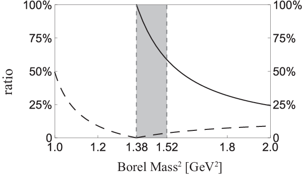
Firstly, we examine how large is the off-diagonal term $\Pi_{12}(M_{B}^{2})$ defined in Eq. (12). As shown in Fig. 5 using the solid curve, the ratio $\Pi_{12}^{2}/(\Pi_{11}\Pi_{22})$ is quite large, so the mixing should be taken into account. Accordingly, we diagonalize the matrix

at around $M_{B}^{2}=1.4$ GeV² and $s_{0}=7.6$ GeV² (we shall see that these two values are both inside the working regions for the mixed current $J_{2}$). We obtain two new currents with the mixing angle $\theta=16.3^{\rm o}$:

As shown in Fig. 5 using the dashed curve, the new ratio $(\Pi_{J_{1}J_{2}})^{2}/(\Pi_{J_{1}J_{1}}\Pi_{J_{2}J_{2}})$ is significantly suppressed in the region $1.38$ GeV${}^{2}<M_{B}^{2}<1.52$ GeV² (Borel window for $J_{2}$ when setting $s_{0}=7.6$ GeV²), so $J_{1}$ and $J_{2}$ only weakly correlate with each other inside this region.

We separately use $J_{1}$ and $J_{2}$ to perform QCD sum rule analyses. When using $J_{1}$, we find that there exist non-vanishing Borel windows as long as $s_{0}\geq 9.4$ GeV², and the mass extracted is around 3.14 GeV, even larger than 3.0 GeV, so we shall not use it to draw any conclusion.

When using $J_{2}$, we find that there exist non-vanishing Borel windows as long as $s_{0}\geq 7.2$ GeV². We show the mass extracted from $J_{2}$ in Fig. 6 as a function of the threshold value $s_{0}$ (left) and the Borel mass $M_{B}$ (right). Using the working regions $6.6$ GeV${}^{2}<s_{0}<8.6$ GeV² and $1.38$ GeV${}^{2}<M_{B}^{2}<1.52$ GeV² (Borel window for $s_{0}=7.6$ GeV²), we obtain

where the central value corresponds to $s_{0}=7.6$ GeV² and $M_{B}^{2}=1.45$ GeV². Here we have temporarily assumed the uncertainty of the mixing angle to be $\theta=16.3^{\rm o}\pm 10.0^{\rm o}$, since $J_{1}$ and $J_{2}$ become correlated again when $\theta$ is outside this region. The mass uncertainty due to this angle is $2.51^{+0.04}_{-0.03}$ GeV, that is not so large.

In this paper we use the method of QCD sum rules to study the $ss\bar{s}\bar{s}$ tetraquark states of $J^{PC}=0^{-+}$. We systematically construct all the relevant diquark-antidiquark $(ss)(\bar{s}\bar{s})$ and meson-meson $(\bar{s}s)(\bar{s}s)$ interpolating currents, and derive their relations through the Fierz transformation. We find two independent currents $\eta_{1}$ and $\eta_{2}$, and calculate both their diagonal and off-diagonal two-point correlation functions. The obtained results suggest that these two single currents strongly correlate with each other. Hence, we use them to further construct two mixed currents $J_{1}$ and $J_{2}$, which only weakly correlate with each other.

We use the two single currents $\eta_{1}$ and $\eta_{2}$ as well as the two mixed currents $J_{1}$ and $J_{2}$ to perform QCD sum rule analyses. We find the correlation functions $\Pi_{11}(M_{B}^{2})$ and $\Pi_{22}(M_{B}^{2})$ to be both negative in the region $s_{0}<4.0$ GeV² when taking $M_{B}^{2}=1.5$ GeV². This suggests that these currents couple weakly to the lower state $\eta(1475)$ as well as the $\eta^{\prime}f_{0}(980)$ threshold, so the state they couple to, as if they can couple to some state, should be new and possibly exotic.

After performing numerical analyses, we extract the masses from $\eta_{1}$ and $\eta_{2}$ to be $2.86^{+0.18}_{-0.12}$ GeV and $2.59^{+0.14}_{-0.10}$ GeV respectively, and the masses from $J_{1}$ and $J_{2}$ to be around 3.14 GeV and $2.51^{+0.14}_{-0.12}$ GeV respectively. These mass values are not affected much by the lower state $\eta(1475)$ as well as the $\eta^{\prime}f_{0}(980)$ threshold, because the currents couple weakly to them. However, there may exist some other thresholds, which are difficult to be fully taken into account.

Especially, the mass extracted from the mixed current $J_{2}$ is the lowest:

Use the Fierz transformation given in Eqs. (10), we can transform $J_{2}$ to be

This suggests that the state $X$, coupled by this current, can decay into the following channels:

• •

  It can decay into the $\eta^{\prime}f_{0}(980)$ channel, due to the $(\bar{s}_{a}s_{a})(\bar{s}_{b}\gamma_{5}s_{b})$ operator Chen:2019wjd; Cheng:2005nb:

  	$\displaystyle\langle 0|\bar{s}_{a}s_{a}|f_{0}(980)\rangle$	$\displaystyle=$	$\displaystyle f_{f_{0}(980)}m_{f_{0}(980)}\,,$		(37)
  	$\displaystyle\langle 0|\bar{s}_{b}i\gamma_{5}s_{b}|\eta^{\prime}\rangle$	$\displaystyle=$	$\displaystyle\lambda_{\eta^{\prime}}\,,$		(38)

  where $f_{f_{0}(980)}$ and $\lambda_{\eta^{\prime}}$ are decay constants. Considering that the $f_{0}(980)$ resonance can further decay into the $\pi\pi$ and $K\bar{K}$ final states, we use the BaBar measurement Aubert:2006nu:

  $${\mathcal{B}({f_{0}(980)\to K^{+}K^{-}})\over\mathcal{B}({f_{0}(980)\to\pi^{+}\pi^{-}})}=0.69\pm 0.32\,,$$

  (39)

  to further estimate and obtain

  $${\mathcal{B}({X\to\eta^{\prime}f_{0}(980)\to\eta^{\prime}K\bar{K}})\over\mathcal{B}({X\to\eta^{\prime}f_{0}(980)\to\eta^{\prime}\pi\pi})}=0.92\pm 0.43\,.$$

  (40)

• •

  It can also decay into the $\phi\phi$ final state, due to the $(\bar{s}_{a}\sigma_{\mu\nu}s_{a})(\bar{s}_{b}\sigma^{\mu\nu}\gamma_{5}s_{b})$ operator:

  	$\displaystyle\langle 0|\bar{s}_{a}\sigma_{\mu\nu}s_{a}|\phi(p,\epsilon)\rangle$	$\displaystyle=$	$\displaystyle if_{\phi}^{T}(p_{\mu}\epsilon_{\nu}-p_{\nu}\epsilon_{\mu})\,,$		(41)
  	$\displaystyle\langle 0|\bar{s}_{a}\sigma_{\mu\nu}\gamma_{5}s_{a}|\phi(p,\epsilon)\rangle$	$\displaystyle=$	$\displaystyle-f_{\phi}^{T}\epsilon_{\mu\nu\rho\sigma}p^{\rho}\epsilon^{\sigma}\,,$		(42)

  where $f_{\phi}^{T}$ is the decay constant.

In the three BESIII experiments Ablikim:2010au; Ablikim:2019zyw; Ablikim:2016hlu, the $X(2370)$ was observed in both the $\eta^{\prime}\pi\pi$ and $\eta^{\prime}K\bar{K}$ final states, and the $X(2500)$ was observed in the $\phi\phi$ final state, indicating that both of them contain many $strangeness$ components. Accordingly, our results suggest that the $X(2500)$ can be well explained as the $ss\bar{s}\bar{s}$ tetraquark state of $J^{PC}=0^{-+}$, and the $X(2370)$ may also be explained as such a state (they might even be the same state, so that its mass spectrum and decay properties can both be well explained). To verify the above interpretation, we propose the BESIII Collaboration to further study the $\pi\pi$ and $K\bar{K}$ invariant mass spectra of the $J/\psi\to\gamma\pi\pi\eta^{\prime}$ and $J/\psi\to\gamma K\bar{K}\eta^{\prime}$ decays to examine whether there exists the $f_{0}(980)$ resonance.

We thank Cheng-Ping Shen for useful discussions. This project is supported by the National Natural Science Foundation of China under Grant No. 11722540 and the Fundamental Research Funds for the Central Universities.

References

- (1) C. Patrignani et al. [Particle Data Group], Review of Particle Physics, Chin. Phys. C 40, 100001 (2016).
- (2) Y. R. Liu, H. X. Chen, W. Chen, X. Liu and S. L. Zhu, Pentaquark and Tetraquark States, Prog. Part. Nucl. Phys. 107, 237 (2019).
- (3) R. F. Lebed, R. E. Mitchell and E. S. Swanson, Heavy-quark QCD exotica, Prog. Part. Nucl. Phys. 93, 143 (2017).
- (4) A. Esposito, A. Pilloni and A. D. Polosa, Multiquark resonances, Phys. Rept. 668, 1 (2017).
- (5) F. K. Guo, C. Hanhart, U. G. Meißner, Q. Wang, Q. Zhao, and B. S. Zou, Hadronic molecules, Rev. Mod. Phys. 90, 015004 (2018).
- (6) A. Ali, J. S. Lange and S. Stone, Exotics: Heavy pentaquarks and tetraquarks, Prog. Part. Nucl. Phys. 97, 123 (2017).
- (7) S. L. Olsen, T. Skwarnicki, and D. Zieminska, Nonstandard heavy mesons and baryons: Experimental evidence, Rev. Mod. Phys. 90, 015003 (2018).
- (8) M. Karliner, J. L. Rosner and T. Skwarnicki, Multiquark States, Ann. Rev. Nucl. Part. Sci. 68, 17 (2018).
- (9) N. Brambilla, S. Eidelman, C. Hanhart, A. Nefediev, C. P. Shen, C. E. Thomas, A. Vairo and C. Z. Yuan, The states: experimental and theoretical status and perspectives, arXiv:1907.07583 [hep-ex].
- (10) F. K. Guo, X. H. Liu and S. Sakai, Threshold cusps and triangle singularities in hadronic reactions, arXiv:1912.07030 [hep-ph].
- (11) M. Ablikim et al. [BESIII Collaboration], Confirmation of the and observation of the resonances and in , Phys. Rev. Lett. 106, 072002 (2011).
- (12) J. Z. Bai et al. [BES Collaboration], Observation of a near threshold enhancement in th p anti-p mass spectrum from radiative J / psi —¿ gamma p anti-p decays, Phys. Rev. Lett. 91, 022001 (2003).
- (13) M. Ablikim et al. [BES Collaboration], Observation of a resonance in , Phys. Rev. Lett. 95, 262001 (2005).
- (14) M. Ablikim et al. [BESIII Collaboration], Observation of a mass threshoud enhancement in decay, Chin. Phys. C 34, 421.
- (15) M. Ablikim et al. [BESIII Collaboration], Observation of the and Search for the in , arXiv:1912.11253 [hep-ex].
- (16) M. Ablikim et al. [BESIII Collaboration], Observation of pseudoscalar and tensor resonances in , Phys. Rev. D 93, 112011 (2016).
- (17) M. Ablikim et al., Observation of a resonant structure in , arXiv:2001.04131 [hep-ex].
- (18) E. Kou et al. [Belle-II Collaboration], The Belle II Physics Book, PTEP 2019, 123C01 (2019).
- (19) A. Austregesilo [GlueX Collaboration], Light-Meson Spectroscopy at GlueX, Int. J. Mod. Phys. Conf. Ser. 46, 1860029 (2018).
- (20) H. X. Chen, X. Liu, A. Hosaka and S. L. Zhu, The Y(2175) State in the QCD Sum Rule, Phys. Rev. D 78, 034012 (2008).
- (21) H. X. Chen, C. P. Shen and S. L. Zhu, A possible partner state of the , Phys. Rev. D 98, 014011 (2018).
- (22) E. L. Cui, H. M. Yang, H. X. Chen, W. Chen and C. P. Shen, QCD sum rule studies of tetraquark states with , Eur. Phys. J. C 79, 232 (2019).
- (23) J. F. Liu et al. [BES Collaboration], and the New Resonances and Observed by the BES Collaboration, Phys. Rev. D 82, 074026 (2010).
- (24) W. Qin, Q. Zhao and X. H. Zhong, Revisiting the pseudoscalar meson and glueball mixing and key issues in the search for a pseudoscalar glueball state, Phys. Rev. D 97, 096002 (2018).
- (25) J. S. Yu, Z. F. Sun, X. Liu and Q. Zhao, Categorizing resonances X(1835), X(2120) and X(2370) in the pseudoscalar meson family, Phys. Rev. D 83, 114007 (2011).
- (26) C. Deng, J. Ping, Y. Yang and F. Wang, X(1835), X(2120) and X(2370) in a flux tube model, Phys. Rev. D 86, 014008 (2012).
- (27) W. I. Eshraim, S. Janowski, F. Giacosa and D. H. Rischke, Decay of the pseudoscalar glueball into scalar and pseudoscalar mesons, Phys. Rev. D 87, 054036 (2013).
- (28) L. C. Gui, J. M. Dong, Y. Chen and Y. B. Yang, Study of the pseudoscalar glueball in radiative decays, Phys. Rev. D 100, 054511 (2019).
- (29) T. T. Pan, Q. F. L¨¹, E. Wang and D. M. Li, Strong decays of the newly observed by the BESIII Collaboration, Phys. Rev. D 94, 054030 (2016).
- (30) S. C. Xue, G. Y. Wang, G. N. Li, E. Wang and D. M. Li, The possible members of the meson nonet, Eur. Phys. J. C 78, 479 (2018).
- (31) L. M. Wang, S. Q. Luo, Z. F. Sun and X. Liu, Constructing new pseudoscalar meson nonets with the observed , , and , Phys. Rev. D 96, 034013 (2017).
- (32) C. J. Morningstar and M. J. Peardon, The Glueball spectrum from an anisotropic lattice study, Phys. Rev. D 60, 034509 (1999).
- (33) Y. Chen et al., Glueball spectrum and matrix elements on anisotropic lattices, Phys. Rev. D 73, 014516 (2006).
- (34) C. M. Richards et al. [UKQCD Collaboration], Glueball mass measurements from improved staggered fermion simulations, Phys. Rev. D 82, 034501 (2010).
- (35) E. Gregory, A. Irving, B. Lucini, C. McNeile, A. Rago, C. Richards and E. Rinaldi, Towards the glueball spectrum from unquenched lattice QCD, JHEP 1210, 170 (2012).
- (36) W. I. Eshraim and S. Schramm, Decay modes of the excited pseudoscalar glueball, Phys. Rev. D 95, 014028 (2017).
- (37) W. I. Eshraim, Decay of the pseudoscalar glueball and its first excited state into scalar and pseudoscalar mesons and their first excited states, Phys. Rev. D 100, 096007 (2019).
- (38) M. Napsuciale, E. Oset, K. Sasaki and C. A. Vaquera-Araujo, Phys. Rev. D 76, 074012 (2007).
- (39) A. Martinez Torres, K. P. Khemchandani, L. S. Geng, M. Napsuciale and E. Oset, Phys. Rev. D 78, 074031 (2008).
- (40) W. Liang, C. W. Xiao and E. Oset, Study of and with the fixed center approximation to Faddeev equations, Phys. Rev. D 88, 114024 (2013).
- (41) A. A. Kozhevnikov, Dynamical analysis of the resonance contributions to the decay , Phys. Rev. D 99, 014019 (2019).
- (42) P. Lebiedowicz, O. Nachtmann and A. Szczurek, Central exclusive diffractive production of via the intermediate state in proton-proton, Phys. Rev. D 99, 094034 (2019).
- (43) A. A. Kozhevnikov, The decay : Spin dependence of amplitude and angular distributions of photons with linear polarizations, Eur. Phys. J. A 55, 155 (2019).
- (44) M. A. Shifman, A. I. Vainshtein and V. I. Zakharov, QCD And Resonance Physics. Sum Rules, Nucl. Phys. B 147, 385 (1979).
- (45) L. J. Reinders, H. Rubinstein and S. Yazaki, Hadron Properties From QCD Sum Rules, Phys. Rept. 127, 1 (1985).
- (46) K. C. Yang, W. Y. P. Hwang, E. M. Henley and L. S. Kisslinger, QCD sum rules and neutron proton mass difference, Phys. Rev. D 47, 3001 (1993).
- (47) S. Narison, QCD as a theory of hadrons (from partons to confinement), Camb. Monogr. Part. Phys. Nucl. Phys. Cosmol. 17, 1 (2002).
- (48) V. Gimenez, V. Lubicz, F. Mescia, V. Porretti and J. Reyes, Operator product expansion and quark condensate from lattice QCD in coordinate space, Eur. Phys. J. C 41, 535 (2005).
- (49) M. Jamin, Flavour-symmetry breaking of the quark condensate and chiral corrections to the Gell-Mann-Oakes-Renner relation, Phys. Lett. B 538, 71 (2002).
- (50) B. L. Ioffe and K. N. Zyablyuk, Gluon condensate in charmonium sum rules with 3-loop corrections, Eur. Phys. J. C 27, 229 (2003).
- (51) A. A. Ovchinnikov and A. A. Pivovarov, QCD Sum Rule Calculation Of The Quark Gluon Condensate, Sov. J. Nucl. Phys. 48, 721 (1988) [Yad. Fiz. 48, 1135 (1988)].
- (52) J. R. Ellis, E. Gardi, M. Karliner and M. A. Samuel, Renormalization-scheme dependence of Pade summation in QCD, Phys. Rev. D 54, 6986 (1996).
- (53) H. Y. Cheng, C. K. Chua and K. C. Yang, Charmless hadronic B decays involving scalar mesons: Implications to the nature of light scalar mesons, Phys. Rev. D 73, 014017 (2006).
- (54) H. X. Chen, Decay properties of the through the Fierz rearrangement, arXiv:1910.03269 [hep-ph].
- (55) B. Aubert et al. [BaBar Collaboration], Dalitz plot analysis of the decay , Phys. Rev. D 74, 032003 (2006).