A proof of Hall’s conjecture on length of ray images under starlike mappings of order Thanks: File: PeterSamy˙Hall˙final.tex, printed: 11-8-2026, 18.41
Abstract.
Assume that lies in the class of starlike functions of order , that is, which are regular and univalent for and such that
In this paper we show that for each , the following sharp inequality holds:
This settles the conjecture of Hall (1980) positively.
Key words and phrases:
Ray-image, length of ray-image, starlike and univalent mappings, starlike functions of order .2000 Mathematics Subject Classification
Primary 30C45, 30C20; Secondary 30C351. Introduction and the Main Theorem
The theory of univalent functions on domains in the complex plane attracted the attention of many for more than a century, and it has been centered around the class of functions regular and univalent in the unit disk and normalized by the condition The conjecture of Bieberbach which asserted for all (if ), was solved by de Branges [6] in 1984. The family together with some of its geometric subfamilies play a key role in solving many extremal problems, and a large amount of research has been done as evidenced by the volume of articles in the literature (cf. [10, 13, 14, 18, 24, 28]) and several monographs (cf. [15, 23, 25]). It is still an active field of research in view of several open problems and extensions in several settings [1, 19], including planar harmonic univalent mappings [9, 11].
This article concerns length of ray images under a special class of conformal mappings. Suppose that and maps onto a domain . Let denote the image in of the ray joining to under the mapping belonging to the family . Then the length of the curve is given by
In 1963, Gehring and Hayman [12] showed that if , i.e. is starlike (with respect to the origin), then there exists an absolute constant such that
| (1) |
We refer to this as Gehring–Hayman inequality. Motivated by this remarkable fact, Sheil-Small [29] showed that if , then the constant in (1) can be chosen to be , and if (see equation (2)), then the constant may be reduced to . Further investigation in this topic led Sheil-Small [29] to conjecture that if , i.e is convex, then the correct constant is . Hall [16, 17] showed that the best possible constants are and for the families and , respectively. This settled both the conjectures of Sheil-Small. See [3] for a simpler proof of Gehring–Hayman inequality (1) with for the case of univalent starlike functions. At this point it is worth recalling the fact that a function belonging to may not be convex univalent in for any . It is natural to ask for the corresponding optimal constant in (1) for several other choices of the family .
In this article, we consider a problem posed by Hall [17]. More precisely, Hall in this paper related the following:
At the Durham Symposium on Analytic Number Theory (July 1979) Professor Hayman asked in conversation what would be the sharp bound for the class of functions starlike of order , that is, which are regular and univalent for and such that
(2) I proved in [16] that in the starlike case, that is when , this bound is (sharp for the Koebe function) and it is likely that for the sharp constant is
From my result for , the upper bound can be derived: this is not sharp but numerically it is pretty good, for example for it gives .
In view of the higher difficulty level of the problem, determining the optimal constant in (1) for other choices of the family is difficult and results of this type were not available for many standard geometric subclasses of the univalent family .
In the present paper we prove the above conjecture of Hall in full generality for the class of functions starlike of order , . It is worth pointing out that the present method of proof provides also alternate proofs of the two cases, and , originally settled by Hall [16, 17].
Theorem 1.
Suppose that , i.e. is a starlike of order in the unit disk . Then
| (3) |
where and
| (4) |
Furthermore, the constant is optimal.
We refer to [2, 20] for some additional research related to Hall’s work and conjectures on optimal constants in the Gehring–Hayman inequality. Related to this problem, we remark that an attempt has been made by Chen and Ponnusamy [8] for sense-preserving univalent and -quasiconformal harmonic mappings. In order to make a statement about what this means, we need to introduce some basic notations.
Let be a complex-valued -function defined on and let be the length of the curve , where is a radial line segment from to , is fixed and . Then (cf. [7])
In [22], Keogh showed that if is a bounded, analytic and univalent function in , then, for each ,
| (5) |
where for , and the exponent in cannot be decreased. Kennedy [21] showed by examples that
is false in general for every positive function in satisfying as . In [5], Carroll and Twomey proved this result without the boundedness condition in the following form.
Theorem A. Suppose that is univalent in . Then, for any fixed , there is a constant such that
| (6) |
If, further, as then (5) holds.
Later, Beardon and Carne [4] gave a relatively simple argument to Theorem A in hyperbolic geometry and provided further examples. Thus, the two works of Hall mentioned in the introduction are sharper versions of this in the case of functions whose range is either a starlike domain or a convex domain. In spite of the higher level of difficulty, ideas of [5, 4] were considered for the class of sense-preserving planar harmonic univalent mappings in , with the normalization and (see [9, 10]). The family together with few geometric subclasses were investigated in [9, 30]. For further details, we refer to [10, 26]. If the co-analytic part is identically zero in the representation , then the class coincides with the family . Motivated by the above consideration, in 2019, Chen and Ponnusamy [8] obtained the following result for the case of planar harmonic mappings.
Theorem B. For , let be a -quasiconformal harmonic mapping. Then, for any fixed , there is a constant such that
If, further, as then
and the exponent in defined above cannot be replaced by a smaller number.
First we remark that Theorem B implies Theorem A when . Secondly, the proof of Theorem B is relatively harder than the proof of Theorem A because of the fact that the arguments of Beardon and Carne [4] for Theorem A are not applicable in the proof of Theorem B.
2. Proof of Theorem 1
2.1. Part 1: Proof of the main Theorem
Lemma 1.
Proof.
The family is rotationally invariant in the sense that belongs to whenever . Therefore, without loss of generality, let us suppose that in (3). As a consequence, we let , . Then is regular and univalent for , and . Therefore to prove (3) we have to show equivalently that
| (9) |
where is defined by (4). It remains to show that (9) holds whenever (7) holds.
Now, we let . Then, we have
Using the Herglotz representation theorem for regular functions with positive real part (cf. [14, 24, 28]) and the fact that , we also have, for ,
| (10) |
where is an increasing function for which satisfies . Therefore, using standard arguments and some computations, we find that
and
| (11) |
where . Note that , and is increasing on and so is nonnegative and has a total mass . Using (10) it follows that
| (12) |
Next we note from the definition of that
| (13) |
Regarding the first integral on the right, we find by (11) that
| (14) |
We then estimate the second of the integrals in (13). From (11) we also have
Applying Jensen’s inequality [31, p. 24] and performing exponentiation on both sides of the last relation, we get
| (15) |
Therefore, from (12) and (15) we deduce that
| (16) |
where is given by (1).
2.2. Part 2: Proof of the Inequality (7)
To establish the inequality (7), we need to evaluate the integrals and , where is defined by (1). In order to do this, we rewrite (1) in the following form
| (18) |
where
and
In order to prove the inequality (7), we need to establish several lemmas.
Let us denote , and so that and . Then (18) can be written in terms of and , which we denote by for obvious reason, and thus, we have
Our first aim is to give an upper bound for the sum in terms of a simpler integrand. We begin by giving the bound for the first term in the square bracket factor in the integrand of .
Lemma 2.
For , and ,
| (19) |
Proof.
The claim is clear if , so we assume that . As
we calculate
Subtracting this from the inequality in the statement of the lemma, we see that the claim (19) is equivalent to
or, multiplied by ,
| (20) |
When , the left-hand side of (20) is non-positive, so the claim is clear, and therefore, we may assume that and denote , where . When , both sides equal , so the inequality holds. We may next rewrite (20) equivalently as , where
We observed that and thus it suffices to show that is increasing on . We calculate
and it is non-negative when
Because , the last inequality holds if
Squaring both sides gives the equivalent condition
which holds since and . Thus, and the proof of the lemma is complete. ∎
Lemma 3.
Let , . Then with and defined as above, we have
where .
Proof.
By Lemma 2, we recall that
For the numerator of the integrand of with the change of variables as in the beginning of Subsection 2.2, i.e. precisely the second term of the square-bracked term in the expression of , we use
so that
Using these relations, we can therefore estimate
Thus, we have established the inequality
and for , it follows similarly that
Let us continue with the change of variables
Then
so that
From the relation , or equivalently the quadratic equation
we solve for with the restriction :
so that
Therefore, we conclude that
where . Interchanging the role of and in the above proof gives an analogous inequality for :
Note that . Finally, adding these two estimates, we obtain the desired claim. ∎
Let us next consider the expression in the case . Based on previous research, it is already known that the expression in Lemma 3 is maximized when . However, we will need the monotonicity, which is a stronger claim.
Lemma 4.
The function
| (21) |
is increasing in .
Proof.
It turns out that we can explicitly calculate the integrals involved in the expression. Since
we calculate
Similarly,
The other two integrals are more complicated, but we find that
When we use the formula for the term with , the number inside the arctangent is imaginary, so we use also the formula
Hence we conclude
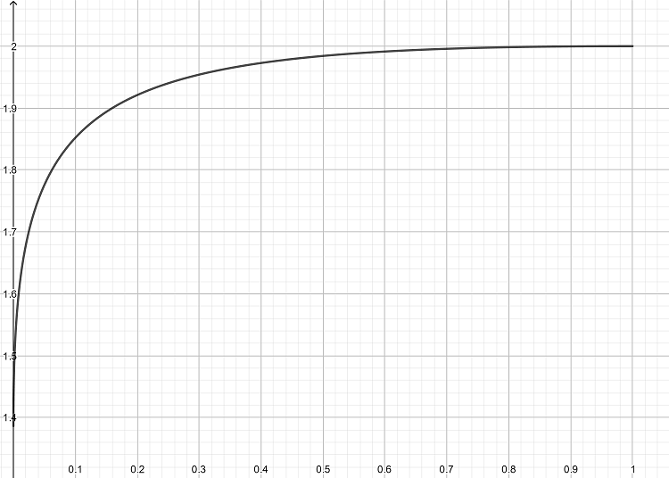
With these integral functions, we obtain that
The graph of this function, i.e. , is shown in Figure 1.
We need to show that this expression is increasing in . We change variables by defining so that and our expression equals
Since is decreasing in , we establish our claim by showing that is decreasing on . We calculate
Hence it suffices to show that
is negative. We see that , and show that is decreasing on . A calculation gives
With the new variable , we find that
We need to show that is negative on , and we observe that . To show that is decreasing on , we calculate the derivative
from which we define a function by
Finally, we observe that and
Thus for , so that is decreasing on and thus negative, which implies that is decreasing and negative for . Hence, is decreasing on , which is equivalent to the original claim. This completes the proof of the lemma. ∎
We are now ready to continue our investigation on Lemma 3, again.
Lemma 5.
Proof.
We consider the function
| (22) |
where and . We need to show that is maximized by . To that end, we consider the derivative with respect to :
In the first integral we use the change of variables and this gives
whereas in the second one we use and obtain
Therefore, we have the following expression for the derivative
Denote
and observe that the square bracket term equals . We find that
so that is increasing on and decreasing on . When , we have and so it follows that is positive until some value and then negative. Furthermore, the function
is decreasing on . Therefore, we have
both when and . We conclude that
| (23) |
Up to a constant, the right-hand side of (23) is the derivative of the function in the case . By Lemma 4, this function is increasing on , so its derivative, and hence the right-hand side of the inequality in (23) above, is non-negative. It follows that on . Furthermore, by symmetry we conclude that on . Hence the maximum of occurs at , as claimed. ∎
Finally, we are ready to prove that the inequality (7) holds when .
2.3. Proof of Theorem 1
To prove (17) it suffice to show that
Recall that and so, by Lemma 5, to suffices to show equivalently that
by the definition of . We then consider the beta function (not the function from before), and its relation to the gamma function as follows
We use this formula with and or . This gives that
since and . This completes the proof of the desired estimate (7), which, by Lemma 1 implies that the Gehring–Hayman inequality holds with constant .
It remains to be shown that given by (4) cannot be replaced by any smaller constant. We show that the extremal function for our problem is defined by . We calculate that
From this we see that . As before, we set and we have that
Furthermore, . Let us denote again . Then we have shown that
We are interested in the limit value of the right-hand side when . For some small , we restrict the integral to the range for a lower bound, and estimate
We estimate the remaining terms with the same change of variables as before:
Also as before, solving for and using (which follows from ), we have:
With the previous two estimates, we obtain
so that
The claim follows from this as .
Acknowledgements
This work was completed during the visit of the second author to the University of Turku, Finland in 2019-2020, and this author thanks Prof. Matti Vuorinen for his continuous support and his encouragement. The visit of this author was supported by a grant under “India-Finland Joint Call for Mobility of Researchers Programme” and this author acknowledges the support received from the Department of Science & Technology, Government of India, and the Academy of Finland.
Compliance with ethical standards:
Conflict of interest. The authors declare that they do not have conflict of interests.
Ethical standards. The research complies with ethical standards.
References
- [1] F. G. Avkhadiev and K.-J. Wirths, Schwarz-Pick type inequalities, Frontiers in Mathematics, Birkhäuser Verlag, Basel, 2009. viii + 156 pp.
- [2] R. Balasubramanian, V. Karunakaran and S. Ponnusamy, A proof of Hall’s conjecture on starlike mappings, J. London Math. Soc. 48(2) (1993), 271–282.
- [3] R. Balasubramanian and S. Ponnusamy, An alternate proof of Hall’s theorem on a conformal mappings inequality, Bull. Belgium Math. Soc. 3 (1996), 209–213.
- [4] A. F. Beardon and T. K. Carne, Euclidean and hyperbolic lengths of images of arcs, Proc. London Math. Soc., 97 (2008), 183–208.
- [5] T. Carroll and J. B. Twomey, Conformal mappings of close-to-convex domains, J. London Math. Soc., 55 (1997), 489–498.
- [6] L. de Branges, A proof of the Bieberbach conjecture, Acta Math. 154 (1985), 137–152.
- [7] S. L. Chen, G. Liu and S. Ponnusamy, Linear measure and -quasiconformal harmonic mappings (in Chinese), Sci. Sin. Math., 47 (2017), 1–10.
- [8] Sl. Chen and S. Ponnusamy, Radial length, radial John disks and -quasiconformal harmonic mappings, Potential Analysis 50(2019), 415–437.
- [9] J. G. Clunie and T. Sheil-Small, Harmonic univalent functions, Ann. Acad. Sci. Fenn. Ser. A. I. 9 (1984), 3–25.
- [10] P. L. Duren, Univalent Functions, Springer-Verlag, New York, (1983).
- [11] P. Duren, Harmonic mappings in the plane, Cambridge university Press, New York, (2004).
- [12] F. W. Gehring and W. K. Hayman, An inequality in the theory of conformal mapping, J. Math. Pures Appl. 41 (1963), 353–361.
- [13] G. M. Goluzin, Geometric Theory of Functions of a Complex Variable, Translations of Mathematical Monographs, Vol. 26, AMS, Providence (1969).
- [14] A. W. Goodman, Univalent Functions, Vols. I, II, Tampa, FL: Mariner (1983).
- [15] I. Graham and G. Kohr, Geometric Function Theory in One and Higher Dimensions, New York: Marcel Dekker Inc. (2003)
- [16] R. R. Hall, The length of ray-images under starlike mappings, Mathematika 23 (1976), 147–150.
- [17] R. R. Hall, A conformal mapping inequality for starlike functions of order , Bull. London Math. Soc. 12 (1980), 119–126.
- [18] W. K. Hayman, Multivalent Functions, Cambridge Tracts in Mathematics 110, 2nd ed. Cambridge: Cambridge University Press (1994).
- [19] W. K. Hayman and E. F. Lingham, Research problems in function theory, Fiftieth anniversary edition of Problem Books in Mathematics, Springer, Cham, 2019. viii+284 pp.
- [20] V. Karunakaran, Length of ray-images under conformal maps, Proc. Amer. Math. Soc. 87 (1983), 289–294.
- [21] P. B. Kennedy, Conformal mapping of bounded domains, J. London Math. Soc., 31 (1956), 332–336.
- [22] F. R. Keogh, A property of bounded schlicht functions, J. London Math. Soc., 29 (1954), 379–382.
- [23] O. Lehto, Univalent functions and Teichmüller spaces, Graduate Texts in Math. 109, Springer-Verlag, NewYork (1987).
- [24] Ch. Pommerenke, Univalent Functions, with a chapter on quadratic differentials by Gerd Jensen. Studia Mathematica/Mathematische Lehrbücher 15. Göttingen: Vandenhoeck and Ruprecht (1975).
- [25] Ch. Pommerenke, Boundary Behaviour of Conformal Maps, Springer, New York (1992)
- [26] S. Ponnusamy and A. Rasila, Planar harmonic and quasiregular mappings, Topics in Modern Function Theory (Editors. St. Ruscheweyh and S. Ponnusamy): Chapter in CMFT, RMS-Lecture Notes Series No. 19, 2013, pp. 267–333.
- [27] Malcolm I. S. Robertson, On the theory of univalent functions, Ann. of Math. 37(2) (1936), 3749–408.
- [28] St. Ruscheweyh, Convolutions in geometric function theory, Les Presses de l’Université de Montréal, Montréal (1982).
- [29] T. Sheil-Small, Some conformal mapping inequalities for starlike and convex functions, J. London Math. Soc. 1(2) (1969), 577–587.
- [30] T. Sheil-Small, Constants for planar harmonic mappings, J. London Math. Soc., 42 (1990), 237–248.
- [31] A. Zygmund, Trigonometric series, Cambridge Univ. Press, London and NewYork, 1968.