A Monotonic Optimization Approach for Solving Strictly Quasiconvex Multiobjective Programming Problems

Abstract.

In this article, we use the monotonic optimization approach to propose an outcome-space outer approximation by copolyblocks for solving strictly quasiconvex multiobjective programming problems and especially in the case that the objective functions are nonlinear fractional. After the algorithm is terminated, with any given tolerance, we obtain an approximation of the weakly efficient solution set, that contains the whole weakly efficient solution set of the problem. The algorithm is proved to be convergent and it is suitable to be implemented in parallel using standard convex programming tools. Some computational experiments are reported to show the accuracy and efficiency of the proposed algorithm.

Key words and phrases:

Multiobjective programming, monotonic optimization, strictly quasiconvex, outcome space, outer approximation.

1991 Mathematics Subject Classification

Primary: 90C29; Secondary: 90C26.

Tran Ngoc Thang¹¹¹footnotetext: Corresponding author: thang.tranngoc@hust.edu.vn and Dao Tuan Anh

School of Applied Mathematics and Informatics

Hanoi University of Science and Technology

No. 1 Dai Co Viet, Hai Ba Trung, Hanoi, Vietnam

1. Introduction

We consider the following strictly quasiconvex multiobjective programming problem

	$\displaystyle{\rm Vmin}\;$	$\displaystyle\;f(x)$		$(QVP)$
	s.t.	$\displaystyle\;x\in\mathcal{S},$

where the feasible solution set $\mathcal{S}\subset\mathbb{R}^{n}$ , $n\in\mathbb{N}^{*}$ is a nonempty, convex, compact set and the objective function $f:\mathbb{R}^{n}\rightarrow\mathbb{R}^{p}$ , $2\leq p\in\mathbb{N}^{*}$ is a strictly quasiconvex vector function on $\mathcal{S}$ , i.e. $f_{i},i=1,\dots,p$ are strictly quasiconvex functions on $\mathcal{S}$ . Recall that a continuous function $h:\mathcal{S}\rightarrow\mathbb{R}$ is called strictly quasiconvex if

h(x^{1})<h(x^{2})\Rightarrow h(\lambda x^{1}+(1-\lambda)x^{2})<h(x^{2}),

for every $x^{1},x^{2}\in\mathcal{S}$ and $0<\lambda<1$ (see [1], [15]). For two vectors $a,b\in\mathbb{R}^{r}$ with some integer $r\geq 2$ , we denote $a\leq b$ if $a_{i}\leq b_{i}$ for all $i=1,\dots,r$ . We also write $a<b$ when $a_{i}<b_{i}$ for all $i=1,\dots,r$ . For any $a,b\in\mathbb{R}^{r}$ with $a\leq b$ , the box $[a,b]$ is defined by the set of all $z\in\mathbb{R}^{r}$ such that $a\leq z\leq b.$ A feasible solution $\bar{x}$ is said to be an efficient solution (resp., weakly efficient solution) of ( ⁢ Q V P ) if there is no solution $x\in\mathcal{S}$ such that $f(x)\leq f(\bar{x})$ and $f(\bar{x})\not=f(x)$ (resp., $f(x)<f(\bar{x})$ ).

In practical computation, finding the exact efficient solution set of problem ( ⁢ Q V P ) is very difficult, even impossible, even when ( ⁢ Q V P ) is a linear multiobjective programming problem [5]. Therefore, different methods to approximate the efficient solution set have been increasingly concerned (see [6], [7], [8], [11], [13], [16],…). Namely, given a vector $\varepsilon\in\mathbb{R}_{+}^{p}$ , $\bar{x}$ is said to be a weakly $\varepsilon$ -efficient solution of ( ⁢ Q V P ) if there is no solution $x\in\mathcal{S}$ such that $f(\bar{x})-\varepsilon>f(x)$ . The sets of all efficient solutions, weakly efficient and weakly $\varepsilon$ -efficient solutions of ( ⁢ Q V P ) are respectively denoted by $\mathcal{S}_{E}$ and $\mathcal{S}_{WE}$ and $\mathcal{S}_{\varepsilon}$ .

Denote the positive orthant of $\mathbb{R}^{p}$ by $\mathbb{R}_{+}^{p}$ and its interior by ${\rm int}\mathbb{R}_{+}^{p}$ . Let $Q\subset\mathbb{R}^{p}$ be a nonempty set. We denote by ${\rm Min}Q,{\rm WMin}Q$ and $Q_{\varepsilon}$ the sets of nondominated points, weakly nondominated points and weakly $\varepsilon$ -nondominated points of $Q$ , respectively. Namely,

$\displaystyle{\rm Min}Q$	$\displaystyle=$	$\displaystyle\{q^{0}\in Q\mid(q^{0}-\mathbb{R}_{+}^{p})\cap Q=\{q^{0}\}\},$
$\displaystyle{\rm WMin}Q$	$\displaystyle=$	$\displaystyle\{q^{0}\in Q\mid(q^{0}-{\rm int}\mathbb{R}_{+}^{p})\cap Q=\emptyset\},$
$\displaystyle Q_{\varepsilon}$	$\displaystyle=$	$\displaystyle\{q^{0}\in Q\mid(q^{0}-\varepsilon-{\rm int}\mathbb{R}_{+}^{p})\cap Q=\emptyset\}.$

We denote $\text{$\mathcal{Y}$}:=f(\mathcal{S})=\{y\in\mathbb{R}^{p}\mid\exists x\in\mathbb{R}^{n},f(x)=y\}$ the outcome set or the value set of problem ( ⁢ Q V P ) . With above notations, the sets ${\rm Min}\mathcal{Y},{\rm WMin}\mathcal{Y}$ and $\mathcal{Y}_{\varepsilon}$ are the efficient, weakly efficient and weakly $\varepsilon$ -efficient outcome sets of ( ⁢ Q V P ) , respectively. They also are the images of $\mathcal{S}_{E},\mathcal{S}_{WE}$ and $\mathcal{S}_{\varepsilon}$ under $f$ , respectively.

Recall that a vector function $f=(f_{1},\dots,f_{p}),f_{i}:\mathcal{S}\rightarrow\mathbb{R}$ is usually said to be convex (resp., strictly quasiconvex) if the component functions $f_{i},i=1,\dots,p$ are convex (resp., strictly quasiconvex) on $\mathcal{S}$ (see [2], [14]). It is easily seen that if $f$ is convex then $f$ is strictly quasiconvex. Therefore, a convex multiobjective programming problem is just a special case of ( ⁢ Q V P ) .

As we know, there are many economic, financial or technical indicators which are presented by ratios or fractional functions. The objective functions, for instance, are maximization of output to input, return to risk, profit to cost, or the rate of growth… (see [5], [12],…). Consider two continuous functions $h,g$ on a nonempty convex set $S\subseteq\mathbb{R}^{n}.$ The fractional function $h/g$ is strictly quasiconvex if $h$ is non-negative convex and $g$ is positive concave on $S,$ or both $h$ and $g$ are affine (for more other forms of the strictly quasiconvex fractional function, see in [1]). By this assertion, we find that a multiobjective concave fractional program [5] and a multiobjective linear fractional program [3] are special cases of ( ⁢ Q V P ) .

Several authors have studied the structure of the efficient value set of ( ⁢ Q V P ) . In this case, ${\rm Min}\mathcal{Y}$ is connected (see [2], [14]) but is not closed even when $f$ is linear fractional [17]. However, the weakly efficient set ${\rm WMin}\mathcal{Y}$ is proved to be closed and connected. Therefore, we establish outcome-space algorithm for approximating the weakly efficient set ${\rm WMin}\mathcal{Y}$ instead of ${\rm Min}\mathcal{Y}$ . As usual, we consider the equivalently efficient set $\mathcal{Y}^{+}=\mathcal{Y}+\mathbb{R}_{+}^{p}$ which is full-dimensional and satisfies ${\rm WMin}\mathcal{Y}^{+}\cap\mathcal{Y}={\rm WMin}\mathcal{Y}.$ In general, $\mathcal{Y}^{+}$ is nonconvex, for example, $f(x)=\sqrt{\left|x\right|},S=[-1,1]$ , but $\mathcal{Y}^{+}$ has some nice property that it is a conormal set. By the monotonic analysis, a conormal set can be approximated by a copolyblock as closely as desired (see Section 2.2). Therefore, we propose an algorithm for outer approximating the set $\mathcal{Y}^{+}$ as well as the weakly efficient set ${\rm WMin}\mathcal{Y}^{+}.$ After the algorithm is terminated, we obtain an outer and an inner approximation set of the weakly efficient value set (this idea is also employed in several previous works, e.g., [10].) An approximation of the weakly efficient solution set is also obtained, which contains the whole weakly efficient solution set $\mathcal{S}_{WE}$ . The algorithm can be implemented by using standard convex programming tools.

In Section 2, we present theoretical bases and algorithms to generate a nondominated outcome point and a weakly efficient solution of problem $(QVP).$ In this section, we also present The cutting cones and outer approximate outcome sets to establish the outer approximation algorithm for solving $(QVP)$ in Section 3. The convergence of the algorithms are proved in Section 4, and Section 5 provides the computational experiment. Some concluding remarks are given is the last section.

2. Theoretical preliminaries

2.1. Generating a nondominated outcome point and a weakly efficient solution of $(QVP)$

Since the objective function $f$ is continuous and $\mathcal{S}$ is bounded, the outcome set $\mathcal{Y}$ is also bounded. Now we determine a box containing $\mathcal{Y}$ .

By the compactness of $\mathcal{Y}$ , for each $i=1,\dots,p,$ the problems of minimizing and maximizing $y_{i}$ on the feasible set $\mathcal{Y}$ have optimal solutions. It is easy to transform these problems into

\min\;\;\{f_{i}(x)\mid x\in\mathcal{S}\},

({\rm P}_{i}^{m})

and the problem

\max\;\;\{f_{i}(x)\mid x\in\mathcal{S}\}.

({\rm P}_{i}^{M})

To solve problem ( P i m ) , we utilize the strictly quasiconvexity of the objective function associated with the following remark.

Remark 2.1.

Any local optimal solution of a strictly quasiconvex programming problem is also a global optimal solution [15]. Therefore, the problem can be solved by using suitable algorithms for convex programming problems [4].

By Remark 2.1, problem ( P i m ) can be solved by convex programming tools. Note that ( P i M ) is a nonconvex problem. However, it is possible to find an upper bound of this problem without having to solve ( P i M ) (see [3] for details and illustration). Namely, for each $j=1,\dots,n$ , set

\alpha_{j}=\min\{x_{j}\mid x\in\mathcal{S}\}.

Let $\alpha^{0}=(\alpha_{1},\alpha_{2},\dots,\alpha_{n})$ and

U=\max\{\left\langle e,x\right\rangle\mid x\in\mathcal{S}\},

where $e$ is the vector of ones. Because $\mathcal{S}$ is a compact set, $U$ is a finite number. Notice also that convex programming tools are applicable to find $\alpha^{0}$ and $U$ . For each $j=1,2,\dots,n$ , define $\alpha^{j}=(\alpha_{1}^{j},\alpha_{2}^{j},\dots,\alpha_{n}^{j})^{T}$ by

\alpha_{k}^{j}=\begin{cases}\alpha_{k}^{0},\;&{\rm if}\ \ k\neq j\\ U-\sum_{k\not=j}\alpha_{k}^{0},\;&{\rm if}\ \ k=j.\end{cases}

Refer to caption — Figure 1. A 2D example of $\mathcal{S}$ and a simplex containing it

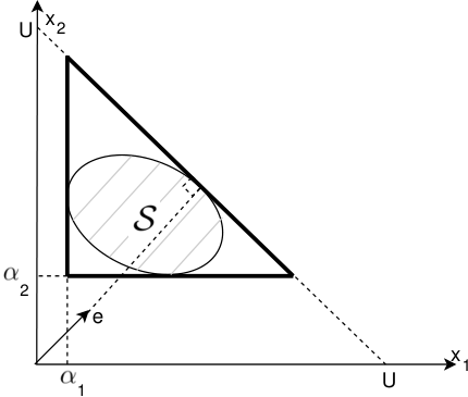
Let $\Delta$ be a simplex with the vertex set $V(\Delta)=\{\alpha^{0},\alpha^{1},\dots,\alpha^{n}\}$ . It can be verified that $\mathcal{S}\subseteq\Delta$ (see Figure 1). Therefore,

\max\{f_{i}(x)\mid x\in\mathcal{S}\}\leq\max\{f_{i}(x)\mid x\in\Delta\}.

Since $f_{i}(x),i=1,\dots,p,$ are quasiconvex and $\Delta$ is a simplex, we have

\max\{f_{i}(x)\mid x\in\Delta\}=\max\{f_{i}(x)\mid x\in V(\Delta)\}.

For each $i=1,\dots,p$ , choose a real number $M_{i}$ such that

M_{i}=\max\{f_{i}(x)\mid x\in V(\Delta)\}.

Then

M_{i}\geq\max\{f_{i}(x)\mid x\in\mathcal{S}\}.

Denote the optimal value of problem ( P i m ) by $m_{i}$ , for $i=1,\dots,p$ . Let $m=(m_{1},m_{2},\dots,m_{p})$ and $M=(M_{1},M_{2},\dots,M_{p}).$ Then we get the box $[m,M]$ such that $\mathcal{Y}\subseteq[m,M].$ The point $m$ is also known as the ideal point of the outcome set. If $m\in\mathcal{Y}$ , the set ${\rm Min}\mathcal{Y}$ consists of this point only. From now on, we assume that $m\not\in\mathcal{Y}$ .

Let

$\displaystyle\mathcal{P}^{0}$	$\displaystyle=$	$\displaystyle[m,M]=(m+\mathbb{R}_{+}^{p})\cap(M-\mathbb{R}_{+}^{p});$
$\displaystyle\mathcal{Y}^{+}$	$\displaystyle=$	$\displaystyle\mathcal{Y}+\mathbb{R}_{+}^{p};$
$\displaystyle\mathcal{Y}^{\diamond}$	$\displaystyle=$	$\displaystyle\mathcal{Y}^{+}\cap(M-\mathbb{R}_{+}^{p}).$

It is clear that $\mathcal{Y}^{+}$ and $\mathcal{Y}^{\diamond}$ have interior points and $\mathcal{Y}^{\diamond}\subset\mathcal{P}^{0}$ . The following evident properties of $\mathcal{Y}^{+}$ and $\mathcal{Y}^{\diamond}$ will be used in the sequel (see [3]).

Proposition 2.1.

We have

i) $\;{\rm Min}\mathcal{Y}={\rm Min}\mathcal{Y}^{+}={\rm Min}\mathcal{Y}^{\diamond}$ ;

ii) ${\rm WMin}\mathcal{Y}={\rm WMin}\mathcal{Y}^{+}\cap\mathcal{Y}={\rm WMin}\mathcal{Y}^{\diamond}\cap\mathcal{Y}$ .

Let $\hat{d}\in{\rm int}\mathbb{R}_{+}^{p}$ , i.e. $\hat{d}>0$ be a fixed vector and choose an arbitrary point $v\in\mathbb{R}^{p}$ . We denote $\ell(v)=\{v+t\hat{d}\mid t\in\mathbb{R}\}$ to be the line through $v$ with direction $\hat{d}$ . The intersection of $\ell(v)$ and the boundary of $\mathcal{Y}^{+}$ is determined by

w_{v}=v+t_{v}\hat{d},

(1)

where $t_{v}$ is the optimal solution of the problem

\begin{array}[]{rl}\min&t\\ {\rm s.t.}&v+t\hat{d}\in\mathcal{Y}^{+},\;t\in\mathbb{R}.\end{array}

(P^{0}(v))

The following assertion shows the way to determine a weakly nondominated outcome point.

Lemma 2.1.

Let $v$ be an arbitrary point in $\mathbb{R}^{p}$ . Then there exists the unique point $w_{v}$ determined by (1) and it is a weakly nondominated point of $\mathcal{Y}^{+}$ .

Proof.

Due to the boundedness of $\mathcal{Y}$ , given an arbitrary $v\in\mathbb{R}^{p}$ , there always exists a translation of axes so that $v$ and $\mathcal{Y}$ are two proper subsets of $\mathbb{R}_{+}^{p}$ . Hence, without loss of generality, we can make an assumption $v\cup\mathcal{Y}^{+}\subset{\rm int}\mathbb{R}_{+}^{p}$ . Under this assumption, two possible cases may occur, namely, $v\in\mathcal{Y}^{+}$ and $v\notin\mathcal{Y}^{+}$ . We investigate the lemma in each case.

Firstly, if $v\notin\mathcal{Y}^{+}$ , we denote $\ell^{+}=\{v+t\hat{d}\mid t\geq 0\}$ to be the ray starting from $v$ along direction $\hat{d}$ . As a result of [2], $\ell^{+}$ and $\partial\mathcal{Y}^{+}$ always intersect at a unique point $w_{v}\in{\rm WMin}\mathcal{Y}^{+}$ .

If $v\in\mathcal{Y}^{+}$ , because $\mathcal{Y}^{+}\in{\rm int}\mathbb{R}_{+}^{p}$ , there does not exist any line which is a subset of $\mathcal{Y}^{+}$ . Due to the closedness of $\mathcal{Y}^{+}$ , $\ell(v)\cap\mathcal{Y}^{+}$ is also closed. Let $T$ be the feasible domain of ( ⁢ P 0 ( v ) ) and $t^{*}$ its optimal solution. Due to a property of the projection $\Pi:\ell(v)\rightarrow\mathbb{R}$ , we also have that $T$ is a closed set. Obviously, if $t\in T$ and $t^{\prime}>t$ then $t^{\prime}\in T$ . By definition, $\ell^{+}=\{v+t\hat{d}\mid t\geq 0\}\in\mathcal{Y}^{+}$ . Thus, either $t^{*}=-\infty$ or $t^{*}\in T$ finite and $t^{*}\leq 0$ . If $t^{*}=-\infty$ then $\ell(v)$ is a proper subset of $\mathcal{Y}^{+}$ . This statement contradicts the fact that such line does not exist. This yields $t^{*}\leq 0$ has to be a finite real number. At that point, we let $w_{v}=v+t^{*}\hat{d}$ . It can easily be seen that $w$ belongs to the boundary of $\mathcal{Y}^{+}$ . Indeed, by definition, we already have $\bar{w}\in\mathcal{Y}^{+}$ . Moreover, for all $\delta>0$ , the ball $B_{\delta}(w)$ of radius $\delta$ centered at $w$ always contains a point $\tilde{w}=v+\tilde{t}\hat{d}\in\Gamma,\tilde{t}<t^{*}$ which does not belong to $\mathcal{Y}^{+}$ .

Assuming $w\notin{\rm WMin}\mathcal{Y}^{+}$ , then there exists a point $w^{\prime}\in(w-{\rm int}\mathbb{R}_{+}^{p})\cap\mathcal{Y}^{+}<w$ . Therefore, the ball $B_{\delta^{\prime}}(w)$ centered at $w$ of some positive radius $\delta^{\prime}$ such that $B_{\delta^{\prime}}(w)\subset w^{\prime}+{\rm int}\mathbb{R}_{+}^{p}\subset\mathcal{Y}^{+}$ exists, which contradicts $w\in\partial\text{$\mathcal{Y}$}^{+}$ . The proof is complete.∎

The explicit form of ( ⁢ P 0 ( v ) ) is the following problem

$\displaystyle\min\,\,$	$\displaystyle t$	$(P^{1}(v))$
s.t.	$\displaystyle f(x)-t\hat{d}-v\leq 0,$
	$\displaystyle x\in\mathcal{\mathcal{S}},\;t\in\mathbb{R}.$

This problem is nonconvex in general, for example, $f(x)=\sqrt{|x|},\mathcal{\mathcal{S}}=[-1,1].$ Therefore, it is difficult to determine a weakly nondominated outcome point as well as a weakly efficient solution of $(QVP)$ . However, we can transform problem ( ⁢ P 0 ( v ) ) into the form

	$\displaystyle\min\,\,$	$\displaystyle\max\{\dfrac{f_{j}(x)-v_{j}}{\hat{d}_{j}}\mid j=1,...,p\}$		$(P^{2}(v))$
	s.t.	$\displaystyle x\in\mathcal{\mathcal{S}}.$

It is worthy to note that ( ⁢ P 2 ( v ) ) can be viewed as a weighted Chebyshev function (see [9]) of which weights are $\frac{1}{\hat{d}_{j}}$ . The following lemma shows that ( ⁢ P 2 ( v ) ) is equivalent to ( ⁢ P 0 ( v ) ) and it is a problem of minimizing a strictly quasiconvex function over a convex set.

Lemma 2.2.

Problems ( ⁢ P 0 ( v ) ) and ( ⁢ P 2 ( v ) ) are equivalent, i.e. if $(x^{*},t^{*})$ is the optimal solution of ( ⁢ P 0 ( v ) ) then $x^{*}$ is the optimal solution of ( ⁢ P 2 ( v ) ) ; conversely, if $x^{*}$ is the optimal solution and $t^{*}$ is the optimal value of problem ( ⁢ P 2 ( v ) ) then $(x^{*},t^{*})$ is the optimal solution of ( ⁢ P 0 ( v ) ) . Moreover, problem ( ⁢ P 2 ( v ) ) is a strictly quasiconvex programming problem.

Proof.

We consider this proof under the known equivalence of ( ⁢ P 0 ( v ) ) and ( ⁢ P 1 ( v ) ) . Let $(x^{*},t^{*})$ be the optimal solution of ( ⁢ P 1 ( v ) ) . The feasible condition of ( ⁢ P 1 ( v ) ) can be rewritten as

t\geq\max\{\dfrac{f_{j}(x)-v_{j}}{\hat{d}_{j}}\mid j=1,\dots,p\},\;x\in\mathcal{S},\;t\in\mathbb{R}.

Assuming there exists $x\in\mathcal{S}$ such that

\max\{\dfrac{f_{j}(x)-v_{j}}{\hat{d}_{j}}\mid j=1,\dots,p\}<\max\{\dfrac{f_{j}(x^{*})-v_{j}}{\hat{d}_{j}}\mid j=1,\dots,p\}.

Let $t=\max\{\dfrac{f_{j}(x)-v_{j}}{\hat{d}_{j}}\mid j=1,\dots,p\}$ then $(x,t)$ is feasible and corresponds to a better objective value of ( ⁢ P 1 ( v ) ) , which is contrary. Therefore,

x^{*}=\min\{\max\{\dfrac{f_{j}(x)-v_{j}}{\hat{d}_{j}}\mid j=1,\dots,p\},x\in S\}.

This is sufficient to conclude that $x^{*}$ is the optimal solution of ( ⁢ P 2 ( v ) ) .

On the other hand, let $x^{*}$ be the optimal solution and $t^{*}$ be the optimal value of ( ⁢ P 2 ( v ) ) . We have $x^{*}\in\mathcal{S}$ and $t^{*}=\max\{\dfrac{f_{j}(x^{*})-v_{j}}{\hat{d}_{j}}\mid j=1,\dots,p\}\in\mathbb{R}$ so that $(x^{*},t^{*})$ belongs to the feasible domain of ( ⁢ P 1 ( v ) ) . We now assume there exists $x\in\mathcal{S},t\in\mathbb{R}$ such that $t<t^{*}$ and $f(x)-t\hat{d}-v\leq 0$ . This yields that $t\geq\max\{\dfrac{f_{j}(x)-v_{j}}{\hat{d}_{j}}\mid j=1,\dots,p\}$ . Therefore, the objective value of $(P^{2}(f(x)))$ is less than $t^{*}$ . This contradicts the fact that $t^{*}$ is the optimal value of ( ⁢ P 2 ( v ) ) . In other words, $(x^{*},t^{*})$ must be the optimal solution of ( ⁢ P 1 ( v ) ) .

Because each $f_{j}(x)$ is a strictly quasiconvex function and each $\hat{d}_{j}>0$ , from [15], we have that $\max\{\dfrac{f_{j}(x)-v_{j}}{\hat{d}_{j}}\},j=1,\dots,p$ are also strictly quasiconvex functions. Hence, ( ⁢ P 2 ( v ) ) is a strictly quasiconvex programming problem.∎

The next theorem is crucial for the method to generate a nondominated outcome point and a weakly efficient solution of $(QVP)$ .

Theorem 2.3.

For any point $v\in\mathbb{R}^{p}$ , let $x_{v}$ and $t_{v}$ be the optimal solution and the optimal value of the problem ( ⁢ P 2 ( v ) ) , respectively. Then, $w_{v}=v+t_{v}\hat{d}$ is a weakly nondominated point of $\mathcal{Y}^{+}$ and $x_{v}$ is a weakly efficient solution of $(QVP)$ .

Proof.

According to Lemma 2.2, $(x_{v},t_{v})$ is also the optimal solution of ( ⁢ P 0 ( v ) ) . By Lemma 2.1, we conclude that $w_{v}\in{\rm WMin}\mathcal{Y}^{+}$ . The feasible domain of ( ⁢ P 1 ( v ) ) suggests that $x_{v}$ satisfies $f(x_{v})\leq v+t_{v}\hat{d}=w_{v}$ . Thus, $f(x_{v})-{\rm int}\mathbb{R}_{+}^{p}\subseteq w_{v}-{\rm int}\mathbb{R}_{+}^{p}$ so that $(f(x_{v})-{\rm int}\mathbb{R}_{+}^{p})\cap\text{$\mathcal{Y}$}^{+}=\emptyset$ . Because $f(x_{v})\in{\rm WMin}\mathcal{Y}^{+}$ , $x_{v}$ is therefore a weakly efficient solution of the problem ( ⁢ Q V P ) .∎

Remark 2.2.

From Lemma 2.2, problem ( ⁢ P 2 ( v ) ) is a strictly quasiconvex programming problem. Therefore, by Remark 2.1, ( ⁢ P 2 ( v ) ) can be solved by using some algorithms for convex programming problems.

The following corollary presents the way to verify the weakly efficient condition of any point in the decision space.

Corollary 2.1.

The point $x^{*}\in\mathbb{R}^{n}$ is a weakly efficient solution of $(QVP)$ if and only if the problem $(P^{2}(f(x^{*}))$ has the optimal value $t^{*}=0.$

Proof.

Let $v^{*}=f(x^{*})\in\mathbb{R}^{p}$ . If $t^{*}=0$ is the optimal value of $(P^{2}(v^{*}))$ , using the equivalence in Lemma 2.2, and from Lemma 2.1, we have $w^{*}=v^{*}+t^{*}\hat{d}\equiv v^{*}=f(x^{*})\in{\rm WMin}\mathcal{Y}^{+}$ . Hence, $x^{*}\in\mathcal{S}_{WE}$ . Conversely, suppose that $x^{*}$ is a weakly efficient solution of ( ⁢ Q V P ) . Then $v^{*}=f(x^{*})\in\partial\mathcal{Y}^{+}$ . It is obvious that for $t<0$ we have $v^{*}+t\hat{d}\notin\text{$\mathcal{Y}$}^{+}$ and $t^{*}=0$ is the smallest value of $t$ which satisfies the feasible condition of ( ⁢ P 0 ( v ) ) .∎

Procedure 1 shows the way to generate a weakly efficient solution of ( ⁢ Q V P ) from a point $v\in\mathbb{R}^{p}$ .

Input: A point

v\in\mathbb{R}^{p}

Output: A nondominated outcome point and a weakly efficient solution of ( ⁢ Q V P ) (Remark 2.2)

Solve problem

({\rm P}^{2}(v))

to find an optimal solution

(x_{v},t_{v})

Set

w_{v}\leftarrow v+t_{v}\hat{d}

(

x_{v}

is a weakly efficient solution of ( ⁢ Q V P ) and

w_{v}

is a weakly nondominated point of

\mathcal{Y}^{+}

)

Procedure 1 1 GenerateWES(v)

Due to Corollary 2.1, an arbitrary point $x\in\mathbb{R}^{n}$ can be verified to be a weakly efficient solution of ( ⁢ Q V P ) by Procedure 2.

Input: A point

x^{*}\in\mathbb{R}^{n}

Set

v\leftarrow f(x^{*})

Solve problem

({\rm P}^{2}(v))

to find an optimal solution

(x_{v},t_{v})

if $t_{v}=0$ then 1

x^{*}

is a weakly efficient solution of ( ⁢ Q V P ) end if 2

Procedure 2 2 VerifyWES(

x^{*}

)

2.2. The cutting cones and outer approximate outcome sets

For convenience, we first recall some concepts of monotonic optimization which have been developed in [18] and [19]. Consider a set $Q\subset\mathbb{R}^{p}$ contained in box $[m,M].$ The set $Q$ is called normal if $[m,y]\subset Q$ for all $y\in Q,$ and is called conormal if $[y,M]\subset Q$ for all $y\in Q.$ Throughout this paper, we only consider the concepts related to conormal sets.

It is known that the intersection of any family of conormal sets is a conormal set. The intersection of all conormal sets containing $Q$ is called the conormal hull of $Q$ and denoted by $\mathcal{N}(Q)$ . It is also the smallest conormal set containing $Q$ .

The conormal hull of a finite set $V\subset[m,M]$ is said to be copolyblock $P,$ with vertex set $V,$ i.e. $P=\bigcup_{v\in V}[v,M]$ or $P=\mathcal{N}(V).$ A vertex $v\in P$ is called proper if there is no vertex $v^{\prime}\in P$ such that $v^{\prime}\not=v$ and $v^{\prime}\leq v.$ An improper vertex of $P$ is an element of $V$ which is not a proper vertex. Obviously, a copolyblock is fully determined by its proper vertex set. It means that a copolyblock is the conormal hull of its proper vertices.

The following propositions recall some main properties of copolyblocks and will be used in the sequel.

Proposition 2.2.

(i) The intersection of finitely many copolyblocks is a copolyblock.

(ii) The minimum of an increasing function over a copolyblock is achieved at a proper vertex of this copolyblock.

(iii) Any compact conormal set is the intersection of a family of copolyblocks.

It is easily seen that the outcome set $\mathcal{\mathcal{Y}^{\diamond}}$ is a compact conormal set in the box $[m,M].$ Let a point $v\in[m,M]$ and $v\not\in\mathcal{Y}$ . Then, by Lemma 2.1, the point $w_{v}$ determined by (1) is a weakly nondominated point of $\mathcal{Y}^{\diamond}$ and $w_{v}\in\partial\mathcal{\mathcal{Y}^{\diamond}}.$ Moreover, since $\hat{d}>0,$ we have $w_{v}>v.$ By Proposition 2.3 in [20], the cone $\mathcal{C}(w_{v}):=w_{v}-\mathbb{R}_{+}^{p}$ separates $v$ strictly from $\mathcal{Y}^{\diamond}.$ We refer to the cone $\mathcal{C}(w_{v})$ as the cutting cone of $\mathcal{Y}^{\diamond}$ at $w_{v}.$

Proposition 2.3.

Let $P$ be a copolyblock in the box $[m,M]$ with proper vertex set $V$ such that $\mathcal{\mathcal{Y}^{\diamond}}\subseteq P.$ For a given $v\in[m,M]\setminus\mathcal{\mathcal{Y}^{\diamond}}$ and $w_{v}$ determined by (1), new copolyblock $P^{\prime}$ obtained by applying the cutting cone of $\mathcal{\mathcal{Y}^{\diamond}}$ at $w_{v}$ has vertex set $V^{\prime},$ where

V^{\prime}=(V\setminus\{v\})\cup\{v-(w_{i}-v_{i})e^{i}\},\quad i=1,\dots,p.

By Proposition 2.2 (iii), we can approximate any compact conormal set by a copolyblock as closely as desired, similarly to approximating a compact convex set by a polytope. Therefore, the compact conormal set $\mathcal{Y}^{\diamond}$ can be approximated by a family of copolyblocks. Specifically, a nested sequence of copolyblocks is generated that outer-approximates the outcome set $\mathcal{Y}^{\diamond},$ i.e.

\mathcal{P}^{0}\supset\mathcal{P}^{1}\supset\dots\supset\mathcal{P}^{k}\supset\mathcal{P}^{k+1}\supset\dots\supset\mathcal{Y}^{\diamond},

where the initial copolyblock $\mathcal{P}^{0}=[m,M]$ as constructed in Section 2.1. The copolyblock $P^{k+1}$ is generated from $P^{k}$ by applying the cutting cone procedure in Proposition 2.3. The copolyblocks $\mathcal{P}^{k}$ are said to be the approximate outcome sets. From these outer approximate sets, we shall establish an outer approximation algorithm for solving $(QVP).$

3. The algorithm for solving $(QVP)$

By the outcome space approach, the solution set of $(QVP)$ is achieved by determining an approximation set contained in $\mathcal{Y}_{\varepsilon}^{\diamond}$ . Firstly, we find the set of weakly nondominated points $\mathcal{Y}_{WN}$ and the set of the outer approximation vertices $V_{\varepsilon}.$ Then we can determine the inner and outer approximation set $\mathcal{L}$ and $\mathcal{U}$ of $\mathcal{Y}^{\diamond}.$

We propose an outer approximation algorithm to determine weakly nondominated points of the outcome set $\mathcal{Y}$ . Starting from the copolyblock $\mathcal{P}^{0}=[m,M],$ we iteratively construct a sequence of copolyblocks $\{\mathcal{P}^{k}\}$ such that

\mathcal{P}^{0}\supset\mathcal{P}^{1}\supset\dots\supset\mathcal{P}^{k}\supset\mathcal{P}^{k+1}\supset\dots\supset\mathcal{Y}^{\diamond}.

We will make use of the following notations:

$\Box$

$V^{k}$ is the set of all proper vertices which determines $\mathcal{P}^{k}$ ;
$\Box$

$V_{\varepsilon}$ is a collection of outer approximate weakly nondominated points;
$\Box$

$\mathcal{Y}_{WN}$ is a collection of weakly efficient values.

At the initial step with $k=0,$ we have $V^{0}=\{m\}$ , $V_{\varepsilon}=\emptyset$ and $\mathcal{Y}_{WN}=\emptyset$ .

In a typical iteration $k$ , if every vertex in $V^{k}$ is an outer approximate weakly nondominated point, the algorithm terminates. Otherwise, there is some $v^{k}\in V^{k}\setminus V_{\varepsilon}$ . In this case, by solving $({\rm P}^{2}(v^{k})),$ we find a new weakly efficient value $f(x^{k})$ of ( ⁢ Q V P ) and add it into the set $\mathcal{Y}_{WN}.$ We also obtain a weakly nondominated point $w^{k}=v^{k}+t_{k}\hat{d}$ of $\mathcal{Y}^{+}$ , where $(x^{k},t_{k})$ is the optimal solution of $({\rm P}(v^{k}))$ . If $v^{k}$ is close enough to $w^{k}$ , $v^{k}$ is an outer approximate weakly nondominated point and is added to $V_{\varepsilon}$ . Otherwise, a new approximation $\mathcal{P}^{k+1}$ is determined by applying the cutting cone procedure in Proposition 2.3. As proved later, for sufficiently large $k$ , all vertices of $\mathcal{P}^{k}$ are close enough to $\mathcal{Y}^{\diamond}$ and the algorithm terminates. This algorithm is described in Algorithm Solve(QVP) and Procedure RIV( $V^{k+1}$ , $v^{k}$ , $w^{k}$ ) as follows.

Input: The new vertex set

V^{k+1}

probably including improper elements, previously chosen

v^{k}

, corresponding weakly nondominated point

w^{k}

Output: The new vertex set

V^{k+1}

with all proper elements.

foreach $w\in V^{k}\setminus\{v^{k}\}$ do 1

if $w\geq v^{k}$ and $w_{k}<w^{k}_{i}$ for exactly one $i$ in $\{1,\dots,p\}$ then 2

/* i.e.,

\exists i

such that

w_{i}<w^{k}_{i},w_{j}\geq w^{k}_{j}\;\;\forall j\neq i,\;\;i,j\in\{1,\dots,p\}

. */

Remove

w_{i}^{k}

. end if 3

end foreach 4

Procedure RIV(

V^{k+1}

v^{k}

w^{k}

) 3

Input: Objective function

f

and constraint sets.

Output: The collection of outer approximate weakly nondominated points.

Choose a tolerance level

\varepsilon=\epsilon{e}\geq 0

where

\epsilon\in\mathbb{R}

and

e=(1,\dots,1)\in\mathbb{R}^{p}

.
Find two points

m,M

by solving the problems

(P_{i}^{m}),(P_{i}^{M})

for

i=1,\dots,p

;

\mathcal{P}^{0}\leftarrow[m,M].

Determine the set

V^{0}

and choose a direction

\hat{d}>0

, for instance

\hat{d}=e

.
Initialize

V_{\varepsilon}\leftarrow\emptyset;\;\mathcal{Y}_{WN}\leftarrow\emptyset;\;k\leftarrow 0.

while $V^{k}\setminus V_{\varepsilon}\not=\emptyset\;$ do

Choose any

v^{k}\in V^{k}\setminus V_{\varepsilon}

.
Solve problem

({\rm P}^{2}(v^{k}))

to find an optimal solution

(x^{k},t_{k})

and set

w^{k}\leftarrow v^{k}+t_{k}\hat{d}

;

\mathcal{Y}_{WN}\leftarrow\mathcal{Y}_{WN}\cup\{f(x^{k})\}

.
if $\|w^{k}-v^{k}\|\leq\epsilon$ then

V_{\varepsilon}\leftarrow V_{\varepsilon}\cup\{v^{k}\}

;
continue.
else 1

V^{k+1}\leftarrow(V^{k}\setminus\{v^{k}\})\cup\{v^{k}-(w_{i}^{k}-v_{i}^{k})e^{i}\},i=1,\dots,p

;
Remove improper elements by Procedure RIV(

V^{k+1}

v^{k}

w^{k}

). end if 2

k\leftarrow k+1

; end while 3

return $V_{\varepsilon}$ .

Algorithm Solve(QVP) 4

Suppose the algorithm is terminated at Iteration $K.$ Then, we obtain two sets $\mathcal{Y}_{WN}$ and $V_{\varepsilon}.$ From these sets, we define

\mathcal{L}:=\mathcal{N}(\mathcal{Y}_{WN})

and

\mathcal{U}:=\mathcal{N}(V_{\varepsilon})\equiv\mathcal{P}^{K}.

It can be verified that $\mathcal{L}$ and $\mathcal{U}$ are inner and outer approximation of $\mathcal{Y}^{\diamond}$ respectively, and their weakly nondominated sets are approximate weakly nondominated sets of $\mathcal{Y}^{\diamond}.$ Based on the outer approximation $\mathcal{U},$ we can establish the outer approximation $ES$ of the weakly efficient solution set $\mathcal{S}_{WE}$ of problem $(QVP),$ that is

ES:=\underset{y\in\mathcal{U}_{\varepsilon}\cap\mathcal{Y}^{\diamond}}{\bigcup}\{x\in\mathcal{S}\mid f(x)\leq y\}

By Corollary 4.7 in the following section, it is proved that $ES$ contains the weakly $\varepsilon-$ efficient solution of $(QVP)$ and also contains the whole weakly efficient solution set of this problem.

4. The convergence of Algorithm $Solve$ $(QVP)$

We will consider Hausdorff distance between two closed sets $Q_{1},Q_{2}\subset\mathbb{R}^{p}$ defined as follows.

	$\displaystyle d_{H}(Q_{1},Q_{2})$	$\displaystyle=$	$\displaystyle\mbox{inf}\{t>0:Q_{1}\subseteq Q_{2}+tU_{p},Q_{2}\subseteq Q_{1}+tU_{p}\}$
		$\displaystyle=$	$\displaystyle\mbox{max}\{\underset{v_{1}\in Q_{1}}{\mbox{sup}}d(v_{1},Q_{2}),\underset{v_{2}\in Q_{2}}{\mbox{sup}}d(v_{2},Q_{1})\},$

where $U_{p}$ is the closed unit ball in $\mathbb{R}^{p}$ and the distance from a point $v$ to a set $Q\subset\mathbb{R}^{p}$ is defined by $d(v,Q)=\underset{y\in Q}{\mbox{inf}}||v-y||$ . We say that a sequence of nonempty closed sets $\{Q_{k}\}_{k=1}^{\infty}\subseteq\mathbb{R}^{p}$ converges to a closed set $Q$ if $\mbox{lim}_{k\rightarrow\infty}d_{H}(Q_{k},Q)=0$ and write $\mbox{lim}_{k\rightarrow\infty}Q_{k}=Q$ .

Lemma 4.1.

For each $v\in\mathcal{P}^{0}\setminus\mathcal{Y}^{\diamond}$ , we have $d(v,\mathcal{Y}^{\diamond})=d(v,\mathcal{Y}^{+})$ .

Proof.

We consider the distance between a point $v\in\mathcal{P}^{0}\setminus\mathcal{Y}^{\diamond}$ and $\mathcal{Y}^{+}$

	$\displaystyle d(v,\mathcal{Y}^{+})$	$\displaystyle=$	$\displaystyle\min\{d(v,y)\mid y\in\mathcal{Y}^{+}\}$
		$\displaystyle=$	$\displaystyle\min\{d(v,y)\mid y\leq f(x),x\in\mathcal{S}\}.$

Since $\mathcal{S}$ is compact, an optimal solution of the above minimization problem always exists. In other words, the distance between $v$ and $\mathcal{Y}^{+}$ is finite, and therefore there exists a closed ball $V_{r}(v)$ of radius $r>0$ centered at $v$ satisfying

	$\displaystyle\underset{y\in\mathcal{Y}^{+}}{\min}d(v,y)$	$\displaystyle=$	$\displaystyle\underset{y\in\mathcal{Y}^{+}\cap V_{r}(v)}{\min}d(v,y)$
	$\displaystyle\Leftrightarrow d(v,\mathcal{Y}^{+})$	$\displaystyle=$	$\displaystyle d(v,\mathcal{Y}^{+}\cap V_{r}(v)).$		(2)

Let $Q$ be a compact conormal set which does not contain $v$ , and $z^{*}$ be the projection of $v$ onto $Q$ . Then, there exists a closed ball $V_{||z^{*}-v||}(v)$ centered at $v$ having $z^{*}$ a boundary point.

Suppose that $z^{*}\notin v+\mathbb{R}_{+}^{p}$ , then there exists a point $\tilde{z}\neq z^{*},\tilde{z}\notin z^{*}+\mathbb{R}_{+}^{p}$ satisfying $\tilde{z}\in\mbox{int}V_{||z^{*}-v||}(v)$ . Since $Q$ is a conormal set, $\tilde{z}\in Q$ . This contradicts the assumption of $z^{*}$ because $d(v,\tilde{z})<d(v,z^{*})$ . Thus,

z^{*}\in v+\mathbb{R}_{+}^{p}.

(3)

Now for each $y^{\prime}\in(v+\mathbb{R}_{+}^{p})\cap Q$ , let $V_{||v-y^{\prime}||}(v)$ be the closed ball centered at $v$ having a boundary point $y^{\prime}$ . Since $y^{\prime}\in v+\mathbb{R}_{+}^{P}$ , it is clear that $((y^{\prime}+\mathbb{R}_{+}^{p})\setminus y^{\prime})\cap V_{||v-y^{\prime}||}(v)=\emptyset.$ Thus, $d(v,y)>d(v,y^{\prime}),\,\forall y\in y^{\prime}+\mathbb{R}_{+}^{p}.$ Therefore, $d(v,y)$ is a continuous, increasing function of variable $y$ on $(v+\mathbb{R}_{+}^{p})\cap Q$ . From [18], its global minimum is achieved at a nondominated point of the domain. We now apply this argument twice, with $Q$ replaced by $\mathcal{Y}^{\diamond}$ and $\mathcal{Y}^{+}\cap V_{r}(v)$ . It is worth noting from Proposition 2.1 that ${\rm Min}\mathcal{Y}^{\diamond}\subseteq{\rm WMin}\mathcal{Y}^{\diamond}\cap\mathcal{Y}$ and ${\rm Min}\mathcal{Y}^{+}\subseteq{\rm WMin}\mathcal{Y}^{+}\cap\mathcal{Y}$ . Combining these facts with (2) and (3), we deduce that the projection of $v$ on $\mathcal{Y}^{\diamond}$ must be the optimal solution of $\min d(v,y)$ , subject to $y\in{\rm WMin}\mathcal{Y}^{\diamond}\cap\mathcal{Y}\cap(v+\mathbb{R}_{+}^{p})$ . Similarly, the projection of $v$ on $\mathcal{Y}^{+}$ must be the optimal solution of $\min d(v,y)$ , subject to $y\in{\rm WMin}\mathcal{Y}^{+}\cap\mathcal{Y}\cap(v+\mathbb{R}_{+}^{p})$ . It is followed by Proposition 2.1(ii) that the feasible domains of the two problems are exactly the same. The proof is complete.∎

Lemma 4.2.

At the $k^{th}$ iteration of the algorithm, let $w_{v}$ be the weakly nondominated point obtained by solving $(P^{2}(v))$ with some $v\in V^{k}$ , then

d_{H}(\mathcal{P}^{k},\mathcal{Y}^{\diamond})\leq\underset{v\in V^{k}}{\max}||w_{v}-v||.

Proof.

Since $V^{k}$ contains all vertices of $\mathcal{P}^{k}$ , it is obvious that

\max\{d(v,\mathcal{Y}^{\diamond})\mid v\in\mathcal{P}^{k}\}=\underset{z\in V^{k}}{\max}\{\max\{d(v,\mathcal{Y}^{\diamond})\mid v\in(z+\mathbb{R}_{+}^{p})\cap(M-\mathbb{R}_{+}^{p})\}\}.

Because $d(v,\mathcal{Y}^{\diamond})$ is a convex function and the box $(z+\mathbb{R}_{+}^{p})\cap(M-\mathbb{R}_{+}^{p})$ is convex,

\max\{d(v,\mathcal{Y}^{\diamond})\mid v\in(z+\mathbb{R}_{+}^{p})\cap(M-\mathbb{R}_{+}^{p})\}=d(z,\mathcal{Y}^{\diamond}).

Therefore,

d_{H}(\mathcal{P}^{k},\mathcal{Y}^{\diamond})=\underset{v\in\mathcal{P}^{k}}{\max}d(v,\mathcal{Y}^{\diamond})=\underset{v\in V^{k}}{\max}d(v,\mathcal{Y}^{\diamond}).

Since $w_{v}\in\mathcal{Y}^{+}$ for all $v\in V^{k}$ and from the result of Lemma 4.1, we have

\underset{v\in V^{k}}{\max}d(v,\mathcal{Y}^{\diamond})=\underset{v\in V^{k}}{\max}d(v,\mathcal{Y}^{+})\leq\underset{v\in V^{k}}{\max}||w_{v}-v||.

This completes the proof.∎

Lemma 4.3.

For each $v\in\mathcal{P}^{0}\setminus\mathcal{Y}^{\diamond}$ , there exists a point $M^{\prime}>M$ such that the weakly nondominated point $w_{v}$ of $\mathcal{Y}^{+}$ obtained by solving $(P^{2}(v))$ lies in box $[m,M^{\prime}]$ .

Proof.

Denote $\mathcal{N}_{d}(Q):=(Q+\mathbb{R}_{+}^{p})\cap(d-\mathbb{R}_{+}^{p})$ the conormal hull of $Q$ in the box $[m,d]$ where $Q$ is some set contained in the box $[m,M]$ . Let us rewrite ( ⁢ P 1 ( v ) ) , the equivalent problem to ( ⁢ P 2 ( v ) ) , in this form

\begin{array}[]{cc}\min&t\\ {\rm s.t.}&f(x)\in\mathcal{N}_{v+t\hat{d}}(\mathcal{Y}^{+}),\\ &x\in\mathcal{S},\;t\geq 0.\end{array}

We denote $t_{m}$ and $t_{v}$ to be the optimal values of $(P^{2}(m))$ and $(P^{2}(v))$ , respectively. The existence of these values has been proved in Lemma 2.1. Since $m<v$ for all $v\in\mathcal{P}^{0}\setminus\mathcal{Y}^{\diamond}$ , $\{(x,t)\mid f(x)\in\mathcal{N}_{m+t\hat{d}}(\mathcal{Y}^{+}),x\in\mathcal{S},t\geq 0\}$ the feasible domain of $(P^{2}(m))$ is a subset of $\{(x,t)\mid f(x)\in\mathcal{N}_{v+t\hat{d}}(\mathcal{Y}^{+}),x\in\mathcal{S},t\geq 0\}$ the feasible domain of any $v\in\mathcal{P}^{0}\setminus\mathcal{Y}^{\diamond}$ . Therefore, the relation $t_{v}\leq t_{m}$ holds for such $v$ . We can therefore write $w_{v}=v+t_{v}\hat{d}\leq v+t_{m}\hat{d}\leq M+t_{m}\hat{d}=M^{\prime}$ .

Moreover, it is obvious that $m\leq v\leq w_{v}$ , which completes the proof.∎

Lemma 4.4.

For $\varepsilon=0$ either of two following statements is true.

i) There exists a finite number $k$ such that

\underset{v\in V^{k}}{\max}||w_{v}-v||=0;

ii) The number $k$ tends to infinity and

\underset{k\rightarrow\infty}{\lim}\underset{v\in V^{k}}{\max}||w_{v}-v||=0,

where $V^{k}$ is the set of all proper vertices determining $\mathcal{P}^{k}$ and $w_{v}$ is the corresponding weakly nondominated point of $\mathcal{Y}^{+}$ obtained by solving $(P^{2}(v))$ .

Proof.

Let $\hat{\mathcal{P}}^{0}=[m,M^{\prime}],$ with $M^{\prime}=M+t_{m}\hat{d}$ . At the $k^{th}$ iteration, we can also determine a copolyblock $\hat{\mathcal{P}}^{k+1}$ in box $[m,M^{\prime}]$ along with $\mathcal{P}^{k+1}$ . It is clear that $\mathcal{P}^{k}\subseteq\hat{\mathcal{P}}^{k}$ and $\hat{\mathcal{P}}^{k+1}\subseteq\hat{\mathcal{P}}^{k}$ for any $k\geq 0$ . From Lemma 4.3, $w_{v}\in\hat{\mathcal{P}}^{k}$ , for each $v\in\mathcal{P}^{k}\setminus\mathcal{Y}^{\diamond}$ . Now consider $v^{k}\in\mathcal{P}^{k}$ chosen at the $k^{th}$ iteration and $t_{k}$ the optimal values of $(P^{2}(v^{k}))$ . As before, let $w_{v^{k}}=v^{k}+t_{k}\hat{d}$ . We have

\mbox{Vol}[v^{k},w_{v^{k}}]=(t_{k})^{p}\mbox{Vol}[0,\hat{d}].

(4)

The lemma holds if $\underset{v\in V^{k}}{\max}||w_{v}-v||=0$ at some $k\geq 0$ . Otherwise, there exists $v^{k}\in V^{k}$ such that $||w_{v^{k}}-v^{k}||=\underset{v\in V^{k}}{\max}||w_{v}-v||>0$ . We also have $\mathcal{P}^{k+1}\subseteq\mathcal{P}^{k}\setminus(v^{k}-{\rm int}\mathbb{R}_{+}^{p})$ , noting that the equality holds when no improper vertex appears during the cut. Since $[v^{k},w_{v^{k}}]\subseteq\hat{\mathcal{P}}^{k}$ followed by the definition of $w_{v^{k}}$ , the volume of $\hat{\mathcal{P}}^{k}$ satisfies

\mbox{Vol}\hat{\mathcal{P}}^{k}-\mbox{Vol}\hat{\mathcal{P}}^{k+1}\geq\mbox{Vol}[v^{k},w_{v^{k}}].

(5)

Combining (5) with (4), we obtain

\mbox{Vol}\hat{\mathcal{P}}^{k}-\mbox{Vol}\hat{\mathcal{P}}^{k+1}\geq(t_{k})^{p}\mbox{Vol}[0,\hat{d}].

Therefore,

\begin{array}[]{ccc}\sum_{i=0}^{k}(\mbox{Vol}\hat{\mathcal{P}}^{i}-\mbox{Vol}\hat{\mathcal{P}}^{i+1})&\geq&\left(\sum_{i=0}^{k}(t_{i})^{p}\right)\mbox{Vol}[0,\hat{d}]\end{array}.

We deduce

\mbox{Vol}\hat{\mathcal{P}}^{0}\geq\left(\sum_{i=0}^{k}(t_{i})^{p}\right)\mbox{Vol}[0,\hat{d}]+\mbox{Vol}\hat{\mathcal{P}}^{k+1}\geq\left(\sum_{i=0}^{k}(t_{i})^{p}\right)\mbox{Vol}[0,\hat{d}],

for all $k\geq 1$ . Thus, by letting $k\rightarrow\infty$ , the positive series $\sum_{i=0}^{\infty}(t_{i})^{p}$ is upper bounded by $\mbox{Vol}\hat{\mathcal{P}}^{0}/\mbox{Vol}[0,\hat{d}],$ and therefore converges. Since $||\hat{d}||$ is bounded, for any $i\geq 1$ , we have

\lim_{i\rightarrow\infty}\underset{v\in V^{i}}{\max}||w_{v}-v||=\lim_{i\rightarrow\infty}||w_{v^{i}}-v^{i}||=\lim_{i\rightarrow\infty}t_{i}||\hat{d}||=0.

∎

Lemma 4.5.

With any $\varepsilon\geq 0$ , the sets $\mathcal{P}^{k}$ with $k\geq 0$ satisfy $\mathcal{Y}^{\diamond}\subseteq\mathcal{P}^{k+1}\subseteq\mathcal{P}^{k}.$ Moreover, by setting $\varepsilon=0$ , we have

	$\displaystyle\mathcal{Y}^{\diamond}$	$\displaystyle=$	$\displaystyle\lim_{k\rightarrow\infty}\mathcal{P}^{k}$	$\displaystyle=$	$\displaystyle\bigcap_{k\geq 1}\mathcal{P}^{k},$		(6)
	$\displaystyle{\rm WMin}\mathcal{Y}^{\diamond}$	$\displaystyle=$	$\displaystyle\lim_{k\rightarrow\infty}{\rm WMin}\mathcal{P}^{k}.$				(6)

Proof.

The proof falls naturally into three parts. From the formulation of $\mathcal{P}^{k},k\geq 0$ , the first part of the lemma is immediate. We deduce directly from Lemma 4.2 and Lemma 4.4 that

\lim_{k\rightarrow\infty}d_{H}(\mathcal{P}^{k},\mathcal{Y}^{\diamond})\leq\lim_{k\rightarrow\infty}\max_{v\in V^{k}}||w_{v}-v||=0.

Therefore, $\{\mathcal{P}^{k}\}_{k\geq 0}$ converges to $\mathcal{Y}^{\diamond}$ when $k$ goes to infinity.

Since $\mathcal{P}^{k+1}\subseteq\mathcal{P}^{k}$ for any $k\geq 0$ , it follows easily that $\lim{}_{k\rightarrow\infty}\mathcal{P}^{k}=\bigcap_{k\geq 1}\mathcal{P}^{k}$ . What is left is to prove the second equation of (6). Let $Q$ be a copolyblock in box $[m,M]$ , and recall the notation $Q^{+}=Q+\mathbb{R}_{+}^{p}$ , we first prove

{\rm WMin}Q=\partial Q^{+}\cap(M-\mathbb{R}_{+}^{p}).

(7)

If $\bar{w}\in{\rm WMin}Q$ then of course $\bar{w}\in(M-\mathbb{R}_{+}^{P})$ . Since the cone $\bar{w}-{\rm int}\mathbb{R}_{+}^{p}\nsubseteq Q^{+}$ , it is clear that $\bar{w}\in\partial Q^{+}$ . This yields ${\rm WMin}Q\subseteq\partial Q^{+}\cap(M-\mathbb{R}_{+}^{p})$ . Conversely, if $\bar{w}\in\partial Q^{+}\cap(M-\mathbb{R}_{+}^{p})$ . By the property of a copolyblock, $\bar{w}-{\rm int}\mathbb{R}_{+}^{p}\nsubseteq Q^{+}$ . This also means that $\bar{w}$ is a weakly nondominated point of $Q^{+}$ . Because $\bar{w}<M$ , we also have $\bar{w}\in{\rm WMin}Q$ . (7) is proved.
Applying (7) on $\mathcal{Y}^{\diamond}$ gives

{\rm WMin}\mathcal{Y}^{\diamond}=\partial\mathcal{Y}^{+}\cap(M-\mathbb{R}_{+}^{p}).

(8)

Let $\partial\mathcal{P}^{k+}$ be the boundary set of $\mathcal{P}^{k+}:=\mathcal{P}^{k}+\mathbb{R}_{+}^{p}$ . We now apply (7) again, with $\mathcal{Y}^{\diamond}$ replaced by $\mathcal{P}^{k+}$ , to obtain

{\rm WMin}\mathcal{P}^{k}=\partial\mathcal{P}^{k+}\cap(M-\mathbb{R}_{+}^{p})\subseteq\mathcal{P}^{k}.

(9)

Moreover, since $\mathcal{Y}^{+}\subseteq\mathcal{P}^{k+}$ ,

d_{H}(\partial\mathcal{P}^{k+}\cap(M-\mathbb{R}_{+}^{p}),\partial\mathcal{Y}^{+}\cap(M-\mathbb{R}_{+}^{p}))

=\max\{d(v,\partial\mathcal{Y}^{+}\cap(M-\mathbb{R}_{+}^{p}))\mid v\in\partial\mathcal{P}^{k+}\cap(M-\mathbb{R}_{+}^{p})\}.

From Lemma 4.1, for each $v$ inside the box $[m,M]$ which does not belong to $\mathcal{Y}^{\diamond}$ , we have

d(v,\mathcal{Y}^{\diamond})=d(v,\mathcal{Y}^{+})=d(v,\partial\mathcal{Y}^{+})=d(v,\partial\mathcal{Y}^{+}\cap(M-\mathbb{R}_{+}^{p})).

Thus,

d_{H}(\partial\mathcal{P}^{k+}\cap(M-\mathbb{R}_{+}^{p}),\partial\mathcal{Y}^{+}\cap(M-\mathbb{R}_{+}^{p}))\leq\max_{v\in V^{k}}d(v,\mathcal{Y}^{\diamond}).

From (7), (9) and the first equation of (6), it follows that $\lim_{k\rightarrow\infty}{\rm WMin}\mathcal{P}^{k}={\rm WMin}\mathcal{Y}^{\diamond}$ which is the desired conclusion.∎

Consider the sets $\mathcal{Y}_{WN}$ and $V_{\varepsilon}$ obtained from the algorithm. Recall that $\mathcal{L}=\mathcal{N}(\mathcal{Y}_{WN})$ and $\mathcal{U}=\mathcal{N}(V_{\varepsilon}).$ The following assertion shows that these sets are the inner and outer approximate sets of $\mathcal{Y}^{\diamond},$ respectively.

Theorem 4.6.

Let $\varepsilon=\epsilon e$ , where $e$ denotes the vector of ones in $\mathbb{R}^{p}$ . We have the following properties:

i) $\mathcal{L}\subseteq\mathcal{Y}^{\diamond}\subseteq\mathcal{U}$ ;

ii) ${\rm WMin}\mathcal{Y}^{\diamond}\subseteq\mathcal{U}_{\varepsilon}\cap\mathcal{Y}^{\diamond}\subseteq\mathcal{Y}_{\varepsilon}^{\diamond}$ ;

iii) ${\rm WMin}\mathcal{L}\subseteq\mathcal{Y}_{\varepsilon}^{\diamond}$ .

Proof.

i) is straightforward.

We now prove ii). When the algorithm terminates at the $K^{th}$ iteration, with a tolerance level $\epsilon$ , $\mathcal{U}\equiv\mathcal{P}^{K}$ is close enough to $\mathcal{Y}^{\diamond}$ , namely

\mathcal{U}\subseteq\mathcal{Y}^{\diamond}+\epsilon U_{p},

where $U_{p}$ is the closed unit ball in $\mathbb{R}^{p}$ . Let $y\in{\rm WMin}\mathcal{Y}^{\diamond}$ , it is necessary to prove $y\in\mathcal{U}_{\varepsilon}$ . For this purpose, by definition of $\mathcal{U}_{\varepsilon}$ , we need to show that

[(y-\epsilon e)-\mbox{int}\mathbb{R}_{+}^{p}]\cap\mathcal{U}=\emptyset.

(10)

Indeed, since $\mathcal{U}\subseteq\mathcal{Y}^{\diamond}+\epsilon U_{p}\subseteq\mathcal{Y}^{\diamond}-\epsilon e+\mathbb{R}_{+}^{p}$ , it is sufficient to see that the two sets in the left hand side of (10) do not intersect. Moreover, if $y\in\mathcal{U}_{\varepsilon}\cap\mathcal{Y}^{\diamond}$ , obviously, (10) is now true. Because $\mathcal{Y}^{\diamond}\subseteq\mathcal{P}^{K}$ , so $[(y-\epsilon e)-\text{int}\mathbb{R}_{+}^{p}]\cap\mathcal{Y}^{\diamond}=\emptyset$ . We conclude that $y\in\mathcal{Y}_{\varepsilon}^{\diamond}$ .

The proof for iii) is similar.∎

Theorem 4.7.

Given $\epsilon>0$ and $\varepsilon=\epsilon e$ , the algorithm terminates after a finite number of iterations and generates the approximate solution set $ES$ such that $\mathcal{S}_{WE}\subseteq ES\subseteq\mathcal{S}_{\varepsilon}$ .

Proof.

Since $\epsilon>0$ , from Lemma 4.4, there exists $K>0$ such that $||w_{v}-v||\leq\epsilon$ for all $v\in V^{K}$ at which iteration the algorithm terminates. Moreover, the necessary and sufficient condition of a weakly efficient solution $x\in\mathcal{S}_{WE}$ is that there exists some $y\in{\rm WMin}\mathcal{Y}^{\diamond}$ such that $f(x)\leq y$ . Theorem 4.6(ii) enables us to write

\mathcal{S}_{WE}\subseteq\underset{y\in{\rm WMin}\mathcal{Y}^{\diamond}}{\bigcup}\{x\in\mathcal{S}\mid f(x)\leq y\}\subseteq\underset{y\in\mathcal{U}_{\varepsilon}\cap\mathcal{Y}^{\diamond}}{\bigcup}\{x\in\mathcal{S}\mid f(x)\leq y\}=ES.

Moreover, from the definition of $\mathcal{S}_{\varepsilon}$ , we have $ES\subseteq\mathcal{S}_{\varepsilon}$ , so $\mathcal{S}_{WE}\subseteq ES\subseteq\mathcal{S}_{\varepsilon}$ . This completes the proof.∎

5. Computational Experiment

This section is used to illustrate our proposed algorithm through several numerical examples. We also want to compare our results with other related works of [5]. The algorithms were implemented in parallel on Intel(R) Xeon(R) CPU E5-2630 v4 at 2.20Ghz (32 logical cores) and 128Gb RAM using Matlab 9.3 (2017b).

Example 5.1.

Consider the following linear fractional programming problem

\begin{array}[]{cccl}\mbox{Vmin}&f_{1}(x)&=&\dfrac{-x_{1}}{x_{1}+x_{2}},\\ &f_{2}(x)&=&\dfrac{3x_{1}-2x_{2}}{x_{1}-x_{2}+3}\\ \mbox{s.t.}&x_{1},x_{2}\in\mathbb{R},\\ &x_{1}-2x_{2}&\leq&2,\\ &-x_{1}-2x_{2}&\leq&-2,\\ &-x_{1}+x_{2}&\leq&1,\\ &x_{1}&\leq&6.\end{array}

Since both objectives of this problem are a ratio of two linear functions, it is clearly a multiobjective strictly quasiconvex programming problem. Thus, we can use our algorithm to solve this problem. Let us demonstrate below the detailed computation for the case $\epsilon=0.5$ .

Initialization step. We find a lower boundary $m=(-1,-1)$ by solving the convex programming problem ( P i m ) , $i=1,2$ and choose an upper boundary $M=(0,2.6)$ .

Iteration $k=0$ . The only point in $V^{0}$ is chosen $v^{0}=m=(-1,-1)$ . Solving $(P^{2}(v^{0}))$ gives $t_{0}=0.6404$ and $w^{0}=(-0.3596,-0.3596)$ . Two new proper vertices $(-0.3596,-1.000)$ and $(-1.000,-0.3596)$ are inserted to $V^{1}$ by the cutting procedure.

Iteration $k=1$ . A point $v^{1}=(-0.3596,-1.000)$ is chosen from $V^{1}\setminus V_{\varepsilon}$ . Solving $(P^{2}(v^{1}))$ gives $t_{1}=0.1626$ and $w^{1}=(-0.1970,-0.8374)$ . Since $||w^{1}-v^{1}||=0.2299<\epsilon$ , $V_{\epsilon}=V_{\epsilon}\cup\{v^{1}\}$ . We continue to the next iteration.

Iteration $k=2$ . Choose $v^{2}=(-1.0000,-0.3596)$ . Solving $(P^{2}(v^{2}))$ gives $t_{2}=0.5257,w^{2}=(-0.4743,0.1661)$ . Vertices $(-0.4743,-0.3596)$ , $(-1.0000,0.1661)$ are inserted to $V^{3}$ by the cutting procedure.

Iteration $k=3$ . Choose $v^{3}=(-0.4743,-0.3596)$ . Solving $(P^{2}(v^{3}))$ gives $t_{3}=0.1005$ and $w^{3}=(-0.3738,-0.2591)$ . Since $||w^{3}-v^{3}||=0.1421<\epsilon$ , update $V_{\epsilon}=V_{\epsilon}\cup\{v^{3}\}$ .

Iteration $k=4$ . Choose $v^{4}=(-1.0000,0.1661)$ . Solving $(P^{2}(v^{4}))$ gives $t_{4}=0.3571,w^{4}=(-0.6429,0.5232)$ . Vertices $(-0.6429,0.1661)$ , $(-1.0000,0.5232)$ are inserted to $V^{5}$ by the cutting procedure.

Iteration $k=5$ . Choose $v^{5}=(-0.6429,0.1661)$ . Solving $(P^{2}(v^{5}))$ gives $t_{5}=0.1154,w^{5}=(-0.5275,0.2815)$ . Since $||w^{5}-v^{5}||=0.1633<\epsilon$ , update $V_{\epsilon}=V_{\epsilon}\cup\{v^{5}\}$ .

Iteration $k=6$ . Choose $v^{6}=(-1.0000,0.5232)$ . Solving $(P^{2}(v^{6}))$ gives $t_{5}=0.2377,w^{5}=(-0.7623,0.7608)$ . Since $||w^{6}-v^{6}||=0.3361<\epsilon$ , update $V_{\epsilon}=V_{\epsilon}\cup\{v^{6}\}$ .

The algorithm terminates since there is no more points in $V^{k}\setminus V_{\varepsilon}$ . We obtain the sets

	$\displaystyle\mathcal{Y}_{WN}$	$\displaystyle=\{(-0.3596,-0.3596),(-0.1970,-0.8374),(-0.4743,0.1661),$
		$\displaystyle(-0.3738,-0.2591),(-0.6429,0.5232),(-0.5275,0.2815),(-0.7623,0.7608)\}$

and

V_{\epsilon}=\{(-0.3596,-1.0000),(-0.4743,-0.3596),(-0.6429,0.1661),(-1.0000,0.5232)\}.

We compute the results in other cases of $\epsilon$ and show them in Table 1, where T, V and C denote the average computation time, number of weakly efficient values (or the number of vertices in $\mathcal{L}$ ) and number of vertices of the outer approximate copolyblock, respectively. The computational result is visualized in Figure 2.

$\epsilon$	T	V	C
0.1	1.894534	35	18
0.05	2.167836	67	34
0.025	2.644173	117	59
0.0125	4.124381	231	116

Table 1. Computational results in Example 5.1

Example 5.2.

Consider the following convex fractional minimization problem

\begin{array}[]{cccc}\mbox{Vmin}&f_{1}(x)&=&\dfrac{x_{1}+1}{-x_{1}^{2}+3x_{1}-x_{2}^{2}+3x_{2}+3.50},\\ &f_{2}(x)&=&\dfrac{x_{1}^{2}-2x_{1}+x_{2}^{2}-8x_{2}+20.00}{x_{2}}\\ \mbox{s.t.}&x_{1},x_{2}\in\mathbb{R},\\ &2x_{1}+x_{2}&\leq&6,\\ &3x_{1}+x_{2}&\leq&8,\\ &x_{1}-x_{2}&\leq&1,\\ &x_{1},x_{2}&\geq&1.\end{array}

Since both $f_{1}(x)$ and $f_{2}(x)$ are convex fractions and the feasible domain of this problem is a polyhedron, the above problem is a strictly quasiconvex multiobjective programming problem.

By choosing $\epsilon=0.1,\hat{d}=(1,1)$ , the algorithm stops after 19 iterations. We obtain the $V_{\varepsilon}$ set of 10 vertices of the approximate copolyblock and the $\mathcal{Y}_{WN}$ set including 19 weakly nondominated points. The computational results with other values of $\epsilon$ are presented in Table 2 with all notations having the same meaning as in Table 1. The computational results are illustrated in Figure 3. Two green small circles in the figure are the nondominated outcome points as stated in [5] after running its algorithm twice with different initial conditions.

$\epsilon$	T	V	C
0.08	1.764705	25	13
0.04	2.156274	70	35
0.02	2.628011	110	55
0.01	3.529236	170	84

Table 2. Computational results in Example 5.2

Example 5.3.

Consider the following convex programming problem

\begin{array}[]{cccl}\mbox{Vmin}&f_{1}(x)&=&x_{1}^{2}+x_{2}^{2}+x_{3}^{2}+10x_{2}-120x_{3},\\ &f_{2}(x)&=&x_{1}^{2}+x_{2}^{2}+x_{3}^{2}+80x_{1}-448x_{2}+80x_{3},\\ &f_{3}(x)&=&x_{1}^{2}+x_{2}^{2}+x_{3}^{2}+448x_{1}+80x_{2}+80x_{3}\end{array}

\begin{array}[]{crcl}\mbox{s.t.}&x_{1}^{2}+x_{2}^{2}+x_{3}^{2}&\leq&100,\\ &0&\leq&x_{1}\leq 10,\\ &0&\leq&x_{2}\leq 10,\\ &0&\leq&x_{3}\leq 10.\end{array}

In the initial step, we obtain $m_{1}=(-1100,-4380,-4380)$ by solving convex programming problems $(P_{1}^{m}),(P_{2}^{m}),(P_{3}^{m})$ . Instead of solving $(P_{1}^{M}),(P_{2}^{M}),(P_{3}^{M})$ , we only need to find a upper boundary $\hat{y}=(473.2051,1685.6406,1685.6406)$ . Let $m=(-1110,-4390,-4390)<m_{1},M=(2000,2000,2000)>\hat{y}$ and a positive direction $\hat{d}=(0.2,1,1)>0$ .

Computational results with different values of $\epsilon$ are presented in Table 3 with the same notation meaning as in Example 5.1.

$\epsilon$	T	V	C
800	4.748950	606	1,122
400	29.800921	13,450	24,982
200	4,766.430489	1,011,221	1,907,464

Table 3. Computational results in Example 5.3

6. Conclusion

In this paper, we propose an algorithm for solving the strictly quasiconvex multiobjective programming problem ( ⁢ Q V P ) based on the monotonic approach. Firstly, we generate a weakly efficient solution of ( ⁢ Q V P ) associated with a nondominated outcome point by using strictly quasiconvex programming. Then, we apply the cutting cones in monotonic optimization to outer approximate the outcome set. From the sets of outer approximation outcome points and nondominated outcome points, we have established the inner and outer approximation set of outcome set and obtained the approximation of weakly solution set that contains the whole weakly solution set of ( ⁢ Q V P ) with any tolerance. These properties are guaranteed by the convergence theorems. We also develop a parallel version of the proposed algorithm, that is more efficient than the former. The numerical results show that the algorithm is flexible for a large class of problems and the computational time is acceptable for a feasible tolerance. In the future, the proposed algorithm can be applied for solving many problems related to the multiobjective programming problem ( ⁢ Q V P ) .

References

[1] M. Avriel, W. E. Diewert, S. Schaible and I. Zang, Generalized Concavity, New York: Plenum Press, 1988.
[2] J. Benoist, Contractibility of the efficient set in strictly quasi-concave vector maximization, J. Optim. Theory Appl., 110 (2001), 325–336.
[3] H. P. Benson, An outer approximation algorithm for generating all efficient extreme points in the outcome set of a multiple objective linear programming problem, J. Glob. Optim., 13 (1998), 1–24.
[4] H. P. Benson, On the global optimization of sums of linear fractional functions over a convex set, J. Optim. Theory Appl., 121 (2004), 19–39.
[5] H. P. Benson, A global optimization approach for generating efficient points for multiobjective concave fractional programs, J. Multi-Crit. Decis. Anal., 13 (2005), 15–28.
[6] I. Das and J. E. Dennis, Normal-boundary intersection: a new method for generating the Pareto surface in nonlinear multicriteria optimization problems, SIAM J. Optim., 8 (1998), 631–657.
[7] M. Ehrgott, L. Shao and A. Schobel, An Approximation Algorithm for Convex Multi-objective Programming Problems, J. Glob. Optim., 50 (2011), 397–416.
[8] D. Gourion and D. T. Luc, Finding efficient solutions by free disposal outer approximation, SIAM J. Optim., 20 (2010), 2939–2958.
[9] I. Kaliszewski, J. Miroforidis and D. Podkopaev, Interactive multiple criteria decision making based on preference driven evolutionary multiobjective optimization with controllable accuracy, European Journal of Operational Research, 216(1) (2012), 188–199.
[10] I. Kaliszewski and J. Miroforidis, On upper approximations of Pareto fronts, J. Glob. Optim., 72 (2018), 475–490.
[11] K. Klamroth, J. Tind and M. M. Wiecek, Unbiased approximation in multicriteria optimization, Math. Methods Oper. Res., 56 (2002), 413–457.
[12] H. Konno and M. Inori, Bond portfolio optimization by bilinear fractional programming, J. Oper. Res. Soc. Japan, 32 (1989), 143–158.
[13] A. Lohne, B. Rudloff and F. Ulus, Primal and dual approximation algorithms for convex vector optimization problems, J. Glob. Optim., 60 (2014), 713–736.
[14] D. T. Luc, Generalized Convexity in Vector Optimization, in Handbook of Generalized Convexity and Generalized Monotonicity, Springer (2005), 195–136.
[15] O. L. Mangasarian, Nonlinear Programming, New York: McGraw-Hill, 1969.
[16] S. Ruzika and M. M. Wiecek, Approximation methods in multiobjective programming, J. Optim. Theory Appl., 126 (2005), 473–501.
[17] I. M. Stancu-Minasian, Fractional Programming: Theory, Methods and Applications, Kluwer Academic Publishers, 1997.
[18] H. Tuy, Normal sets, polyblocks and monotonic optimization, Vietnam J. Math., 27 (1999), 277–300.
[19] H. Tuy, Monotonic Optimization: Problems and Solution Approaches, SIAM J. Optim., 2 (2000), 464–494.
[20] H. Tuy, F. Al-Khayyal and P. T. Thach, Monotonic Optimization: Branch and Cuts Methods, in Essays and Surveys on Global Optimization, Springer (2005), 39–78.

Received xxxx 20xx; revised xxxx 20xx.

A Monotonic Optimization Approach for Solving Strictly Quasiconvex Multiobjective Programming Problems

Abstract.

Key words and phrases:

1991 Mathematics Subject Classification

1. Introduction

2. Theoretical preliminaries

2.1. Generating a nondominated outcome point and a weakly efficient solution of (Q​V​P)(QVP)

Remark 2.1.

Proposition 2.1.

Lemma 2.1.

Proof.

Lemma 2.2.

Proof.

Theorem 2.3.

Proof.

Remark 2.2.

Corollary 2.1.

Proof.

2.2. The cutting cones and outer approximate outcome sets

Proposition 2.2.

Proposition 2.3.

3. The algorithm for solving (Q​V​P)(QVP)

4. The convergence of Algorithm S​o​l​v​eSolve(Q​V​P)(QVP)

Lemma 4.1.

Proof.

Lemma 4.2.

Proof.

Lemma 4.3.

Proof.

Lemma 4.4.

Proof.

Lemma 4.5.

Proof.

Theorem 4.6.

Proof.

Theorem 4.7.

Proof.

5. Computational Experiment

Example 5.1.

Example 5.2.

Example 5.3.

6. Conclusion

References

2.1. Generating a nondominated outcome point and a weakly efficient solution of $(QVP)$

3. The algorithm for solving $(QVP)$

4. The convergence of Algorithm $Solve$ $(QVP)$