Quantum Computing for Quantum TunnellingPreprint: IPPP/20/8

There has been increasing interest in the possibility of simulating Quantum Field Theory (QFT) on quantum computers [1], with the development of efficient algorithms to compute scattering probabilities in simple theories of scalars and fermions [2, 3, 4, 5, 6, 7, 8, 9, 10, 11, 12, 13, 14, 15, 16, 17]. In particular it is known that by latticizing field theories, quantum computers should be able to compute scattering probabilities in QFTs with a run time that is polynomial in the desired precision, and in principle to a precision that is not bounded by the limits of perturbation theory. However a particularly difficult aspect of this programme is the preparation of scattering states [4, 6, 5, 8, 9, 14, 15, 16, 17], with several works having proposed a hybrid classical/quantum approach to solving this problem [11, 17, 18, 19]. A complementary approach is to map field theory equations to discrete quantum walks [20, 21, 22, 23] which can be simulated on a universal quantum computer.

In this paper we point out that certain nonperturbative quantum processes do not suffer from this difficulty, and lend themselves much more readily to study on quantum computers in the short term. These are the tunnelling and related processes, which are of fundamental importance for the explanation of quantum mechanical and quantum field theoretical phenomena, for example transmission rates of electron microsopes, first-order phase transitions during baryogenesis, or the potential initiation of stochastic gravitational wave spectra in the early Universe and many more.

Typically in tunnelling, the system begins in a false vacuum state that is non-dynamical and virtually trivial. The initial state can be very long lived, with tunnelling to a lower “true” vacuum state taking place via non-perturbative instanton configurations. In principle in such a process, the confinement of the initial state to a false vacuum prepares the state for us, so that the analytically straighforward perturbative phenomena are paradoxically the quantum computationally more difficult ones.

As opposed to quantum computing realised by a series of discrete “gate” operations, quantum annealers [24, 25] perform continuous time quantum computations, and therefore they are well-suited to the study of tunnelling problems by direct simulation (although our discussion could ultimately be adapted to gate-model quantum computers as well) [26, 27, 28, 29, 30, 31, 32, 33, 34, 35, 36]. In particular these devices, produced by D-Wave Systems [37], can be seeded with initial conditions using the “reverse annealing” feature,[38] allowing the simulation of dynamics. In contrast with the quantum-gate devices, they are already quite large, $2048$ qubits in the current generation, with work ongoing to develop much more connected $5000$ qubit machines. Moreover they operate in a dissipative rather than fully coherent regime, which is likely to be realistic for many real theories in which there are interactions with matter. In the present context this would be relevant for studies of so-called thermal tunnelling rather than (or in addition to) quantum tunnelling. D-Wave devices have been able successfully to simulate condensed matter systems, sometimes showing advantages over classical counterparts [39, 40, 41].

The main objective of this work is to demonstrate how a field theory problem can be successfully encoded on a quantum annealing device, and to do this we will focus on the classic problem of obtaining tunnelling rates for a system stuck in a metastable minimum (a.k.a. false vacuum).

A useful potential to focus on is the following quartic one:

$$V(\phi)\,=\,\frac{\lambda}{8}(\phi^{2}-a^{2})^{2}+\frac{\epsilon}{2a}(\phi-a)\penalty\ .$$

(1)

The potential is shown in Fig.1. On the left we show the “thick-wall” regime where $\epsilon$ is large. This limit is when the barrier is close to disappearing (or has disappeared altogether) and the walls become comparable in size to the bubble itself. For numerics we choose $a=\lambda=1$ and $\epsilon=0.3$. The opposite “thin-wall” regime (for which we choose $\epsilon=0.01$) is the limit in which $\epsilon$ is small and is approximately the difference in vacuum energy density between the false and true minima.

We are interested in the situation where the system starts in the false vacuum, and our objective is to study the rate per unit volume of tunnelling out of it. The analytic calculation of this rate is a classic problem, but it is worth briefly recapping it in order to recast the result in a form that can easily be compared with the results from a quantum simulation. It proceeds as follows.

First let us remove the extraneous constant term by working with $U(\phi)\,=\,V(\phi)\,-\,V(\phi_{+}),$ which has $U(\phi_{+})=0$. Using the well-known technique of [42, 43, 44, 45], the bubble profile is given by finding a “bounce solution” to the following differential equation:

$$\frac{d^{2}\phi}{d\rho^{2}}+\frac{c}{\rho}\frac{d\phi}{d\rho}\,=\,U^{\prime}\penalty\ ,$$

(2)

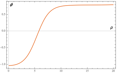
where in four dimensions, $c$ takes the value $2$ or $3$ for a finite temperature $O(3)$ symmetric bubble, or a purely quantum tunnelling $O(4)$ symmetric instanton, respectively. The required “bounce” is subject to the boundary condition that $d\phi/d\rho=0$ as $\rho\rightarrow 0,\infty$, which determines the starting value $\phi(0)$, which is the field-value at the centre of the radially symmetric bubble or instanton (also called the escape-point). The resulting $\phi(\rho)$ profile for our particular choice of parameters is shown in Fig. 2.

Once such a solution is determined, the tunnelling rate per unit volume can be estimated from its classical action:

	$\displaystyle\Gamma_{4}$	$\displaystyle\,=\,A_{4}\,e^{-S_{4}[\phi]}\,,$
	$\displaystyle\Gamma_{3}$	$\displaystyle\,=\,A_{3}\,Te^{-S_{3}[\phi]/T}\,,$		(3)

respectively. The quantum determinant prefactors $A_{4},A_{3}$ are notoriously difficult to calculate, but for our purposes it will be sufficient to focus on the influence of the classical action.

The expressions for the action can be expressed in simple analytic terms in the two limits. In the thick wall limit the bounce action can be accurately approximated by expanding around the value $\epsilon=\epsilon_{0}$, above which the barrier disappears (i.e. when the discriminant vanishes), which gives a cubic potential about the false vacuum. This critical value corresponds to $\epsilon_{0}=2\lambda a^{4}/3\sqrt{3}$. Defining $\rho=\sqrt{{2}/{3}(1-\epsilon/\epsilon_{0})}$, the location of the minima is

	$\displaystyle\frac{\phi_{+}}{a}$	$\displaystyle\penalty\ =\penalty\ \frac{1+\rho}{\sqrt{3}}+\mathcal{O}(\rho^{2})\,,$
	$\displaystyle\frac{\phi_{-}}{a}$	$\displaystyle\penalty\ =\penalty\ -\frac{2}{\sqrt{3}}+\mathcal{O}(\rho^{2})\,.$		(4)

Then following the rescaling procedure of [45], the tunnelling actions for the $O(4)$ and $O(3)$ symmetric solutions can be written in terms of standard actions:

	$\displaystyle S_{4}$	$\displaystyle=\frac{3\rho}{\lambda}S_{4}^{0}\,\,\,\,;\,\,\,\,\,\,S_{4}^{0}=91$
	$\displaystyle S_{3}$	$\displaystyle=\frac{3a\rho^{3/2}}{\lambda^{1/2}}S_{3}^{0}\,\,\,\,;\,\,\,\,\,\,S_{3}^{0}=19.4$		(5)

The thin-wall regime is somewhat easier to study numerically, and semi-analytically the actions can be expressed in terms of the action $S_{1}$ for the one-dimensional $c=0$ problem ¹¹ 1 This is also the energy of the physical “domain wall” solution, but for reasons that will become apparent it would be confusing to use this terminology.:

$\displaystyle S_{4}$

$\displaystyle=\frac{27\pi^{2}S_{1}^{4}}{2\epsilon^{3}}\,\,\,\,;\,\,\,\,\,S_{3}=\frac{16\pi^{3}S_{1}^{3}}{3\epsilon^{2}}\penalty\ .$

(6)

These limiting regimes give simple power-law behaviour for the tunnelling actions, against which the scaling of the (logarithm of) tunnelling rates could be tested, providing a useful laboratory for directly studying quantum annealing results.

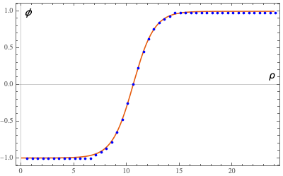
As we stated in the introduction, the purpose if this study is not to recover these classical instanton solutions for the tunnelling per se, as they are well-known, but rather to demonstrate that the corresponding field-theory configuration can be suitably encoded into a quantum annealer. Once we have established this as a working principle, one could even envisage testing for the above behaviour directly. Therefore we will in what follows focus on using a quantum annealer to recover the simple $c=0$ solution required for the thin-wall regime, as a proof of principle. We will therefore set ourselves the task of minimising the corresponding action integral,

$$S_{1}\,=\,\int_{0}^{\infty}d\rho\penalty\ \frac{1}{2}{\dot{\phi}^{2}}+U(\phi)\penalty\ ,$$

(7)

which should yield a solution of the form shown in Fig.2b.

Let us start with the central problem, which is how to formulate a continuous scalar field theory on quantum annealers. A quantum annealer is based on the adiabatic theorem of quantum mechanics, which implies that a physical system will remain in the ground state if a given perturbation acts slowly enough, and if there is a gap between the ground state and the rest of the system’s energy spectrum [24]. For the annealer to provide a solution to a mathematical problem, e.g. the calculation of $\phi(\rho)$ for Eq. 7, we have to find a mapping such that the expectation value of its Hamiltonian can be identified with its solution, i.e. that it allows in this example to identify

$$\phi(\rho)\iff\lim_{t\to 0}\left<\mathcal{H}_{\mathrm{QA}}(t)\right>.$$

(8)

The form of the Hamiltonian available to a quantum annealer is that of a general Ising model, in addition to a time-dependent transverse field:

$$\mathcal{H}_{\mathrm{QA}}(t)=\sum_{i}\sum_{j}J_{ij}\sigma_{i}^{Z}\sigma_{j}^{Z}+\sum_{i}h_{i}\sigma_{i}^{Z}+\Delta(t)\sum_{i}\sigma_{i}^{X}\penalty\ ,$$

(9)

where $\sigma^{Z}_{i}=\left(\begin{array}[]{cc}1&0\\ 0&-1\end{array}\right)$ ($\sigma^{Z}|0\rangle=|0\rangle$, $\sigma^{Z}|1\rangle=-|1\rangle$) is the Pauli $Z$ operator, with the subscript indicating which spin it acts upon, and $\sigma^{X}$ is its friend pointing in the $X$-direction. The gradual decrease of $\Delta(t)\to 0$ from a large value should drive the system into the ground state of the time-independent part of the Hamiltonian, and this is where we will put the field theory:

$$\mathcal{H}=\sum_{i}\sum_{j}J_{ij}\sigma^{Z}_{i}\sigma^{Z}_{j}+\sum_{i}h_{i}\sigma^{Z}_{i}\penalty\ .$$

(10)

It is worth noting that the couplings $J_{ij}$ and $h_{i}$ could also be adiabatically adjusted in the annealing process, and this could ultimately be used to adjust the potential $U(\phi)$ of a system in the quantum annealer so as to observe tunnelling, assuming it can be encoded. We will further split the Hamiltonian into three generic pieces, as

$$\mathcal{H}\penalty\ =\penalty\ \mathcal{H}^{(\mathrm{chain})}+\mathcal{H}^{\mathrm{(QFT)}}+\mathcal{H}^{\mathrm{(BC)}}.$$

(11)

Here, $\mathcal{H}^{\mathrm{(QFT)}}$ is the Hamiltonian corresponding to the minimisation of the action in Eq. 7 and $\mathcal{H}^{\mathrm{(BC)}}$ is a Hamiltonian that we add to enforce the boundary conditions²² 2 For a classical neural network-based approach to solving Eq. 2 by treating it as an optimisation problem see [46]..

However our first task is to encode continuous field values over a continuous domain, with only the discrete Ising model to hand: this is what ${\mathcal{H}}^{(\mathrm{chain})}$ is for. We begin by splitting the radius variable $\rho$ into $M\gg 1$ discrete values and the field value at the $\ell$’th position into $N\gg 1$ discrete values:

$$\begin{array}[]{lll}\rho_{\ell}&\,=\,\ell\nu&=\penalty\ \penalty\ \nu\ldots M\nu\\ \phi(\rho_{l})&\,=\,\phi_{0}+\alpha_{l}\xi&=\penalty\ \penalty\ \phi_{0}+\xi\,\ldots\,\phi_{0}+N\xi\,,\end{array}$$

where in the present context one might for example take a fiducial value $\phi_{0}\approx-a$ and $\xi=2a/N$, with $M\nu=\Delta\rho$. Thus our Ising interaction $J_{ij}$ is an $(MN)\times(MN)$ matrix, while $h_{i}$ is an $(NM)$-vector.

We must now separate those spins in the annealer that correspond to fields at different values of $\ell$, effectively splitting $J_{ij}$ and $h_{i}$ into $N\times N$ sub-blocks. To do this we will utilise the Ising-chain domain wall representation introduced in [47]. That is for every position $\ell$ we add to the Hamiltonian

$$\mathcal{H_{\ell}^{\mathrm{(chain)}}}=-\Lambda\left(\sum_{j=1}^{N-1}\sigma_{\ell N+j}^{Z}\sigma_{\ell N+j+1}^{Z}-\sigma^{Z}_{\ell N+1}+\sigma^{Z}_{\ell N+N}\right)\penalty\ .$$

(12)

As shown in [47], taking $\Lambda$ to be much larger than every other energy scale in the overall Hamiltonian, these terms will constrain the system to remain in the ground subspace of the Hamiltonian, where exactly one spin position, $\alpha_{\ell}$ say, is frustrated for each $\ell$. These states are of the form

$$|11...100...0\rangle_{\ell}\penalty\ \implies\penalty\ \phi(\rho_{\ell})\,=\,\phi_{0}+\alpha_{\ell}\xi\penalty\ ,$$

(13)

where in the above the discretised field value is represented by the position $\alpha_{\ell}$ of the frustrated domain wall. Conversely the field value at the $\ell$’th position can be found by making the measurement

$\displaystyle\phi(\rho_{\ell})\,$

$\displaystyle=\,\frac{1}{2}\sum_{j=1}^{N-1}(\phi_{0}+j\xi)\,\langle\sigma^{Z}_{\ell N+j+1}-\sigma^{Z}_{\ell N+j}\rangle\penalty\ ,$

(14)

which only receives a contribution from frustrated spin position with $j=\alpha_{\ell}$. For later, it is useful to note that this is equivalent to

$\displaystyle\phi(\rho_{\ell})\,$

$\displaystyle=\,\phi_{0}+\frac{N\xi}{2}-\frac{\xi}{2}\sum_{j=1}^{N}\,\langle\sigma^{Z}_{\ell N+j}\rangle\penalty\ .$

(15)

In terms of $J_{ij}$ and $h_{i}$, adding the full set of Ising-chain Hamiltonians given by Eq.(12) corresponds to

$\displaystyle J_{\ell N+i,mN+j}^{(\text{chain})}$

$\displaystyle=-\frac{\Lambda}{2}\,\delta_{\ell m}\,\otimes\,\left(\begin{array}[]{cccccc}0&1\\ 1&0&1\\ &1&0\\ &&&\ddots\\ &&&&0&1\\ &&&&1&0\end{array}\right)_{ij}\penalty\ ,$

and an $h$ that is independent of $\ell$,

$\displaystyle h^{(\text{chain})}_{\ell N+j}$

$\displaystyle=\Lambda\,(\delta_{j1}-\delta_{jN})\penalty\ .$

(22)

This separates the system of spins into blocks of size $N$, each of which represents a field value.

Moving on to $\mathcal{H}^{(\mathrm{Q}FT)}$, the potential is somewhat easier to deal with than the kinetic terms, because it can be encoded entirely in $h_{i}$. This is only to be expected because the $\phi_{\ell}$ are independent of each other in the potential which gives entirely localised contributions to the Hamiltonian. The value of $U(\phi(\rho_{\ell}))$ at each point follows directly from Eq.(14):

$$U(\phi(\rho_{\ell}))\,=\,\frac{1}{2}\sum_{j=1}^{N-1}U(\phi_{0}+j\xi)\,\langle\sigma^{Z}_{\ell N+j+1}-\sigma^{Z}_{\ell N+j}\rangle\penalty\ .$$

(23)

This yields an additional contribution to the $h$ which is also independent of $\ell$: that is for all $\ell$ we have

$\displaystyle h_{N\ell+j}^{(\text{QFT})}\,$

$\displaystyle=\,\left\{\begin{array}[]{ll}\vskip 5.69046pt{\frac{\nu}{2}\left(U(\phi_{0}+(j-1)\xi)-U(\phi_{0}+j\xi)\right)}\penalty\ ;&{j<N}\\ {\frac{\nu}{2}U(\phi_{0}+(N-1)\xi)}\penalty\ ;&{j=N}\end{array}\right.$

It can also be convenient to write this in terms of $U$ derivatives as

$\displaystyle h_{N\ell+j}^{(\text{QFT})}\,$

$\displaystyle=\,\left\{\begin{array}[]{ll}\vskip 5.69046pt{-\frac{\nu\xi}{2}U^{\prime}(\phi_{0}+j\xi)}\penalty\ ;&{j<N}\\ {\frac{\nu}{2}\left(U(\phi_{0}+(N-1)\xi)\right)}\penalty\ ;&{j=N}\,,\end{array}\right.$

which correctly gives $\phi(\rho_{\ell})$ of Eq.(15) in the event that we take $U(\phi)=\phi$ (because we know that $\sigma_{\ell N}^{Z}=1$). Note that in a system with arbitrary $c\neq 0$, we would need to evaluate $h^{(U)}\equiv\int d\rho\rho^{c}U$, so that $h_{\ell N+i}$ would acquire a prefactor of $(\ell\nu)^{c}.$

Up to this point the $M$-factors have been inert and there has been no coupling between the fields at different positions in $\rho_{\ell}$. At this stage the system would simply relax to $M$ decoupled values of $\phi(\rho_{\ell})$ that minimise $U$ in either one of its two vacua. This changes once we include the derivatives in the kinetic terms, which contribute to the bilinear interactions, $J$. These terms are discretised in $\rho$ as

$$S_{KE}\equiv\int_{0}^{\Delta\rho}d\rho\frac{1}{2}\dot{\phi}^{2}=\lim_{M\rightarrow\infty}\sum_{\ell=1}^{M}\frac{1}{2\nu}\left(\phi(\rho_{\ell+1})-\phi(\rho_{\ell})\right)^{2},$$

(28)

where $\nu=\Delta\rho/M$ scales so as to keep $\Delta\rho$ constant. Inserting the discrete representation of the field values as well using Eq.(15), we find

	$\displaystyle S_{KE}$	$\displaystyle=\sum_{\ell=1}^{M-1}\sum_{ij}^{N-1}\frac{\xi^{2}}{8\nu}\left[\sigma_{(\ell+1)N+i}^{Z}-\sigma_{\ell N+i}^{Z}\right]\times\qquad\qquad$			(29)
		$\displaystyle\qquad\qquad\qquad\qquad\qquad\left[\sigma_{(\ell+1)N+j}^{Z}-\sigma_{\ell N+j}^{Z}\right].$

Hence the bilinear terms receive the additional contribution:

$$\mathord{\raise 0.49991pt\hbox{$\displaystyle J$}}_{\ell N+i,mN+j}^{(\text{QFT})}=\frac{\xi^{2}}{8\nu}\,\left(\begin{array}[]{cccccc}1&-1\\ -1&2&-1\\ &-1&2&-1\\ &&&\ddots\\ &&&-1&2&-1\\ &&&&-1&1\end{array}\right)_{\ell m}$$

(30)

Now it is the $N\times N$ indices that are inert, because every $i$ couples to every $j$.

Note that the diagonal parts of Eq.30 could be embedded in the $h_{i}$ terms, using the fact that for valid single domain wall states we have $\langle\sigma^{Z}_{\ell N+i}\sigma^{Z}_{\ell N+j}\rangle=\langle\sigma^{Z}_{\ell N+j}-\sigma^{Z}_{\ell N+i}+1\rangle$ for $j>i$. As bilinear terms may be hard to engineer on real devices, this may be desirable, but for the present study it is more convenient to keep the kinetic terms entirely.

Finally we must add terms to enforce a boundary condition. In the $c=0$ case it is sufficient to fix the endpoints of the solution in the two minima (so that, at the risk of confusion, the instanton solution itself approximates a physical domain wall). This can be done by adding a term ${\cal H}^{(BC)}=\frac{\Lambda^{\prime}}{2}(\phi(0)+a)^{2}+\frac{\Lambda^{\prime}}{2}(\phi(\rho_{M})-a)^{2}$ with $\Lambda^{\prime}$ being some other large parameter. This is simply an extra contribution to $h$ which follows directly from Eq.(III), of the form

$\displaystyle h_{N\ell+j}^{(\text{BC})}\,$

$\displaystyle=\,\left\{\begin{array}[]{ll}\vskip 5.69046pt-{\Lambda^{\prime}}(\phi_{0}+j\xi+a)\penalty\ ;&{\ell=1},\forall j\\ -{\Lambda^{\prime}}(\phi_{0}+j\xi-a)\penalty\ ;&{\ell=M-1,\forall j}\penalty\ .\end{array}\right.$

Together with Eqs.(III,22,III,30), this completes the encoding of the field theory problem of Eq.(7).

In Sec. III we have devised a method which encodes the problem of finding a solution to a quantum field theoretical problem, i.e. of finding a solution to Eq. 7, into finding the ground state of the Hamiltonian of an Ising model. The latter can then be given an interpretation as the solution to Eq. 7 through Eq. 13, for each $\rho_{l}$ with $l\in[1,...,M]$. To show that our approach is valid and converges to the correct solution $\phi(\rho)$, we now implement the method onto various annealing samplers, as provided by D-Wave [48].

The quantum states are characterised by $NM$-tuples of the form $\left|11...100...0\right>$ and the Hilbert space of the Ising model is therefore $2^{NM}$ dimensional. Sampling such a large vector space classically, with an exact sampler, while calculating the expectation value $\left<\mathcal{H}\right>$ for each state quickly becomes a computationally prohibitive task for $NM\gg 20$. Conversely, a discretisation with $NM\lesssim 20$ cannot give a reasonable approximation for the derivatives of Eq. 28.

Yet, not unlike protein-folding, in which a unique ground state is selected from an estimated number of $3^{300}$ so-called conformations within microseconds (known as Levinthal’s paradox [49]), a quantum annealer can in principle find a ground state of a Hamiltonian acting on a highly complex Hilbert space on a similar time scale, assuming there is a gap between the ground state and the other states of the system.

While the next generation of annealing processors will have approximately 5,000 qubits, they will have limited connectivity [50]. Therefore in order to accommodate the more general Ising model required for our encoding, we resorted to a hybrid asynchronous decomposition sampler (the Kerberos solver [51]), which can solve problems of arbitrary structure and size. To find the ground state efficiently, it applies in parallel classical tabu search algorithms, simulated annealing and D-Wave subproblem sampling on variables that have high-energy impact. Using this method we calculate the solution $\phi(\rho)$ to Eq. 7 for $N=M=50$ in Fig. 2b.

Consequently, near-term applications of quantum devices can significantly enhance our ability to perform highly complex quantum field theoretical calculations. Focussing on the problem of calculating the classical instanton solution in Sec. II, we have proposed a method to formulate such problems as an Ising model in Sec. III, which we have solved on a D-Wave quantum annealer. Our method is highly flexible and can straightforwardly be generalised to encode any multi-dimensional differo-integral equation as an Ising model.

References

- Feynman [1982] R. P. Feynman, “Simulating physics with computers”, Int. J. Theor. Phys. 21 (1982) 467–488, [,923(1981)].
- Zalka [1998] C. Zalka, “Efficient simulation of quantum systems by quantum computers”, Proc. Roy. Soc. Lond. A454 (1998) 313–322, arXiv:quant-ph/9603026.
- Jordan et al. [2012] S. P. Jordan, K. S. M. Lee, and J. Preskill, “Quantum Algorithms for Quantum Field Theories”, Science 336 (2012) 1130–1133, arXiv:1111.3633.
- Jordan et al. [2011] S. P. Jordan, K. S. M. Lee, and J. Preskill, “Quantum Computation of Scattering in Scalar Quantum Field Theories”, arXiv:1112.4833, [Quant. Inf. Comput.14,1014(2014)].
- García-Álvarez et al. [2015] L. García-Álvarez, J. Casanova, A. Mezzacapo, I. L. Egusquiza, L. Lamata, G. Romero, and E. Solano, “Fermion-Fermion Scattering in Quantum Field Theory with Superconducting Circuits”, Phys. Rev. Lett. 114 (2015), no. 7, 070502, arXiv:1404.2868.
- Jordan et al. [2014] S. P. Jordan, K. S. M. Lee, and J. Preskill, “Quantum Algorithms for Fermionic Quantum Field Theories”, arXiv:1404.7115.
- Beverland et al. [2016] M. E. Beverland, O. Buerschaper, R. Koenig, F. Pastawski, J. Preskill, and S. Sijher, “Protected gates for topological quantum field theories”, J. Math. Phys. 57 (2016), no. 2, 022201, arXiv:1409.3898.
- Jordan et al. [2017] S. P. Jordan, H. Krovi, K. S. M. Lee, and J. Preskill, “BQP-completeness of Scattering in Scalar Quantum Field Theory”, arXiv:1703.00454.
- Hamed Moosavian and Jordan [2018] A. Hamed Moosavian and S. Jordan, “Faster Quantum Algorithm to simulate Fermionic Quantum Field Theory”, Phys. Rev. A98 (2018), no. 1, 012332, arXiv:1711.04006.
- Preskill [2018] J. Preskill, “Simulating quantum field theory with a quantum computer”, PoS LATTICE2018 (2018) 024, arXiv:1811.10085.
- Lamm and Lawrence [2018] H. Lamm and S. Lawrence, “Simulation of Nonequilibrium Dynamics on a Quantum Computer”, Phys. Rev. Lett. 121 (2018), no. 17, 170501, arXiv:1806.06649.
- Yeter-Aydeniz et al. [2019] K. Yeter-Aydeniz, E. F. Dumitrescu, A. J. McCaskey, R. S. Bennink, R. C. Pooser, and G. Siopsis, “Scalar Quantum Field Theories as a Benchmark for Near-Term Quantum Computers”, Phys. Rev. A99 (2019), no. 3, 032306, arXiv:1811.12332.
- Bauer et al. [2019] C. W. Bauer, W. A. De Jong, B. Nachman, and D. Provasoli, “A quantum algorithm for high energy physics simulations”, arXiv:1904.03196.
- Moosavian et al. [2019] A. H. Moosavian, J. R. Garrison, and S. P. Jordan, “Site-by-site quantum state preparation algorithm for preparing vacua of fermionic lattice field theories”, arXiv:1911.03505.
- Gustafson et al. [2019] E. Gustafson, P. Dreher, Z. Hang, and Y. Meurice, “Real time evolution of a one-dimensional field theory on a 20 qubit machine”, arXiv:1910.09478.
- Klco and Savage [2019] N. Klco and M. J. Savage, “Systematically Localizable Operators for Quantum Simulations of Quantum Field Theories”, arXiv:1912.03577.
- Harmalkar et al. [2020] NuQS Collaboration, S. Harmalkar, H. Lamm, and S. Lawrence, “Quantum Simulation of Field Theories Without State Preparation”, arXiv:2001.11490.
- Wei et al. [2019] A. Y. Wei, P. Naik, A. W. Harrow, and J. Thaler, “Quantum Algorithms for Jet Clustering”, arXiv:1908.08949.
- Matchev et al. [2020] K. T. Matchev, P. Shyamsundar, and J. Smolinsky, “A quantum algorithm for model independent searches for new physics”, arXiv:2003.02181.
- Arrighi et al. [2018] P. Arrighi, G. D. Molfetta, I. Márquez-Mártin, and A. Pérez, “The dirac equation as a quantum walk over the honeycomb and triangular lattices”, Physical Review A 97 (2018) 062111, arXiv:1803.01015.
- Márquez-Mártin et al. [2018] I. Márquez-Mártin, P. Arnault, G. D. Molfetta, and A. Pérez, “Electromagnetic lattice gauge invariance in two-dimensional discrete-time quantum walks”, Physical Review A 98 (2018) 032333, arXiv:1808.04488.
- Jay et al. [2019] G. Jay, F. Debbasch, and J. B. Wang, “Dirac quantum walks on triangular and honeycomb lattices”, Physical Review A 99 (2019) 032113, arXiv:1803.01304.
- Molfetta and Arrighi [2020] G. D. Molfetta and P. Arrighi, “A quantum walk with both a continuous-time limit and a continuous-spacetime limit”, Quantum Inf Process 19 (2020) 47, arXiv:1906.04483.
- Farhi et al. [2000] E. Farhi, J. Goldstone, S. Gutmann, and M. Sipser, “Quantum computation by adiabatic evolution”. ariv:quant-ph/0001106, 2000.
- Neven et al. [2009] H. Neven, V. S. Denchev, M. Drew-Brook, J. Zhang, W. G. Macready, and G. Rose, “Nips 2009 demonstration: Binary classification using hardware implementation of quantum annealing”, 2009.
- Finilla et al. [1994] A. B. Finilla, M. A. Gomez, C. Sebenik, and J. D. Doll, “Quantum annealing: A new method for minimizing multidimensional functions”, Chem. Phys. Lett. 219 (1994) 343.
- Kadowaki and Nishimori [1998] T. Kadowaki and H. Nishimori, “Quantum annealing in the transverse ising model”, Phys. Rev. E 58 (1998) 5355.
- Brooke et al. [1999] J. Brooke, D. Bitko, T. F. Rosenbaum, and G. Aeppli, “Quantum annealing of a disordered magnet”, Science 284 (1999), no. 5415, 779–781.
- et. al [2013] N. G. D. et. al, “Thermally assisted quantum annealing of a 16-qubit problem”, Nature Communications 4 (2013) 1903.
- Lanting et al. [2014] T. Lanting, A. J. Przybysz, A. Y. Smirnov, F. M. Spedalieri, M. H. Amin, A. J. Berkley, R. Harris, F. Altomare, S. Boixo, P. Bunyk, N. Dickson, C. Enderud, J. P. Hilton, E. Hoskinson, M. W. Johnson, E. Ladizinsky, N. Ladizinsky, R. Neufeld, T. Oh, I. Perminov, C. Rich, M. C. Thom, E. Tolkacheva, S. Uchaikin, A. B. Wilson, and G. Rose, “Entanglement in a quantum annealing processor”, Phys. Rev. X 4 May (2014) 021041.
- Albash et al. [2015] T. Albash, W. Vinci, A. Mishra, P. A. Warburton, and D. A. Lidar, “Consistency tests of classical and quantum models for a quantum annealer”, Phys. Rev. A 91 (2015), no. 042314,.
- Albash and Lidar [2018] T. Albash and D. A. Lidar, “Adiabatic quantum computing”, Rev. Mod. Phys. 90 (2018), no. 015002,.
- Boixo et al. [2016] S. Boixo, V. N. Smelyanskiy, A. Shabani, S. V. Isakov, M. Dykman, V. S. Denchev, M. H. Amin, A. Y. Smirnov, M. Mohseni, and H. Neven, “Computational multiqubit tunnelling in programmable quantum annealers”, Nature Communications 7 (2016), no. 10327,.
- Chancellor et al. [2016] N. Chancellor, S. Szoke, W. Vinci, G. Aeppli, and P. A. Warburton, “Maximum–entropy inference with a programmable annealer”, Scientific Reports 6 (2016), no. 22318,.
- Benedetti et al. [2016] M. Benedetti, J. Realpe-Gómez, R. Biswas, and A. Perdomo-Ortiz, “Estimation of effective temperatures in quantum annealers for sampling applications: A case study with possible applications in deep learning”, Phys. Rev. A 94 Aug (2016) 022308.
- Muthukrishnan et al. [2016] S. Muthukrishnan, T. Albash, and D. A. Lidar, “Tunneling and speedup in quantum optimization for permutation-symmetric problems”, Phys. Rev. X 6 Jul (2016) 031010.
- Lanting [2017] T. Lanting, “The D-Wave 2000Q Processor”, 2017. presented at AQC 2017.
- Chancellor [2017] N. Chancellor, “Modernizing quantum annealing using local searches”, New Journal of Physics 19 feb (2017) 023024.
- Harris et al. [2018] R. Harris, Y. Sato, A. J. Berkley, M. Reis, F. Altomare, M. H. Amin, K. Boothby, P. Bunyk, C. Deng, C. Enderud, S. Huang, E. Hoskinson, M. W. Johnson, E. Ladizinsky, N. Ladizinsky, T. Lanting, R. Li, T. Medina, R. Molavi, R. Neufeld, T. Oh, I. Pavlov, I. Perminov, G. Poulin-Lamarre, C. Rich, A. Smirnov, L. Swenson, N. Tsai, M. Volkmann, J. Whittaker, and J. Yao, “Phase transitions in a programmable quantum spin glass simulator”, Science 361 (2018), no. 6398, 162–165.
- King et al. [2018] A. D. King, J. Carrasquilla, J. Raymond, I. Ozfidan, E. Andriyash, A. Berkley, M. Reis, T. Lanting, R. Harris, F. Altomare, K. Boothby, P. I. Bunyk, C. Enderud, A. Fréchette, E. Hoskinson, N. Ladizinsky, T. Oh, G. Poulin-Lamarre, C. Rich, Y. Sato, A. Y. Smirnov, L. J. Swenson, M. H. Volkmann, J. Whittaker, J. Yao, E. Ladizinsky, M. W. Johnson, J. Hilton, and M. H. Amin, “Observation of topological phenomena in a programmable lattice of 1,800 qubits”, Nature 560 (2018), no. 7719, 456–460.
- King et al. [2019] A. D. King, J. Raymond, T. Lanting, S. V. Isakov, M. Mohseni, G. Poulin-Lamarre, S. Ejtemaee, W. Bernoudy, I. Ozfidan, A. Y. Smirnov, M. Reis, F. Altomare, M. Babcock, C. Baron, A. J. Berkley, K. Boothby, P. I. Bunyk, H. Christiani, C. Enderud, B. Evert, R. Harris, E. Hoskinson, S. Huang, K. Jooya, A. Khodabandelou, N. Ladizinsky, R. Li, P. A. Lott, A. J. R. MacDonald, D. Marsden, G. Marsden, T. Medina, R. Molavi, R. Neufeld, M. Norouzpour, T. Oh, I. Pavlov, I. Perminov, T. Prescott, C. Rich, Y. Sato, B. Sheldan, G. Sterling, L. J. Swenson, N. Tsai, M. H. Volkmann, J. D. Whittaker, W. Wilkinson, J. Yao, H. Neven, J. P. Hilton, E. Ladizinsky, M. W. Johnson, and M. H. Amin, “Scaling advantage in quantum simulation of geometrically frustrated magnets”, 2019.
- Coleman [1977] S. R. Coleman, “The Fate of the False Vacuum. 1. Semiclassical Theory”, Phys. Rev. D15 (1977) 2929–2936, [Erratum: Phys. Rev.D16,1248(1977)].
- Callan and Coleman [1977] C. G. Callan, Jr. and S. R. Coleman, “The Fate of the False Vacuum. 2. First Quantum Corrections”, Phys. Rev. D16 (1977) 1762–1768.
- Coleman [1988] S. Coleman, “Aspects of symmetry: Selected erice lectures”, Cambridge University Press, 1988.
- Linde [1983] A. D. Linde, “Decay of the False Vacuum at Finite Temperature”, Nucl. Phys. B216 (1983) 421, [Erratum: Nucl. Phys.B223,544(1983)].
- Piscopo et al. [2019] M. L. Piscopo, M. Spannowsky, and P. Waite, “Solving differential equations with neural networks: Applications to the calculation of cosmological phase transitions”, Phys. Rev. D100 (2019), no. 1, 016002, arXiv:1902.05563.
- Chancellor [2019] N. Chancellor, “Domain wall encoding of discrete variables for quantum annealing and QAOA”, Quantum Science and Technology 4 aug (2019) 045004.
- D-Wave [2019] D-Wave, “D-wave systems inc. website”. http://www.dwavesys.com/, 2019. Accessed: 2019-05-03.
- Levinthal [1969] C. Levinthal, “How to fold graciously”, Mossbauer Spectroscopy in Biological Systems: Proceedings of a meeting held at Allerton House, Monticello, Illinois, 01 1969.
- Boothby et al. [2020] K. Boothby, P. Bunyk, J. Raymond, and A. Roy, “Next-generation topology of d-wave quantum processors”, 02 2020.
- D-Wave Systems Inc. [accessed: 15 Mar 2020 https://docs.ocean.dwavesys .com/en/latest/docs_hybrid/sdk_index.html] D-Wave Systems Inc., “dwave-hybrid documentation”, accessed: 15 Mar 2020 https://docs.ocean.dwavesys .com/en/latest/docs_hybrid/sdk_index.html.