A Nanoscale Coherent Light Source
Abstract
Generically, a laser is composed of an optical resonator coupled to a gain medium. If the light amplification via stimulated emission dominates the mirror losses, the emitted light is coherent. Recent studies have shown that sub-wavelength sized rings of quantum emitters possess subradiant eigenmodes which mimic high- optical resonators. We add a continuously pumped atom as a gain medium in the ring’s center creating a minimalistic coherent light source. The system behaves like a thresholdless laser, featuring a narrow linewidth well below the natural linewidth of the constituent atoms.
pacs
42.50.Ar, 42.50.Lc, 42.72.-gI Introduction
Conventional lasers consist of an optical cavity filled with a gain medium, typically comprised by an ensemble of energetically inverted emitters amplifying the light field via stimulated emission. Pioneering experiments have realized lasers with the most minimalistic gain medium yet, a single atom Brune et al. 1987; McKeever et al. 2003; Davidovich et al. 1987; Walther 1988; An et al. 1994; Astafiev et al. 2007; Rastelli and Governale 2019; Löffler et al. 1997. Corresponding theoretical quantum models have already been studied extensively for several decades Meschede et al. 1985; Mu and Savage 1992; Pellizzari and Ritsch 1994; Salzburger et al. 2005. Standard models of a single-atom laser still feature a macroscopic optical resonator supporting the corresponding laser light mode. Technically, the noise of the cavity mirrors is a substantially limiting factor for the frequency stability of a laser. This can be reduced when working in the bad cavity regime, such that the coherence is stored in the atomic dipoles rather than the light field. In such superradiant lasers Meiser et al. 2009; Meiser and Holland 2010; Bedoui et al. 2012; Maier et al. 2014; Hotter et al. 2019 the properties of the emitted light are governed by the gain medium rather than the resonator.
In this work we go one step further removing the cavity altogether and consider a nano-scale system where atomic quantum emitters provide for the necessary gain while simultaneously acting as a resonator. Thus, in principle, the size of the entire setup can be reduced to even below the order of the laser wavelength. Such a device is characterized solely by the spectral properties of the atoms.

As discovered recently, tailored dipole-coupled atomic arrays possess collective eigenmodes with a very long lifetime demonstrating analogous characteristics to a high- optical cavity mode Moreno-Cardoner et al. 2019; Manzoni et al. 2018. Such arrangements could be implemented, e.g. by means of optical tweezers Barredo et al. 2016; Barredo et al. 2018; Wang et al. 2019 or superconducting qubit setups operating in the microwave regime Blais et al. 2004. We study the prospects of implementing a minimalistic sub-wavelength sized laser by incoherently pumping some of the dipoles in such a nano array. As our generic setup we consider a single atom placed in the center of a small ring comprised of identical emitters. The collective coupling to the other emitters in the ring is mediated by virtual photon exchange through the electromagnetic vacuum Lehmberg 1970; Hood et al. 2016; Astafiev et al. 2007. The collective eigenmodes of the outer ring take on the role of a resonator mode.
We show that such a minimal model constitutes a steady-state coherent light source with a spectral linewidth well below the single atom decay rate. Therefore, it can be viewed as a minimal implementation of a laser. Depending on the number of atoms and the configuration of the array, the collective nature of the dipole-dipole couplings leads to strong quantum correlations within the atoms and an inherent emission of a coherent field. Optimal operation is achieved when the collective state in the ring atoms features a single subradiant excitation only.
II Model
We consider identical two-level atoms with excited state and ground state each, separated in frequency by and arranged in a ring geometry at an inter-atomic distance of . An additional gain atom is placed in the center of the ring as depicted in Fig. 1a and is assumed to be pumped to its upper level incoherently at a rate (after having eliminated auxiliary levels). The corresponding raising (lowering) operators of the th atom are for (the index corresponds to the central, pumped atom). The excited state is subject to spontaneous emission with a rate . All transition dipoles are chosen such that they point in -direction.
At the considered distances, the fields emitted by each of the atoms interfere resulting in effective dipole-dipole interactions Lehmberg 1970, so that the atomic ring acts like a resonator Moreno-Cardoner et al. 2019 coupled to the gain atom in its center.
Using standard quantum optical techniques Gardiner and Zoller 2004 we obtain a master equation for the internal dynamics of the emitters, where the Lindblad term describing the incoherent pumping of the central atom is given by The corresponding Hamiltonian in a frame rotating at the atomic transition frequency is
| (1) |
while the Lindblad operator accounting for collective spontaneous emission reads
| (2) |
The collective coupling rates and are given as the real and imaginary part of the overlap of the transition dipole of the th atom with the electric field emitted by the th atom (see Eq. (10)).
The emitted electric field can be used to compute the field intensity as (see Eq. (11)), i.e.
| (3) |
III Continuous Collective Emission
Our goal is to find operating regimes where the system emits coherent light with a narrow linewidth. As the configuration is symmetric with respect to the coupling of the ring atoms to the gain atom in the center, we can expect the ring atoms to be driven into a symmetric excitation state given as
| (4) |
In accordance with standard laser theory we will target parameters for which a symmetric excitation of the ring atoms constitutes a good cavity, i.e. the radiative loss is sufficiently small. To this end, we study the stationary populations of different eigenstates of our Hamiltonian from Eq. (1) during a time evolution starting from the ground state as depicted in Fig. 2a.
Indeed, as shown in Fig. 2, we find that the two eigenstates involving the symmetric single-excitation state in the ring are occupied predominately at all times (except for the ground state). These states are given by
| (5) |
for , where and depend on the particular geometry with .
Note that the gain atom can only emit one photon into the ring at a time. Hence, the single-excitation manifold dominates the dynamics even for pump rates substantially larger than the single-atom decay rate. This is shown in Fig. 2b, where we plot the occupation probability of different eigenstates at steady state as a function of .
The fact that the ring does indeed form a resonator can be seen more clearly as follows. Let us assume that only the symmetric state in the ring is populated. Thus, we can rewrite the Hamiltonian in the subspace spanned by the ground and excited state of the gain atom in the center, as well as the ground state of the ring and its symmetric state obtaining (see Appendix)
| (6) |
where is the dipole energy shift of the symmetric state. Written like this, the Hamiltonian resembles the Jaynes-Cummings Hamiltonian with the ring taking on the role of the cavity mode. In this sense, the symmetric subspace lowering operator can be interpreted as the photon annihilation operator of our ”cavity”. The coupling between the gain atom and the cavity is then determined by .
If we neglect the dissipative coupling between the central atom and the atoms forming the ring, i.e. , we can rewrite the decay of the system as with
| (7a) | ||||
| (7b) | ||||
Minimizing the decay rate of the ring atoms is important, but in order to build up population within the ring we need an efficient coupling to the gain atom as well. In analogy to the Jaynes-Cummings model we thus define a cooperativity parameter (see Appendix) An efficient coherent coupling of the ring atoms to the gain atom is achieved when . As we can see in Fig. 4b, we reach this limit at extremely small distances or at a distance where is minimal (see Fig. 3). The cooperativity becomes large at since for the coherent coupling diverges. Yet, this is also the limit where the energy difference is large, which detunes the ring atoms from the gain atom. Furthermore, as we will show later, due to the superradiant loss of the ring in this limit the emitted light features thermal statistics rather than coherence. Consequently, we find that the optimal parameter regime indeed lies where the ring atoms show a subradiant behaviour, i.e. at the points highlighted in Fig. 3.

IV Photon Statistics and Spectral Properties
We have now identified a regime where our system resembles the typical setup of a single-atom laser. In order to study the statistical properties of the emitted light we calculate the normalized second-order correlation at zero time delay of the electric field intensity. In the far-field , where the intensity correlation function becomes independent of the position (see Appendix) and is given by
| (8) |
Coherent light exhibits a Poissonian statistic implying Gardiner and Zoller 2004; Mandel and Wolf 1995. Therefore, an operation in the previously identified parameter regimes leads to the emission of coherent light. In addition , we calculate the amount of emitted light, i.e.
In Fig. 5a we can see that points of coherent light emission where are achieved along a curve strongly resembling the optimal subradiance parameters shown in Fig. 3. The points where correspond to the situation where the gain atom decouples from the cavity atoms, since then only the single atom in the center can emit light. And, because it is not possible for a single atom to emit more than one photon at a time, we observe anti-bunching. However, this regime does not coincide with ”lasing” since the ring atoms are not occupied. Simultaneously, the intensity shown in Fig. 5b is small, but still finite when the emitted light is coherent. This is because coherences can only build up when the loss from the atoms in the ring is sufficiently low ( is small), which also reduces the amount of light emitted.
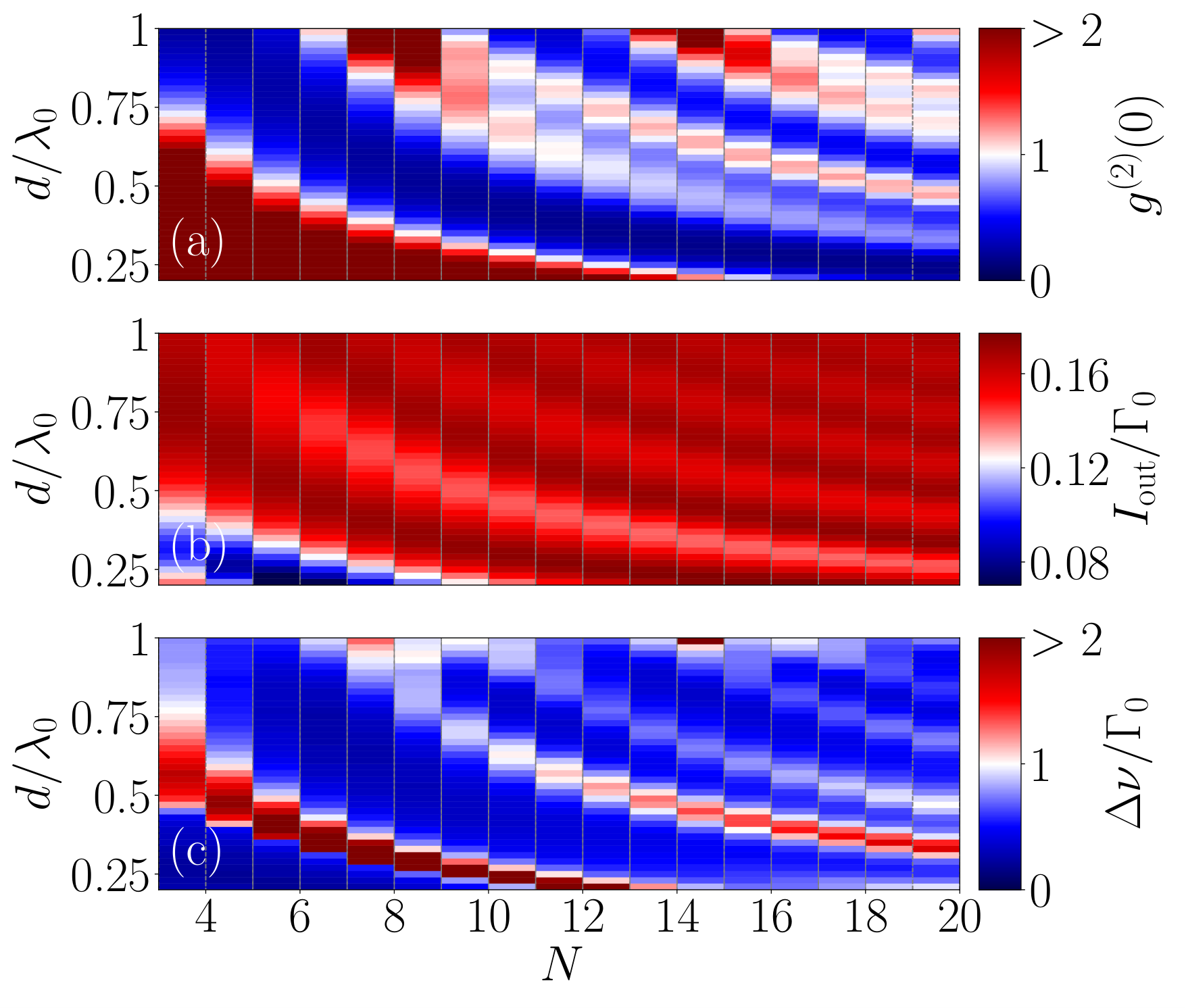
In order to analyze the emitted light in more detail, we compute its spectral linewidth. Therefore, we calculate the emission spectrum by means of the Wiener-Khinchin theorem (see eq. (21)) Carmichael 2009. It is given as the Fourier transform of the first-order coherence function, The spectrum has a Lorentzian shape, thus we compute the linewidth as the full width at half maximum (FWHM). In Fig. 5c, we show the linewidth as a function of and the interatomic distance . Once again, we find that the linewidth is small () at the points where the symmetric state is subradiant. It can be seen that in order to maintain coherent light emission the interatomic distances need to become smaller for an increasing number of atoms in a ring of constant radius.
Note, that in order to treat larger atom numbers in the above calculations we have truncated the Hilbert space at the second-excitation manifold (see Appendix). Since the single-excitation subspace usually dominates [as shown in Fig. 2], neglecting any state containing more than two excitations is well justified.
V Threshold-Less Behavior
In standard lasing models, coherent output light is achieved from a certain input power threshold on. Above threshold, the intensity of the emitted light increases drastically. In an effort to identify such a threshold in our setup, we compute the properties of the output light as a function of the pump strength of the gain atom.
The system does not exhibit a threshold. Such a threshold-less behavior has been observed in single-atom lasing setups McKeever et al. 2003. As we can see in Figs. 6a and 6b, the output intensity grows as soon as the pump rate becomes nonzero, rather than requiring a sufficiently large pump rate. At the same time, the photon statistics of the emitted field are Poissonian, i.e. , for arbitrarily low pumping rates (see Fig. 6c). The only point at which the photon statistics change is when the pump rate becomes large, , such that the emitted light starts to reproduce the thermal statistics of the input field. It can also be seen in Fig. 6a that above this point the output intensity is actually reduced. As one would expect, the linewidth of the emitted field is small () as long as the light is coherent (see Fig. 6d). When the incoherent pumping rate is increased, states outside the symmetric subspace are occupied, which leads to a slight increase in the linewidth. However, by increasing further, the linewidth decreases again and approaches as the central atom decouples from the ring atoms the light is emitted from the ring in the subradiant symmetric state.
VI Conclusions
We predict that a continuously pumped single atom surrounded by a nano-ring of identical atoms could act as a minimal, sub-wavelength sized implementation of a laser. Under suitable operating conditions the system will emit spatially and temporarily coherent light with Poisson statistics. Our analysis reveals a close analogy to the Jaynes-Cummings model, where the outer ring atoms take on the role of a high- cavity mode with the central atom providing for gain. The system works best when driven into a collective subradiant state with a single excitation. In this limit, spontaneous emission is suppressed and the operation strongly resembles the behavior of a threshold-less laser Boca et al. 2004. While the implementation of such a system in a pure form could be envisioned in optical tweezer arrays of neutral atoms Barredo et al. 2016, analogous setups based on quantum dots have been implemented and are already operational in the pulsed excitation regime le Feber et al. 2018.
Let us note here that there are no principal lower physical limits on the size of the system apart from the technical implementation of the structure and its pumping. Hence, very high density arrays of such lasers on a surface are possible.
Acknowledgements.
We acknowledge funding from the European Union’s Horizon 2020 research and innovation program under Grant Agreement No. 820404 iqClock (R. H., D. P. and H. R.) as well as from the Austrian Science Fund under project P29318-N27 (L. O.). The numerical simulations were performed with the open-source framework QuantumOptics.jl Krämer et al. 2018 and the graphs were produced with the open-source library Matplotlib Hunter 2007.References
- Brune et al. (1987) M. Brune, J. Raimond, P. Goy, L. Davidovich, and S. Haroche, Physical review letters 59, 1899 (1987).
- McKeever et al. (2003) J. McKeever, A. Boca, A. D. Boozer, J. R. Buck, and H. J. Kimble, Nature 425, 268 (2003).
- Davidovich et al. (1987) L. Davidovich, J. Raimond, M. Brune, and S. Haroche, Physical Review A 36, 3771 (1987).
- Walther (1988) H. Walther, Physica Scripta 1988, 165 (1988).
- An et al. (1994) K. An, J. J. Childs, R. R. Dasari, and M. S. Feld, Physical review letters 73, 3375 (1994).
- Astafiev et al. (2007) O. Astafiev, K. Inomata, A. Niskanen, T. Yamamoto, Y. A. Pashkin, Y. Nakamura, and J. S. Tsai, Nature 449, 588 (2007).
- Rastelli and Governale (2019) G. Rastelli and M. Governale, Phys. Rev. B 100, 085435 (2019).
- Löffler et al. (1997) M. Löffler, G. M. Meyer, and H. Walther, Phys. Rev. A 55, 3923 (1997).
- Meschede et al. (1985) D. Meschede, H. Walther, and G. Müller, Physical review letters 54, 551 (1985).
- Mu and Savage (1992) Y. Mu and C. M. Savage, Phys. Rev. A 46, 5944 (1992).
- Pellizzari and Ritsch (1994) T. Pellizzari and H. Ritsch, Journal of Modern Optics 41, 609 (1994).
- Salzburger et al. (2005) T. Salzburger, P. Domokos, and H. Ritsch, Physical Review A 72, 033805 (2005).
- Meiser et al. (2009) D. Meiser, J. Ye, D. Carlson, and M. Holland, Physical review letters 102, 163601 (2009).
- Meiser and Holland (2010) D. Meiser and M. Holland, Phys. Rev. A 81, 033847 (2010).
- Bedoui et al. (2012) S. Bedoui, M. Lopes, W. Nicolazzi, S. Bonnet, S. Zheng, G. Molnár, and A. Bousseksou, Phys. Rev. Lett. 109, 135702 (2012).
- Maier et al. (2014) T. Maier, S. Krämer, L. Ostermann, and H. Ritsch, Opt. Express 22, 13269 (2014).
- Hotter et al. (2019) C. Hotter, D. Plankensteiner, L. Ostermann, and H. Ritsch, Optics express 27, 31193 (2019).
- Moreno-Cardoner et al. (2019) M. Moreno-Cardoner, D. Plankensteiner, L. Ostermann, D. E. Chang, and H. Ritsch, Phys. Rev. A 100, 023806 (2019).
- Manzoni et al. (2018) M. Manzoni, M. Moreno-Cardoner, A. Asenjo-Garcia, J. V. Porto, A. V. Gorshkov, and D. Chang, New journal of physics 20, 083048 (2018).
- Barredo et al. (2016) D. Barredo, S. de Léséleuc, V. Lienhard, T. Lahaye, and A. Browaeys, Science 354, 1021 (2016).
- Barredo et al. (2018) D. Barredo, V. Lienhard, S. de Léséleuc, T. Lahaye, and A. Browaeys, Nature 561, 79 (2018).
- Wang et al. (2019) Y. Wang, S. Shevate, T. M. Wintermantel, M. Morgado, G. Lochead, and S. Whitlock, Preparation of hundreds of microscopic atomic ensembles in optical tweezer arrays (2019), arXiv:1912.04200 [physics.atom-ph] .
- Blais et al. (2004) A. Blais, R.-S. Huang, A. Wallraff, S. M. Girvin, and R. J. Schoelkopf, Physical Review A 69, 062320 (2004).
- Lehmberg (1970) R. Lehmberg, Phys. Rev. A 2, 883 (1970).
- Hood et al. (2016) J. D. Hood, A. Goban, A. Asenjo-Garcia, M. Lu, S.-P. Yu, D. E. Chang, and H. Kimble, Proceedings of the National Academy of Sciences 113, 10507 (2016).
- Gardiner and Zoller (2004) C. Gardiner and P. Zoller, Quantum noise: a handbook of Markovian and non-Markovian quantum stochastic methods with applications to quantum optics (SSBM, 2004).
- Mandel and Wolf (1995) L. Mandel and E. Wolf, Optical Coherence and Quantum Optics (Cambridge University Press, 1995).
- Carmichael (2009) H. Carmichael, An open systems approach to quantum optics: lectures presented at the Université Libre de Bruxelles, October 28 to November 4, 1991, Vol. 18 (Springer Science & Business Media, 2009).
- Boca et al. (2004) A. Boca, R. Miller, K. M. Birnbaum, A. D. Boozer, J. McKeever, and H. J. Kimble, Phys. Rev. Lett. 93, 233603 (2004).
- le Feber et al. (2018) B. le Feber, F. Prins, E. De Leo, F. T. Rabouw, and D. J. Norris, Nano letters 18, 1028 (2018).
- Krämer et al. (2018) S. Krämer, D. Plankensteiner, L. Ostermann, and H. Ritsch, Comput. Phys. Commun. 227, 109 (2018).
- Hunter (2007) J. D. Hunter, Comput. Sci. Eng. 9, 90 (2007).
- Jackson (2007) J. D. Jackson, Classical electrodynamics (John Wiley & Sons, 2007).
- Asenjo-Garcia et al. (2017a) A. Asenjo-Garcia, M. Moreno-Cardoner, A. Albrecht, H. J. Kimble, and D. E. Chang, Phys. Rev. X 7, 031024 (2017a).
- Asenjo-Garcia et al. (2017b) A. Asenjo-Garcia, J. D. Hood, D. E. Chang, and H. J. Kimble, Phys. Rev. A 95, 033818 (2017b).
VII Appendix
VII.1 Green’s Tensor
The collective coupling rates and are given as the real and imaginary part of the overlap of the transition dipole of the th atom with the electric field emitted by the th atom, i.e.
| (9a) | ||||
| (9b) | ||||
In the above, is the electromagnetic Green’s tensor of an oscillating dipole source in the vacuum Jackson 2007 which reads
| (10) | ||||
where and is the position unit vector, and is the spontaneous emission rate of a single atom.
The electric field operator can be obtained directly from the atomic operators Asenjo-Garcia et al. 2017a; Asenjo-Garcia et al. 2017b as
| (11) |
for the positive frequency component. This is the electric field generated by an ensemble of atoms at the position in the vacuum.
In order to arrive at the expression for the normalized second-order correlation function in the far-field we use the fact, that the overlap of the Green’s tensor with the atomic dipole becomes approximately independent for . In our case of identical two-level emitters polarized in -direction distributed in the -plane qq. (10) simplifies to
| (12) |
where and therefore upon normalization the second-order correlation function becomes independent of and .
VII.2 Symmetric Subspace
As mentioned in the main text, during the whole time evolution and for any incoherent pumping rate the ring is mainly in the symmetric state. This allows us to restrict ourselves to a subspace within the single-excitation manifold where either the central atom is excited or the symmetric state of the ring is populated. The Hilbert space is spanned by these two states and the ground state of the system, i.e.
| (13) |
Within this subspace the nonzero matrix elements of the Hamiltonian are given by
| (14a) | ||||
| (14b) | ||||
In turn, this allows us to rewrite the Hamiltonian in this basis as
| (15) |
where the subspace lowering operator is given by
| (16) |
If there is only a single excitation present in the system the Lindblad operator accounting for the collective spontaneous emission can be rewritten as
| (17) |
where the atomic density matrix in the steady state will live in the symmetric subspace, such that
| (18) |
Applying the Lindblad superoperator will yield the decay rates , and for , and , respectively. The collective decay between the central atom and the ring atoms will be approximately zero for the distances where and can be neglected as is discussed in the main text. The ring features the collective decay and the central atom independent spontaneous emission with the decay operators and respectively. Therefore the Lindblad term can be split into
| (19) |
This leads to a form of the Hamiltonian and Master equation which resembles the Jaynes-Cummings model, where the good cavity is given by the subradiant symmetric state of the ring atoms.
The definition of the cooperativity parameter can be understood as follows. As can be seen in , the coupling coefficient between the central atom and one of the ring atoms is given by , whereas the spontaneous decay into the vaccum modes for the center atom is simply . As analyzed in the main text, the ring atoms are predominately in the symmetric state with a collective decay rate for the parameters where the symmetric state is maximally subradiant. Interpreting the ring in the symmetric state as a cavity and the center atom as the gain medium leads to the definition of the cooperativity parameter .
VII.3 Truncating the Hilbert Space at Low Excitation
Concerning the scaling behaviour of the system a mean field treatment even with the inclusion of correlations to second order is not sufficient since the properties of the steady state strongly depend on correlations of higher orders in particular involves products of four operators. In order to analyze the scaling behaviour for a larger number of emitters in the ring we restrict the system to two excitations. This cut-off can only be a good approximation to the full model for small enough incoherent pumping rates . In fig. 7b the output intensity in the steady state of the reduced Hilbert space is compared to the full model for eight atoms in the ring and a good agreement can be found for . For , the intensity correlation function and the linewidth in fig. 7acd the pumping rate is and the interatomic distances are chosen along the white circles in fig. 3. The linewidth is well below with emitters in the ring and for distances where but reaches a minimum which is above .
VII.4 Computing the Spectrum
The spectrum we use in order to compute the linewidth via its FWHM is given by the Fourier Transform of the first-order correlation function. Similarly to the second-order correlation function, in the far-field this expression becomes independent of the geometry and is given by
| (20) |
The spectrum can then be computed via Carmichael 2009 as
| (21) |