A LAGRANGIAN PICTIONARYThanks: The second author was supported by an individual NSERC Discovery grant a Simons Fellowship and an Institute for Advanced Study fellowship grant.
1. Introduction.
The purpose of this paper is to describe a dictionary
in Lagrangian topology. As a by-product we obtain a tautological (in a sense to be explained) proof of a folklore conjecture (sometimes attributed to Kontsevich) claiming that the objects and structure of the derived Fukaya category can be represented through immersed Lagrangians. We also shed some new light on the dichotomy rigidity/flexibility that is at the heart of symplectic topology.
We focus on a symplectic manifold with compact or convex at infinity and we consider classes of (possibly immersed) Lagrangian submanifolds carrying also a variety of additional structures. In this paper the Lagrangians are exact and the choices of primitives are part of the structure.
1.1. Outline of the dictionary
1.1.1. Geometry
The geometric side of our dictionary, which does not appeal at any point to -holomorphic curves, consists of a class of Lagrangians, possibly immersed and marked (and endowed with additional structures). For an immersed Lagrangian , in generic position, a marking consists of a choice of a set of self intersection points with . The Lagrangians in are organized as a cobordism category , whose morphisms are represented by Lagrangian cobordisms belonging to a class . These are Lagrangians in whose projection onto is as in Figure 2. To such a category we associate a number of geometric operations. We then list a set of axioms governing them. If the category obeys these axioms we say that it has surgery models. The reason for this terminology is that the cobordisms associated to the classical operation of Lagrangian surgery [LS], [Pol], [BC1] are in some sense the simplest morphisms in our category, see also Figure 8. There is a natural equivalence relation , called cabling equivalence, on the morphisms of . The fact that the category has surgery models means that each morphism is equivalent to one coming from surgery (together with some other properties that we skip now). To understand this condition through an analogy, consider the path category of a Riemannian manifold, with objects the points of the manifold and with morphisms the Moore paths. In this case the equivalence relation is homotopy and the place of surgery morphisms is taken by geodesics. If has surgery models, then the quotient category
is triangulated. The triangulated structure appears naturally in this context because a surgery cobordism, resulting from the surgery operation, has three ends.
Cobordims are endowed with a natural measurement provided by their shadow - roughly the area of the connected “filling” of their projection onto [CS]. If has surgery models, then the triangulated structure of together with the weight provided by the shadow of cobordisms leads to the definition of a class of pseudo-metrics on called (shadow) fragmentation pseudo-metrics and denoted by [BCS]. Here is a family of objects in (it can be imagined as a family of generators with respect to the triangulated structure). Intuitively, the pseudo-distance between two objects and infimizes the weight of iterated cone-decompositions that express in terms of and of objects from the family . The category is called (strongly) rigid (or non-degenerate) in case, under some natural constraints on and a second such family (that can be viewed as a generic perturbation of ), the pseudo-metrics are non-degenerate.
1.1.2. Algebra
The algebraic side of the dictionary is mainly given by the derived Fukaya category associated to the embedded Lagrangians . The definition of this triangulated category [Sei] is an algebraically sophisticated application of -holomorphic curves techniques. The construction is only possible for Lagrangian submanifolds that are unobstructed [FOOO2]. Starting with the definition of Floer theory [Flo], a variety of constraints, often of topological type - such as exacteness, monotonicity etc - have been identified that are sufficient to ensure unobstructedness. Further unobstructedness conditions are now understood for Lagrangian immersions following the work of Akaho [Aka] and Akaho-Joyce [AJ].
1.2. Main result
In this framework, the central point of our dictionary is:
Theorem A.
There are certain classes , of exact, marked, unobstructed, immersed Lagrangian submanifolds and, respectively, cobordisms such that the category has surgery models and is rigid. Moreover, the quotient category is triangulated and its subcategory generated by the embedded Lagrangians is triangulated isomorphic to .
One way to look at this result is that if the class is small enough, the metric structure is non-degenerate but defining a triangulated structure on requires more objects than those in . On the other hand, if the class is too big, the triangulated structure is well defined but the expected metric is degenerate. However, the unobstructed class in the statement satisfies both properties - it is flexible enough so that triangulation is well-defined and, at the same time, it exhibits enough rigidity so that the metric is non-degenerate. Additionally, in this case the sub-category generated by embedded objects agrees with the derived Fukaya category and, thus, most algebraic structures typical in Lagrangian Floer theory can be reduced to understading how unobstructedness behaves with respect to the geometric operations appearing in our axioms.
Among immediate consequences of this result we see that the natural cobordism group generated by the embedded Lagrangians, modulo the relations given by the (possibly immersed) cobordisms in , is isomorphic to the Grothendieck group . In a different direction, because the Lagrangians in are unobstructed, there is a Donaldson category associated to this family and this category is isomorphic to .
The proof of Theorem A relates geometric constructions in to corresponding operations in . All objects and morphisms in are represented geometrically and all exact triangles in are represented by surgery. There are also relations between the pseudo-metrics and corresponding pseudo-metrics defined on the algebraic side by making use of action-filterered machinery.
This language also allows to formulate what today seems a very strong conjecture (or, maybe, just an intriguing question) that is a formal version in this context of Yasha Eliashberg’s claim that “there is no rigidity beyond -holomorphic curves”:
Conjecture/Question 1.
If has surgery models and is rigid, then it consists of unobstructed Lagrangians and, in particular, the morphisms in are Floer homology groups.
1.3. Some details
We discuss briefly here some of the main points in our approach.
1.3.1. Triangulation
As mentioned before, there is a simple reason why triangulated categories are the correct framework for organizing Lagrangian submanifolds. The simplest operation with such submanifolds, surgery, produces a Lagrangian cobordism with three ends, two being the Lagrangians that are inserted in the construction and the third being the result of the surgery. By “shuffling” appropriatedly the three ends (see Figure 4) one immediately extracts a triple of maps that can be expected to give rise, in the appropriate setting, to a distinguished triangle. This simple remark implies that, to aim towards building a triangulated category, the class of Lagrangians considered has to be closed under the particular type of surgery used. For two Lagrangians and that intersect transversely, surgery is possible along any subset of their intersection points. However, it is clear that without some constraints on these sets the resulting category will not be rigid. So the question becomes how to constrain the choices of these ’s allowed in the surgeries so that the output is rigid. The notion of unobstructedness comes to the forefront at this point: if and are unobstructed the Floer chain complex is defined and one can chose to be a cycle in this complex. One expects in this case that the output of the surgery is unobstructed and that the surgery cobordism itself is unobstructed. This process can then be iterated. Further along the line, if all these expectations are met, comparison with the relevant Fukaya category becomes credible as well as the rigidity of the resulting category.
1.3.2. Immersed Lagrangians
There are a number of difficulties with this approach. The first is that surgery in only some of the intersection points of and produces an immersed Lagrangian, even if both and are embedded. As a result, one is forced to work with unobstructed immersed Lagrangians. Unobstructedness for immersed objects depends on choices of data and, therefore, this leads to the complication that the objects in the resulting category can not be simply immersed Lagrangian submanifolds but rather pairs consisting of such together with these data choices . This turns out to be just a formal complication but, more significantly, to prove unobstructedness of the result of the surgery and of the surgery cobordism, one needs to compare moduli spaces of -holomorphic curves before and after surgery in a way that is technically very delicate.
1.3.3. Marked Lagrangians
In this paper we pursue a different approach that bypasses this comparison. We further enrich our objects (thus the immersed Lagrangians , assumed having only transverse double points) with one additional structure, a marking , which consists of a set of double points of . Therefore, now our objects are triples . The advantage of markings is the following: given two Lagrangians and (possibly immersed and endowed with markings) and a set of intersection points , we can define a new immersed, marked Lagrangian by the union endowed with a marking consisting of together with the markings of and . Geometrically, this corresponds to a surgery at the points in but using -size handles in the process. Once markings are introduced, all the usual definitions of Floer complexes and the higher operations have to be adjusted. While usual operations for immersed Lagrangians count -holomorphic curves that are not allowed to jump branches at self-intersection points, in the marked version such jumps are allowed but only it they occur at points that are part of the marking. Experts will probably recognize that these markings are, in fact, just particular examples of bounding chains as in [AJ] - see §5.2.2 for more details. Keeping track of the markings and the data through all the relevant operations requires roughly the same type of choices and the same effort as needed to build coherent, regular perturbations in the construction of the Fukaya category. Indeed, the process produces geometric representatives of the modules in that are unions of embedded Lagrangian submanifolds (together with some marking given by relevant intersection points) and the data associated to such a union is similar to the choice of data associated to the family in the construction of the Fukaya category . This is why we call tautological our solution to the conjecture mentioned at the beginning of the introduction. At the same time, the use of markings has also some conceptual, intrinsic advantages (see also §5.2.1).
1.3.4. Immersed cobordisms.
There are two other additional difficulties that need to be addressed. The first, is that cobordisms with immersed ends do not have isolated double points, at best they have clean self-intersections that contain some half-lines of double points. As a result, we need to consider some appropriate deformations that put them in generic position. This leads to additional complications with respect to composing the morphisms in our category. In particular, because the morphisms are represented by cobordisms together with the relevant deformations, the objects themselves have to be equipped with one additional piece of data that comes down to a germ of this deformation along the ends.
1.3.5. Cabling.
The second difficulty has to do with the equivalence relation (cabling equivalence) that is defined on the morphisms of . This relation is defined through an operation called cabling that is applied to two cobordisms and (see Figure 2) and produces a new Lagrangian in pictured in Figure 11. Both are viewed in our category as morphisms and they are cabling equivalent if their cabling also belongs to . It is easy to see that is generally immersed (even if and are both emebdded) and that there are, in general, holomorphic curves with boundary on and with the boundary puncture that is sent to one of the self-intersection points of . Such curves are called tear-drops. In the unobstructed setting, the counts of these tear-drops, at each self-intersection point, need to vanish. The difficulty is to ensure that the relevant moduli spaces are regular so that these counts are possible. We deal with this issue by using appropriate interior marked points (having to do with the planar configurations associated to cabling) and use standard arguments for regularity.
1.4. Structure of the paper.
In the second section we review the geometric cobordism category and list the axioms mentioned above. We also prove that, when the axioms are satisfied, the resulting quotient category is triangulated. We also indtroduce the shadow fragmentation pseudo-metrics. All the constructions in this part are “soft”. In the third section we discuss unobstructedness for both Lagrangians and cobordisms and we also define the classes and that appear in the statement of Theorem A, the constructions here are “hard”. In the fourth section we pursue the correspondence geometry algebra and prove Theorem A. In the last section we discuss some further technical points and open questions.
Acknowledgements. This work started during the academic year 2015-2016 that the second author has spent at the IAS where the first author was also hosted during two weeks in the Fall of 2015. Both authors thank the Institute for Advanced Study and, in particular, Helmut Hofer for their hospitality. The second author also thanks the FIM in Zürich for its hospitality during frequent research visits.
2. Cobordism categories with surgery models.
2.1. Objects, morphisms and basic operations.
The definition of Lagrangian cobordism that we use, as in [BC1], is a variant of a notion first introduced by Arnold [Arn1, Arn2].
We fix on the symplectic structure , and on the symplectic form . We denote by be the projection. For a subset and we let .
Definition 2.1.1.
Let and be two tuples of closed Lagrangian submanifolds of . We say that that these two tuples are Lagrangian cobordant, , if there exists a smooth compact cobordism and a Lagrangian embedding so that for some we have:
| (1) | ||||
The manifold is called a Lagrangian cobordism from the Lagrangian tuple to the tuple . We denote such a cobordism by .
We will allow below for both the cobordism and its ends to be immersed manifolds. The connected components of the ends , will be assumed to have only isolated, transverse double points. The connected components of the cobordism will be assumed to have double points that are of two types, either isolated transverse double points or -dimensional clean intersections (possibly diffeomorphic to semi-closed intervals). Such intervals of double points are associated to the double points of the ends.
It is convenient to extend the ends of such a cobordism hotizontally in both directions and thus to view as a (non-compact) sub-manifold of . A cobordism is called simple if it has a single positive end and a single negative end. Such a cobordism can be rotated by using a - rotation in and this provides a new simple cobordism denoted . The two most common examples of cobordisms are Lagrangian surgery - that will be discussed in more detail later in the paper - and Lagrangian suspension. This is a simple cobordism associated to a Hamiltonian isotopy , .
The category has appeared before in [BC2] with the notation that we shorten here for ease of notation (in that paper also appeared a slightly different category denoted that will not play a role here). There are a number of variants of this definition so we give a few details here.
The objects of this category are closed Lagrangian submanifolds in , possibly immersed, in a fixed class , we allow . We also fix a class of cobordisms with the property that the ends of the cobordisms in this class belong to . To fix ideas, the classes in , consist of immersed Lagrangian submanifolds endowed with certain decorations (such as, possibly, an orientation, a spin structure or possibly other such choices) and subject to certain contraints (such as exactness, monotonicity etc). An important type of less well-known decoration (for non-embedded Lagrangians) is a marking, as given in Definition 2.1.4.
The category is closed with respect to Hamiltonian isotopy horizontal at infinity and it contains all cobordisms of the form where and is a curve in horizontal (and of non-negative integer heights) at . This also implies that Lagrangian suspension cobordisms for Lagrangians in are in (the reason is that they can be obtained by Hamiltonian isotopies of the trivial cobordism). We will also assume that both classes and are closed under (disjoint) finite unions.
Remark 2.1.2.
It is useful to be more explicit at this point concerning the properties of the class of Lagrangians immersions . We assume that all the immersions in are such that the restriction of to any connected component of only has isolated, transverse double-points and that has a finite number of connected components. Morevoer, as mentioned above, the class (as well as ) is required to be closed under disjoint union. In other words, given two immersions , in the class , the obvious immersion defined on the disjoint union is also in the class . This operation gives rise to Lagrangians with non-isolated double points (for instance, by “repetition” of the same immersion ) but, clearly, the restriction of the resulting immersion to the connected components of the domain only have isolated, transverse double-points if , have this property.
A similar, definition applies to the class that consists of immersed cobordisms such that each connected component of such an immersion has only isolated, transversal self-intersection points or, possibly, clean intersections of dimension .
The morphisms in between two objects and are the cobordisms (with arbitrary), modulo Hamiltonian isotopy horizontal at infinity (see again [BC2]), as in Figure 2 (and possibly modulo some additional identifications, having to do with the decorations included in ). When viewing a cobordism as before as a morphism we will refer to the ends as the secondary ends of the morphism .
The composition of two morphisms , is given by the composition of the cobordism with by gluing the upper “leg” of to the input of , as in Figure 3.
We assume that composition of the cobordisms in the class along any possible “leg” - not only on the top leg of - preserves the class .
As mentioned before, the connected immersed objects in are supposed to only have (isolated) self-transverse double points and the connected immersed objects in have clean intersections with the double points along manifolds (possibly with boundary) of dimension at most .
We next discuss a few basic notions related to this framework.
2.1.1. Distinguished triangles.
Cobordisms with three ends play an important role here. Let be the morphism represented by . There are two other morphisms and that are obtained by “shuffling” the ends of as in Figure 4.
The triple will be called a distinguished triangle in and we refer to the shuffling as a rotation (operator).
Remark 2.1.3.
For a cobordism that represents a morphism as above we have (recall that two cobordisms induce the same morphism if they are horizontally Hamiltonian isotopic). In particular, an alternative writing of an exact triangle as above is
For a general cobordism inducing a morphism we let be the morphism induced by the cobordism obtained from by shuffling the , and ends as in Figure 5 (after shuffling becoms the bottom negative end; is the unique positive end; is the top negative end).
We have obvious relations similar to those in Remark 2.1.3. In this case too, for instance . More generally, given a cobordism as above there are unique morphisms (defined up to horizontal Hamiltonian isotopy) and that are associated to and defined as an appropriate iterated rotation of . To simplify terminology, we will refer in the following to such a morphism or associated to as the rotation of with domain (respectively ). For instance, in Figure 4 at the right we have the rotation of with domain and, at the bottom, the rotation with domain .
We asssume that the class is closed with respect to these rotations.
2.1.2. Surgery and marked Lagrangians.
Lagrangian surgery, as introduced by Lalonde-Sikorav [LS] for surfaces and Polterovich [Pol] in full generality, is one of the basic operations with Lagrangian submanifolds. It was remarked in [BC1] that the trace of a Lagrangian surgery is itself a Lagrangian cobordism. We will use the conventions in [BC1] and will apply the construction in a situation a bit more general than [BC1] to two - possibly immersed - Lagrangians and . We assume that , has only self-transverse double points and that and intersect transversely. The surgery will be performed on a subset of the intersection points of and and the outcome will be denoted by and is again a (generally) immersed Lagrangian with self-transverse double points. The that appears in the formula is a parameter that is used to keep track of the size of the handle used in the surgery (it equals the area of the region encompassed by the handle in ). We consider here only surgeries using the same model handle for all double points in .
The projection on of the trace of a surgery is as in Figure 6.
The model for the surgery in the neighbourhoods of the points where the surgery handles are attached is as described in [BC1]. The projection of this handle attachement is (up to a small smoothing) as the left drawing in Figure 7 below. On regions away from the surgered intersection points the local model is as in the drawing at the right in Figure 7. To glue the two local models a further perturbation is required in the direction of the horizontal and vertical axes which leads to a projection as in Figure 6.
In particular, it is clear that even if are embedded but does not consist of all intersection points , then the trace of the surgery has double points along an interval of type .
Given that we are working with immersed Lagrangians, it is natural to consider also “formal” -size surgeries that correspond to . In this case is, by definition, the immersed Lagrangian together with the set viewed as an additional decoration. This seemingly trivial operation will play an important role later in the paper and we formalize the structure of in the next definition.
For an immersed Lagrangian with only transverse, isolated double points we denote by the set of double points of :
Definition 2.1.4.
A marked Lagrangian immersion in consists of a Lagrangian immersion with isolated, transverse double points and a choice of a subset called a marking of .
The -size surgery is a marked Lagrangian in this sense, the relevant immersion is and the marking consists of the family of intersection points with each point lifted back to and as a couple . Once the class of Lagrangians is extended as before to marked ones, we may also consider surgery as an operation with marked Lagrangians. The construction discussed above extends trivially to his case. For instance, given two marked Lagrangians , and a subset of interesection points of and , the -size surgery is the union marked by . We also allow for -surgeries with in which case the new marking is simply . A non-marked Lagrangian is a special case of a marked Lagrangian whose marking is the void set.
Recall from Remark 2.1.2 that the elements of are unions of immersions with double isolated, transverse double points. A marking of such an element consists of a set such that if is respectively the component of containing respectively , then intersects transversely (or self-transversely in case ). In other words, the class consists of (possibly) marked Lagrangians in the sense of Definition 2.1.4 and their disjoint unions.
To define the surgery operation for two elements , we impose the condition that the set (that is used to define -size surgery, ) consists of a finite set of double points such that the connected component of containing intersects transversely (and away from the double-points of , ) the connected component of containing . Notice that with this convention the disjoint union can be viewed as marked -size surgery with and it does not require any transversality among the components of and .
The trace of a -size surgery projects globally as the drawing on the right in Figure 7. This trace is obviously an immersed Lagrangian such that each connected component has clean intersections having -dimensional double-points manifolds corresponding to the intersection points . In the following, we will need to use also marked cobordisms. Due to the presence of these -dimensional double point sets, the definition of this notion is a bit more complicated, and we postpone it to §3.2. The trace of the -size surgery , is marked in this sense in a particularly simple way, see §4.3.1. Both as well as the trace of this surgery can obviously be viewed as limits of and, respectively, of the corresponding surgery trace, when .
Remark 2.1.5.
a. To include the -size surgery and its trace inside a cobordism category a bit more ellaboration is needed. In essence, in this case, the class needs to contain marked Lagrangians (as always, subject to further constraints included in the condition ), similarly the elements of are marked cobordisms. A marked cobordism between two tuples of marked Lagrangians and is a cobordism as in Definition 2.1.1 with the additional property that the restriction of the marking to the ends , coincides, respectively, with the markings , . Composition of marked cobordisms , is again a marked cobordism in the obvious way, by concatenating the markings to obtain a marking on the gluing of and . Full details appear in §3.2. Obviously, the class of usual “non-marked” Lagrangians and cobordisms is included in this set-up by simply associating to them the empty marking. Whenever discussing/using -size surgeries below we will always assume that the classes of Lagrangians involved are as described above.
b. While markings behave in a way similar to other structures that are suitable to incorporation in cobordism categories such as choices of orientation or spin structure, there is a significant distinction: immersed marked Lagrangians are more general objects compared to non marked ones. It is useful to imagine them as the result of a two stage extension process embedded immersed marked.
The trace of a surgery as in Figure 6 above will be viewed as a morphism in a cobordism category by twisting the ends as in Figure 8 below. This cobordism (and the associated morphism) will be denoted by . We will refer to as the surgery morphism from to relative to and to a handle of area . The same conventions and notation apply to -size surgeries, under the assumptions in Remark 2.1.5. The morphism associated to a -size surgery associated to is denoted by . In the figures below we will not distinguish the case and .
Notice that the set of all -size surgery morphisms from to as before are in bijection with the choices of the subset of intersection points of the two Lagrangians. In turn, we can view as an element in the -vector space . In short, we will identify the set of all -size surgery morphisms from to , , with the vector space:
| (2) |
This identification endows with a linear structure. Assuming fixed choices of handle models, small , and fixed choices of Darboux charts around the intersection points of and , the same applies to the set of -size surgery morphisms .
In some of the constructions below we will consider Lagrangians in whose projection onto will contain a picture as in Figure 9 below. In other words, the projection will contain two segments and that intersect transversely at one point . Their preimage in coincides with , respectively , with two Lagrangian submanifolds in that intersect transversely. For any point we can operate two types of surgeries in between and at the point . A positive surgery whose handle has a projection like the region in blue in the figure or a negative surgery whose projection is as the region in red. More generally, we will talk about a surgery at (respectively, a surgery at ) to refer to simultaneous positive (respectively negative) surgeries along a subset . Such a surgery will be denoted by (respectively, ) when the size of the handles is . Again, we allow and the notation in that case is . In terms of the relevant marking the difference between a positive -size surgery and a negative one at some point is simply the order of the two points , : the marking is for a positive surgery and for a negative one. For positive surgeries we will generally ommit the superscript +.
2.1.3. Cabling.
We now consider a simple construction, based on Lagrangian surgery, that will play an important role in our framework.
Consider two cobordisms and as in Figure 10 and assume that and intersect transversely.
A cabling of and relative to (and relative to a handle of size ) is a cobordism whose projection is as in Figure 11.
More explicitely, the positive end of is bent, above , towards the negative direction and is glued to the positive end of . Similarly, the top negative end of is bent above towards the positive direction and is glued to the top negative end of . The extensions of these two ends intersect above a point in the plane in a configuration similar to that in Figure 9. At this point are performed negative surgeries along the subset (more precisely, ). Finally, the end is bent below in the positive direction. Again we allow for which leads to a marked cobordism with the marking associated to negative surgeries of size along . The notation in this case is
Remark 2.1.6.
a. As mentioned before, the surgery operation (and thus also cabling) depends not only on the choice of the subset of intersection points but also on the choice and size of surgery handles, on the choice of Darboux charts around the point of surgery and, in the case of cabling, on the choice of the bounded regions inside the bent curves, on one side and the other of , in Figure 11.
b. Surgery as well as cabling have been defined before only if the relevant Lagrangians are intersecting transversely. However, if this is not the case one can use a small Hamiltonian isotopy to achieve transversality. For instance, in the cabling case, assume that is a small Hamiltonian isotopy such that intersects transversely . In this case the region around in Figure 11 is replaced with the configuration on the left in Figure 12. The regions in grey are projections of small Lagrangian suspension cobordisms, the one to the left of associated to and the one to right of associated to . In this case . We still use the notation to denote a cabling in this case even if it obviously also depends on the choice of . A similar perturbation can be used for the surgery morphisms, as represented in the drawing on the right in Figure 12. Obviously, in both these perturbed cases .
The cabling construction leads to the following definition that is central for us.
Definition 2.1.7.
Let be two cobordisms in . We say that and are related by cabling and write , if there exists a cabling .
In case we need to indicate the precise cabling in question we will write
We allow for to be , and adopt the notation
in this case. As discussed in Remark 2.1.5 - this requires that all the classes of Lagrangians and cobordisms under consideration be marked. In case the context allows for it, we sometimes refer to a cabling simply by with the understanding that this represents a cabling of and associated to an and a as above.
2.2. Axioms and surgery models for .
We will say that the cobordism category has surgery models if it satisfies the following five axioms:
Axiom 1.
(homotopy) The cabling relation descends to and it gives an equivalence relation that is preserved by the composition of cobordisms along any end, by the union of cobordisms as well as by the insertion of the void end among the negative ends of a cobordism.
The first part of this axiom means that two cobordisms that are Hamiltonian isotopic by an isotopy horizontal at infinity are cabling equivalent and that the resulting relation on is an equivalence. We indend to make more explicit the further properties of this relation as implied by this axiom. To simplify notation, from now on we will no longer distinguish between a morphism and the underlying cobordism .
The relation is preserved by the composition of cobordisms in the following sense. First, if and , are morphisms in such that the relevant compositions are defined, then and . Moreover, let and consider another cobordism so that the composition is defined by gluing to along the (secondary) end of , then viewed as morphism has the property that . The union statement means that if can be written as a union of cobordisms and a second cobordism where the ends , put together recover all the ends , then . Finally, the last property claims that two cobordisms and that differ only by the insertion of a void end (and the corresponding rearrangement of the other ends), are equivalent.
Axiom 2.
(cabling reduction) Suppose that and are two cobordisms such that the cabling is defined and belongs to . Then .
By inspecting Figure 11, this means that, assuming is in , by erasing in that picture the point as well as the blue and green arcs, we are left with a configuration that remains in .
For any we denote by the cobordism given by .
Axiom 3.
(existence of inverse) If is a simple cobordism, then
Recall that is the cobordism obtained by rotating using a rotation in the plane.
Axiom 4.
(surgeries) For any there exists a surgery morphism such that . Moreover, the sum of surgeries preserves and is compatible with .
As in Remark 2.1.6 b small Hamiltonian perturbations may be required for the surgery morphisms used here. This is particularly the case to associate to an equivalent surgery morphism. The second part of this axiom claims that the set of those surgeries that are in the class is a vector sub-space of . In particular, as for any this means that the surgery (that is the “absence” of surgery) is in . The compatibility with means that the set of equivalence classes is a -vector space.
Remark 2.2.1.
In the main example discussed later in the paper in Axiom 4 can be taken to be . However, we do not impose this condition in the axiom because this requirement would automatically imply that any category with surgery models necessarily consists of marked Lagrangians.
The next axiom is considerably more difficult to unwrap.
Axiom 5.
(naturality) Fix , , , , in such that and have exactly three ends. If belongs to , then
| (3) |
Similarly, if belongs to , then
| (4) |
To better understand the meaning of this axiom see Remark 2.3.3 b.
In the axioms above we allow -size surgeries and cablings as long as the respective classes and are enlarged to include marked Lagrangians and cobordisms (see also Remark 2.1.5).
2.3. The quotient category is triangulated.
We assume that has surgery models so that, in particular, by Axiom 1, the cabling relation is an equivalence. We define to be the quotient category of by this equivlence relation. As usual, the objects of are the same as the objects of and the morphisms are the classes of equivalence of the morphisms in .
Here is the main property of the structures described before.
Theorem 2.3.1.
If the cobordism category has surgery models, then the quotient category is triangulated with the exact triangles represented by surgery distinguished triangles as in §2.1.1.
Proof.
The proof is elementary. To start we remark that in the somewhat naive setting here the suspension functor is taken to be the identity.
a. is additive. We start by noting that in view of Axioms 4, the set of morphism between and in has the structure of a -vector space. The sum of objects is given by the union , endowed with the obvious immersion that restricts to the immersions of and (see also Remark 2.1.2).
b. Exact triangles. We define an exact triangle in as a triangle isomorphic to a triangle represented by a distinguished triangle - as defined in §2.1.1 - in . Clearly, as any morphism in is equivalent to a surgery morphism which is itself part of an obvious distinguished triangle, we deduce that any morphism in can be completed to an exact triangle.
Remark 2.3.2.
To understand a bit the interplay of the different axioms we shall describe next a different way to complete a morphism associated to a cobordism to an exact triangle. We will assume that and discuss the construction by following Figures 17, 18 and 19.
We start with the cobordism in Figure 17. By Axiom 4 the rotation with domain is equivalent to a surgery morphism . We use this surgery morphism to construct the cabling of and and this produces (after another rotation) the cobordism in Figure 18. Here and below, we neglect from the notation.
We now reapply the same argument but this time for the bottom two negative ends of and we obtain this time the cobordism in Figure 19 that represents a morphism and has three ends and thus fits directly into an exact triangle.
To end this discussion we want to remark that the morphism is equivalent to . Given that the relation is an equivalence this follows if we can show that where is viewed also as a morphism . To show this we proceed as follows. By symmetry, so that a cabling as in Figure 20 belongs to . In this cabling we denote by the crossing point corresponding to one of the copies of and by the other such point.
We now use Axiom 2 to “erase” the point and remove the part of the picture at the left of - as in Figure 21 - and to deduce that the remaining portion, which is precisely the cabling of and , belongs to and thus .
For further reference, notice that the type of braiding of two consecutive ends as in Figures 18 and 19 produces a Lagrangian representing the cone of the morphism relating the two ends. For instance, the cone of the morphism is (isomorphic) to the Lagrangian in Figure 18. Using also Axiom 3, it is easy to see that, up to isomorphism, the cone only depends of the equivalence class of a morphism.
c. Naturality of exact triangles We now consider the following diagram in .
| (5) |
The morphisms , , and are given and . These morphisms can be each completed to exact triangles corresponding to the horizontal solid lines. Explicitely, this means that the cobordisms , , and can each be replaced with cobordisms with exactly three ends that represent the same respective morphisms in . Notice that there are many ways to do this replacement (we indicated two such ways, equivalence with a surgery morphism and braiding, above). Assuming from now on that , , and are each given by cobordisms with three ends we have , and , .
We want to show that there exists a morphism such that and . We will again use a series of figures to pursue this construction. We start with Figure 22 where we fix the four morphisms as above.
The next step is in Figure 23. This describes the cabling of and - this exists in because - and views it as a morphism .
For the next step we will make use of Axiom 5 to show the commutativity . We start in Figure 24 by representing the composition .
We now apply Axiom 5 to “erase” the green arc and the cobordisms and in the picture thus getting a new morphism as in Figure 25.
The composition of is represented in Figure 26. We notice that is equal to the composition of with a rotation of along a secondary leg (with end ). In view of Axiom 1, this means that is equivalent to the cobordism and concludes the argument.
The argument required to show is perfectly similar, it appeals to the second identity in Axiom 5.
Remark 2.3.3.
a. It follows from the naturality of exact triangles that if , then .
b. Some special choices in diagram (5), as in diagram (6) below, indicate that naturality is an adequate name for Axiom 5.
| (6) |
In this setting, notice that the definition of given above is precisely the cabling and thus the first identity in Axiom 5 simply claims that the square on the right in diagram (6) commutes in . The second identity has a similar interpretation. We consider the next diagram (we assume that all cobordisms here have only three ends) which is again obtained from (5) by adjusting the notation so that it fits with the statement of Axiom 5.
| (7) |
The map is the cabling coming from . With this notation, the second statement from axiom 5 claims the commutativity of the square on the right in (7).
d. The octahedral axiom. We consider the following diagram:
| (8) |
Notice that compared to (5) the place of the morphism is taken by . The assumption is that the two horizontal rows are exact triangles and that the left vertical column is also an exact triangle. Moreover, as before, , , (and we assume that have only three ends). We first need to show the existence of an exact triangle like the column on the right and that it makes the bottom square on the right commutative. We will take to be defined as at the point c. before. This implies the commutativity of with the connectants and . Compared to Figure 23 the morphism is simpler in our case because instead of we can insert the identity cobordism of . We thus get the morphism in the Figure 27 below:
This morphism has three ends and thus gives directly rise to an exact triangle. We put . We now check that .
This is done again in two Figures 28 and 29: the first represents the composition (recall ) and the second reflects again an application of Axiom 5 to conclude that .
To conclude establishing the octahedral axiom we need to also remark that or, in other words, . This follows from a similar argument, by making use of the fact that the cobordism has three ends and applying the second identity in Axiom 5. ∎
Remark 2.3.4.
Fix a cobordism in . By succesively braiding the ends , as in Remark 2.3.2 (but including in the braiding all the negative ends), we replace by a new cobordism where . In view of Axiom 3, is an isomorphism and is given in as an iterated cone .
2.4. Shadows and fragmentation metrics
Given a Lagrangian cobordism we define its shadow [CS], , by:
| (9) |
where is the union of all the unbounded connected components of . Here is the projection.
The shadow of a surgery morphism is bounded by the “size” of the handle used in the surgery. Therefore, assuming that has surgery models, a natural additional requirement to impose is to ask that has small surgery models - in the sense that each morphism is equivalent to a surgery cobordism of arbitrarily small shadow. Similarly, in the definition of cabling equivalence, Definition 2.1.7, the requirement for becomes that for each sufficiently small, there exists a cabling . In the marked context, this includes the case and, in fact, in this setting if and only if there exists exists a cabling .
We will say that the category is rigid with surgery models if it has small surgery models in the sense above and if additionally it satisfies the next axiom.
Axiom 6.
(rigidity) For any two Lagrangians and there exists a constant that vanishes only if , such that for any simple cobordism , we have
| (10) |
We now discuss the meaning of this axiom. We start by noting that the notion of shadow easily leads to a family of pseudo-metrics, called fragmentation shadow pseudo metrics, as introduced in [BCS]. They are defined as follows. Fix a family of objects in and, for two objects , put:
| (11) | ||||
This is clearly symmetric and satisfies the triangle inequality and thus defines a pseudo-metric, possibly infinite. If is another family of objects in we can consider the average of the two pseudo-metrics which is again a pseudo-metric:
There is an obvious order among fragmentation pseudo-metrics induced by the order on pairs of families given by inclusion. In particular, .
Apriori, none of the pseudo-metrics above is non-degenerate so that it is natural to define the rigidity of a cobordism category by imposing this requirement, as below. We will only be concerned with some special pairs - see Corollary 4.4.1.
Definition 2.4.1.
A cobordism category is called strongly rigid if, for any two families and such that the intersection
is totally discrete, the pseudo-metric is non-degenerate.
This definition of strong rigidity does not require to have surgery models, it is a purely geometric constraint. Similarly, the condition in Axiom 6 is also purely geometric and can be formulated independently of the existence of surgery models. With our definitions, the inequality (10) is equivalent to
| (12) |
and thus (10) is equivalent to the fact that is non-degenerate. In view of displacement energy - width inequalities, relations such as (10), are natural to expect in non flexible settings.
We will see that unobstructed classes of Lagrangians, in the sense to be made precise later in the paper, have small surgery models and are strongly rigid. In fact, as will be noticed in Corollary 4.4.1, in this case the non-degeneracy of implies the non-degeneracy of all the other pseudo-metrics from Definition 2.4.1 (for this result, our objects need to be immersed Lagrangians).
Remark 2.4.2.
a. To further unwrap the meaning of Axiom 6, notice that, because Lagrangian suspensions of objects in are in , the pseudo-metric is bounded from above by the Hofer distance on Lagrangian submanifolds. Thus, Axiom 6 implies the non-degeneracy of this distance too. In a different direction, the (pseudo)-metrics are finite much more often compared to and thus much larger classes of Lagrangians are endowed with a meaningful geometric structure.
b. In case the category has surgery models (and thus is triangulated) there is a more general context that fits the construction of this shadow pseudo-metrics that we briefly recall from [BCS]. Let be a triangulated category and recall that there is a category denoted by that was introduced in [BC1, BC2]. This category is monoidal and its objects are finite ordered famillies with with the operation given by concatenation. In essence, the morphisms in parametrize all the cone-decompositions of the objects in . Composition in comes down to refinement of cone-decompositions. Assume given a weight such that
| (13) |
Fix also a family . We then can define a measurement on the objects of :
| (14) |
This satisfies the triangle inequality but is generally non-symmetric. However, as noted in [BCS], can be symmetrized and it leads to what is called in [BCS] a fragmentation pseudo-metric. Our remark here is that if , then the category can be identified with (a quotient of) the general cobordism category as introduced in [BC1]. This category has as objects families of Lagangians and as morphisms families of cobordisms . The difference compared to the category is that such a is viewed in as a morphism from the family formed by a single element to the family and in the same is viewed as a morphism from to . The relation between and is not at all surprising because, as noted in Remark 2.3.4, each cobordism induces an iterated cone-decomposition in . Finally, the fragmentation pseudo-metric defined on the objects of by using as weight the shadow of cobordisms coincides with .
2.5. Cobordism groups.
Given a cobordism category there is a natural associated cobordism group, , given as the free abelian group generated by the Lagrangians in modulo the subgroup of relations generated by the expressions whenever a cobordism exists and .
In our setting, where orientations are neglected, this group is a -vector space.
Corollary 2.5.1.
If the category has surgery models, then there is an isomorphism
Proof.
Recall that is the Grothendieck group of the triangulated category . It is generated by the objects of subject to the relations for each exact triangle . It immediately follows from Remark 2.3.4 that the relations defining the cobordism group belong to the relations subgroup giving . Conversely, as all exact triangles in are represented by surgeries it follows that all relations defining are also cobordism relations. Thus, we have the isomorphism claimed. ∎
3. Unobstructed classes of Lagrangians and the category
The purpose of this section is to discuss in detail the classes of Lagrangians and cobordisms that are used to define the category . This category will be shown later in the paper to have rigid surgery models, leading to a proof of Theorem A.
To fix ideas, the Lagrangians belonging to the class are exact, generic immersions , endowed with some additional structures. In short, these additional decorations consist of a primitive, a marking (in the sense of Definition 2.1.4 - thus, a choice of double points of ) and some perturbation data associated to , , providing good control on the pseudo-holomorpic (marked) curves with boundary on and such that, with respect to these data, is unobstructed. The cobordisms satisfy similar properties: they are exact, marked, immersions , they also carry perturbation data of a similar nature as in a way that extends the data of the ends. An additional complication is that cobordisms come with an additional decoration consisting of a choice of perturbation required to transform such a cobordism with immersed ends, therefore having non-isolated double points along the ends, into generic immersions.
The section is structured as follows: in §3.1 we first discuss the types of curves with boundary that appear in our constructions as well as the notion of unobstructed, marked Lagrangian in ; in §3.2 we discuss the similar notions for cobordisms; we then specialize in §3.3 the discussion to the exact case; finally, in §3.4, after some other adjustments, we define the category .
3.1. -holomorphic curves and unobstructed Lagrangians.
Immersed Lagrangians have been considered from the point of view of Floer theory starting with the work of Akaho [Aka] by Akaho-Joyce [AJ] as well as other authors such as Alston-Bao [AB2], Fukaya [Fuk], Palmer-Woodward [PW] and others. A variety of unobstructedness type conditions appear in all these works. We discuss here only the aspects that are relevant for our approach.
While in the embedded case unobstructedness can be deduced from certain topological constraints (such as exactness or monotonicity) and thus it is independent of choices of almost complex structures and other such data, for immersed marked Lagrangians this condition is much more delicate as it requires certain counts of -holomorphic curves to vanish (mod ). For these counts to be well defined, the relevant moduli spaces need to be regular and, further, the counts themselves depend on the choices of data. This makes the definition of an unobstructed immersed, marked, Lagrangian considerably more complicated as one can see in Definition 3.1.4 below. For immersed marked cobordisms the relevant definitions are even more complex (as seen in Definition 3.2.5) because one needs to deal with the additional problem that double points of cobordisms with immersed ends are not isolated.
3.1.1. -holomorphic curves with boundary along marked Lagrangians
We consider here marked, immersed Lagrangians with an immersion with only transverse double points, as in Definition 2.1.4. Recall that the set is a collection of (ordered) double points of , in particular, for each we have .
Consider a finite -tuple of such Lagrangians , and assume for the moment that for all the intersections of and are transverse and distinct from all self intersection points of the ’s. We denote by the family .
A -holomorphic polygon with boundary on the ’s is a map with such that (see Figure 30) :
- i.
is continuous and smooth on and satisfies inside . Here , , and this family is ordered
With this order, the points in are placed around the circle in clockwise order. We denote by the (closed) arc of that starts at and stops at the next point in (in cyclic order).
- ii.
For each , the restriction has a continuous lift .
- iii.
has asymptotic corners (in the usual sense [Sei]) at each of the ’s such that each of the is mapped to a self intersection point of for , and to an intersection point of for , and, for , to an intersection point in . If the boundary conditions consist of a single Lagrangian , we assume that is also mapped to a self intersection point of .
With the usual conventions for the orientation of , the punctures correspond to “entry points” in the disk. To be more precise, viewing a puncture as an entry or an exit point is equivalent to making a choice of a class of strip-like end coordinates around the puncture: -side of the strip before the -side in clock-wise order corresponds to an entry and the other way around for an exit. The convention is that each time we use strip-like coordinates around a puncture, they are assumed to be of the corresponding type as soon as we fix the type of the puncture to be either an entrance or an exit. To relate these configurations to the operations typical in Floer theory, it is often useful to consider all punctures as entries except possibly for one for which the strip-like coordinates are reversed so that it becomes an exit point. We will fix the convention that the exit point, if it exists, is associated to .
We denote the moduli spaces of curves as above by where each is either one of the self intersection points of an viewed as a couple in , or an intersection point of that can also be viewed as a pair of points , in such a way that the punctures are sent in order to the ’s, starting with the exit that is sent to . Moreover, we fix conventions such that the path , followed clockwise around the circle, starts at a point (or at in the case of ) and ends at (or at for ).
It is also useful to consider the case when there is no exit point, thus even is an entry. The corresponding moduli space is denoted by . In the case of a single boundary condition , we also allow for the case of no punctures () and notice that in this case is a -holomorphic disk with boundary on with the moduli space denoted . We omit some of the subscripts, such as the boundary conditions , if they are clear from the context.
Moduli spaces of this type appear often in Floer type machinery for instance [FOOO2], [Sei] and, in the case of immersed Lagrangians, in [AB2],[AB1] as well as [AJ].
A special class of moduli spaces as above plays a particular role for us. We will say that is a -marked -holomorphic curve if it is a curve as above with the additional constraint that:
- iv.
If , for each and we have . In case and if has no exit, then we also assume .
In other words, a -marked curve is a -holomorphic polygon with asymptotic corners at the punctures given by the points , such that it switches branches along the Lagrangian only at points belonging to and it switches from to (or, respectively, from to ) at the puncture point (respectively, ). Notice that, if there is a single boundary condition , and is an exit, then the switch at the point is not required to belong to . On the other hand, if there is a single boundary condition , and all punctures are entries, then we require for to also correspond to a point in . We denote the moduli spaces of -marked polygons by . With respect to this notation, the condition relevant to is, in summary, that all the switching of branches at entry points corresponds to ’s that belong to some .
In the literature, most Floer type algebraic constructions associated to immersed Lagrangians are defined through counts of curves that correspond, in our language, to the case . In other words, these are curves that do no switch branches along the immersed Lagrangians. In our case, the invariants discussed later in the paper are associated to counts of -marked curves, thus switching of branches along is allowed as long as it takes place at self intersection points belonging to .
A few special cases are worth mentioning: Floer strips, in the usual sense, correspond to the case when there are just two boundary conditions and only two punctures - the exit - and - the entry (in other words, , ); curves with boundary conditions again along and but with not necessarily equal to but still with an exit at will be referred to as -marked Floer strips; another important special case appears when there is a single boundary condition and one puncture which is viewed as an exit, these curves are called tear-drops. Such a curve with boundary condition along appears in Figure 31. A more general case of a -marked curve is also of interest to us: in case there is a single boundary condition and , with an exit and entries for all and, as discussed above, all entries are associated to elements in . This type of curves will be referred to as marked -marked tear-drops (of course, we include the usual, non-marked, teardrops among the marked ones). Finally, one last case: again there is just one boundary condition but in this case all ’s are viewed as entries. In case all these entries (including ) are included in we call the curve a -marked -disk with boundary on .
Remark 3.1.1.
a. With our conventions some geometric curves can appear in more than a single category. For instance, a ear-drop with an exit such that belongs to the marking can also be viwed as a -marked disk. However, once the nature of the punctures is fixed there is no such ambiguity.
b. Recall from Remark 2.1.2 that the objects in are unions of immersions with isolated, transverse double points. The definition of the moduli spaces before extends naturally to this situation because of condition ii at the beginning of this section, and because the markings are self-intersection points of immersions with isolated, transverse double points.
For a curve as above we denote by the number of punctures of , .
While in the discussion above we have only considered -holomorphic curves, in practice we need to also include in our consideration perturbed such curves. We will discuss the system of perturbations in some more detail below but, to fix ideas, we mention that for all moduli spaces of curves with , the choice of these perturbations follows Seidel’s scheme in his construction of the Fukaya category [Sei] (we assume here familiarity with his approach).
Fix one marked, immersed Lagrangian .
Definition 3.1.2.
A regular, coherent system of perturbation data for consists of the following:
- i.
A time dependent almost complex structure , , with , such that:
- a.
all moduli spaces of -holomorphic - marked disks with boundary on are void.
- b.
the moduli spaces of non-marked -holomorphic tear-drops are all void.
- a.
- ii.
A system of perturbations parametrized by the universal-associahedron, as described in [Sei], such that all the resulting moduli spaces of polygons with boundary on , with and with an exit are regular and satisfy the following additional properties:
- a.
On the boundary of each polygon (with ) the almost complex structure coincides with and the Hamiltonian perturbation is trivial.
- b.
For each polygon with , with one entrance and one exit, the respective perturbation has a trivial Hamiltonian term and its almost complex structure part coincides with in strip-like coordinates (where ).
- c.
For each polygon with , there are strip-like end coordinates around the punctures and in these coordinates the perturbation has vanishing Hamiltonian term and its almost complex part coincides with .
- d.
The choices of perturbations are coherent with respect to gluing and splitting for all curves with .
- a.
We refer to the almost complex structure as the base almost complex structure of the coherent system of perturbations . In some of the considerations needed later in the paper we will also need to use curves with some interior marked points (see also point b in Remark 3.1.3 below) but for the moment we will limit our discussion to the types of curves introduced above.
Remark 3.1.3.
a. Condition i.a in the definition above requires not only that there are no -holomorphic disks with boundary on but also that there are no -marked polygons with boundary on and without an exit.
b. It is easy to formally relax condition i.b to only require that moduli spaces of (non-marked), possibly perturbed, tear-drops are regular and most further definitions and constructions work under this weaker assumption. However, this regularity is hard to achieve in practice in full generality. One of the reasons is that tear-drops carry a single puncture and thus their domains are unstable. As a result, Seidel’s recursive scheme in choosing perturbations for polygons with more and more corners does not automatically work. Alternative ways to address this in some settings appear in [AB2], another possibility is to implement the Kuranishi method as in [AJ]. Yet another different approach, initiated by Lazarinni [Laz] for disks and pursued for polygons by Perrier [Per2], is to attempt to use more special but still generic classes of autonomous almost complex structures in the whole construction.
In this paper we will mostly assume as at point i.b in Definition 3.1.2 that all moduli spaces of (non-marked) tear-drops are void. Later in the paper, when dealing with the moduli spaces of curves with boundaries along cobordisms, there are special situations when tear-drops can be stabilized by using an interior marked point and in that case Seidel’s method to pick coherent perturbations continues to apply.
c. Notice that we require regularity of moduli spaces of all polygons with boundary on and not only of the -marked polygons. The reason is that, even if the various operations defined later in the paper only use -marked polygons, the proofs of relations of type make also use of non -marked polygons as these appear through an application of Gromov compactness. However, the regularity of all polygons can be relaxed at point ii of Definition 3.1.2 to the regularity of all the moduli spaces of -marked polygons as well as that of the moduli spaces appearing in compactifications of these.
3.1.2. Moduli spaces of marked polygons.
Given systems of coherent perturbations for each in some class , these can be extended in the sense in [Sei] to a coherent system of perturbations for curves with boundary conditions along all the ’s. In full generality, this requires picking for each pair Floer data where, in general, is not vanishing so that the construction can handle Lagrangians with non-transverse intersections. Moreover, is non-autonomous and picked in such a way as to agree with and, respectively, with for close to (respectively, close to ).
The resulting moduli spaces involving these systems of coherent perturbations will be denoted by for boundary conditions along . Notice that, in the non-transverse intersection case the punctures of a curve in these moduli space correspond to two types of ends: self intersection points and time- Hamiltonian chords associated to the Hamiltonians . We denote these chords by . To simplify the discussion we focus below on the transverse case with the understading that the adjustements of the relevant notions to the non-transverse situation are immediate. Similarly, in the marked case, we have the moduli spaces
It is useful to regroup various components of these moduli spaces in the following way. We fix intersection points (or, more generally, Hamiltonian chords) and . We denote by be the union of the curves where, in order, are self intersection points of , , the next - points are self intersections points of , the next point equals and so forth around the circle (see again Figure 30). In essence, the spaces group together curves with fixed “corners” at the chords , but with variable numbers of additional corners at self intersection points along each one of the ’s. We will also use the notation for the corresponding -marked moduli spaces which are defined, as usual, by requiring that all self intersection corners belong to . For instance, with this notation, the moduli space of all -marked tear-drops at a self intersection point is written as
3.1.3. Unobstructed marked Lagrangians in
The purpose of this subsection is to define the notion of unobstructed marked Lagrangians that appears in the proof of Theorem 4.1.1.
Definition 3.1.4.
A triple with a marked Lagrangian and a coherent system of regular perturbations as in Definition 3.1.2 is called unobstructed if, for each self intersection point , the -dimensional part of the moduli space of -marked tear-drops is compact and the number of its elements vanishes.
Remark 3.1.5.
Over the definitions of Floer and Fukaya category type algebraic structures generally require that the relevant moduli spaces satisfy certain compactness conditions ensuring that the relevant -dimensional spaces are compact and that the -dimensional moduli spaces have appropriate compactifications. This follows from Gromov compactness as long as apriori energy bounds are available. We integrate this type of condition in our definition of an unobstructed class of Lagrangians.
Definition 3.1.6.
A class of marked, immersed Lagrangians , each of them unobstructed in the sense of Definition 3.1.4, is unobstructed with respect to a system of coherent perturbations that extends the ’s if:
- i.
is regular.
- ii.
for any finite family , , there exists a constant such that we have for any , and .
Here is the energy of the curve , (where is the punctured disk, domain of , and is the -form with values in Hamiltonian vector fields used in the perturbation term). Regularity of means that all the moduli spaces of -marked (and non-marked) polygons with boundaries along families picked from are regular. We refer to condition ii. as the energy bounds condition relative to .
Remark 3.1.7.
a. Through an application of Gromov compactness, the energy bounds condition implies that the number of corners at self intersection points of all -marked polygons with boundaries along the family is uniformly bounded.
b. Stardard methods show that, starting with a family of unobstructed marked Lagrangians, it is possible to extend the perturbations to a coherent, regular, system of perturbations , as required at point i. in the definition. However, in the absence of some apriori method to bound the energy of the curves in the resulting moduli spaces - such as estimates involving primitives of the Lagrangians involved or monotonicity arguments etc - defining invariants over is not possible even for this regular . Moreover, the energy bounds condition itself is not stable with respect to small perturbations and constraints such as exacteness or monotonicity are lost through surgery. As a consequence, we made here the unusual choice to integrate the energy bounds condition in the definition.
c. When working over the universal Novikov field the energy bounds condition is no longer required.
3.2. Unobstructed marked cobordisms.
The next step is to explain the sense in which a class of marked, immersed, cobordisms is unobstructed. In essence, the condition is the same as in Definition 3.1.4 but there are additional subtelties in this case that have to do with the fact that a cobordism with immersed ends has double points that are not isolated.
We start by making more precise the type of immersions included in the class . These are unions of Lagrangian cobordism immersions such that the immersion has singular points of (potentially) two types: the first type consists of isolated, transverse double points; the second are clean intersections along a sub-manifold of dimension in (possibly with boundary, and not necessarily compact or connected) such that the projection
restricts to an embedding on each connected component of . Moreover, each non-compact component of corresponds to an end of the cobordism. More precisely, if a cobordism has an end (say positive) that is immersed with a double point , then, by definition, a component of includes an infinite semi-axis of the form where . We assume that all non-compact components of correspond to a double point from the fiber in this sense. We continue to denote by the double point set of such an immersion:
We denote the -dimensional subspace of by , . In particular, is the image of through .
As in the case of the class , is is sufficient to focus here on the cobordisms as above as the various arguments extend trivially to finite disjoint unions of such objects.
3.2.1. A class of perturbations for cobordisms with -dimensional clean intersections.
Dealing analytically with clean self intersections along intervals with boundary is probably possible but it requires some new ingredients (due to the boundary points) that we prefer to avoid (for Floer theory for Lagrangians with clean intersections see [Sch]). For this purpose we will describe below a class of perturbations that transforms such a cobordism into a Lagrangian immersed in which is no longer a cobordism but has isolated, generic double points and whose behaviour at presents “bottlenecks” in the sense of [BC2]. These perturbations will also be needed to even define the notion of marked cobordism.
Fix a cobordism immersed in , as discussed before, with clean intersections along a one-dimensional manifold . All perturbations to be considered here can be described as follows. Consider a small neighbourhood of the -section. We can take small enough so that the immersion extends to an immersion (still denoted by ) of which is symplectic and such that is an embedding on each . We then consider a small Hamiltonian perturbation (that will be made more precise below) of the -section, . The perturbed immersion that we are looking for is given by the restriction of to .
We now describe more precisely the perturbation of the -section. It will be written as the time one image of through a Hamiltonian isotopy induced by a Hamiltonian . To make this explicit, notice that the -dimensional manifold has some compact components as well as some non-compact ones. We focus now on one of the non-compact components, . This corresponds to one of the ends of the cobordism and, more precisely, to a double point of the immersion . We consider two small disks and in around respectively the points and . To fix ideas, we imagine these two disks to be of unitary radius. Inside these disks we consider smaller disks and of half radius as well as closed rings , that are, respectively, the closure of the complements of the ’s inside the disks .
By assumption, outside of a compact set, is of the form and we have the inclusions . Outside of we take the pertubation to be the identity and thus is equal to there. We now describe the construction on the region . We consider a Hamiltonians defined in a small neighbourhood of the zero section of given as a composition where has a nondegenerate critical point at , is linear for (increasing for and decreasing for ) and vanishes for , see Figure 32.
The perturbation is required to agree with on . We now describe on . We write each as a cylinder with the end corresponding to the inner boundary of and the end corresponding to the outer boundary. Denote by the variable associated to the height in these cylinders. We define , to be an interpolation , between and , equal to for close to and equal to for close to . More explicitely, with . The image of through the time one hamiltonian diffeomorphism associated to , , has a projection onto (along the end discussed here) as in Figure 32. Assuming sufficiently small we see that, inside the set of double points of , the set has been replaced by a union of a single, generic, double point that lies over (and, in the fibre, it is close to ) and a clean intersection, compact component along . We will say that the double point over is a bottleneck at . This construction can be repeated for all non-compact ends. There is an obvious adjustment for the negative ends where the bottlenecks will be over . Notice, that in this case too, the crossing pattern of the two curves and over the bottleneck is assumed to be the same as in Figure 32. Once this construction completed, we are left with double points that are either generic and isolated or along clean intersections along compact -manifolds. The construction of ends by a generic perturbation, supported in a neighbourhood of the preimage through of these compact components, such that these components are also replaced by a union of isolated double points.
Remark 3.2.1.
For each double point of an end of the cobordism , the perturbation above requires a choice of a lift of to . We will refer to a perturbation as before to be positive relative to a point if has the profile in Figure 32. In other words, if contains . It is negative relative to in the opposite case. We denote all the intersection points where is positive by .
3.2.2. Unobstructed cobordisms
The definition of unobstructed marked cobordism below is quite complicated. This being said, it is a minimal list of conditions to attain the following aims: first, such a cobordisms should allow the definition of Floer homology for with an appropriate planar curve and ; secondly, the data associated to should restrict appropriately to the ends; finally, cabling in the sense of §2 should be possible inside this class. In practice, these conditions will become much simpler in the exact setting that we will mainly focus on, as indicated in §3.3.2.
Assume that and are respectively marked Lagrangians in .
Definition 3.2.2.
A marked cobordism between these two families of marked Lagrangians is an immersed Lagrangian cobordism as in §3.2.1, with double points either transverse and isolated or along clean -dimensional intersections, together with a perturbation as above and a choice of such that:
- i.
The restriction of over the positive bottlenecks coincides with for the end . Similarly, the restriction of over the negative bottlenecks coincides with for the end .
- ii.
The perturbation is positive relative to each point of that corresponds to an end, as at point i above.
Defining unobstructedness for cobordisms requires consideration of some additional moduli spaces of (marked) -holomorphic curves. The reason is that cabling produces naturally tear-drops as one can see from Figure 11. In turn, this leads to difficulties with regularity, as mentioned before in Remark 3.1.3 b.
Consider a marked cobordism as above. To define the new moduli spaces we first fix some points in the plane such that . The new moduli spaces consist of marked, perturbed -holmorphic polygons (just as in the definitions in §3.1.1) with boundary along but with additional distinct (moving) interior marked points with the property that for some . Around each point we fix closed disks , such that and . We will assume that each bounded, connected component of contains at most one point . Moreover, we assume that, for each there is at most one of the marked points that is sent to .
Remark 3.2.3.
The condition that each marked point is sent to a different is quite strong. The reason it is needed is that we are working here over and counting meaningfully configurations with more marked points being sent to the same hypersurface is delicate.
We will consider moduli spaces of curves with marked points along the boundary and with interior marked points that satisfy a Cauchy-Riemann type equation such that the allowable perturbations appearing in the (perturbed) Cauchy-Riemann type equation associated to these contain a perturbation supported in small neighbourhoods of the points , in the domain of , and defined in terms of almost complex structures and Hamiltonian perturbations supported inside . Over the region the Hamiltonian perturbation term is trivial and the almost complex structure is of the form (outside of the region we allow for the possibility of other perturbation terms; in short, the support of our perturbations is in ). The resulting moduli spaces will be denoted by . Notice that the choices available for a marked point as before add two parameters to the relevant moduli space and the condition substracts two parameters.
Remark 3.2.4.
In principle we would like to avoid domain dependent perturbations. With the degree constraints given here this is probably possible but we will not pursue this appoach.
Our choices mean that, for any point and any curve in one of these moduli spaces, there is a well defined degree of the map at any of the points and, because the composition is holomorphic over this degree is positive or null. Moreover, the degree is null only if the curve does not go through .
We will say that a curve is of positive degree if one of these degrees is non vanishing and is plane-simple if each of these degrees is or . All the curves that we will need to use here will be plane-simple.
We denote by the total valence of - the number given as twice the number of internal punctures of (recall that is the number of boundary punctures of ). By convention, we will assume that an element has a positive degree at each of the ’s that appear as subscripts. As mentioned before, in our examples, the degree of the curves at each point is at most and there is precisely a single marked point associated to each for which this degree is non-vanishing.
We will view below the choice of points and the relevant perturbations to be included in the perturbation data . We call the points the pivots associated to and we will denote the associated hypersurface by . In terms of terminology, we will refer to -marked polygons, tear-drops etc without generally distinguishing between the corresponding objects with interior marked points and those without them: thus tear-drops can be curves with or curves with , .
In this setting, we define unobstructed cobordisms as follows:
Definition 3.2.5.
A cobordism as in Definition 3.2.2, is unobstructed if:
- i.
there is a system of coherent perturbation data containing a base almost complex structure, denoted , defined on and such that:
- a.
the moduli spaces of -marked disks are void and the moduli spaces of non-marked -holomorphic tear-drops are also void except for those moduli spaces of tear-drops that are of positive degree and plane-simple.
- b.
- c.
the -dimensional moduli space of teardrops with associated to at any point is compact and the number of its elements mod vanishes (as in Definition 3.1.4).
- a.
- ii.
the data extends the corresponding data for the ends in the following sense:
- a.
There are coherent systems of perturbations and for all the ends of such that the base almost complex structure (as in Definition 3.1.2 i) is the same for all .
- b.
The triples and are unobstructed.
- c.
The base almost complex structure has the property that over a region of the form .
- d.
The coherent system of perturbations has the property that it restricts to the , respectively, over all negative, respectively, positive bottlenecks.
- e.
The perturbation and the data , , have the property that the moduli spaces of polygons in with boundary on and with entries all belonging to are non-void only if the exit of the polygons also belongs to . Similarly for and , .
- a.
We will denote an unobstructed cobordism in this sense by .
Remark 3.2.6.
a. Assumptions i, ii in Definition 3.2.2 and ii.a,b,c,d in Definition 3.2.5 are basically what is expected from compatibility with the ends. We have explained before the reason to allow the existence of tear-drops as well as the use of interior marked points in achieving regularity.
The remaining parts of Definition 3.2.5 that warrant explanation are assumptions i.b and ii.e. These two requirements are a reflection of the following remark. Consider a moduli space of polygons in with boundary on an end and assume that it is regular in . The same moduli space can be viewed as a moduli space of polygons in , with boundary along , but included in the fibre over a bottleneck. In general, is regular only if is positive along all the corners of the polygons. There might exist non-void moduli spaces of polygons in with corners that are not all positive for . When these moduli spaces are viewed as moduli spaces in , they are no longer regular and further perturbations to remedy this situation interferes with condition ii.c. We deal with this difficulty by using condition ii.e to ensure that moduli spaces of -marked polygons, included in the fiber over a bottleneck, remain regular in and that in the compactification of such moduli spaces only appear moduli spaces with corners where is positive, and thus their regularity is also achieved. This is sufficient for our purposes as all algebraic structures of interest to us are defined in terms of -marked polygons.
Obviously, given fixed ends for a cobordism together with associated coherent systems of data, showing that a perturbation as before exists is non-trivial. However, this turns out to be rather easy to do under the exactness assumptions that we will use in our actual constructions.
b. Inserting the data in the definition of a marked cobordism has the disadvantage that one needs to be precise on how gluing of cobordisms behaves with respect to these perturbations. In particular, if and need to be glued along a common end , then the perturbations and have to be positive exactly for the same double points of . On the other hand, there is no obvious way to avoid including this in the definition because associating the marking directly to connected components of is not sufficient to canonically induce a marking to a deformation and, at the same time, for Floer homology type considerations the actual object in use is precisely the marked Lagrangian .
c. In our arguments, whenever non-marked tear-drops will contribute to the definition of algebraic structures they will carry interior punctures and the relevant moduli spaces will be regular (condition i.b). At the same time, if such tear-drops exist there are also non-perturbed tear-drops, with the same degree relative to each pivot , for which regularity is not necessarily true (they can be seen to exist by making perturbations ). This explains the formulation at i.a: these non-marked (non-perturbed) tear-drops are allowed to exist even if in all arguments only perturbed curves with will be used.
3.3. Exact marked Lagrangians and cobordisms.
In this subsection we specialize the discussion in §3.1,3.2 to the case of exact Lagrangians and cobordisms. Our purpose is to prepare the ground to set up the category that appears in Theorem A.
We fix the context for the various considerations to follow. We assume that the manifold is exact, , tame at infinity. We will consider Lagrangian immersions that are exact and endowed with a primitive , . We will also assume two additional assumptions that are generic:
- i.
only has double points that are isolated, self-transverse intersections.
- ii.
if , then .
For such an exact Lagrangian we denote by the set of all action negative double points . By definition, these are those double points such that . Similarly, we denote by the complement of in . We will only consider marked Lagrangians of type where is exact with a fixed primitive as above and:
- iii.
.
Notice that, in general, the Lagrangian is not assumed to be connected. Condition iii. will play an important role in a number of places in our construction. In particular, in relation to unobstructedness and when composing cobordisms together with their perturbations. Condition ii. is of use, among other places, to properly define the composition of cobordisms. Notice that if is an embedding, then and trivially satisfies the unobstructedness condition in Definition 3.1.4. Moreover, the class of all such embedded Lagrangians is easily seen to satisfy condition ii in Definition 3.1.6.
Finally, we consider an unobstructed class of exact, marked Lagrangians (as above) in the sense of Definition 3.1.6, in particular they satisfy the condition i.b in Definition 3.1.2 (in other words, all moduli spaces of non-marked tear-drops are void).
We denote by the perturbation data for this class and by the relevant perturbation data for each individual Lagrangian , as in Definition 3.1.6. For embedded Lagrangians , the data reduces to fixing one almost complex structure on . We will assume:
- iv.
for a certain almost complex structure - called the ground a.c.s. - on , all exact embedded Lagrangians (with all choices of primitives) and with belong to ,
(15)
Remark 3.3.1.
The same geometric immersion may appear numerous times inside the class : first, it can appear with more than a single primitive ; with various markings ; even if both the primitive and the marking are fixed, there are possibly more choices of data leading to different triples . At the same time, the class does not necessarily contain all the unobstructed triples as before, but it does contain all embedded Lagrangians in the sense described above.
3.3.1. Fukaya category of unobstructed marked Lagrangians.
In view of Definition 3.1.6, we apply Seidel’s method to construct an -category associated with objects in the class defined as above with perturbation data . We use homological notation here but, in matters of substance, there is a single difference in our setting compared to the construction in [Sei]. In our case, as we deal with marked Lagrangians , the operations , ,
are defined by counting elements in -dimensional moduli spaces of -marked polygons
as defined in §3.1.2. The conditions in the unobstructedness Definitions 3.1.4 and 3.1.6 imply that the sums involved in the definitions of the ’s are well defined and finite and that the usual relations are true in this setting.
Remark 3.3.2.
A slightly delicate point is to show that this category is (homologically) unital. One way to do this is to use a Morse-Bott type description of the complex , where is an unobstructed, marked immersion in our class (with connected), through a model that consists of a complex having as generators the critical points of a Morse function on together with two copies of each of the self intersection points of . The differential has a part that is given by the usual Morse trajectories of , another part that consists of marked -holomorphic strips joining self intersection points of as well as an additional part that consists of (marked) tear-drops starting (or arriving) at a self-intersection point joined by a Morse flow line to a critical point of (this model is in the spirit of [CL] and appears in the non-marked case in [AB1]). Of course, one also needs to construct the operations in this setting. We omit the details here but mention that, with this model, it is easily seen that the unit is represented by the class of the maximum, as in the embedded case.
This leads to an - category, , where indicates that the objects considered here are in general immersed, marked Lagrangians. This category contains the subcategory whose objects are the embedded Lagrangians . There are also associated derived versions, and . The Yoneda functor
continues to be well defined and the Yoneda lemma from [Sei] still applies. In particular, there is a quasi-isomorphism:
| (16) |
3.3.2. The class
In this subsection we make precise the type of cobordisms that will appear in the class . This class can be viewed as a close approximation to the actual class from Theorem A. Our conventions are that is exact with primitive , and, similarly, the primitive of is .
Consider a cobordism
We fix some additional notation. Given some data defined for the Lagrangian , obtained by perturbing as described in §3.2.1, we denote by the restriction of this data to the end in the fibre (of ) that lies over the bottleneck corresponding to , and similarly for the negative ends .
We consider an unobstructed family of cobordisms , , as in §3.2.2 subject to the additional conditions that follow:
- i.
, .
- ii.
is exact and the primitive on has the property that , , .
- iii.
The double points of have the property that whenever and, moreover, .
- iv.
The perturbation is positive exactly for those points such that .
Remark 3.3.3.
a. Notice that if is exact, then its deformation is also exact. In case is embedded, the perturbation is taken to be and all restrictions over bottlenecks simply correspond to restrictions to the fiber over the corresponding point (where is horizontal).
b. Conditions i, ii, iii are the immediate analogues of the conditions already imposed on . Condition iv ties the perturbation to the “action negativity” of the self intersection points of the ends of in a natural way. The impact of this condition is further discussed below.
c. In the setting above, we can revisit the regularity constraint i in Definition 3.2.5 and condition ii.e in the same definition. The key point is that, at least when the Hamiltonian terms in the perturbation data are sufficiently small (which we will implicitely assume from now on), a non-constant polygon has energy
where is written as (the sign is due to the curvature terms that we do not make explicit here, but assume to be very small). Thus, if (which, we recall means, , then we also have . In particular, this means that condition ii.e in Definition 3.2.5 is automatically satisfied in our context because condition iv above requires that the perturbation is positive precisely at those self-interesection points (along the ends) that are action negative. Moreover, recall that we assume (at point iii above) that the marking is also action negative in the sense that . This implies that a -marked polygon with boundary on has an exit and thus there are no -marked -disks in this setting, thus the disk part in condition i.a in Definition 3.2.5 is automatically satisfied. Further, it is easy to see that all moduli spaces appearing in the compactification of moduli spaces of -marked polygons only have action negative inputs and an action negative exit. In short, the regularity constraint in Definition 3.2.5 can be ensured by requiring that all moduli spaces with are regular - see also Remark 3.2.6.
In view of the remark above, the regularity requirements become simpler in our exact setting and we adjust them slightly here to a form that is easier to use in practice. We first notice that the discussion in Remark 3.3.3 c above also applies in an obvious way to the Lagrangians and to their systems of coherent perturbations . Thus, in our context, regularity of moduli spaces of polygons with boundary on , respectively, is only necessary for those moduli spaces such that all inputs are action negative (see also Remark 3.1.3 c), as long as the Hamiltonian perturbation terms in the respective systems of perturbations are sufficiently small. We will work from now with this understanding of regularity. We formulate it more precisely below.
Given all the various definitions and conditions contained in the previous subsections, it is useful to list here all the types of assumptions that operate in our setting. First, we recall that we work with Lagrangians and cobordisms that are exact, marked, endowed with fixed primitives such that each self-intersection point of and are action positive or negative (but non-zero) and also with fixed coherent perturbation data and, respectively, . The perturbations associated to cobordisms also include choices of points in the plane and associated domain dependent perturbations that are used to deal with tear-drops of positive degree (see §3.2.2).
In view of the discussion above, the classes , satisfy:
Assumption.
I. (regularity)
- i.
The Hamiltonian perturbation terms for , are sufficiently small so that moduli spaces with action negative inputs and an action positive output (or no output) are void.
- ii.
condition ii in Definition 3.1.2 applies to only those moduli spaces with action negative inputs.
- iii.
condition i.b in Definition 3.2.5 applies to all moduli spaces with action negative inputs.
There are six other assumptions (each detailed in the various points in Definitions 3.1.2, 3.1.4, 3.1.6, 3.2.2, 3.2.5):
- II.
(negativity of markings) All markings for Lagrangians and cobordisms are action negative.
- III.
(restriction to ends) Cobordism data restricts to end data over the bottlenecks. In particular, the ends of are in .
- IV.
(positivity of perturbations) For cobordisms the perturbation is positive precisely at the action negative self-intersection points of the ends.
- V.
(unobstructedness) The number of -marked tear-drops through any self-intersection point for Lagrangians as well as cobordisms is mod . The moduli spaces of tear-drops (non-marked) are void for the elements of . The moduli spaces of (non-marked) tear-drops for the elements of are void except, possibly, for those of positive degree and plane-simple.
- VI.
(regularity of data for families) The data for , respectively, for extends the data , respectively , and is regular.
- VII.
(nontriviality) all embedded exact Lagrangians are contained in and all embedded exact cobordisms are contained in .
In our context, as mentioned above, condition ii.e in Definition 3.2.5 is redundant and the energy bounds condition in Definition 3.1.6 ii is automatically satisfied. Moreover, because all the markings are action negative, there are no -marked -holomorphic disks. The choice of perturbation data will be made explicit below. The part of condition VII that applies to cobordisms means that we assume that the class contains all exact embedded Lagrangian cobordisms as quadruples where is the ground almost complex structure from (15). An analogue of Remark 3.3.1 remains valid in the case of immersed cobordisms : such a cobordism can appear multiple times in the class due to different primitives , different perturbations , different markings and different perturbation data .
In reference to point V. above if some moduli space of non-marked tear-drops associated to an element is non-void, we say that carries non-marked tear-drops. If all these moduli spaces are void we say that is without non-marked tear-drops. The purpose of the distinction is that the elements of without non-marked tear-drops form a Fukaya category while the other unobstructed cobordisms can be used in Floer type arguments but with more care due to the presence of the pivots in the plane (see also §3.2.2) . We denote the subset of consisting of cobordisms without non-marked tear-drops by (of course, this class depends on the choice of almost complex structure ).
3.3.3. The Fukaya category of cobordisms.
We denote the class of embedded cobordisms by . Embedded cobordisms are the objects of a Fukaya category, , as constructed in [BC2]. We extend this construction here, namely, we define a Fukaya category of immersed, marked, unobstructed cobordisms that contains as a full subcategory. Along the way, we make more explicit the choice of the perturbation data . The objects of are the elements of , in other words those unobstructed cobordisms without non-marked tear-drops.
The construction is an almost identical replica of the construction of the embedded cobordism category in [BC2] with a few modifications that we indicate now.
a. Profile functions and cobordism perturbations.
Recall from §3.2.1 that the immersed marked cobordisms have bottlenecks at points of real coordinates for
the positive ends and for the negative ends (here is some large constant).
We will make the additional assumption that all the perturbation associated to marked immersed cobordisms
- see Figure 32 - have the property that the projection of the perturbed Lagrangians
along one end is included inside the strip of width (for a fixed small )
along the respective horizontal axis and, more precisely, inside the region drawn in Figure 34 below.
We assume that the angle in Figure 34 is equal to . We will assume that all embedded cobordisms in are cylindrical outside the region . The construction of makes use of a profile function that we will denote here by (this appears on page 1760-1761 of [BC2] with the notation , we use here to distinguish this profile function from the perturbations associated to immersed marked cobordisms). We recall that, in essence, the role of the profile function is to disjoin the ends of cobordisms at by using the associated Hamiltonian flow . This profile function also has some bottlenecks, as they appear in Figures 8 and 9 in [BC2]. The real coordinate of the bottlenecks is fixed in [BC2] at for the positive ones and for the negative (of course, it is later shown that this is just a matter of convention). Our first assumption here is that the positive bottlenecks of have real coordinate and that the negative one has real coordinate . Moreover, we will assume that the (inverse) hamiltonian isotopy associated to transforms the region in Figure 34 as in Figure 35 below.

b. Choices of almost complex structures.
Once the profile functions chosen as above,
the construction proceeds as in §3 in [BC2] with an additional requirement having to
do with the choice of almost complex structures (see the points ii.p.1763 and iii*. on p.1764 of
[BC2]) associated to a family of marked, unobstructed cobordisms (we denote ).
The requirement is that the choice of (domain dependent) almost complex structure on , where with varying in the relevant family of pointed disks, has the property that it agrees with the - this is the base almost structure of , see ii.c in Definition 3.2.5 - along each boundary of that lies on the cobordism . This condition is added to the point iii*. on p.1764 of [BC2]. All the relevant perturbation data is collected in the set .
c. Definition of the operations.
With the data fixed as above, the operations are defined as in §3.3.1 (see also
§3.1.2 for the definition of the relevant moduli spaces).
Namely, they are given through counts of -marked polygons:
The moduli space contains in this case all the -marked polygons with , without distinguishing the interior marked points (see also §3.2.2) Recall form Definition 3.2.5 that the almost complex structures are split outside a finite width vertical band in that does not contain the bottlenecks. As a consequence, all the arguments related to naturality, and compactness of moduli spaces in §3.3 [BC2] remain valid. It follows that the operations are well defined and that they satisfy the relations. The key point here is that bubbling off of tear-drops can only produce tear-drops of positive degree (because, by Assumption V, there are no tear-drops of vanishing degree) and, due to the choice of perturbation data, these are regular and in even numbers at each self intersection point of any (perturbed) cobordism .
From the discussion above we conclude that the category is now well-defined. Moreover, this category contains as a full subcategory . In particular, to each unobstructed, marked cobordism without non-marked tear-drops we may associate an Yoneda module over and, by restriction, also an module over .
3.3.4. Algebraic structures associated to cobordisms that do carry non-marked tear-drops.
Given a cobordism that carries non-marked teardrops, it is still possible to define certain Floer type invariants associated to it.
Consider for instance a full subcategory of that has as objects those elements of that do not intersect the complex hypersurface where are pivots associated to and such that any object only intersects transversely, only at two consecutive ends of .
With appropriate choices of perturbations (which we fix from now on), the cobordism induces a module, denoted over . In the definition of the different operations we only count curves that are plane-simple (in other words such that the degree of these curves at each pivot is at most one) and, moreover, such that for each point where the degree is one, there is a marked point in the domain of the curve. The choice of relevant regular perturbations is possible by Seidel’s scheme, by induction on .
Compared to the construction of there is one additional delicate point to note: whenever two plane-simple curves can be glued the outcome needs again to be plane-simple. Indeed, in case this condition is not satisfied, we would need to allow counts of curves where more than a single interior marked point is sent to the same and this creates problems with our counting over . We want to avoid this additional complication here and this is the purpose of our assumption on the intersection between the objects of and as it ensures that this type of plane-simple coherence is satisfied.
More generally, the same construction works for any other full subcategory of , as long as each object continues to be disjoint from and if this plane coherence condition continues to be satisfied. The resulting module will again be denoted by .
3.4. The category revisited.
We now consider unobstructed classes of Lagrangians and cobordisms subject to Assumptions I- VII in §3.3.2. To define additional modifications of these classes are needed. These modifications have to do with the composition of morphisms in as well as with the identity morphisms and, as will be seen later on, with the definition of cabling.
Concerning composition, recall that for two immersed cobordisms and , the composition is defined as in Figure 3. However, the actual objects in are immersed cobordisms together with perturbations (as well as additional decorations). This means that, to properly define the composition in this setting, we need to actually describe a specific perturbation of (together with its other decorations) and we also need to show that the resulting object is unobstructed.
A similar issue has to do with the identity morphism: assuming that is immersed we can consider the cobordism that should play the role of the identity. However, in our formalism we need to indicate a specific perturbation of this .
3.4.1. An additional decoration for objects.
Given an immmersed marked Lagrangian
the additional decoration we require is an -deformation germ for . To make this notion precise, assume that is the -th positive end of a marked, immersed cobordism . The restriction to the band of the part of corresponding to the end can be viewed as a specific perturbation of the (trivial) cobordism with a bottleneck at , as defined in §3.2.1, with the profile of the picture in Figure 32 (around the point ), but translated so that the bottleneck is moved at the point . The same notion also applies for negative ends and, because of our constraints involving the positivity of perturbations (Assumption IV), the same perturbation can appear as a restriction to a negative end (in the band ).
From now on, we will view the objects in as quadruples where is a perturbation of with a bottleneck at , in the sense above. Two such objects will be identified if for a sufficiently small the perturbations and agree on . We call a perturbation germ associated to . If is embedded, the perturbation germ is null.
Given this notion, Assumption III in §3.3.2 is strenghtened to require that if an immersed marked cobordism has an end , then is the restriction of .
Remark 3.4.1.
The same triple can appear multiple times in the class with different perturbation germs . However, we will see below that we will restrict the class of allowable perturbation germs to only sufficiently small perturbations (in a sense to be explained) and with this restriction any two perturbation germs will become equivalent from our perspective.
3.4.2. Definition of composition of immersed marked cobordisms.
The composition of two cobordisms along an end (with the decorations listed in §3.4.1) follows the scheme in Figure 3 but by taking into account the perturbations and respectively associated to , respectively, as in Figure 36.
In other words, if the two objects to be composed are , we define the resulting object by letting be the perturbation of the cobordism (as defined in Figure 3) obtained by splicing together and in a neighbourhood of type (with convenient , , ). We can also splice together the perturbation data and and extend the result over to get the perturbation data . In particular, we assume that the almost complex structure in a band is a product and we also assume that the same is true in a region under the “bulk” of , that contains the extended ends of ( in the picture). More details on the definition of are given below, in §3.4.3. Finally, the marking is simply the union of and where the marking of - in the fiber over the bottleneck - is common to both and .
3.4.3. Unobstructedness of the composition.
To discuss this point we start by addressing in more detail the following aspect related to the composition of two cobordisms. This concerns the fact that when operating the splicing described above it is convenient to extend the end as well as the secondary ends in Figure 36. This type of operation needs to be implemented with some care as the specific aspect of the bottleneck needs to be preserved, even if the bottleneck itself is translated to the left or right. The argument is simple and makes use of a horizontal Hamiltonian isotopy as in Figure 37.
Such a hamiltonian isotopy also acts on the relevant additional data, and it preserves all the properties of the initial cobordism .
With this understanding of the extension to the left of the ends in Figure 36 the argument to show that the composition has the required properties reduces to a couple of observations. First, due to a simple open mapping argument, no -holomorphic polygons can pass from one side of to the other (the two sides are to the right and left of the vertical axis through ): this is clear (as in [BC2]) if the polygon does not jump branches at but, even if it does, such a curve would still be forced to pass through a non-bounded quadrant at the point which is not possible. As a result of this remark, the relevant moduli spaces are regular.
It remains to check that the number of -marked tear-drops through any self-intersection point is mod . The key remark here is that due to our assumption on the action negativity of the marking , a -marked tear-drop can only have an exit puncture that is action negative. At the same time, in view of the positivity of the perturbation at the action negative points (Assumption IV) it follows that all the tear-drops with an exit point belonging to the fiber over the the bottleneck are completely included in this fiber. Thus they are tear-drops with boundary along and as is unobstructed their count mod vanishes. All the other tear-drops are only associated either with or with and their counts also vanish because , are unobstructed.
3.4.4. Small perturbation germs and identity morphisms.
To define the category some further modifications of the classes and are needed. In essence, they come down to a notion of “sufficiently small” perturbation germs . Such a notion will be used to define identity morphisms in our category. Additionally, it will serve to view any two objects and as equivalent as soon as and are sufficiently small.
First notice that the perturbation germs - as defined through the perturbations in §3.2.1 - can be compared to the perturbation in -norm ( is sufficient for us). Given two perturbation germs and for the same marked, exact, Lagrangian we may consider the immersed Lagrangian drawn in Figure 38 below which is a perturbation of with such that restricts to close to the positive bottleneck and to close to the negative bottleneck. The definition of the actual perturbations is as in §3.2.1, Figure 32 but one uses instead of there the upper blue curve exiting in the positive direction, on top in Figure 38 and instead of the blue curve exiting in the positive direction, at the bottom. In particular, there is no perturbation of away from some disks around the self-intersection points of and, along where , are respectively small disks around the components of a self-intersection point , equals .
There is an inverted bottleneck at (this is inverted in the sense that this time the points in are points where the perturbation is negative; we will refer to the usual type of bottleneck as being regular). The marked points of are over the positive and negative bottlenecks and they coincide there with the markings on ; the self intersection points over are not marked. We consider an additional curve as in the picture and a similarly defined perturbation of so that again the germs over the positive/negative bottleneck are and , respectively. The cobordism is obtained through a horizontal Hamiltonian isotopy (that is independent of , , ) from the cobordism (this is simply translated by ). The bottlenecks of and are positioned as in the figure.

We fix the perturbation data on (as well as the marking ). We consider perturbation data on satisfying the Assumptions I-VII and that is a small perturbation of the perturbation . “Smalleness” here is understood in the sense that if , tend to , then tends to and this perturbation data tends to the product data . Moreover, the data is defined in such a way that on the boundary of polygons the perturbation vanishes (in other, words the almost complex structure is the product one , and the Hamiltonian term is - as in Definition 3.1.2 ii. a). We define the data by transporting appropriately the data of through a Hamiltonian isotopy induced from an isotopy in .
In view of the fact that there are no tear-drops with boundary on , we will see below that, if is sufficiently close to the product and the data is sufficiently close to , then is unobstructed (and similarly for ).
Lemma 3.4.2.
If is sufficiently close to (and thus is small too) and if is sufficiently close to the product , then is unobstructed.
Proof.
Let denote the inverted bottleneck (at ). Given that is unobstructed, and in view of the shape of the curves , the only (marked) tear-drops with boundary on can have inputs in points either all in the fiber or all in and the output has to be in a point in . A tear-drop can not pass from one side to the other of (due to the fact that the perturbation of the data chosen here vanishes on the boundary of the perturbed -holomorphic polygons). The key remark is that for sufficiently close to and sufficiently close to the product , the only marked tear-drops in -dimensional moduli spaces are of a very special type: they only have one input and one output () with the input some point of the form or ) and the output with . If this would not be the case, there would exist marked tear-drops (with the same asymptotic conditions) for approaching and data approaching , and by taking the limit we would get a curve whose projection onto will also be a marked teardrop with boundary on . This curves are regular by the assumption on . But it is easy to see, due to the fact that is an inverted bottleneck, that the dimension of the moduli space containing drops by at least one compared to the dimension of the moduli spaces containing the curves . Thus, such curves do not exist, except if they are constant, in which case there is a single output and a single input and they coincide which implies the claim.
We now fix and so that the only tear-drops in -dimensional moduli spaces are as explained above. We want to notice that for each point both possibilities occur, in the sense that both types of marked tear-drops, the ones starting over and the ones starting over appear, and in each case their number (mod ) is . This follows by a cobordism argument, based on the fact that for the product structure these two types of tear-drops exist (they project to the point on ), are regular and there is precisely one starting over and one starting over .
The conclusion is that (mod ) the number of tear-drops at each such point vanishes and this implies that is unobstructed. ∎
We now select Floer data for the couple so that it also is close to in the sense above.
We consider the resulting chain map given by counting elements in -dimensional moduli spaces of (marked) Floer strips with boundary on and that go from hamiltonian orbits lying over the point to orbits in the fiber over (the definition of this map is standard in embedded cobordism type arguments as in [BC1] and the fact that it is a chain map is a simple application of the unobstructedness conditions). Keeping the curves and fixed as well as the Lagragian , another application of a Gromov compactness argument shows that there exist , possibly even closer to products, as well as data also possibly closer to such that the map is the identity.
We will call a cobordism endowed with the data as before a sufficiently small deformation of the cobordism if there exists as above (thus, in particular, the associated map is the identity). Similarly, the respective perturbation germs (that appear at the ends of ) will be called sufficiently small perturbation germs.
In summary, the deformation of the trivial cobordism is sufficiently small if it is unobstructed and it admits itself a deformation , positioned as in Figure 38, also unobstructed and such that the morphism relating the Floer homologies over and is the identity.
3.4.5. Final definition of the objects and morphisms in .
We first adjust the classes and (that satisfy the Assumptions I- VII from §3.3.2) in accordance with the discussion in §3.4.4. Thus, we will only consider the unobstructed, marked Lagrangians with a sufficiently small perturbation germ, in the sense of §3.4.4. An additional important constraint is that we will assume that the base almost complex structure included in the data is the same for all Lagrangians . This constraint is particularly important to be able to define cabling properly, in this context.
We denote the resulting class by . In particular, all Lagrangians in are unobstructed with respect to the same base almost complex structure on , that we fix from now on (see Definition 3.1.2). In our setting this means that there are no (non-marked) tear-drops with boundary on any and that, for the perturbation data , the number of -marked tear-drops at any self-intersection point of are .
The class of cobordisms will refer from now on to those cobordisms
with ends among the elements of . To recall notation, the immersions associated to these Lagrangians is denoted by and the primitives are , .
Finally, we define the cobordism category with objects the elements in . The morphisms are the elements in modulo an equivalence relation that identifies cobordisms up to:
- i.
horizontal Hamiltonian isotopy (of course, these isotopies act not only on and but, in an obvious way, on as well).
- ii.
any two small enough deformations , , of the cobordism , , are equivalent and, for any other cobordism , the compositions and (if defined) are both equivalent to .
Property ii allows for the definition of an identity morphism for each object of our category: this is the equivalence class of any sufficiently small deformation of the identity cobordism .
We complete the set of elements of with respect to composition, as defined in §3.4.2. We denote by the class of objects in that do not carry tear-drops (see also §3.3.3).
Remark 3.4.3.
In the definition of the composition it is possible to make choices such that the resulting composition operation defined on the morphisms of is associative but we will not further detail this point here.
4. From geometry to algebra and back.
4.1. The main result.
With the preparation in §3 and, in particular, with the category defined in §3.4 and with the machinery of surgery models introduced in §2.2, the purpose of this section is to prove the main result, Theorem A. The constructions in this proof can be viewed as establishing a number of “lines” in the dictionary geometry algebra mentioned at the beginning of the paper. The passage from geometry to algebra is in essence a direct extension of the results concerning Lagrangian cobordism from [BC1], [BC2].
We reformulate Theorem A in a more precise fashion just below.
Theorem 4.1.1.
The category as defined in §3.4 has the following properties:
- i.
has rigid surgery models.
- ii.
There exists a triangulated functor
that restricts to a triangulated isomorphism where is the triangulated subcategory of generated by .
- iii
The category is isomorphic to the Donaldson category associated to the Lagrangians in .
- iv.
For any family the morphism is non-contracting with respect to the shadow pseudo-metric on and the pseudo-metric on .
Remark 4.1.2.
a. Allowing Lagrangians to be immersed is necessary, in general, for surgery models to exist. However, our proof also makes essential use of the fact that we allow for marked immersed Lagrangians. It is possible that this extension to marked Lagrangians is not necessary to construct categories with surgery models but, as we will explain later in the paper, restricting to non-marked Lagrangians adds significant complications. It is an interesting open question at this time whether these can be overcome.
The proof of the theorem is contained in the next subsections. Here is the outline of the argument. We first move from geometry to algebra. There are a couple main steps in this direction. First, in §4.2.1 we show the existence of a functor
| (17) |
We then revisit in our setting the cabling construction from §2.1.3 and show in §4.2.2 that the cabling equivalence of two cobordisms , in comes down to the equality . We then proceed in the reverse direction, from algebra to geometry. We start by associating in §4.3.1 to each module morphism an appropriate -surgery cobordism so that . We pursue in §4.3.2 by remarking that, as a consequence of the properties of the functor , has surgery models and that induces with the properties in the statement. The various parts of the proof are put together in §4.4 where we also address the rigidity part of the statement.
4.2. From geometry to algebra.
4.2.1. The functor .
The definition and properties of this functor are similar to those of the functor constructed for embedded Lagrangians and cobordisms in [BC2]. In this subsection we first define and pursue to describe some of its main properties. Namely, we give a homological expression for in Lemmas 4.2.1 and 4.2.3. We then show in Lemma 4.2.5 that behaves functorially. We then provide in Lemma 4.2.7 an alternative description of involving Hamiltonian isotopies, at least for simple cobordisms and deduce the behaviour of with respect to inverting simple cobordisms in Corollary 4.2.9 Finally, we discuss the impact of changes of perturbation data for the same geometric Lagrangian in Lemma 4.2.11.
Recall from §3.3.3 that there is a category (we neglect in this writing the data ) with objects the cobordisms in .
The first step is to consider the so-called inclusion functor associated to a curve that is horizontal at infinity (we view such a curve as a cobordism between two points, embedded in itself):
This is defined as a composition, with the second map being the embedding of the category of embedded cobordisms in the category of immersed, marked cobordisms:
The first map is the inclusion functor constructed in [BC2] (and denoted there also by ). To fix ideas we recall that, on objects, .
Thus, to a cobordism we can associate a module over defined as the pullback where is the Yoneda module of . This module is invariant, up to quasi-isomorphism, with respect to the usual horizontal homotopies of the curve (horizontal homotopies of are assumed here to leave the curve horizontal outside of the region - see Figure 34).
The second step is to consider a particular curve that intersects (the deformation of the cobordism ) only over the bottlenecks (in, particular, it is away from the point in case carries non-marked tear-drops), at points of real coordinates , for the negative ends and for the positive ones, and give a description of the module as an iterated cone of the Yoneda modules of the ends. Assuming the curve intersects the bottlenecks as in Figure 35 (in other words, the curve intersects the blue horizontal region only at the bottlenecks themselves) the arguments from [BC2] adjust to this case without difficulty. For instance, consider and as in Figure 39 below, such that starts below the positive end then crosses it to pass over the non-horizontal part of and descends by crossing the negative ends , becoming again horizontal between the ends and . In this case, the iterated cone is quasi-isomorphic to:
| (18) |
with the module morphisms indicated by the arrows above associated in a geometric fashion to the cobordism and where is the pull-back to (the category of embedded objects) of the Yoneda module which is defined over the category of immersed Lagrangians, .

Of course, the -holomorphic curves being counted in the different structures considered here are marked. The use of positive action markings and the fact that the perturbation is itself positive at these intersection points of the ends implies that precisely the correct Yoneda module is associated to the intersection of with each end of .
To conclude, the construction of the inclusion functors and the description of the Yoneda modules carry over to the more general setting here without significant modifications when restricting to modules over the category of embedded objects. The definition of is a particular application of this construction, as follows. On objects associates to a Lagrangian the Yoneda module . To define on morphisms, consider first a cobordism (thus does not carry (non-marked) tear-drops) and a curve as in Figure 39 such that only crosses the ends and . In this case
| (19) |
and we put .
For the particular curve used to define all the discussion also applies (with obvious small modifications) to ’s that carry non-marked tear-drops because avoids the pivots associated to and plane-simple coherence (see §3.3.4) is easy to check in this case. The resulting module is invariant under horizontal homotopies of the curve that again avoid the points and continue to intersect only along its two ends and .
To show that so defined is indeed a functor we need to check that does not depend on the choice of curve (with the fixed behaviour at the ends); that it is left invariant through horizontal Hamiltonian isotopies of ; that it associates the identity to each sufficiently small deformation of the identity (recall these notions from §3.4.4); and that it behaves functorially with respect to composition. The key points are the last two ones. They follow from an alternative description of that will play an important role for us later on and thus we will first give this description.
Lemma 4.2.1.
Let be a sufficiently small deformation of where is as in Figure 40 below. There is an associated morphism and let where is the unit in . We have the identity:
| (20) |
where we use the identification .
The morphism in (20) is defined through equation (19) and the identity (20) is written, as will be explained below, in the homological category of modules over the immersed Fukaya category .

Proof.
Recall the existence of the immersed Fukaya categories , . We start by noting that there is an extension of the morphism as a module morphism over the category . To define this more general we consider for each Lagrangian a certain sufficiently small deformation, , of where is the fixed curve in Figure 40 ( is one such example for ). Once these choices fixed, the same method as in [BC2] shows that this data leads to the extension of the morphism to . We denote this extension by . Because the category is homologically unital it results that there exists an element as in the statement and this element is associated to . In fact, it follows that formula (20) is true over . ∎
Remark 4.2.2.
It is useful to notice that the extension of depends on our choices of perturbations and, implicitely, also depends on the choice of the curve . However, the properties of can be deduced from properties of any extension because, up to a boundary, the morphisms are robust: they do not depend on the curve (assuming the correct behaviour at the ends) or on perturbations.
We next consider a different curve with the same ends at infinity as in Figure 40 and that intersects the bottlenecks of in the same pattern as .
Lemma 4.2.3.
In the setting above, there is a sufficiently small deformation of such that the associated element is defined and .
The argument to prove this is to use a horizontal Hamiltonian deformation from to and slide one of the bottlenecks along . To ensure unobstructedness all along this process the perturbation associated to (and along the transformation) might need to be reduced compared to that associated to .
Remark 4.2.4.
A somewhat delicate point is that the size of the perturbation germs of , as it appears at the two ends of , depends potentially on . At the same time, the category does not “see” perturbation germs associated to its objects and, as mentioned in Remark 4.2.2, it follows that whenever we use various auxiliary curves , , sufficiently small deformations of associated trivial cobordisms are sufficient for our arguments even if they depend on the curves , .
Returning to the properties of , it follows from the definition of the sufficiently small deformations of trivial cobordisms that the class is the unit and thus applied to a trivial cobordism of the form is the identity. Showing that respects the composition of cobordisms requires a slightly more involved argument.
Lemma 4.2.5.
Consider scuh that is defined with the gluing over the end . Then .
Proof.
We sketch , and their composition , (after deformation) in Figure 41.

To fix ideas we start under the assumption that both and do not carry (non-marked) tear-drops. We also consider two curves and ( and are homotopic in the complement of the marked points associated to in case these carry non-marked tear-drops) as in the picture. We consider a sufficiently small deformation of with regular bottlencks at the points and with inverted bottlenecks at . We assume that is Hamiltonian isotopic to with the ends and fixed and we also consider a sufficiently small deformation of which is obtained by the associated Hamiltonian deformation of . We claim that there exists such a and (in particular is unobstructed) with the following additional porperties: there is a complex with generators the intersections , with as in the picture, and whose differential counts curves with an image that does not get out of ; under the translation bringing over the bottleneck (that corresponds to the gluing of the end of to the corresponding end of ) of (by an isotopy coming from the plane). This complex is identified with ; there is a similar complex associated to with similar properties; the strips going from the elements in to those in give a morphism homotopic to the identity. The existence of such a results from a Gromov compactness argument applied by diminishing simultaneously the “loop” that does around and the perturbation giving . Using the identifications of the complexes and with the complex over the bottleneck , the complex can be rewritten as a sum of four complexes corresponding to the four regular bottlenecks of and with a differential that involves both , defined by strips going from to , defined by strips going from to , and a morphism homotopic to the identity from to . As is Hamiltonian isotopic to , we finally deduce that and, in view of Lemma 4.2.1, this ends the proof in case and do not carry tear-drops.
If and carry tear-drops, we notice that the curve is away from the pivots of both and , that and are homotopic in the complement of the union of the pivots. Moreover, for the Floer complexes and maps that appear in this proof, plane-simple coherence is easy to check. Thus, it follows that the argument remains true in this case too and this concludes the proof. ∎
Remark 4.2.6.
To summarize what we proved till now in this sub-section, we have shown that , as defined in (19), is characterized by the class through equation (20). Moreover, it also follows that the definition of is independent of the choice of the curves and that is an actual functor, as it associates the identity to any small enough perturbation of a curve . Finally, it follows that does not “see” perturbation germs (as long as they are small enough).
We end the section with three other important features of the functor .
Before going on, we simplify our drawing conventions to avoid drawing explicitly the projections onto the plane of the perturbations of the cylindrical ends of cobordisms.
Instead, from now on we will represent these configurations schematically by using the following conventions that apply to the cylindrical ends (or parts) of immersed cobordisms: we indicate the regular bottlenecks by a dot (such as , , and in Figure 41); we will no longer indicate the inverted bottlenecks (such as , , in Figure 41) but we assume that a unique inverted bottleneck always exists in between two regular ones; when two cylindrical components intersect at bottlenecks of both components, then the two bottlenecks are regular and positioned as in Figure 38; there could also be pivots in , away from the projection of the cobordisms considered, such as , in Figure 33, that will be used to “stabilize” tear-drops. Of course, more details will be given if needed. To give an example of our conventions, Figure 42 is the schematic version of Figure 38.
The next result provides an alternative description for when is simple.
Lemma 4.2.7.
Assume that (which means that does not carry any -tear-drops) and is simple (which means that it has just two ends, one positive and one negative). Then is induced by the Hamiltonian translation moving a small enough perturbation of to in Figure 43.
Remark 4.2.8.
There is a more general version of this statement when is not simple but we will not need it here.
Proof.
The proof makes use of Figure 44 below.

We consider the two cobordisms and where are the curves as in Figure 44. There is an obvious horizontal Hamiltonian diffeomorphism (induced from the plane ) that carries to . Put and and deduce that there is a chain quasi-isomorphism induced by this Hamiltonian diffeomorphism. Of course, in the definition of these Floer complexes we need to use appropriate perturbations for and (and we also consider a sufficiently small perturbation of in between and ). In view of this, can be written as a cone over the identity morphism identifying the complex over to the complex over , , both being identified to . The complex is the cone over the map relating the complex and . The chain morphism , induced by the Hamiltonian isotopy moving to (and that moves to and keeps fixed), restricts to the chain map that is easily seen to be homotopic to the chain map induced by the translation in the statement (to see this it is enough to notice that can be taken to be an appropriate translation moving to ). As is a chain map it follows from a simple algebraic calculation that is chain homotopic to and this concludes the proof. ∎
Given a simple cobordism recall that is the inverse cobordism, as defined in §2.1 by a roatation in the plane. We can also transform the data associated to in such a way as to get corresponding data for and this is how we interpret as an element of . It is also possible to adjust the deformation of the ends, say , so that is defined. Using Lemma 4.2.7 and the functoriality of , it is a simple exercise to deduce the next statement.
Corollary 4.2.9.
If is a simple cobordism and is its inverse, then .
Remark 4.2.10.
For simple cobordisms that might carry (non-marked) tear-drops the same result is true but the proof is more involved and is postponed to Lemma 4.3.2.
We now fix an object . Thus we are fixing a quadruple . Recall that does not carry any (non-marked) tear-drops. By using Seidel’s iterative process, it is easy to construct coherent perturbations with as a base almost complex structure, that make all moduli spaces with action negative inputs (and output) regular (as described in Definition 3.1.2 and in Assumption I in §3.3.2). Let be such a choice of coherent perturbation data (the initial is another such choice).
Lemma 4.2.11.
There exist a marking , a perturbation and a simple unobstructed cobordism with ends and . Geometrically, is a small deformation of the trivial cobordism with a projection such as in Figure 38.
Proof.
We will make use of Figure 45 below. In short, we consider a deformation of the Lagrangian immersion with three bottlenecks, and regular and one inverted, , in between and . The element in the proof will be of the form with .
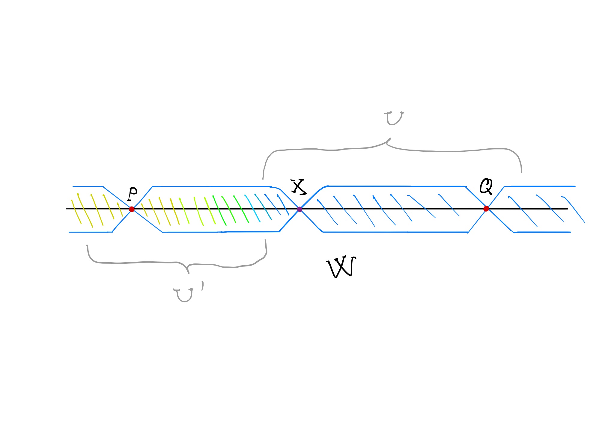
We first discuss the data associated to . It is a coherent choice of perturbations such that restricts to at and to at both and . Moreover, over the cobordism going from to , is a small deformation of . Such exists by the usual construction of coherent perturbations because the base almost complex structure is the same for both and and there are no (non-marked) tear drops. The marking of coincides with that of over and there are no markings over the bottleneck . The purpose of the proof is to show that there is a marking over that consists only of self-intersection points that are action-negative and such that the marking makes unobstructed.
We denote by the self intersection points of viewed in the fibre over the bottleneck , . We let be the vector space of basis the elements of and consider the element given by . Here is the moduli space of -marked tear-drops with boundary on , defined with respect to the data and with output at . As is the marking over , all these tear-drops have marked inputs over . Of course, are only counted (with coefficients in ) the elements in those moduli spaces that are dimensional. By taking the deformation sufficiently close to and considering the action inequalities as in Remark 3.3.3 c, we see that whenever is not void the point is action negative. We now define to be the union of all the self-intersection points that appear in and . Because is a sufficiently small deformation of the identity over the segment from to , we deduce that at each point the number of marked tear drops is now , as the number of tear-drops coming from agrees with the number (mod ) of tear-drops coming from (see also the proof of Lemma 3.4.2). It follows that is unobstructed and this concludes the proof. ∎
4.2.2. Cabling and counting tear-drops.
In this section we revisit the cabling construction from §2.1.3 with the aim to show:
Proposition 4.2.12.
Along the way towards proving this result we will also need to adjust the cabling construction to our setting, in a way that takes into account the deformations of the immersed cobordisms and .
Proof.
Using Lemma 4.2.1 we see that it is sufficient to show that and are cabling equivalent iff where is a small enough deformation of for an appropriate curve . There are three steps to show this.
Step 1. Cabling taking into account markings and perturbations.
We now consider two cobordisms . We define the cabling of and , , by revisiting the construction in §2.1.3 and, in particular, Figure 11. We consider the Lagrangian represented in Figure 46 below (the components, and , appear in Figure 10). To fix ideas, we will first assume that and that and intersect transversely.
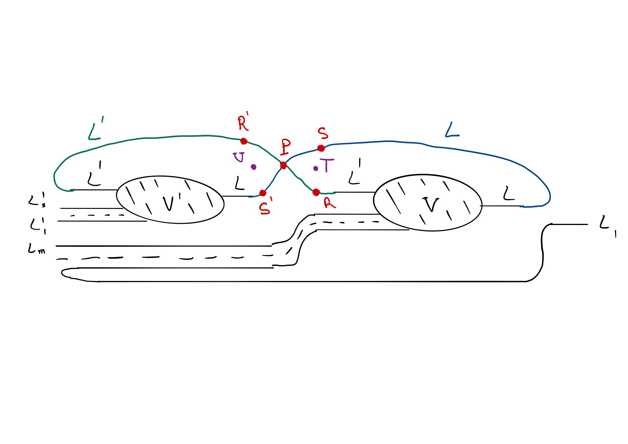
We now list details of the construction. The data for is and for it is and we have the two primitives and (that are viewed as defined on and ).
- i.
The bottlenecks and are associated to the respective ends of and, respectively, with the structure induced from the deformed cobordisms and .
- ii.
Postponing for the moment discussion of the relevant perturbation data, the segments , , and respectively , , represent sufficiently small deformations of products of the form and, respectively, with the respective segment along the curves in green and blue in Figure 46.
- iii.
The profile of the gluing at for each of the two branches, one associated to - with a restriction at written as and the other associated to , with restriction at written as , is as in Figure 36.
- iv.
The points and are pivots associated to .
- v.
The primitives and are extended to a primitive (this is defined on the domain of the immersion and the “sizes” of the blue and green curves in Figure 46 might need to be adjusted to ensure the existence of the primitive ). The restriction of to the submanifold is denoted and similarly for the restriction to which is denoted by . The curves in blue and green in Figure 46 are picked in such a way that .
We further discuss the markings and data associated to the cabling . To proceed, we first fix the perturbation data associated to the ends we are interested in. Thus the data for is and that for is . A key point here is that for the perturbation data for the cabling to make sense it has to be chosen in a coherent way for both and for when viewed as Lagrangians . To achieve this we will make use of Lemma 4.2.11. We first pick perturbation data that is coherent (and unobstructed) for both and . By Lemma 4.2.11, there are unobstructed cobordisms from to and similarly from to . Here , are markings determined as in Lemma 4.2.11. We pick the perturbations in question here so that the cobordisms and are defined (see Corollary 4.2.9).
With these cobordisms , given with the associated perturbation data, the additional conditions on the cabling are as follows:
- vi.
The data of restricted to , viewed from a neighbourhood of and to a neighbourhood of coincides with the data of , including the markings. Similarly, the data of restricted to viewed from a neighbourhood of to a neighbourhood of coincides with the data of .
- vii.
The cobordism together with its perturbation data restricts to along the segment and to the cobordism along . Similarly, restricts to along and to along .
- viii.
The marking of contains the marking and for and as described at point vi, the markings and over together with a set (possibly void) of new points of the form where such that .
- ix.
The pivots of are the union of the pivots of and and of and . Finally, the data for is coherent and regular also with respect to the pivots .
Two cobordisms are, by definition, cabling equivalent if there exists a cobordism , with a choice of coherent perturbation data as described above, such that is unobstructed.
Step 2. Tear-drops and the classes .
The purpose of this paragraph is to show that the homology class (from Lemma 4.2.1) can be determined by counting the tear-drops in Figure 46 with output at and with one interior marked point that is sent to . More precisely, let be the moduli space of marked tear-drops with one interior marked point sent to and output at the point . Notice that the condition on the interior marked point implies that the marking of the potential entries of such a tear-drop are only at points in . Consider the element (again the count is only for those moduli spaces of dimension ). We want to notice that is a cycle and that is identified (in a precise sense to be made explicit) with . We will make use of Figure 47 below.

In this figure appears a sufficiently small perturbation of . This has again three regular bottlenecks at the points , and (as well as two inverted bottlenecks that are no longer pictured). By considering the -dimensional moduli spaces of the form and their boundary, it is easy to see that is indeed a cycle. We then consider the -dimensional moduli space of marked Floer strips with one interior marked point (again sent to ) that have an input at the point and with output at and with the part of the boundary along and the part of their boundary along . From the structure of the boundary of this moduli space we see that there are two maps and that are chain homotopic. Here is the chain map given by the marked Floer strips (with one interior marked point that is sent to ) that exit the point and enter in . The operation is given by (marked) triangles with entries at and at and output at . As is a small deformation of and is the composition of two inverse cobordisms over the interval it follows that is chain homotopic to the identity. We now apply and to the unit viewed in the (marked) Floer complex in the fiber over . We obtain . This means that where is the isomorphism between the complexes and induced by the cobordism restricted to the segment , changing the data to (as described in Lemma 4.2.11).
Denote now by the cycle defined by counting marked tear-drops with an interior marked point being sent to (see Figure 46). It follows, from an argument similar to the one above, that where is the identification using (the restriction of to) the interval .
Step 3. Conclusion of the proof.
We start by remarking that the construction of the cabling at Step 1, together with the coherent, regular perturbation data and the marking is possible by the usual scheme. It is useful to note here that, as we are only using tear-drops with interior marked points we may pick coherent perturbations inductively, following the total valence of the curves involved. In particular, the cycles , are well defined as in Step 2. Notice that these cycles do not depend on the part of the marking given by self-intersection points of that belong to . We denote this part of the marking by .
We now want to remark that there is a choice of making unobstructed if and only if . This shows the statement as it implies, by Step 2, that if an only if and are cabling equivalent.
In turn, the cobordism (together with the data defined before) is unobstructed if and only if for any self intersection point the number (mod ) of marked tear-drops with output at is . Given that both and are unobstructed and in view of the presence of the bottleneck at the point , the only points where the number of tear-drops might not vanish are the points . We now consider such a point and the moduli spaces of tear-drops that have as an output. A marked tear-drop with output at has a projection onto the plane that is holomorphic in a neighbourhood of . As a result this tear-drop could be either completely contained in , or if its projection onto the plane is not constant, then the image of is either to the left or to the right of since otherwise the image of the curve would enter one of the unbounded quadrants at the point . Moreover, is simple in a neighbourhood of . This is seen as follows. First, because is a marked teardrop and in view of the action condition on the points belonging to the marking, none of the entry puncture points of can belong to as otherwise the image of would again intersect one of the unbounded quadrants at (if an output lies over , then the curve will “get out” of through one of the unbounded quadrants). Secondly, due to asymptotic convergence at the exit boundary point, the restriction of to some neighbourhood of the exit puncture is simple and, again because the image of can not intersect one of the unbounded quadrants at , it follows that is simple over a possibly smaller neighbourhood of the exit. Thus, we deduce that is simple in a neighbourhood of .
We conclude that either is constant equal to or belongs to one of or . Denote by the set of tear-drops with a constant projection. Here is the marking . Notice that we can write where is the differential of the Floer complex . Of course, we work here - as before - with the Floer complex with a differential counting marked strips, with the marking for and for . We conclude therefore that the total number (mod ) of marked tear-drops at the point is . Unobstructedness of is equivalent to the vanishing of all these numbers and thus to the equality . This means that if is unobstructed, then . Conversely, if we can pick to be such that and then the cabling defined as above and with is unobstructed. ∎
Remark 4.2.13.
a. The fact that we work over is important in these calculations. It is clear that to work over one needs not only to fix spin structures (so that the various moduli spaces are oriented) but also to allow -size surgery with weights (essentially allowing integral multiples of the same intersection point).
4.3. From algebra to geometry.
4.3.1. Surgery over cycles and geometrization of module morphisms.
The main purpose of this subsection is to show that Axiom 4 from §2.2 is satisfied in our context. In other words, we need to show that for any morphism there exists a surgery morphism that is cabling equivalent to . By Proposition 4.2.12 this is equivalent to finding such that . This property is a consequence of the next result.
Proposition 4.3.1.
Let and let be a cycle. Then there exists a marked cobordism , such that
Proof.
It is not hard to construct a cobordism with double points containing -dimensional clean intersections, that represents the trace of a -size surgery: we can simply put where , are the curves from Figure 48 (see also §2.1.2) this cobordism has three ends (indicated here with their markings): , and . The difficulty is to construct a deformation of this together with the associated marking of so that this marking restricts to the markings of the ends (as in Definition 3.2.2) and such that is unobstructed, so that, together with the relevant perturbation data, we get an element in .
We start with the two Lagrangians and viewed as elements in and thus endowed with the additional data , . Additionally, the primitives and are also fixed. In view of Corollary 4.2.9 and Lemma 4.2.11 we may assume that and are intersecting transversely at points different from the self-intersection points of both and and that there is a choice of coherent data associated to the immersed Lagrangian that extends both and . To fix ideas, we indicate from the start that the cobordism that we will construct will consist of the union of two sufficiently small deformations of and of , with and two curves to be described below in Figure 48, together with additional marking points associated to . In other words is a Lagrangian immersion with domain the disjoint union and . The primitive on restricts to on the factor and to on the factor.
Notice that the curves , themselves are tangent at the point and they coincide along the bottom leg in the picture, to the left of . The points , , and are regular bottlenecks and there are inverted bottlenecks . The primitives and restrict to the primitives at and at and, by possibly having make an “upper bump” in between and we may assume that the primitive restricts at along to a primitive on , , such that where is the corresponding restriction of .
There are four “regimes” governing the perturbations providing and we describe them now. Denote by small disks around the self-intersection points of , let be small disks around the self-intersections points of (in each case we view an intersection point as a pair and similarly for ). Let also , be small disks around the intersection points of with , . The first regime is non-perturbed: one portion of , is given as:
The second portion contains a perturbation around the self intersection points of in the sense of the small perturbation of the cobordism as in §3.4.4. In other words, if are two disks with , , , then
Similarly, there is another portion that corresponds to a similar small perturbation of .
Finally, there is yet one other portion, , which is given in terms of the disks , by:

These four parts of are glued together by using perturbations on slighter larger disks such that (and similarly for , and ). This is possible because the curves , are Hamiltonian isotopic in the plane to (and similarly for the curves). This Hamiltonian isotopy can be lifted to and the gluing uses an interpolation between this Hamiltonian defined on and the trivial one defined on exterior of .
The next point is to discuss the marking of and the relevant data . The markings appear at the points where it is given by , at where it is given by , at where it is given by and at where it is again . Notice that this makes sense as consists of pairs such that . It follows that for the pairs as above we have (when all the relevant perturbations are sufficiently small). The data restricts to the data in neighbourhoods of the four regular bottlenecks . Away from the bottlenecks the data is a small deformation of . The deformations giving , as well as are taken sufficiently small such that with this data both and are unobstructed. Notice that is a deformation of the immersed cobordism , as desired.
We now want to show that, after possibly diminishing these perturbations even more, (which is viewed as the end over the bottleneck ) is unobstructed and that the cobordism is also unobstructed. We start with . Because both and are unobstructed, it is immediate to see that the only marked tear-drops with boundary on and that are not purely on or on , have to have some marked inputs . Moreover, because the markings are action negative and because we also have the same type of inequality at . This implies that a marked tear-drop with boundary on can have at most one marked point as an input (to have more such points, the boundary of the tear-drop should cross back from to at some other input but that input can not belong to due to the action inequality). In this case, obviously, the output is some intersection point . We now consider the moduli space of such teardrops at , . It is immediate to see that this moduli space can be written as a union where are precisely the markings for and for . In other words, is the moduli space of marked Floer strips with boundaries on and , originating at and ending at . Considering now only the -dimensional such moduli spaces and recalling that the data ensures regularity, we have
because, by hypothesis, is a cycle (here is the (marked) Floer differential). Therefore, we conclude that is unobstructed.
We pursue by analyzing . We again start by using the fact that and are each unobstructed. Therefore, the only type of tear-drops with boundary on that we need to worry about are those having a marked input or and output in . But we may assume that the cobordism restricted to the region in between and is in fact a sufficiently small deformation of where is the part of in between and (it agrees there with ). This implies that that this region of is also unobstructed (by Lemma 3.4.2) and shows that itself is unobstructed.
To conclude the proof of the proposition we still need to show that . For this argument we will use Figure 49 and notice that, by considering a sufficiently small deformation of (as in the figure) and the corresponding data, the morphism is given by counting marked strips from to in Figure 49.

There has to be only one such marking passing from to and the only possibility for such a marking is at the point . Thus this marking has to belong to . In other words, we have where is the multiplication for the following three Lagrangian cobordisms given by counting triangles such a in the Figure. It is not difficult to see that is the unit (in homology) for this multiplication and thus which concludes the proof.
∎
4.3.2. has surgery models.
In this subsection we intend to finish showing that the category satisfies the Axioms from §2.2. Given that we already constructed the functor from Theorem 4.1.1 and that we showed in Proposition 4.2.12 that and are cabbling equivalent iff , we already know that the quotient functor is well defined and injective. It follows that Axioms 1 and 2 are satisfied. We showed in §4.3.1 that Axiom 4 is also satisfied.
It remains show that Axiom 3, which was verified for elements in in Corollary 4.2.9, is also true for general ’s . Moreover, we need to show that the functor is triangulated. Indeed, if this is so, Axiom 5 - in the form made explicit in Remark 2.3.3 b - is also satisfied because the relevant naturality properties are already satisfied in the triangulated category which is the image of the injective functor .
Therefore, taken together, these two claims imply that has surgery models.
Lemma 4.3.2.
If is a simple cobordism , possibly carrying (non marked) tear-drops, then .
Proof.
Given that may carry tear-drops, we need to deal with the possible presence of pivots. The difficulty that these create is that the argument used in Corollary 4.2.9, which is based on a Hamiltonian isotopy induced by a translation in the plane, is no longer directly applicable as the image of the moving cobordism intersects the pivots. The argument makes use of Figure 50 below. The ends of the cobordism are and . We consider a Lagrangian , , where is a circle intersecting the cylindrical region of at the point and and is in in generic position relative to and . For the moment, we assume is embedded. The points and are regular bottlenecks for .
Following the definition of (see equation (19)) we see that this morphism is given by counting (marked strips) going from points to points where , . Similarly, is given by counting the strips going from to . We now consider the composition and view it as providing a count of the points in a part of the boundary of the moduli space of marked strips going from to . Another such part consists of disks of Maslov class with boundary on , going through the points in . If the deformations giving out of are sufficiently small, we see that there is precisely one such disk for each point in and we conclude that is chain homotopic to the identity. The same argument actually shows that the composition is chain homotopic to the identity as an -module map and concludes the proof (alternatively, we apply the same geometric argument as before to the case when is no longer embedded and is a small enough deformation of ). ∎
Lemma 4.3.3.
The functor is triangulated.
Proof.
Recall from §2.1.1 and Figure 4 the definition of the distinguished triangles in . It is easy to see that the distinguished triangle associated to a surgery cobordism , such as constructed in §4.3.1, is mapped by to an exact triangle in the homological category of -modules over (a simple proof in this case is perfectly similar to the embedded case in [BC2]). However, we need to deal with the case of , , when possibly carries (non-marked) tear-drops. To do this we provide a different proof, along an approach similar to the one in Lemma 4.3.2. We consider Figure 51 below (compare with Figure 50). There are now three regular bottlenecks , each corresponding to one of the ends of . The curve is a circle, as in Figure 50. We consider a Lagrangian where is embedded, in generic position relative to all three of .
We again consider the (marked) Floer complex generated by the points and similarly , for the other ends of . There is a chain map that we denote by (and, similarly, , ) defined by counting Floer (marked) strips going from intersection points over to intersection points over . These three maps are respectively identified with the three maps associated through the construction of to the three maps in the distinguished triangle corresponding to , as given in Figure 4. Thus we need to show that these three maps fit into an exact triangle of chain complexes (and, by extension, of -modules). For this purpose, denote by the cone of the map : it is given as vector space by and has the differential . There is a chain map defined by counting strips from intersection points over either or to intersection points over . Moreover, there is a chain map given by counting strips from intersection points over to intersection points that are either over or . As in the proof of Lemma 4.3.2 these two maps are homotopy inverses. We notice that the projection composed with agrees with and that composed with the inclusion agrees with which shows that the three maps , , fit into an exact triangle in the homotopy category.
∎
4.4. Proof of Theorem 4.1.1
Most of Theorem 4.1.1 has been already established. We need to only discuss here the metric statements in this theorem.
We start by defining the shadow of an element . Recall that has regular bottlenecks along each of its ends and let be the part of that is left after removing the regions to the left of the positive bottlenecks and to the right of the negative bottlenecks, as in Figure 52 (compare with the cobordism from Figure 40). The shadow of is by definition, the shadow of , in the sense of §2.4.
Notice that the band width parameter, , appearing in the definition of the perturbation germs associated to an element , as discussed in §3.4.1, can be taken arbitrarily small. Making use of this and noticing also that in the construction of the surgery morphisms in §4.3 we may take the various relevant deformations with an arbitrary small area covered by their shadows - this applies to as well as the deformations giving the cobordisms and - we deduce that the category has small surgery models in the sense of §2.4.
The next step is to see that satisfies the rigidity Axiom 6 from §2.4. We will prove the stronger fact that is strongly rigid.
Lemma 4.4.1.
The category is strongly rigid (see Definition 2.4.1).
Proof.
The first part of the proof is to show that is rigid. This means that we need to show that for any two different Lagrangians there exists a constant such that for any simple cobordism , we have .
Recall that for two Lagrangians and , the Gromov width of relative to is defined by
where is a symplectic embedding, is the standard ball of radius and .
Assume now that , is a simple cobordism. Proceeding as in [CS] we deduce that through the center of a ball as in the definition of , passes a perturbed marked -holomorphic strip with boundary along and on and of energy not bigger than .
The energy of is bounded from below by the energy of . By adjusting the data associated to the pair , there exists a constant depending of the perturbations and (and thus also of the base almost complex structure ) such that the energy of is bounded from below by (if the almost complex structure used inside could be assumed to be the standard one and the perturbations vanish there, the energy in question would agree with the symplectic area and we could take ).
In summary, we have
| (21) |
which implies that Axiom 6 is satisfied at least for simple cobordisms that do not carry non-marked tear-drops. In case , the argument in [CS] no longer applies because the argument there is based on a Hamiltonian isotopy such as the one appearing in Lemma 4.2.7 and this isotopy potentially intersects the poles associated to . However, a quantitative adjustment of the argument in Lemma 4.3.2 does imply the statement even in this case.
Consider now a cobordism , . Using the braiding in Remark 2.3.2, we may replace it by a cobordism where is obtained by iterated -size surgeries involving the ’s and . Because has small surgergy models, the cabling used in the braiding can be assumed to add to the shadow of the initial cobordism as little as wanted. In short, for any we can find such a so that . Assume now that there are families and with totally discrete and such that . Focusing for now just on the family , it follows from the arguments above that, for any , there is a cobordism of shadow less than with . Consider now a point . As there exists a sufficiently small standard symplectic ball around (as in the definition of width) that also does not intersect , we deduce from (21) that . There is a small open set containing and thus we deduce that all of . We apply the same argument to and we arrive at a contradiction because of our assumption on and . ∎
To conclude the proof of Theorem 4.1.1 there are two more statements to justify. The most important part is that the restriction of the morphism to the triangulated subcategory generated by the embedded Lagrangians gives a triangulated isomorphism to . The functor is triangulated and all modules in are iterated cones of Yoneda modules of embedded objects. Therefore, by using Proposition 4.3.1, recurrence on the number of cones and equation (16) the result follows. Notice also that it also follows from Proposition 4.3.1 and equation (16) that the category itself is the Donaldson category associated to the Lagrangians in .
Remark 4.4.2.
Notice that in this construction the base almost complex structure that one starts with can be any almost complex structure on because exact, embedded Lagrangians are unobstructed with respect to any such structure. Moreover, because we use in Proposition 4.3.1 -size surgeries, all modules in are represented by marked immersed Lagrangians so that the immersion restricts to embeddings on the connected components of . In other words, in order to represent the only immersions required are unions of embedded Lagrangians together with appropriate choices of markings that are used to deform the usual Floer differential as well as the higher multiplications.
5. Some further remarks.
5.1. Related results.
As mentioned before, the literature concerning Lagrangian cobordism starts with the work of Arnold [Arn1], [Arn2] who introduced the notion. Rigid behaviour first appears in this context in a remarkable paper due to Chekanov [Che]. All the consequences and particular statements that result from the existence of the functor in §4.2.1, when applied to only embedded Lagrangians and cobordisms, were established, mainly in [BC1] and [BC2]. A variety of additional facts are known and, as they also contribute to various other aspects of the geometry - algebra dictionary discussed here, we will rapidly review the relevant literature here.
5.1.1. Simple cobordisms.
As discussed before, unobstructed simple cobordisms are inducing isomorphisms between the Floer theoretic invariants of the two ends. More is likely to be true: for instance simple exact cobordisms are conjectured to coincide with Lagrangian suspensions. Steps towards proving this conjecture are due to Suarez [SL] and Barraud-Suarez [BS]. They prove, under constraints on the behaviour of the fundamental group inclusions of the ends, that an exact simple cobordism is a pseudo-isotopy (in other words, the cobordism is smoothly trivial).
5.1.2. Additional algebraic structures.
There are a variety of results of this sort. Among them: relations with Calabi-Yau structures due to Campling [Cam]; to stability conditions, discovered by Hensel [Hen]; can be used [CC] to provide a categorification of Seidel’s representation that views this representation as an algebraic translation of Lagrangian suspension; cobordisms can be studied also in the total space of Lefschetz fibrations over the complex plane [BC3]; they also can be used to approach from a different angle a Seidel type exact sequence for generalized Dehn twists [MW]. Some connections to mirror symmetry appear in Smith-Sheridan [SS].
5.1.3. Cobordism groups.
Following earlier results due to Audin [Aud] and Eliashberg [Eli] that compute in the flexible case cobordism groups in euclidean spaces by means of algebraic topology, there are essentially two recent calculations in the rigid case. Both apply to surfaces: Haug [Hau] for the torus and Perrier [Per1] (this last paper contains a number of gaps and errors, a corrected version is in preparation by Rathel-Fourrier [RF]) for surfaces of genus at least two.
5.1.4. Variants of the “surgery models” formalism.
It is likely that the concept of a cobordism category with surgery models, or a variant, can be applied to some other contexts. There is some work in progress of Fontaine [Fon] who studies a related formalism for Morse functions. In a different direction, it is not clear for now whether the five axioms governing categories with surgery models in the paper are in any way optimal.
5.1.5. Measurements and shadows.
As mentioned earlier in the paper, shadows of cobordisms have first appeared in [CS] for the case of simple cobordisms and in the wider setting of general cobordisms in [BCS] where are also introduced fragmentation metrics. A variety of interesting related results are due to Bisgaard [Bis2], [Bis1]. In a different direction, an interesting new approach is due to Chassé [Cha] who is exploring the behaviour of shadow type metrics for classes of Lagrangians under uniform curvature bounds.
5.1.6. Other approaches/points of view.
Lagrangian cobordism has also been considered from a different perspective by Nadler-Tanaka [NT], [Tan]. There are connections, only superficially explored at the moment, to micro-local sheaf theoretic techniques as evidenced in work of Viterbo [Vit] (page 55).
Finally, there is considerable work today on cobordisms between Lagrangians through Legendrians. This is certainly a different point of view relative to the one that is central to this paper but there are also a variety of common aspects. For remarkable applications of this point of view see Chantraine-Rizell-Ghiggini-Golovko [CRGG].
5.2. Some further questions
5.2.1. Non-marked Lagrangians.
As mentioned before in the paper, in general, rigid cobordism categories with surgery models have to contain immersed Lagrangians among their objects. A natural question is whether one can have objects that are non-marked (or, in other words, with the empty markings).
In some framework the answer to this question is expected to be in the affirmative (thus providing a non-tautological solution to Kontsevich’s conjecture). However, there are some difficulties in achieving this, some conceptual and some technical.
Here are two examples of the problems on the conceptual side.
- a.
The -surgery at some intersection points with and , exact is only exact (with suitable choices of handles) if is the same for all . As a result, the morphisms that can be obtained through an analogue of Proposition 4.3.1 are associated to cycles of intersection points that have the same action. On the other hand there is no such control of the action of the points representing with the functor in §4.2.1 and thus it is not clear whether all the image of , at least as defined in §4.2.1, can be represented geometrically.
- b.
we have not discussed here changing the base almost complex structure but it is certain that such changes in any case lead to a set-up involving bounding chains.
The technical difficulties involved to remove from the picture marked Lagrangians and replace them with immersed but non-marked ones, already appear at the following point. We need to compare for varying and fixed and for and embedded. Assuming the marked Lagrangian is unobstructed (in the marked sense), the basic questions are whether it is true that:
- i.
The non-marked Lagrangian is also unobstructed.
- ii.
The surgery cobordism from to for small enough is also unobstructed and the relevant Yoneda modules of and are quasi-isomorphic.
A key step is to compare moduli spaces of marked tear-drops with boundary on to the moduli spaces of non-marked tear-drops with boundary on , after rounding the corners at the marking , as pictured in Figure 53 (assuming the dimension of these moduli spaces is ). The two moduli spaces need to be identified for small. While intuitively clear, this identification is not obvious. It depends on a gluing result that appears in [FOOO1] but, beyond that, there are other subtleties. For instance, to ensure regularity of it is natural to use non-autonomous almost complex structures. On the other hand consists, by default, of autonomous complex structures, thus these moduli spaces are not so easy to render regular. Additionally, the gluing result in [FOOO1] applies to autonomous curves. Regularity of curves defined with respect to autonomous structures and without perturbations can potentially be approached as in [Laz], as attempted in [Per2] (but this paper is not complete at this time).
Further, the same methods need also to be applied to deal with moduli spaces of -holomorphic disks and with more complicated curves. This requires a more general gluing statement of the type of the one in [FOOO1], that applies to polygons with more than a single corner having boundary on a generically immersed Lagrangian submanifold. Moreover, one also needs a version of the Gromov compactness theorem that applies to curves with boundary on a sequence of Lagrangians that converges to an immersed Lagrangian through a process that corresponds to reducing to zero the size of a handle attached through surgery.
An additional issue, related to the application of the Gromov compactness argument in this setting, is that to achieve the comparison between the moduli spaces and one needs uniform energy bounds that apply for all -surgeries for small enough. Otherwise, the moduli spaces might contain curves with energy going to when and these curves obviously are not “seen” by the spaces .
5.2.2. Bounding chains and invariance properties.
As mentioned before in §1.3.3, bounding chains and the markings of Lagrangian immersions used in this paper are closely related. Recalling from [AJ] the Akaho-Joyce algebra associated to an immersed Lagrangian , it is easy to see that a marking associated to provides a bounding chain for this algebra. Moreover, the marked Flower homology of two such marked Lagrangians and is the corresponding Floer homology associated to the respective bounding chains. Conversely, possibly under some additional conditions, it is expected that a bounding chain can be reduced to a marking.
Exploring in more detail the relation between markings and bounding chains is also of interest because the notion of unobstructedness used in the paper is somewhat unsatisfying as it depends on a specific choice of a base almost complex structure . Certainly, it remains true that the resulting category is a model for the derived Fukaya category of the embedded objects and thus it does not depend of up to triangulated isomorphism. Nonetheless, it is expected that a more invariant construction would make explicit use of bounding chains to adjust the markings, data etc when transitioning from one base almost complex structure to another.
In this context, an interesting related question is to understand the behaviour of bounding chains with respect to surgery. A first step in this direction appears in [PW].
5.2.3. Novikov coefficients.
Going beyond -coefficients seems possible and, in particular, using coefficients in the universal Novikov field. This extension is however not completely immediate as it requires using surgery with coefficients that take into account the size of the handles. In other words, where in the body of the paper we viewed surgery as an operation associated to a cycle where now we need to consider cycles of the form with and the surgery needs to take into account the size of the ’s.
5.2.4. Idempotents.
With motivation in questions coming from mirror symmetry it is natural to try to understand how to take into account idempotents in the global picture of the cobordism categories considered here. This turns out not to be difficult (even if we leave the details for a subsequent publication): one can view idempotents as an additional structure given by a class in the quantum homology defined for each one of the ends of a cobordism and such that . A similar structure also makes sense for a cobordism , in this case the relevant class belongs to . There is a connectant and the requirement for a cobordism respecting the idempotents is for the classes on the boundary to descend from that on . The case of standard cobordisms is recovered when all these classes are the units. For embedded Lagrangians, the additional structure provided by idempotents is not hard to control (compared to what was discussed before one also needs to show that the various morphisms induced by cobordisms also relate in the appropriate way the idempotents of the ends). However, we expect that the whole construction will be of increased interest when cobordisms and their ends are allowed to be immersed. The second author thanks Mohammed Abouzaid for a useful discussion on this topic.
5.2.5. Small scale metric structure.
For an embedded Lagrangian , a basic question is whether there is some such that, if for some , then is also embedded and, further, is Hamiltonian isotopic to . Could it be that even more is true for possibly even smaller: there is a constant only depending on such that (where is the Hofer distance) ?
5.2.6. Embedded vs. immersed.
There are two natural questions related to the formalism discussed here. Are there criteria that identify objects of that are not representable by embedded Lagrangians? Similarly, are there criteria that identify un obstructed immersed, marked, Lagrangians that are not isomorphic to objects of ?
References
- [AB1] G. Alston and E. Bao. Immersed lagrangian floer cohomology via pearly trajectories. Preprint (2019). Can be found at https://arxiv.org/abs/1907.03072.
- [AB2] G. Alston and E. Bao. Exact, graded, immersed lagrangians and floer theory. J. Symplectic Geom., 16(2):357–438, 2018.
- [AJ] M. Akaho and D. Joyce. Immersed lagrangian floer theory. J. Differential Geom., 86(3), 2010.
- [Aka] M. Akaho. Intersection theory for lagrangian immersions. 12(4):543–550, 2005.
- [Arn1] V. Arnol′d. Lagrange and Legendre cobordisms. I. Funktsional. Anal. i Prilozhen., 14(3):1–13, 96, 1980.
- [Arn2] V. Arnol′d. Lagrange and Legendre cobordisms. II. Funktsional. Anal. i Prilozhen., 14(4):8–17, 95, 1980.
- [Aud] M. Audin. Quelques calculs en cobordisme lagrangien. Ann. Inst. Fourier (Grenoble), 35(3):159–194, 1985.
- [BC1] P. Biran and O. Cornea. Lagrangian cobordism. I. J. Amer. Math. Soc., 26(2):295–340, 2013.
- [BC2] P. Biran and O. Cornea. Lagrangian cobordism and Fukaya categories. Geom. Funct. Anal., 24(6):1731–1830, 2014.
- [BC3] P. Biran and O. Cornea. Cone-decompositions of Lagrangian cobordisms in Lefschetz fibrations. Selecta Math. (N.S.), 23(4):2635–2704, 2017.
- [BCS] P. Biran, O. Cornea, and E. Shelukhin. Lagrangian shadows and triangulated categories. Preprint (2018). Can be found at http://arxiv.org/pdf/1806.06630v1.
- [BEH+] F. Bourgeois, Y. Eliashberg, H. Hofer, K. Wysocki, and E. Zehnder. Compactness results in symplectic field theory. Geom. Topol., 7:799–888, 2003.
- [Bis1] M. R. Bisgaard. A distance expanding flow on exact Lagrangian cobordism classes. Preprint 2016, Can be found at arXiv:1608.05821 [math.SG].
- [Bis2] M. R. Bisgaard. Invariants of Lagrangian cobordisms via spectral numbers. Preprint 2016, Can be found at arXiv:1605.06144 [math.SG].
- [BS] J.-F. Barraud and L.S. Suarez. The fundamental group of a rigid lagrangian cobordism. Annales Math. du Quèbec, 43:125–144, 2019.
- [Cam] E. Campling. Fukaya categories of lagrangian cobordisms and duality. Preprint, can be found at arXiv:1902.00930 [math.SG].
- [CC] F. Charette and O. Cornea. Categorification of Seidel’s representation. Preprint (2013). To appear in Israel Journal of Math. Can be found at http://arxiv.org/pdf/1307.7235v2.
- [Cha] J.-P. Chassé. PhD Thesis, University of Montreal, in progress. PhD thesis.
- [Che] Y. Chekanov. Lagrangian embeddings and Lagrangian cobordism. In Topics in singularity theory, volume 180 of Amer. Math. Soc. Transl. Ser. 2, pages 13–23. Amer. Math. Soc., Providence, RI, 1997.
- [CL] O. Cornea and F. Lalonde. Cluster homology: an overview of the construction and results. Electron. Res. Announc. Amer. Math. Soc., 12:1–12, 2006.
- [CRGG] B. Chantraine, G. D. Rizell, P. Ghiggini, and R. Golovko. Geometric generation of the wrapped fukaya category of weinstein manifolds and sectors. Preprint, can be found at arXiv:1712.09126 [math.SG].
- [CS] O. Cornea and E. Shelukhin. Lagrangian cobordism and metric invariants. J. Diff. Geom., 112:1–45, 2019.
- [Eli] Y. Eliashberg. Cobordisme des solutions de relations différentielles. In South Rhone seminar on geometry, I (Lyon, 1983), Travaux en Cours, pages 17–31. Hermann, Paris, 1984.
- [Flo] A. Floer. Morse theory for Lagrangian intersections. J. Differential Geom., 28(3):513–547, 1988.
- [Fon] P. Fontaine. MA Thesis, University of Montreal, in progress.
- [FOOO1] K. Fukaya, Y.-G. Oh, H. Ohta, and K. Ono. Lagrangian intersection Floer theory - anomaly and obstruction, chapter 10. Preprint, can be found at http://www.math.kyoto-u.ac.jp/~fukaya/Chapter10071117.pdf.
- [FOOO2] K. Fukaya, Y.-G. Oh, H. Ohta, and K. Ono. Lagrangian intersection Floer theory: anomaly and obstruction. Part I, volume 46 of AMS/IP Studies in Advanced Mathematics. American Mathematical Society, Providence, RI, 2009.
- [Fuk] K. Fukaya. Unobstructed immersed lagrangian correspondence and filtered a infinity functor. Preprint, can be found at arXiv:1706.02131 [math.SG].
- [Hau] L. Haug. The lagrangian cobordism group of . Selecta Math. (N.S.), 21:1021–1069, 2015.
- [Hen] F. Hensel. Stability conditions and lagrangian cobordisms. Preprint, can be found at arXiv:1712.02252 [math.SG].
- [Laz] L. Lazzarini. Relative frames on J-holomorphic curves. Fixed Point Theory and Applications, 9(2):213–256, 2011.
- [LS] F. Lalonde and J.-C. Sikorav. Sous-variétés Lagrangiennes et Lagrangiennes exactes des fibrés cotangents. Comment. Math. Helv., 66(1):18–33, 1991.
- [MW] C.-Y. Mak and W. Wu. Dehn twists exact sequences through Lagrangian cobordism. Preprint (2015). Can be found at http://arxiv.org/pdf/1509.08028.
- [NT] D. Nadler and H.L. Tanaka. A stable infinity-category of lagrangian cobordisms. Preprint (2011). Can be found at http://arxiv.org/pdf/1109.4835v1.
- [Per1] A. Perrier. Lagrangian cobordism groups of higher genus surfaces. Preprint, can be found at arXiv:1901.06002 [math.SG].
- [Per2] A. Perrier. Structure of J-holomorphic disks with immersed Lagrangian boundary conditions. Preprint, can be found at arXiv:1808.01849 [math.SG].
- [Pol] L. Polterovich. The surgery of Lagrange submanifolds. Geom. Funct. Anal., 1(2):198–210, 1991.
- [PW] J. Palmer and C. Woodward. Invariance of immersed Floer cohomology under Lagrangian surgery. Preprint, can be found at arXiv:1903.01943v1 [math.SG].
- [RF] D. Rathel-Fourrier. PhD Thesis, University of Montreal, in progress.
- [Sch] F. Schmäschke. Floer homology of Lagrnagians in clean intersction. Preprint, can be found at arXiv:1606.05327 [math.SG].
- [Sei] P. Seidel. Fukaya categories and Picard-Lefschetz theory. Zurich Lectures in Advanced Mathematics. European Mathematical Society (EMS), Zürich, 2008.
- [SL] L. S. Suarez-Lopez. Exact Lagrangian cobordism and pseudo-isotopy. 2017.
- [SS] I. Smith and N. Sheridan. Rational equivalence and Lagrangian tori on K3 surfaces. Preprint, can be found at arXiv:1809.03892 [math.SG].
- [Tan] H. Tanaka. Generation for Lagrangian cobordisms in Weinstein manifolds. Preprint, can be found at arXiv:1810.10605 [math.SG].
- [Vit] C. Viterbo. Sheaf quantization of lagrangians and floer cohomology. Preprint, can be found at arXiv:1901.09440 [math.SG].