Randomly Aggregated Least Squares
for Support Recovery

Our idea is quite simple: to estimate ${\mbox{\boldmath$\theta$}}^{*}$, we will use least squares. This naive approach is a bad idea since

tends to require a fairly large number of queries $N$ to recover ${\mbox{\boldmath$\theta$}}^{*}$ stably. The proposed scheme is based on the following observation: instead of running least squares on the full set of equations, we can use only a random subset of the equations. The underlying idea behind RAWLS (Randomly Aggregated Unweighted Least Squares Support Recovery)¹¹ 1 ‘The natural distribution is neither just nor unjust; nor is it unjust that persons are born into society at some particular position. These are simply natural facts. What is just and unjust is the way that institutions deal with these facts.’ (John Rawls, ’A Theory of Justice’ [26]). is that none of the equations are distinguished: taking merely a subset of them amounts to a loss of information but provides a particularly unique point of view. However, since no particular subset of the equations is distinguished over any other subset, we average over a number of randomly selected subsets. Our analysis shows that this is indeed advantageous: while applying least squares using fewer equations leads to errors from the lack of information, these errors cancel (to some degree) when averaged. More precisely, let $A\subset\left\{1,\dots,N\right\}$, we define ${\mbox{\boldmath$X$}}_{A}$ to be the restriction of $X$ onto the rows whose index is in the set $A$ and likewise for ${\mbox{\boldmath$y$}}_{A}$. We then find

We average this result over many subsets $(A_{i})_{i=1}^{m}$ which we assume, for some fixed $n<\min(N,D)$, to be taken uniformly at random from all $n-$element subsets of $\left\{1,2,\dots,N\right\}$ and use this as our estimate for a rescaling of ${\mbox{\boldmath$\theta$}}^{*}$. We hope that

An example (see Fig. 2) is as follows: let us define ${\mbox{\boldmath$\theta$}}\in\mathbb{R}^{64}$ by setting the first $k=16$ entries to be $\pm 1$ (randomly) and the rest to be 0. We take a random Gaussian matrix ${\mbox{\boldmath$X$}}\in\mathbb{R}^{64\times 80}$, take subsets of size $n=58$ equations and average the least-square recovery over $m=100$ random choices of these $58$ equations. We observe that the reconstructed vector is much larger on the actual support than it is off the support; moreover, it correctly identifies the sign of the entry of $\theta$.

Once we go down to a smaller number of equations $N$, something remarkable happens. For simplicity of exposition, we consider the same problem as above (reconstruction of a vector in $D=64$ dimensions) except now we only observe $N=30$ equations and we average over random subsets of these equations of size $n=18$. We emphasize that this quite the extreme setting; we are operating with very little information. This is reflected in the reconstructed vector (see Fig. 3): it is certainly not the case that the largest $k=16$ entries (by absolute value) correspond to the support of $\theta$. However, what we observe in this setting is the largest entry is indeed located on the support of $\theta$: for this particular choice of parameters $(D,N,n)=(64,30,18)$, this happens in $\sim 90\%$ of all cases. This motivated our RAWLS-based peeling algorithm discussed in §3, where we iteratively remove the coordinate corresponding to the largest reconstructed vector. We note that correctly identifying the first coordinate is the most difficult task; after that we have reduced the problem by decreasing the size of the support, one less dimension $D\rightarrow D-1$, and the same number of equations $N$. This is an easier problem.

We can show that this yields provably good results. Before formally stating the result, we will quickly outline its meaning. Instead of trying to recover the vector ${\mbox{\boldmath$\theta$}}^{*}$, we will try to reconstruct its rescaled version $(n/D){\mbox{\boldmath$\theta$}}^{*}$ via an

where $\pi_{A_{i}}$ denotes the projection onto the subspace $A_{i}$ and the $A_{i}$ are, by an abuse of notation, subspaces of size $n$ chosen uniformly at random (subspaces spanned by the rows of $X$ indexed by $A_{i}$). However, we do not have access to ${\mbox{\boldmath$\theta$}}^{*}\in\mathbb{R}^{D}$, we only have access to ${\mbox{\boldmath$y$}}={\mbox{\boldmath$X$}}{\mbox{\boldmath$\theta$}}^{*}+{\mbox{\boldmath$\omega$}}$. Instead of taking a least squares projection of $y$, we will use the least squares projections of ${\mbox{\boldmath$y$}}_{A_{i}}$ for random subsets of the equations in the hope that this approximately recovers ${\mbox{\boldmath$\theta$}}^{*}$

Several remarks are in order.

1. 1.

   The statement is independent of ${\mbox{\boldmath$\theta$}}^{*}$. In particular, there is no underlying assumption about the structure of ${\mbox{\boldmath$\theta$}}^{*}$ (and ${\mbox{\boldmath$\theta$}}^{*}$ need not be sparse). We also observe that the size of ${\mbox{\boldmath$\theta$}}^{*}$ does not appear on the right-hand side. This respects the problem setup where instead of ${\mbox{\boldmath$X$}}{\mbox{\boldmath$\theta$}}^{*}$ we are given the (additive) noisy version ${\mbox{\boldmath$X$}}{\mbox{\boldmath$\theta$}}^{*}+{\mbox{\boldmath$\omega$}}$, where $\omega$ is a standard Gaussian vector ${\omega}_{i}\sim\mathcal{N}(0,1)$.

2. 2.

   In the setting $n\leq N\ll D$ our analysis is accurate down to constants, both quantities on the right-hand side are asymptotically correct (in the sense of having the correct constant, 1, in front) if the scales separate more and more (see Figs. 4, 5 and the Remark in §4.2).

3. 3.

   The randomness in the choice of the $A_{i}$ is not at all necessary. In fact, the proof suggests that one could simply pick completely deterministic subsets of the $N$ equations as long as none of the individual dimensions are featured too prominently and all are represented roughly an equal number of times in the projections. This is also substantiated by numerical evidence. This poses the question of whether there are ‘good’ deterministic choices of subsets or whether there is a natural weight one could assign to the outcome resulting from each subset of equations (some ‘measure of reliability’).

4. 4.

   The result suggests that using a smaller $n$ leads to a smaller error. However, it also leads to a smaller projection. We can compensate for that by inserting the appropriate scaling in our result from which we obtain

   $$\mathbb{E}_{\textnormal{X},{\omega}}~\left\|\underbrace{\frac{1}{m}\frac{D}{n}\sum_{i=1}^{m}\pi_{A_{i}}{\mbox{\boldmath$\theta$}}^{*}}_{\approx{\mbox{\boldmath$\theta$}}^{*}}-\frac{1}{m}\frac{D}{n}\sum_{i=1}^{m}{\mbox{\boldmath$\widehat{\theta}$}}_{A_{i}}\right\|_{\ell^{2}}\lesssim\frac{\sqrt{D}}{\sqrt{N}}+1.$$

   This shows that there is some flexibility in the choice of $n$. In practice we have found that $n=0.6\min(N,D)$ seems to be particularly suited (though not very different from, say, $n=0.5\min(N,D)$). The precise role of $n$ could be an interesting object for further study.

We conclude by showing Theorem 1 in a simple example. As mentioned above, the terms in the upper bound (without the implicit constant and constant 1 instead) correspond to the sharp asymptotic limiting case where $n\leq N\ll D$. We show the case where $D=10000$, $N=100$ and $1\leq n\leq 100$. For each value of $n$, we sample over $m=20$ random subsets of size $n$ of the $N$ equations. As for the vector $\theta$, it does not actually play a role, we chose it to be a Gaussian vector in $\mathbb{R}^{D}$. We observe that the prediction is quite accurate (and the proof explains why this would be the case – various quantities start concentrating tightly around their expectation).

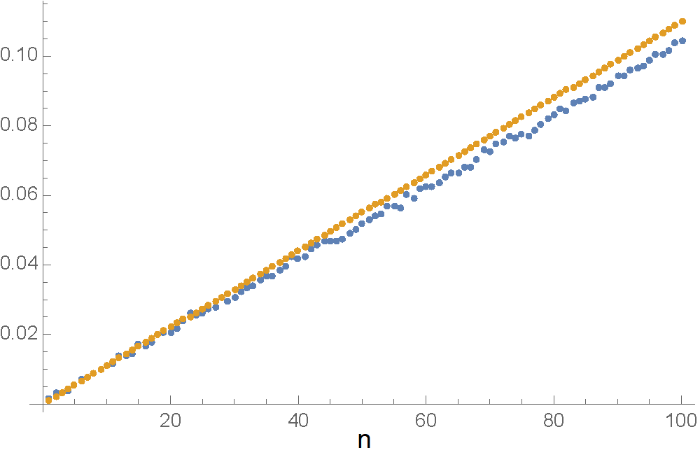
We also quickly illustrate that the restriction $n<0.9\cdot D$ is not just an artifact of the proof but, in fact, necessary (this also explains why RAWLS is better at recovering $\theta$ than an application of least squares to the full set of equations). We consider $\theta$ to be a unit vector (obtained from normalizing an instance of a Gaussian vector) in $D=200$ dimensions. We take $N=200$ equations and see what happens for $1\leq n\leq 195$ (see Figure 5). What we observe is that the theoretical error bound (with the implicit constant assumed to be 1) nicely dominates the error until $n$ starts getting very close to $D$ (we plot it for $1\leq n\leq 195<200=D$). We see that the error starts exceeding the size of the vector by many orders of magnitude. The proof will explain this as a degeneracy of the smallest singular value of a rectangular Gaussian matrix which becomes approximately square.

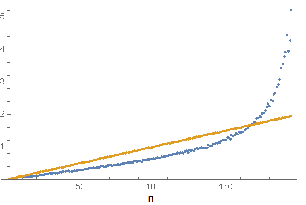
The error observed around $n=195\sim N=D$ demonstrates why least squares using the full set of equations does not work; we obtain similar results also for $N\ll D$, the averaging has a natural stabilizing effect. We refer to the Remark in §4.2. for a prediction for what one would expect the error to look like when, say, $n=0.99D$.

Theorem 1 raises a lot of open questions. Is there a particularly natural choice of subspaces on which to project? We are investigating the case of random projections but the proof does not seem to require this; are there natural ‘adapted’ subspaces that one can derive from a given matrix $X$?
We conclude with a particularly interesting question. We recall that the random projections reduce the size of the resulting vector. We can compensate for that by inserting the appropriate scaling in our result from which we obtain

In the case where we assume $\theta\in\left\{-1,0,1\right\}^{D}$, we want to make sure that we are properly able to distinguish two different vectors of that type and this can then be seen to require $N\sim D$ (not entirely surprising, we are not making any assumptions on the sparsity of $\theta$). However, a more refined approach is conceivable: ultimately, we are using the entries of our approximating vector to derive statements about the support. As such, the $\ell^{2}$ is perhaps not the only interesting quantity and estimates on $\ell^{\infty}$ would be quite desirable. In particular, what we observe in practice (and what motivated the peeling algorithm) is that very large entries (either very large or very small) in the recovered approximation is a good indicator for $\theta$ having support in that coordinate. This simple observations forms the basis of the algorithm discussed in §3. It would be interesting to have results in that direction.

We also emphasize that the idea underlying RAWLS might have many other applications: it is ultimately an $\ell^{2}-$based concept and as such many natural variations seem conceivable. One such applications, a nonlinear variant that is shown to work particularly well in the support recovery problem, is discussed in the next section. A second question, outside the scope of this paper, is whether other methods used for support recovery could conceivably be merged with our philosophy: running it on random subsets of the equations and hoping that the averaging effects compensates for the loss of information.

If it is indeed the case that

and if the error is nicely random (as one usually expects in these cases), then the largest (or smallest) entries of the vector should be contained in the support of ${\mbox{\boldmath$\theta$}}^{*}$. In a more elementary formulation, if we are given ${\mbox{\boldmath$v$}}\in\left\{-1,0,1\right\}^{D}$ (such that $\|{\mbox{\boldmath$v$}}\|_{0}$ is not too small compared to $D$) and add a random Gaussian vector $g$ to it, then the largest (absolute) entry of ${\mbox{\boldmath$v$}}+{\mbox{\boldmath$g$}}$ will be attained (with high probability) on the support of $v$. This is a simple consequence of the rapid decay of the Gaussian, and motivates the Algorithm proposed in the following subsection.

1. 1.

   Compute the approximation

   $${\mbox{\boldmath$\widehat{\theta}$}}=\frac{1}{m}\sum_{i=1}^{m}{\mbox{\boldmath$\widehat{\theta}$}}_{A_{i}},$$

   where $\hat{\theta}$ is estimated based on Eq. 1.

2. 2.

   Find the element of largest absolute value of $\widehat{\theta}$. If this element $\widehat{\theta}_{\ell}$ is positive, then we assume that ${\theta}^{*}_{\ell}=1$; if negative, we assume ${\theta}^{*}_{\ell}=-1$.

3. 3.

   Remove the corresponding column from the matrix $X$ and update the right-hand side $y$ by subtracting the $X$ projected onto the estimated coordinate $\widehat{\theta}_{\ell}$.

4. 4.

   Return to (1) until $k$ non-zero entries of $\widehat{{\mbox{\boldmath$\theta$}}}$ are estimated.

This algorithm is thus a fairly simple greedy algorithm that identifies likely candidates for the support of ${\mbox{\boldmath$\theta$}}^{*}$ by looking for particularly large entries in the RAWLS-reconstruction of ${\mbox{\boldmath$\theta$}}^{*}$. We emphasize that for this type of iterative algorithm, each step is more difficult than the next one: having found a correct entry, the problem is reduced to a simpler problem $D\rightarrow D-1$ while maintaining the same amount of information $N\rightarrow N$. We point out that the method, just as other methods, should also be suitable for partial recovery: finding a set of $k$ entries that has a large overlap with the ground truth, we do not pursue this here. We do not have any theoretical guarantees for the success rate of the peeling algorithm at this point and consider this to be an interesting problem. Perhaps the most interesting question at this stage is whether there are other implementations of these underlying ideas that can yield even better results.

In this section we support the effectiveness of RAWLS using numerical simulations. We focus on the task of exact support recovery using a random Gaussian design matrix $X$ with values drawn independently from $N(0,1)$ and random additive Gaussian noise $\omega$ with values drawn independently from $N(0,\sigma^{2})$. As baselines, we compare the method to LASSO [4], IRL1 [11], TL [16], OMP [12], RandOMP [13] and STG [27]. To evaluate the probability of exact support recovery we run each method $100$ times and count the portion of successful estimations. A successful estimation of the support is counted if $S({\mbox{\boldmath$\theta$}})=S(\widehat{{\mbox{\boldmath$\theta$}}})$, where $S({\mbox{\boldmath$\theta$}}):=\{i\in 1,...,D|{\mbox{\boldmath$\theta$}}_{i}\neq 0\}$. To improve the stability of LASSO, after each run we select the top $k$ coefficients of $\theta$ as the estimated support.

First, in Figure. 6 we present the probability of successful support recovery using $D=64$ variables, a fixed sparsity of $k=10$ and different number of measurements $N$. This example demonstrates that RAWLS can successfully recover the unknown support with fewer measurement compared with OMP,RandOMP and the LASSO.

Next, we demonstrate how the sparsity level $k$ affects the success of RAWLS in recovering the support of ${\mbox{\boldmath$\theta$}}^{*}$. We use $100$ simulations with design matrix $X$ and Gaussian noise $\omega$ defined as in the previous example and evaluate the performance of RAWLS for sparsity levels $k$ in $\{2,4,...,34\}$. In Figure 7 demonstrate that RAWLS success rate is comparable to IRL1, STG and TL for large values of $k$.

We further evaluate the performance of RAWLS for other type of measurement matrices. Specifically, we generate a Bernoulli design matrix $X$ taking values $\{-1,1\}$ with equal probability. We use additive Gaussian noise with zero mean and standard deviation of $\sigma=0.5$. Here, we also compare RAWLS to stochastic resonance OMP (SR_OMP) [28]. In Fig. 8 we present the probability of support recovery using RAWLS and several other baselines. In this example, the sparsity level is $k=10$ with dimension $D=64$ and the results are based on $100$ simulations.

Finally, we evaluate the performance of RAWLS in the regime of low information. Specifically, we use a vector with a sparsity level $k=30$, with $D=64$ variables, and focus on the regime of $30\leq N\leq 90$. Here, we restrict our comparison to the leading baselines, namely to IRL1 and TL. As observed in Fig. 9, RAWLS outperforms IRL1 and TL, in the regime of low information. Precisely, for $N\leq 55$, RALWS recovers the support with a higher probability compared with the competing methods.

Let ${\mbox{\boldmath$\theta$}}^{*}\in\left\{-1,0,1\right\}^{D}$ be a sparse vector with support $\|{\mbox{\boldmath$\theta$}}^{*}\|_{0}=k$ and let ${\mbox{\boldmath$X$}}\in\mathbb{R}^{N\times D}$ be a design matrix all of whose entries are i.i.d. random variables drawn from $\mathcal{N}(0,1)$. We will also use the notation $g=({\mbox{\boldmath$g$}}_{i})_{i=1}^{N}$ to denote the Gaussian vectors in $\mathbb{R}^{D}$ dimensions that are forming the rows. We are given

where each entry of $\omega$ is i.i.d. normally distributed ${\mbox{\boldmath$\omega$}}_{i}\sim\mathcal{N}(0,1)$. We try to understand how our algorithm performs on this data. Let $A\subset\left\{1,\dots,N\right\}$ be a random subset of size $|A|=n$. We are trying to understand the least squares solution in Eq. 1 where ${\mbox{\boldmath$X$}}_{A}$ denotes the restrictions onto the rows of $X$ indexed by $A$ and likewise for ${\mbox{\boldmath$y$}}_{A}$. If $n\leq D$, then the system has more variables than equations and always has a solution: we are interested in the solution with the smallest $\ell^{2}-$norm and will denote it by ${\mbox{\boldmath$\widehat{\theta}$}}_{A}$.

The purpose of this statement is to provide the analysis of a single projection onto a random subspace spanned by a random subset of the rows. The main insight is that this projection can be approximately deconstructed into the projection of the ground truth, a highly structured Gaussian error on top of that and a relatively small error term.

The purpose of this Lemma is to show that the (noisy) projection of ${\mbox{\boldmath$\theta$}}^{*}$ onto a random subspace (this is one interpretation of ${\mbox{\boldmath$y$}}={\mbox{\boldmath$X$}}{\mbox{\boldmath$\theta$}}^{*}+{\mbox{\boldmath$\omega$}}$) leads to substantial distortions; however, these distortions are not arbitrary and follow a fairly regular pattern up to a small error. The second term is not necessarily that small; however, its form will allow us to show that averaging it over multiple subspaces will further decrease the size. We emphasize that in the case $n\ll D$ our estimate is sharp and we expect $\|{\mbox{\boldmath$e$}}\|\sim n/D$ with tight concentration and a small error (this could be made precise when $D/n$ becomes large).

The proof makes use of the following basic fact in linear algebra that we recall for the convenience of the reader: let $({\mbox{\boldmath$g$}}_{a})_{a=1}^{n}$ be $n$ vectors in $\mathbb{R}^{D}$ with $D>n$ and let ${\mbox{\boldmath$v$}}\in\spasn\left\{{\mbox{\boldmath$g$}}_{1},\dots,{\mbox{\boldmath$g$}}_{n}\right\}$. Then

where $\sigma$ denotes the singular values of the matrix $G$ obtained by collecting $\{{\mbox{\boldmath$g$}}_{a}\}^{n}_{a=1}$ as column vectors (or, alternatively, the largest and smallest eigenvectors of ${\mbox{\boldmath$G$}}^{T}{\mbox{\boldmath$G$}}$). This follows easily from observing that

This is well-known in frame theory: the frame constants for finite-dimensional problems are given by the singular values of the associated matrix.

Remark. We observe that the first part of the argument is fairly tight, in particular, we expect

with tight concentration. The second part of the argument is not precise down to constants but it becomes tight if we have $n\ll D$. We observe that if $n\ll D$, then we actually have $\sigma_{\min}\sim\sigma_{\max}$ since the singular are expected to be in the interval $[\sqrt{D}-\sqrt{n},\sqrt{D}+\sqrt{n}]$. Since all the estimates we carried out are actually quite tightly concentrated, we thus expect, with a fair degree of accuracy,

More precise, estimates are conceivable: if $e$ is uniformly distributed across all singular vectors, then we could hope that

where $Z$ is the Marchenko-Pastur distribution modeling the singular values of the random matrix $X$. When $n\ll D$, then $Z\sim\sqrt{D}\pm\sqrt{n}\sim\sqrt{D}$ and we recover the usual estimate. As soon as $n$ starts approaching $D$, the distribution of $Z$ gets closer and closer to 0 and the inverse distribution $1/Z^{2}$ spreads over many scales. However, in principle, if $e$ is uniformly distributed over the singular vectors, then one could use this heuristic to predict the sharp constant to be expected when, for example $n=0.99\cdot D$. Basic numerics seems to indicate that this is a reasonable assumption.

We now discuss the effect of averaging quantities like

over multiple randomly chosen sets $A$.

References

- [1] G. Chandrashekar and F. Sahin, “A survey on feature selection methods,” Computers & Electrical Engineering, vol. 40, no. 1, pp. 16–28, 2014.
- [2] O. Kohannim, D. P. Hibar, J. L. Stein, N. Jahanshad, X. Hua, P. Rajagopalan, A. Toga, C. R. Jack Jr, M. W. Weiner, G. I. De Zubicaray et al., “Discovery and replication of gene influences on brain structure using lasso regression,” Frontiers in neuroscience, vol. 6, p. 115, 2012.
- [3] M. Elad and M. Aharon, “Image denoising via sparse and redundant representations over learned dictionaries,” IEEE Transactions on Image processing, vol. 15, no. 12, pp. 3736–3745, 2006.
- [4] R. Tibshirani, “Regression shrinkage and selection via the lasso,” Journal of the Royal Statistical Society: Series B (Methodological), vol. 58, no. 1, pp. 267–288, 1996.
- [5] J. Shen and S. Mousavi, “Least sparsity of p-norm based optimization problems with p>1,” SIAM Journal on Optimization, vol. 28, no. 3, pp. 2721–2751, 2018.
- [6] Y. Nesterov, “Gradient methods for minimizing composite functions,” Mathematical Programming, vol. 140, no. 1, pp. 125–161, 2013.
- [7] J. Qian, W. Du, Y. Tanigawa, M. Aguirre, R. Tibshirani, M. A. Rivas, and T. Hastie, “A fast and flexible algorithm for solving the lasso in large-scale and ultrahigh-dimensional problems,” BioRxiv, p. 630079, 2019.
- [8] M. J. Wainwright, “Sharp thresholds for high-dimensional and noisy sparsity recovery using -constrained quadratic programming (lasso),” IEEE transactions on information theory, vol. 55, no. 5, pp. 2183–2202, 2009.
- [9] Y. Wang and W. Yin, “Sparse signal reconstruction via iterative support detection,” SIAM Journal on Imaging Sciences, vol. 3, no. 3, pp. 462–491, 2010.
- [10] I. Daubechies, R. DeVore, M. Fornasier, and C. S. Güntürk, “Iteratively reweighted least squares minimization for sparse recovery,” Communications on Pure and Applied Mathematics: A Journal Issued by the Courant Institute of Mathematical Sciences, vol. 63, no. 1, pp. 1–38, 2010.
- [11] E. J. Candes, M. B. Wakin, and S. P. Boyd, “Enhancing sparsity by reweighted minimization,” Journal of Fourier analysis and applications, vol. 14, no. 5-6, pp. 877–905, 2008.
- [12] J. A. Tropp and A. C. Gilbert, “Signal recovery from random measurements via orthogonal matching pursuit,” IEEE Transactions on information theory, vol. 53, no. 12, pp. 4655–4666, 2007.
- [13] M. Elad and I. Yavneh, “A plurality of sparse representations is better than the sparsest one alone,” IEEE Transactions on Information Theory, vol. 55, no. 10, pp. 4701–4714, 2009.
- [14] D. L. Donoho, Y. Tsaig, I. Drori, and J.-L. Starck, “Sparse solution of underdetermined systems of linear equations by stagewise orthogonal matching pursuit,” IEEE transactions on Information Theory, vol. 58, no. 2, pp. 1094–1121, 2012.
- [15] D. Needell and J. A. Tropp, “Cosamp: Iterative signal recovery from incomplete and inaccurate samples,” Applied and computational harmonic analysis, vol. 26, no. 3, pp. 301–321, 2009.
- [16] D. Bertsimas, M. S. Copenhaver, and R. Mazumder, “The trimmed lasso: Sparsity and robustness,” arXiv preprint arXiv:1708.04527, 2017.
- [17] J. Fan and R. Li, “Variable selection via nonconcave penalized likelihood and its oracle properties,” Journal of the American statistical Association, vol. 96, no. 456, pp. 1348–1360, 2001.
- [18] J. Shen and S. Mousavi, “Exact support and vector recovery of constrained sparse vectors via constrained matching pursuit,” arXiv preprint arXiv:1903.07236, 2019.
- [19] Y. Arjoune, N. Kaabouch, H. El Ghazi, and A. Tamtaoui, “Compressive sensing: Performance comparison of sparse recovery algorithms,” in 2017 IEEE 7th annual computing and communication workshop and conference (CCWC). IEEE, 2017, pp. 1–7.
- [20] A. M. Bruckstein, D. L. Donoho, and M. Elad, “From sparse solutions of systems of equations to sparse modeling of signals and images,” SIAM review, vol. 51, no. 1, pp. 34–81, 2009.
- [21] E. C. Marques, N. Maciel, L. Naviner, H. Cai, and J. Yang, “A review of sparse recovery algorithms,” IEEE Access, vol. 7, pp. 1300–1322, 2018.
- [22] S. Mousavi, M. M. R. Taghiabadi, and R. Ayanzadeh, “A survey on compressive sensing: Classical results and recent advancements,” arXiv preprint arXiv:1908.01014, 2019.
- [23] M. Yan, M. Li, P. Roccaro, and G. V. Korshin, “Ternary model of the speciation of i-/br-/cl-trihalomethanes formed in chloraminated surface waters,” Environmental Science & Technology, vol. 50, no. 8, pp. 4468–4475, 2016.
- [24] G. Di Guglielmo, J. Duarte, P. Harris, D. Hoang, S. Jindariani, E. Kreinar, M. Liu, V. Loncar, J. Ngadiuba, K. Pedro et al., “Compressing deep neural networks on fpgas to binary and ternary precision with hls4ml,” arXiv preprint arXiv:2003.06308, 2020.
- [25] H. Alemdar, V. Leroy, A. Prost-Boucle, and F. Pétrot, “Ternary neural networks for resource-efficient ai applications,” in 2017 International Joint Conference on Neural Networks (IJCNN). IEEE, 2017, pp. 2547–2554.
- [26] J. Rawls, “A theory of justice,” An Imprint of Harvard University Press; 2 edition, 1999.
- [27] Y. Yamada, O. Lindenbaum, S. Negahban, and Y. Kluger, “Feature selection using stochastic gates,” arXiv preprint arXiv:1810.04247, 2018.
- [28] D. Simon, J. Sulam, Y. Romano, Y. M. Lu, and M. Elad, “Mmse approximation for sparse coding algorithms using stochastic resonance,” IEEE Transactions on Signal Processing, vol. 67, no. 17, pp. 4597–4610, 2019.
- [29] J. W. Silverstein et al., “The smallest eigenvalue of a large dimensional wishart matrix,” The Annals of Probability, vol. 13, no. 4, pp. 1364–1368, 1985.