Discrete constant mean curvature surfaces on general graphsThanks: The authors are partially supported by Deutsche Forschungsgemeinschaft-Collaborative Research Center, TRR 109, “Discretization in Geometry and Dynamics” and the second named author is partially supported by JSPS KAKENHI Grant Number JP18K03265.

Tim Hoffmann Address: Fakultät für Mathematik, TU-München, Boltzmann str. 3, D-85747, Garching, Germany Email address: tim.hoffmann@ma.tum.de , Shimpei Kobayashi Address: Department of Mathematics, Hokkaido University, Sapporo, 060-0810, Japan Email address: shimpei@math.sci.hokudai.ac.jp and Zi Ye Address: Fakultät für Mathematik, TU-München, Boltzmann str. 3, D-85747, Garching, Germany Email address: ye@ma.tum.de

Date: August 11, 2026

Abstract.

The contribution of this paper is twofold. First, we generalize the definition of discrete isothermic surfaces. Compared with the previous ones, it covers more discrete surfaces, e.g., the associated families of discrete isothermic minimal and non-zero constant mean curvature (CMC in short) surfaces, whose counterpart in smooth case are isothermic surfaces. Second, we show that the discrete isothermic CMC surfaces can be obtained by the discrete holomorphic data (a solution of the additive rational Toda system) via the discrete generalized Weierstrass type representation.

Introduction

The study of discrete differential geometry aims at finding good discrete analogues of smooth differential geometric objects. According to previous studies, various discretization of surfaces mostly follow from one of the following two principles: the integrable system and the variational principle. While the former always results in quadrilateral nets which mimic surfaces with a particular parameterization, and the latter often yields discrete nets with more general underlying graph, e.g., discrete minimal surfaces have been defined by the integrable system in [1] and the variational principle in [13].

The original works of Bobenko and Pinkall [2, 1] built a foundation of discrete integrable surfaces, and one particular class of surfaces, called the isothermic surfaces, which includes minimal surfaces, CMC surfaces, quadrics and so on, have drawn much attention. Specifically, they defined the discrete isothermic parametrized surface from $\mathbb{Z}^{2}$ by using factorized property of the cross-ratio on a quadrilateral net. In this setting, the discrete isothermic parametrized minimal and CMC surfaces have been characterized from the particular discrete integrable equations. Moreover, as in the smooth case, the discrete minimal and CMC surfaces have a continuous $S^{1}$ -family, the so-called associated family, which is easily obtained by conservation of the integrable equations under $S^{1}$ -symmetry. While geometric interpretation of the original discrete isothermic parametrized surface was clear, the remaining surfaces in the associated family were not understood until [8], which justified the minimal and CMC associated families by considering a vertex-based normal that satisfies the so-called edge-constraint condition. However, it was still unknown how to account for the isothermicity of all the surfaces in the associated family. We will briefly recall isothermic parametrized constant mean curvature surfaces on quadrilateral graphs in Section 2.

On the one hand, Lam and Pinkall [12] attempted to define discrete isothermic surfaces without referring to a particular parameterization; they defined a discrete isothermic triangulated surface which was related to an infinitesimal deformation that preserves the mean curvature. Moreover, in [10] Lam found a continuous deformation between the minimal surfaces from the integrable system [1] and the variational principle [13]. However, this definition did not cover the whole associated families of a minimal surface or a CMC surface either as discrete isothermic triangulated surfaces. In [6], the first and the third named authors reformulated the these minimal surfaces with a discrete Dirac operator and gave a hint of more general isothermic surfaces. Finally this paper will finally fill the gap and obtain the isothermicity that covers all discrete surfaces of the associated families of a minimal surface and a CMC surface, see in Section 1 and Section 2 in details.

It is well-known that there is a correspondence, called the Weierstrass-Enneper representation, between holomorphic functions and smooth minimal surfaces. In discrete case, it has been known that holomorphic functions on quadrilateral graphs are understood as the cross-ratio system. In [1], Bobenko and Pinkall showed that discrete isothermic parametrized minimal surfaces could be induced from the cross-ratio system, and it has been called the discrete Weierstrass representation. For the case of CMC surfaces, the relation to holomorphic functions is much less straightforward, however in [5], Dorfmeister, Pedit and Wu showed that one could construct smooth CMC surfaces from the holomorphic data with loop group decompositions, and it has been called the generalized Weierstrass type representation or the DPW method. In [7] the first named author obtained a discrete analogues of the DPW method for the discrete isothermic parametrized CMC surfaces on $\mathbb{Z}^{2}$ , i.e., the CMC surfaces can be obtained from the cross-ratio system and loop group decompositions, see Section 3.

On more general graphs, the holomorphic functions can be modeled by the discrete holomorphic quadratic differential [11], which is closely related to the additive rational Toda system [4]. In [10], the first and the third named authors showed that this holomorphic quadratic differential indeed induced the discrete minimal surfaces. Moreover in [4], Bobenko and Suris remarkably found that the cross-ratio system on a quadrilateral net could be transformed into the additive rational Toda system on a half graph given by the quadrilateral graph. Since the cross-ratio system corresponds to discrete CMC surfaces on quadrilateral graph through the DPW method [7], this hints how to generalize the discrete DPW method to discrete CMC surfaces on general graphs. Therefore in this paper, we will show how to generate discrete isothermic CMC surfaces on general graphs from the additive rational Toda system through the straightforward generalization of the discrete DPW method. Furthermore, we show that the discrete Weierstrass representation and the DPW method can be unified by introducing a mean curvature parameter $H$ in the holomorphic data. The mean curvature parameter $H$ varies continuously from $1$ to $0$ , giving extended frames for different types of surfaces. In particular, the extended frames with non-zero $H$ induce discrete CMC surfaces via the Sym-Bobenko formula, while the frames with $H=0$ can be solved explicitly and yield minimal surfaces, i.e, we obtain the discrete Weierstrass representation. Schematically, we summarize the relations between various previous results and our results in Figure 1. We will explain the DPW method for discrete isothermic CMC surfaces on general graphs in Section 4 in details.

Figure 1. Existing works on discrete isothermic surfaces (Iso. in short), minimal surface (Min. in short) and CMC surfaces.

Convention

Notations:

	$\displaystyle\mathcal{G}:\quad$	A cellular decomposition of an oriented surface
	$\displaystyle\mathcal{G}^{*}:\quad$	The dual graph of $\mathcal{G}$
	$\displaystyle\mathcal{D}:\quad$	The even quadrilateral graph given by $\mathcal{G}$ and $\mathcal{G}^{*}$
	$\displaystyle\mathcal{V}(\mathcal{G}),\mathcal{V}(\mathcal{D}):\quad$	A set of vertices of $\mathcal{G}$ , or $\mathcal{D}$
	$\displaystyle\mathcal{E}(\mathcal{G}),\mathcal{E}(\mathcal{D}):\quad$	A set of edges of $\mathcal{G}$ , or $\mathcal{D}$
	$\displaystyle\mathcal{F}(\mathcal{G}),\mathcal{F}(\mathcal{D}):\quad$	A set of faces of $\mathcal{G}$ , or $\mathcal{D}$
	$\displaystyle\Phi_{-}(v_{i}):\quad$	The wave function of holomorphic data at $v_{i}\in\mathcal{V}(\mathcal{D})$
	$\displaystyle\Phi(v_{i}):\quad$	The extended frame at $v_{i}\in\mathcal{V}(\mathcal{D})$
	$\displaystyle L_{-}(v_{j},v_{i}):\quad$	Transition matrix of holomorphic wave function
		from $v_{i}\in\mathcal{V}(\mathcal{D})$ to $v_{j}\in\mathcal{V}(\mathcal{D})$
	$\displaystyle U(v_{j},v_{i}):\quad$	Transition matrix of extended frame from $v_{i}\in\mathcal{V}(\mathcal{D})$ to $v_{j}\in\mathcal{V}(\mathcal{D})$
	$\displaystyle\mathcal{P}_{-}(v_{i}),\mathcal{P}_{-}^{*}(v_{i}):\quad$	The wave function of gauged holomorphic data at $v_{i}\in\mathcal{V}(\mathcal{G})$
		or at $v_{i}\in\mathcal{V}(\mathcal{G}^{*})$
	$\displaystyle\mathcal{P}(v_{i}),\mathcal{P}^{*}(v_{i}):\quad$	The gauged extended frame at $v_{i}\in\mathcal{V}(\mathcal{G})$ or at $v_{i}\in\mathcal{V}(\mathcal{G}^{*})$
	$\displaystyle\mathcal{L}_{-}(v_{j},v_{i}):\quad$	Transition matrix of gauged holomorphic wave function
		from $v_{i}\in\mathcal{V}(\mathcal{G})$ to $v_{j}\in\mathcal{V}(\mathcal{G})$
	$\displaystyle\mathcal{U}(v_{j},v_{i}):\quad$	Transition matrix of gauged extended frame from $v_{i}$ to $v_{j}$

Throughout the paper we always consider the discrete surfaces with the following two types of underlying graphs. First, the even quadrilateral graphs, denoted by $\mathcal{D}$ , meaning that any closing loop consists of even edges. Second, the general graphs, denoted by $\mathcal{G}$ .

From [4] we know that any even quadrilateral graph can be bipartite decomposed into a general graph $\mathcal{G}$ and its dual graph $\mathcal{G}^{*}$ , $\mathcal{V}(\mathcal{D})=\mathcal{V}(\mathcal{G})\cup\mathcal{V}(\mathcal{G}^{*})$ (see Figure. 3). Conversely, a general graph $\mathcal{G}$ and its dual $\mathcal{G}^{*}$ can induce a even quadrilateral graph.

We always identify vectors in $\mathbb{R}^{3}$ with pure imaginary quaternions, $\mathbb{R}^{3}\cong\operatorname{Im}\mathbb{H}$ by $(x,y,z)\mapsto x\mathbbm{i}+y\mathbbm{j}+z\mathbbm{k}$ . Hence $\mathbb{R}^{3}$ -valued vectors are endowed with a multiplicative structure from the quaternion. In some circumstances, we identify quaternions with $2\times 2$ complex matrices:

\sigma_{1}=\begin{pmatrix}0&1\\ 1&0\end{pmatrix}=\sqrt{-1}\mathbbm{i},\quad\sigma_{2}=\begin{pmatrix}0&-\sqrt{-1}\\ \sqrt{-1}&0\end{pmatrix}=\sqrt{-1}\mathbbm{j},\quad\sigma_{3}=\begin{pmatrix}1&0\\ 0&-1\end{pmatrix}=\sqrt{-1}\mathbbm{k}.

1. Main results

In this section we demonstrate necessary definitions and main results of this paper.

1.1. Discrete isothermic surfaces and constant mean curvature surfaces on general graphs

It has been known that in smooth case a surface $f:M\rightarrow\mathbb{R}^{3}$ is called isothermic if it has a conformal curvature line parametrization. This parametrization is called the isothermic parametrization. In this paper, we adopt an equivalent definition which does not depend on a particular parameterization.

Recall that in [9], a surface $f:M\rightarrow\mathbb{R}^{3}$ is called isothermic if there exists a $\mathbb{R}^{3}$ -valued one-form such that

df\wedge\omega=0,

where $\wedge$ is understood as the wedge product for quaternion-valued one-forms. From now on we only consider the local theory, i.e., $M$ is simply connected, hence one can find a surface $f^{*}:M\rightarrow\mathbb{R}^{3}$ such that

(1.1)

df\wedge df^{*}=0

holds, which can be expressed with the Dirac operator $D_{f}$

D_{f}f^{*}=0\quad\mbox{for}\quad D_{f}:=\frac{df\wedge d}{|df|^{2}}.

We call $f^{*}$ the Christoffel dual of $f$ .

Following the defining equation (1.1) of a smooth isothermic surface, we define a discrete isothermic surface via a discrete Christoffel dual. Unlike the Christoffel dual for quadrilateral nets [1], whose graph has the same topology with the primal net, our Christoffel dual is defined on the dual graph. In order to cover the known examples, one has to consider the quaternion with real part which does not show up in the smooth case.

We use of the standard notation $f_{i}=f(v_{i})$ , $f_{i}^{*}=f^{*}(v_{i})$ for maps of vertices, $E_{ij}=E(e_{ij})$ , $E_{ij}^{*}=E^{*}(e_{ij})$ for maps of edges, and the notion from the discrete exterior calculus, i.e., the discrete one-form $df_{ij}:=df(e_{ij})=f(v_{j})-f(v_{i})$ with $v_{i},v_{j}\in\mathcal{V}(\mathcal{G})$ and the dual one-form $df^{*}_{ij}:=df^{*}(e_{ij}^{*})=f^{*}(v_{j})-f^{*}(v_{i})$ with $v_{i},v_{j}\in\mathcal{V}(\mathcal{G}^{*})$ .

Definition 1 (Isothermic surfaces on general graphs).

Let $f:\mathcal{V}(\mathcal{G})\rightarrow\mathbb{R}^{3}$ be a discrete surface. We call $f$ an isothermic surface if there exists a surface $f^{*}:\mathcal{V}(\mathcal{G}^{*})\rightarrow\mathbb{R}^{3}$ and real-valued functions $R:\mathcal{E}(\mathcal{G})\rightarrow\mathbb{R}$ and $R^{*}:\mathcal{E}(\mathcal{G}^{*})\rightarrow\mathbb{R}$ such that

E_{ij}=R_{ij}+df_{ij}\quad\mbox{and}\quad E^{*}_{ij}=R_{ij}^{*}+df^{*}_{ij}

satisfy the following equations:

(1.2)

\sum_{j}E_{ij}\cdot E^{*}_{ij}=0\quad\mbox{for all $i$},

where the sum runs over every face of $f$ (see Figure. 2). Moreover, the surface $f^{*}$ will be called the Christoffel dual of $f$ , and the functions $E_{ij}$ and $E_{ij}^{*}$ associated with the edge $e_{ij}\in\mathcal{E}(\mathcal{G})$ and the edge $e_{ij}^{*}\in\mathcal{E}(\mathcal{G}^{*})$ will be called the hyperedges.

Figure 2. Edges and the dual edges

Remark 1.1.

Our definition generalizes the notion of isothermic surfaces defined by Lam and Pinkall [12]. Reformulating the quaternion in (1.2) in terms of scalar product and cross product in $\mathbb{R}^{3}$ , we obtain:

(1.3)		$\displaystyle\sum_{j}R_{ij}R^{}_{ij}-\langle df_{ij},df^{}_{ij}\rangle$	$\displaystyle=0\quad\mbox{for all $i$},$
(1.4)		$\displaystyle\sum_{j}R_{ij}df^{}_{ij}+R^{}_{ij}df_{ij}+df_{ij}\times df^{*}_{ij}$	$\displaystyle=0\quad\mbox{for all $i$}.$

Recall that the discrete isothermic net in [12] can be formulated by

(1.5)		$\displaystyle\sum_{j}\langle df_{ij},df^{*}_{ij}\rangle$	$\displaystyle=0\quad\mbox{for all $i$},$
(1.6)		$\displaystyle df_{ij}\times df^{*}_{ij}$	$\displaystyle=0\quad\mbox{for all edges $e_{ij}$}.$

Clearly, (1.3) is a generalization of (1.5) and (1.4) is a generalization of (1.6). They will be equivalent if all the real parts vanish and all the dual edges are parallel. We will show that our definition covers the associated family of discrete minimal surfaces and CMC surfaces, whereas the definition of [12] only includes the isothermic parametrized ones.

In smooth case, it is well known that the Möbius transformation of isothermic surface is still isothermic. In discrete case, the notions of isothermicity [1, 12] prove to be Möbius invariant. In our setting, when the dual edges are all associated with zero real part, i.e., $R_{ij}^{*}=0$ (which is satisfied by most existing cases, e.g., the associated families of isothermic minimal and CMC surfaces induced by holomorphic functions with cross-ratio being $-1$ ), the Möbius invariance is understood in the following sense.

Proposition 1.2 (Möbius invariance of isothermic surfaces).

Let $f$ be a discrete isothermic surface which is dual to $f^{*}$ such that $R_{ij}^{*}=0$ for all dual edges. Then the Möbius transformation of $f^{*}$ is dual to the isothermic surface $\tilde{f}$ obtained by $\tilde{E}_{ij}:=\overline{f^{*}_{i}}\cdot E_{ij}\cdot f_{j}^{*}$ .

Proof.

We first show the closing condition holds for $\tilde{f}$ . In fact,

\sum_{j}\overline{f^{*}_{i}}\cdot E_{ij}\cdot f_{j}^{*}=\sum_{j}\overline{f^{*}_{i}}\cdot E_{ij}\cdot f^{*}_{i}=\lvert f_{i}^{*}\rvert^{2}\sum_{j}R_{ij}\in\mathbb{R},

where we have used (1.2) in the first equality and $\sum_{j}df_{ij}=0$ (see Figure 2) in the second equality. The last term implies that the edges of $\tilde{f}$ sum up to $0$ for every faces. The Möbius transformation of $f^{*}$ can be written as the quaternion $f^{*}\mapsto(f^{*})^{-1}$ . It follows that

d((f^{*})^{-1})_{ij}=(f^{*}_{j})^{-1}-(f^{*}_{i})^{-1}=-(f_{j}^{*})^{-1}\cdot df^{*}_{ij}\cdot(f_{i}^{*})^{-1}.

Then we check the isothermic condition,

\sum_{j}\tilde{E}_{ij}\cdot d((f^{*})^{-1})_{ij}=\overline{f^{*}_{i}}\cdot E_{ij}\cdot f_{j}^{*}\cdot((f^{*}_{j})^{-1}\cdot df_{ij}^{*}\cdot f^{*}_{i})=\overline{f_{i}^{*}}\cdot\left(\sum_{j}E_{ij}\cdot df_{ij}^{*}\right)\cdot f_{i}^{*}=0.

This completes the proof. ∎

Example 1 (Isothermic parametrized surfaces [1]).

A discrete surface $\mathfrak{f}:\mathbb{Z}^{2}\rightarrow\mathbb{R}^{3}$ is called isothermic parametrized if it has factorized cross-ratios. It is known any discrete isothermic parametrized surface admits a Christoffel dual $\mathfrak{f}^{*}:\mathbb{Z}^{2}\rightarrow\mathbb{R}^{3}$ with the same underlying graph, see Appendix C for more details.

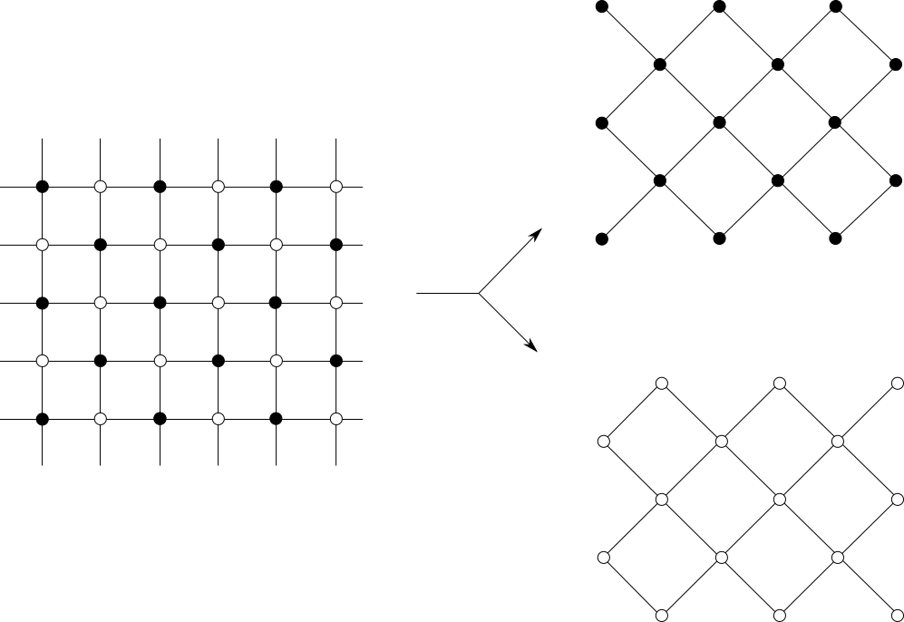
A splitting of $\mathbb{Z}^{2}$ into two graphs can be obtained by decomposing the vertices into black vertices $\mathcal{V}:=\{(x,y)\;|\;x+y=0\mod 2\}$ and white vertices $\mathcal{V}^{*}:=\{(x,y)\;|\;x+y=1\mod 2\}$ and by taking the diagonals of $\mathbb{Z}^{2}$ as the new edges, see Figure 3. Then, one obtains two discrete nets, which are topologically dual to each other. By restricting $f:=\mathfrak{f}|_{\mathcal{V}(\mathcal{G})}$ and $f^{*}:=\mathfrak{f}^{*}|_{\mathcal{V}(\mathcal{G}^{*})}$ , it is easy to verify that $f$ and $f^{*}$ satisfy the definition (1.2) with ${R}_{ij}=0$ and ${R}_{ij}^{*}=0$ for all edges $e_{ij}$ and $e_{ij}^{*}$ .

Refer to caption — Figure 3. Decomposition of $\mathbb{Z}^{2}$ into graphs with black and white vertices.

Remark 1.3.

The same procedure as above can be taken to generate isothermic parametrized constant mean curvature surfaces (both minimal and CMC) in our setting from the traditional ones over $\mathbb{Z}^{2}$ . However, general members in the associated family of an isothermic parametrized constant mean curvature surface do not have the factorized cross-ratio property, and thus they are not an isothermic parametrized surface. Moreover, $R_{ij}$ and $R_{ij}^{*}$ are not zero, thus they are not even an isothermic surface in the sense of Lam and Pinkall [12].

Example 2 (Face-edge-constraint minimal surfaces).

Lam [10] showed that two types of discrete minimal surfaces, namely the A-minimal surface from integrable system and the C-minimal surface obtained from variational principle, can be related with an associated family. In [6] showed that the family of minimal surfaces can be interpreted by the face-edge-constraint minimal surfaces. Specifically, a discrete surface $f:\mathcal{V}(\mathcal{G})\rightarrow\mathbb{R}^{3}$ with normal defined on faces $n:\mathcal{F}(\mathcal{G})\rightarrow S^{2}$ is called face-edge-constraint if

(1.7)

(n_{i}+n_{j})\perp df_{ij}

holds for every edges $e_{ij}\in\mathcal{E}(\mathcal{G})$ . For such nets one can define the integrated mean curvature for edges by

\mathbf{H}_{ij}=\frac{1}{2}\lvert df_{ij}\rvert\tan\frac{\theta_{ij}}{2},

where $\theta_{ij}$ is the bending angle between the planes $P_{i}:=\mathrm{span}\{n_{i},df_{ij}\}$ and $P_{j}:=\mathrm{span}\{n_{j},df_{ij}\}$ . The face-edge-constraint minimal surface in this setting is naturally defined by the surface with vanishing integrated mean curvature for every faces, i.e., $\mathbf{H}_{i}:=\sum_{j}\mathbf{H}_{ij}=0$ .

By a simple calculation (Proposition 3.8 in [6]) we have

(1.8)

E_{ij}^{-1}\cdot n_{i}\cdot E_{ij}=-n_{j}.

Let the real part $R_{ij}:=2\mathbf{H}_{ij}$ and $R^{*}_{ij}=0$ , i.e., $E_{ij}=2\mathbf{H}_{ij}+df_{ij}$ and $E_{ij}^{*}=df^{*}_{ij}$ . Moreover, define $f^{*}=n$ . It is easy to show that the face-edge-constraint minimal surface satisfies the isothermic condition with the normal being the dual surface:

\sum_{j}E_{ij}\cdot E^{*}_{ij}=\sum_{j}E_{ij}\cdot(n_{j}-n_{i})=\sum_{j}(-n_{i}\cdot E_{ij}-E_{ij}\cdot n_{i})=0\quad\mbox{for all $i$},

where for the second equality we use (1.8) and $\sum_{j}E_{ij}=0$ in the last equality which follows from the minimality condition $\mathbf{H}_{i}=\sum_{j}\mathbf{H}_{ij}=\sum_{j}R_{ij}/2=0$ .

Given any discrete net $f:\mathcal{V}(\mathcal{G})\rightarrow\mathbb{R}^{3}$ and its dual $f^{*}:\mathcal{V}(\mathcal{G}^{*})\rightarrow\mathbb{R}^{3}$ , one can associate each edge, denoted by $(f_{0},f_{2})$ , and its dual edge, denoted by $(f^{*}_{1},f^{*}_{3})$ , with an elementary quadrilateral with vertices $f_{0}$ , $f^{*}_{1}$ , $f_{2}$ and $f^{*}_{3}$ .

Together with the definition of isothermic surfaces in Definition 1, the following definition for isothermic constant mean curvature surfaces is the main results in this paper.

Definition 2 (Geometric definition of constant mean curvature surfaces on general graphs).

Let $f$ and $f^{*}$ be a discrete isothermic surface and its Christoffel dual surface in Definition 1. Moreover, for every elementary quadrilateral $(v_{0},v_{1},v_{2},v_{3})$ on $\mathcal{D}$ (constructed by $\mathcal{G}$ and $\mathcal{G}^{*}$ ) with $v_{0},v_{2}\in\mathcal{V}(\mathcal{G})$ and $v_{1},v_{3}\in\mathcal{V}(\mathcal{G}^{*})$ , denote $E_{02}(=R_{02}+df_{02})$ to be the hyperedge associated with the edge $e_{02}\in\mathcal{E}(\mathcal{G})$ .

(1)

( $f$ , $f^{*}$ ) is called a pair of non-zero constant mean curvature surfaces (CMC surfaces in short) if the following two equations hold $:$

(1.9)

\left\{\begin{array}[]{l}\displaystyle f^{*}_{3}-f_{2}=E^{-1}_{02}\cdot(f_{0}-f^{*}_{1})\cdot E_{02},\\[5.69046pt] \displaystyle f^{*}_{3}-f_{0}=E^{-1}_{02}\cdot(f_{2}-f^{*}_{1})\cdot E_{02}.\end{array}\right.

(2)

$f$ is called a minimal surface if $f^{*}$ takes values in the unit two sphere $S^{2}$ and the following two equations hold $:$

(1.10)

\left\{\begin{array}[]{l}f^{*}_{3}=-E^{-1}_{02}\cdot f^{*}_{1}\cdot E_{02},\\[5.69046pt] \sum_{j}R_{ij}=0\quad\mbox{hold for all $i\in\mathcal{V}(\mathcal{G})$,}\end{array}\right.

where the sum takes such that $j$ are vertices adjacent to the vertex $i$ .

Figure 4. An elementary parallelogram.

Remark 1.4.

(1)

If $(f,f^{*})$ is a pair of discrete isothermic CMC surfaces with hyperedges $E_{ij}=R_{ij}+df_{ij}$ and $E^{*}_{ij}=R^{*}_{ij}+df^{*}_{ij}$ , then, $(f^{*},f)$ is also a pair of discrete isothermic CMC surface with hyperedges $E^{*}_{ij}=R_{ij}+df^{*}_{ij}$ and $E_{ij}=R^{*}_{ij}+df_{ij}$ .
(2)

Definition 2 (1) implies that the quadrilateral has the opposite edges with equal length, i.e., $\lvert f^{*}_{1}-f_{0}\rvert=\lvert f_{2}-f_{3}^{*}\rvert$ and $\lvert f_{3}^{*}-f_{0}\rvert=\lvert f_{2}-f_{1}^{*}\rvert$ . Moreover, $f_{0}$ , $f^{*}_{1}$ , $f_{2}$ and $f^{*}_{3}$ form a equally-folded skew parallelogram, see Lemma 40 in [8], see Figure 4.
(3)

In Theorem 2.2 and Theorem 2.7, we will show that each member in the associated family of an isothermic constant mean curvature surface is an isothermic constant mean curvature surface in the sense of Definition 2.
(4)

In Theorem 2.7, we will show that a discrete CMC surface naturally converges to a discrete minimal surface in the sense of Definition 2 when the mean curvature parameter $H$ goes to $0$ .

1.2. Discrete holomorphic function: From cross-ratio systems to additive rational Toda systems

It is known [5] that smooth constant mean curvature surfaces can be constructed by holomorphic data (the Weierstrass type representation formula), which is the classical Weierstrass representation for minimal surfaces and the so-called DPW representation for CMC surfaces, respectively.

On quad graphs, a discrete analogue of this representation has been known in [1, 7]. We generalize this representation to discrete isothermic constant mean curvature surfaces on general graphs.

We first recall notion of discrete holomorphic functions on quad graphs.

Definition 3.

(1)

A function $\alpha:\mathcal{E}(\mathcal{D})\rightarrow\mathbb{C}$ is called a labelling if $\alpha(\mathfrak{e})=\alpha(\mathfrak{e}^{*})$ for any edge $\mathfrak{e}\in\mathcal{E}(\mathcal{D})$ and the values of two opposite edges on any quadrilateral are equal.
(2)

Let $\alpha:\mathcal{E}(\mathcal{D})\to\mathbb{C}$ be a labelling. Then a following system is called the cross-ratio system:

(1.11) $q(z_{0},z_{1},z_{2},z_{3}):=\frac{(z_{0}-z_{1})(z_{2}-z_{3})}{(z_{1}-z_{2})(z_{3}-z_{0})}=\frac{\alpha_{1}}{\alpha_{2}}$

holds for any elementary quadrilateral $(v_{0},v_{1},v_{2},v_{3})$ . Here we write $z_{i}=z(v_{i})\;(i=0,1,2,3)$ , $\alpha_{1}=\alpha(\mathfrak{e}_{01})=\alpha(\mathfrak{e}_{32})$ and $\alpha_{2}=\alpha(\mathfrak{e}_{03})=\alpha(\mathfrak{e}_{12})$ for $\mathfrak{e}_{ij}\in\mathcal{E}(\mathcal{D})$ .

It is known [7] that a solution $z:\mathcal{V}(\mathcal{D})\to\mathbb{C}$ of the cross-ratio system (1.11) with $\alpha_{1}/\alpha_{2}=-1$ is called the discrete holomorphic function. By abuse of notation we also call any solution of the cross-ratio system (1.11) the discrete holomorphic function.

In [1] (for the case of minimal surfaces) and [7] (for the case of CMC surfaces), it has been proved that every solution of a cross-ratio system on $\mathcal{D}=\mathbb{Z}^{2}$ gives an isothermic parametrized constant mean curvature surface. Conversely, the extended frame of an isothermic parametrized constant mean curvature surface on $\mathcal{D}$ gives a solution of a cross-ratio system.

Here the extended frame is a map from $\mathcal{V}(\mathcal{D})$ into the loop group $\Lambda{\rm SU}_{2,\sigma}$ such that it gives naturally a constant mean curvature surface through the Sym-Bobenko formula (for the case of CMC surfaces) or a direct summation formula (for the case of minimal surfaces), see Section 2.1.

Moreover there were assumed that $\mathcal{D}$ is the square lattice $\mathbb{Z}^{2}$ and the labelling $\alpha$ takes values in $\mathbb{R}^{\times}$ and satifies

\frac{\alpha_{1}}{\alpha_{2}}<0.

In Section 2, we will generalize them to arbitrary quad-graphs $\mathcal{D}$ and arbitrary labellings $\alpha$ which take values in $\mathbb{C}^{\times}$ , and introduce the mean curvature parameter $H$ .

Figure 5. Bipartite decomposition

It is known [4] that the cross-ratio system (1.11) can be transformed as the three-leg form:

(1.12)

\frac{\alpha_{1}}{z_{0}-z_{1}}-\frac{\alpha_{2}}{z_{0}-z_{3}}=\frac{\alpha_{1}-\alpha_{2}}{z_{0}-z_{2}}.

Then adding all three-leg forms as in (1.12) around the vertex $v_{0}$ , see Figure 5, we obtain the equation which depends only on the filed $z$ in the black vertices $v_{2k}$ :

(1.13)

\sum_{k=1}^{n}\frac{\alpha_{k}-\alpha_{k+1}}{z_{0}-z_{2k}}=0.

Thus on general graphs, notion of holomorphicity is defined as follows.

Definition 4 ([4]).

Let $\mathcal{G}$ be any oriented cell decomposition of a surface.

(1)

The corner $\mathcal{C}(\mathcal{G})$ is a set of pairs $(i,m)$ of vertices $i\in\mathcal{V}(\mathcal{G})$ and faces $m\in\mathcal{F}(\mathcal{G})$ such that $i$ is incident to $m$ .
(2)

The additive rational Toda system on $\mathcal{G}$ is a map $z:\mathcal{V}(\mathcal{G})\rightarrow\mathbb{C}$ together with a corner map $\alpha:\mathcal{C}(\mathcal{G})\rightarrow\mathbb{C}$ such that

(1.14) $\alpha_{i,m}=\alpha_{j,n}\quad\text{for all edges $e_{ij}\in\mathcal{E}(\mathcal{G})$,}$

and

(1.15) $\sum_{j}\frac{\alpha_{i,m}-\alpha_{j,m}}{z_{i}-z_{j}}=0\quad\text{for all vertices $i\in\mathcal{V}(\mathcal{G})$,}$

where the index $j$ runs over all the edges $(ij)$ incident to the vertex $i$ and $m$ is the left face to $e_{ij}$ .

It is easy to see that for a double graph $\mathcal{D}$ given by $\mathcal{V}(\mathcal{D})=\mathcal{V}(\mathcal{G})\cup\mathcal{V}(\mathcal{G}^{*})$ , a labelling $\alpha:\mathcal{E}(\mathcal{D})\to\mathbb{C}$ gives a corner $\mathcal{C}(\mathcal{G})\to\mathbb{C}$ which satisfies (1.14). Thus a cross-ratio system (1.11) on $\mathcal{D}$ gives an additive rational Toda system (1.15) on $\mathcal{G}$ . We remark that the cross-ratio system on $\mathcal{D}$ also gives an additive rational Toda system on $\mathcal{G}^{*}$ (the so-called dual additive rational Toda system), see Section 3.2.

Figure 6. Additive rational Toda system.

Remark 1.5.

The additive rational Toda system induces the discrete holomorphic quadratic differential [11] in the following way. Recall that the holomorphic quadratic differential is defined by a map $q:\mathcal{E}(\mathcal{G})\rightarrow\mathbb{C}$ such that

(1.16)		$\displaystyle\sum_{j}q_{ij}=0,\quad\text{for all vertex $i\in\mathcal{V}(\mathcal{G})$},$
(1.17)		$\displaystyle\sum_{j}\frac{q_{ij}}{z_{i}-z_{j}}=0,\quad\text{for all vertex $i\in\mathcal{V}(\mathcal{G})$},$

where $j$ runs through all the neighbouring vertices of $i$ . Suppose given an additive rational Toda system. Let $q_{ij}:=\alpha_{i,m}-\alpha_{j,m}$ where $m$ is the left face of the edge $e_{ij}$ . By (1.14) we have $q_{ij}=q_{ji}$ and $q$ well-defined at the un-oriented edge. Then (1.17) is clearly satisfied. A simple calculation shows that it satisfies (1.16). Besides, the induced holomorphic quadratic differential satisfies one more additional condition

\sum_{ij}q_{ij}=0,\quad\text{for all face $k\in\mathcal{F}(\mathcal{G})$},

where $(ij)$ runs through all the edges around the face $k$ .

The other main result in this paper is a representation formula for isothermic constant mean curvature surfaces for general graphs in terms of solutions (the so-called normalized potentials) of additive Rational Toda systems.

Theorem 1.6 (The Weierstrass type representation for isothermic constant mean curvature surfaces).

Every solution of an additive rational Toda system on a general graph $\mathcal{G}$ gives an isothermic constant mean curvature surface. Conversely, the extended frame of an isothermic constant mean curvature surface on $\mathcal{G}$ gives a solution of an additive rational Toda system.

The precise statements and proofs will be given in Theorem. 4.1 and Theorem. 4.4.

Remark 1.7.

Here the extended frame for general isothermic constant mean curvature surfaces has not been known, and thus we will give a definition for it in Section 4 by using the Weierstrass type representation. Note that the extended frames will naturally induce isothermic constant mean curvature surfaces by the Sym-Bobenko formula.

2. Discrete constant mean curvature surfaces on quadrilateral nets

It is known [2, 1] that discrete isothermic parametrized constant mean curvature surfaces are defined on $\mathbb{Z}^{2}$ and obtained from the extended frames. In this section we extend the basic construction of the extended frames for constant mean curvature surfaces on even quad-graphs $\mathcal{D}$ and generalize them using the mean curvature $H$ and the Hopf differential $\alpha$ , which takes values in $\mathbb{C}^{\times}$ .

2.1. The extended frames and construction of constant mean curvature surfaces

Recall that the extended frame of a discrete isothermic parametrized CMC surfaces on $\mathbb{Z}^{2}$ from [2, (4.14)]: The extended frame $\Phi_{n,m}$ is given by the transition matrices $U$ , $V$ defined by $\Phi_{n+1,m}=U\Phi_{n,m}$ and $\Phi_{n,m+1}=V\Phi_{n,m}$ , where

(2.1)

\left\{\begin{array}[]{l}\displaystyle U=\frac{1}{p}\begin{pmatrix}a&-\lambda u-\lambda^{-1}u^{-1}\\ \lambda u^{-1}+\lambda^{-1}u&\bar{a}\\ \end{pmatrix}\\[8.5359pt] \displaystyle V=\frac{1}{q}\begin{pmatrix}b&-i\lambda v+i\lambda^{-1}v^{-1}\\ i\lambda v^{-1}-i\lambda^{-1}v&\bar{b}\\ \end{pmatrix}\end{array}\right.,

with

p^{2}=\det U=\lambda^{2}+\lambda^{-2}+|a|^{2}+u^{2}+u^{-2},\quad q^{2}=\det V=-\lambda^{2}-\lambda^{-2}+|b|^{2}+v^{2}+v^{-2}.

Here $a,b$ take values in $\mathbb{C}$ and $u,v$ take values in $\mathbb{R}^{\times}$ . The important ansatz about $p$ and $q$ is as follows:

(2.2)

The zeros of

p

and

q

with respect to

\lambda

are

m

- and

n

-independent, respectively.

Denote square of the zeros of $p$ by $\alpha,\alpha^{-1}$ and square of the zeros of $q$ by $\beta,\beta^{-1}$ . It is easy to see that from the form of $p$ and $q$ , $\alpha$ is negative and $\beta$ is positive and thus the zeros of $p$ are always pure imaginary valued and the zeros of $q$ are always real valued. Moreover, it always holds

(2.3)

\frac{\alpha}{\beta}<0.

We then rephrase $p^{2}$ and $q^{2}$ by

p^{2}=-\alpha^{-1}(1-\lambda^{2}\alpha)(1-\lambda^{-2}\alpha),\quad q^{2}=\beta^{-1}(1-\lambda^{2}\beta)(1-\lambda^{-2}\beta).

The ansatz (2.2) for $\alpha$ and $\beta$ can be understood as a labelling, i.e., $\alpha$ satisfies the condition $(1)$ in Definition 3.

We now generalize the formulation of the extended frame (2.1) to arbitrary even quad graph $\mathcal{D}$ with the constant mean curvature parameter $H\in\mathbb{R}$ and the Hopf differential $\alpha:\mathcal{D}\to\mathbb{C}^{\times}$ which is a labelling. Note that $\alpha$ is not necessary real-valued and we do not assume the condition (2.3).

Definition 5.

The extended frame $\Phi=\Phi(v_{i},\lambda)$ is defined to be a map from $\mathcal{V}(\mathcal{D})$ into the loop group $\Lambda{\rm SU}_{2,\sigma}$ , i.e., a set of maps from the unit circle $S^{1}$ of the complex plane into the unitary group of degree two ${\rm SU}_{2}$ such that it satisfies the following relation for each edge $\mathfrak{e}=(v_{i},v_{j})\in\mathcal{E}(\mathcal{D})$ :

(2.4)		$\displaystyle\Phi(v_{j},\lambda)=\frac{1}{\kappa(\mathfrak{e},\lambda)}U(\mathfrak{e},\lambda)\Phi(v_{i},\lambda),$
where
(2.5)		$\displaystyle U(\mathfrak{e},\lambda)=\begin{pmatrix}d&\lambda^{-1}Hu-\lambda\bar{\alpha}\bar{u}^{-1}\\ \lambda^{-1}\alpha u^{-1}-\lambda H\bar{u}&\bar{d}\end{pmatrix},$
and
(2.6)		$\displaystyle\kappa(\mathfrak{e},\lambda)=\sqrt{\det U(\mathfrak{e},\lambda)}=\sqrt{(1-\lambda^{-2}H\alpha)(1-\lambda^{2}H\bar{\alpha})}.$

Here $u=u(\mathfrak{e})$ and $d=d(\mathfrak{e})$ are assumed to take values in $\mathbb{C}$ , and $\alpha=\alpha(\mathfrak{e})$ is assumed to be a labelling on $\mathcal{D}$ which takes values in $\mathbb{C}^{\times}$ and satisfies $|\sqrt{H\alpha}|\neq 1$ and $\arg\alpha_{1}\neq\arg\alpha_{2}$ , where $\alpha_{1}=\alpha_{01}=\alpha_{32}$ and $\alpha_{2}=\alpha_{03}=\alpha_{12}$ , on any elementary quadrilateral $(v_{0},v_{1},v_{2},v_{3})$ . The function $\alpha$ will be called the Hopf differential and the real constant parameter $H$ will be called the mean curvature.

The precise definition of the loop group $\Lambda{\rm SU}_{2,\sigma}$ can be found in Appendix A.

Remark 2.1.

(1)

The assumption $\sqrt{H\alpha}\neq 1$ is necessary, since $\Phi$ needs to be an element in $\Lambda{\rm SU}_{2,\sigma}$ . If we use the $r$ -loop group $\Lambda^{r}\mathrm{SU}_{2,\sigma}$ with suitable $1\geq r>0$ , then this assumption can be removed. The assumption $\arg\alpha_{1}\neq\arg\alpha_{2}$ is necessary to normalize the determinant of $U$ having the form in (2.6), see $(2)$ .

(2)

The form of $\kappa$ in (2.6) is not a restriction but it can be automatically satisfied. In fact when $H=0$ , then it is easily normalized as in (2.6) by scaling of $U$ with $1/\sqrt{\det U}=1/\sqrt{|d|^{2}+|\alpha|^{2}|u|^{-2}}$ , and when $H\neq 0$ , the determinant of $U$ can be computed as

	$\displaystyle\det U$	$\displaystyle=\|d\|^{2}+H^{2}\|u\|^{2}+\|\alpha\|^{2}\|u\|^{-2}-\lambda^{-2}H\alpha-\lambda^{-2}H\bar{\alpha}$
		$\displaystyle=H\|\alpha\|\left(p-\lambda^{-2}e^{\sqrt{-1}\arg\alpha}-\lambda^{-2}e^{-\sqrt{-1}\arg\alpha}\right),$

where $p=H^{-1}|\alpha|^{-1}|d|^{2}+H|\alpha|^{-1}|u|^{2}+H^{-1}|\alpha||u|^{-2}$ . Then it is easy to see that $p\geq 2$ or $p\leq-2$ , and the labelling property of $\alpha$ , $\arg\alpha_{1}\neq\arg\alpha_{2}$ and the compatibility condition of $U$ imply that the zeros of $\det U$ give also a labelling, i.e., $\det U$ is a labelling.

Then by scaling a suitable real scalar function $q(\mathfrak{e})$ which is a labelling on $U(\mathfrak{e},\lambda)$ , we can assume without loss of generality that the zeros of $\kappa$ are $\alpha$ , i.e., $\kappa$ has the form in (2.6). More precisely, take $q$ as a solution of $H^{2}|\alpha|^{2}q^{4}-(|d|^{2}+H^{2}|u|^{2}+|\alpha|^{2}|u|^{-2})q^{2}+1=0$ , and define $\tilde{\alpha}$ as $\tilde{\alpha}=q^{2}\alpha$ , then $\tilde{\alpha}$ is a zero of $q\kappa$ . Note that by the above discussion, it is easy to see that $q$ is a labelling and thus $\tilde{\alpha}$ is also a labelling. Note that the scaled matrix $\tilde{U}=qU$ has the same form as in (2.5).

From the discrete extended frame we will construct a discrete CMC surface by the Sym-Bobenko formula.

Theorem 2.2.

Let $H$ be some non-zero constant and $\Phi$ be a the extended frame in (2.4). Moreover let $\lambda=e^{\sqrt{-1}t},\sigma_{3}=\operatorname{diag}(1,-1)$ . Define two maps into $\operatorname{Im}\mathbb{H}\cong\mathbb{R}^{3}$ as follows $:$

(2.7)

\left\{\begin{array}[]{ll}\displaystyle\mathfrak{f}&=\displaystyle-\frac{1}{H}\left(\Phi^{-1}\partial_{t}\Phi-\frac{\sqrt{-1}}{2}\operatorname{Ad}\Phi^{-1}(\sigma_{3})\right)\Big|_{t\in\mathbb{R}},\\[8.5359pt] \displaystyle\mathfrak{f}^{*}&=\displaystyle-\frac{1}{H}\left(\Phi^{-1}\partial_{t}\Phi+\frac{\sqrt{-1}}{2}\operatorname{Ad}\Phi^{-1}(\sigma_{3})\right)\Big|_{t\in\mathbb{R}}.\end{array}\right.

Then the following statements hold $:$

(1)

If $\alpha$ is a real valued and $t=0$ , then $\mathfrak{f}$ and $\mathfrak{f}^{*}$ are respectively a discrete isothermic parametrized CMC surface and its Christoffel dual isothermic parametrized CMC surface.
(2)

For any non-zero complex valued labelling $\alpha$ and any $t\in\mathbb{R}$ and a decomposition $\mathcal{V}(\mathcal{D})=\mathcal{V}(\mathcal{G})\cup\mathcal{V}(\mathcal{G}^{*})$ , define two maps $f=\mathfrak{f}|_{\mathcal{V}(\mathcal{G})}$ and $f^{*}=\mathfrak{f}^{*}|_{\mathcal{V}(\mathcal{G}^{*})}$ . Then $f$ and $f^{*}$ are respectively a discrete CMC surface and its Christoffel dual CMC surface in the sense of Definition 2.

The statement (1) is the result in [2] with $\mathcal{D}=\mathbb{Z}^{2}$ and a slight modification on notation. We will prove it in Appendix C.

To prove (2), we need the following Lemmata.

Lemma 2.3.

Let $\mathfrak{f}$ be a map defined by the Sym-Bobenko formula (2.7). Define an edge $\mathfrak{E}_{ij}=\mathfrak{R}_{ij}+d\mathfrak{f}_{ij}:\mathcal{E}(\mathcal{D})\to\mathbb{H}$ by

(2.8)

\mathfrak{R}_{ij}:=\frac{1}{2H}\partial_{t}(\log\det U_{ij})|_{t\in\mathbb{R}}\in\mathbb{R}.

Then $\mathfrak{E}_{ij}$ is the normal transport vector, i.e.,

\mathfrak{E}_{ij}^{-1}\cdot\mathfrak{n}_{j}\cdot\mathfrak{E}_{ij}=-\mathfrak{n}_{i},

where $\mathfrak{n}$ is the unit normal to a surface $\mathfrak{f}$ given by $\mathfrak{n}=\frac{\sqrt{-1}}{2}\operatorname{Ad}\Phi^{-1}(\sigma_{3})|_{t\in\mathbb{R}}$ .

Proof.

The edge $\mathfrak{E}_{ij}$ can be rephrased as

(2.9)	$\displaystyle\mathfrak{E}_{ij}$	$\displaystyle=\frac{1}{2H}\partial_{t}(\log\det U_{ij})+\mathfrak{f}_{j}-\mathfrak{f}_{i}$
	$\displaystyle=-\frac{1}{H}\Phi_{j}^{-1}\left(-\left(\partial_{t}\kappa_{ij}^{-1}\right)U_{ij}+\partial_{t}\left(\kappa_{ij}^{-1}U_{ij}\right)-\frac{\sqrt{-1}}{2}[\sigma_{3},\kappa_{ij}^{-1}U_{ij}]\right)\Phi_{i}$
	$\displaystyle=-\frac{1}{\kappa_{ij}H}\Phi_{j}^{-1}\left(\partial_{t}U_{ij}-\frac{\sqrt{-1}}{2}[\sigma_{3},U_{ij}]\right)\Phi_{i}.$

Since $\partial_{t}U_{ij}-\frac{\sqrt{-1}}{2}[\sigma_{3},U_{ij}]$ is an off-diagonal matrix, the claim $\mathfrak{E}_{ij}^{-1}\cdot\mathfrak{n}_{j}\cdot\mathfrak{E}_{ij}=-\mathfrak{n}_{i}$ easily follows. ∎

Remark 2.4.

(1)

From (2.8), it is clear that $\mathfrak{R}_{ij}=\mathfrak{R}_{ji}$ and on any elementary quadrilateral $(v_{0},v_{1},v_{2},v_{3})$ , $\mathfrak{R}_{01}=\mathfrak{R}_{32}$ and $\mathfrak{R}_{03}=\mathfrak{R}_{12}$ from the labelling property.

(2)

A similar statement holds for the map $\mathfrak{f}^{*}$ , i.e., there exists an edge $\mathfrak{E}_{ij}^{*}=\mathfrak{R}^{*}_{ij}+d\mathfrak{f}_{ij}^{*}$ such that $(\mathfrak{E}_{ij}^{*})^{-1}\cdot\mathfrak{n}_{j}\cdot\mathfrak{E}_{ij}^{*}=-\mathfrak{n}_{i}$ holds. In fact, one can choose $\mathfrak{R}^{*}_{ij}=\mathfrak{R}_{ij}$ and

\mathfrak{E}_{ij}^{*}=-\frac{1}{\kappa_{ij}H}\Phi_{j}^{-1}\left(\partial_{t}U_{ij}+\frac{\sqrt{-1}}{2}[\sigma_{3},U_{ij}]\right)\Phi_{i}

holds.

Defining that $f=\mathfrak{f}|_{\mathcal{V}(\mathcal{G})}$ and $f^{*}=\mathfrak{f}^{*}|_{\mathcal{V}(\mathcal{G}^{*})}$ , we build the diagonal hyperedges as

\displaystyle{E}_{02}:=R_{02}+df_{02},\quad{E}^{*}_{31}:=R_{31}+df^{*}_{31},

where $R_{02}=-\mathfrak{R}_{30}+\mathfrak{R}_{32}$ and $R_{31}=\mathfrak{R}_{30}+\mathfrak{R}_{01}$ . We define the hyperedges across the primal and dual nets by:

(2.10)		$\displaystyle E_{32}:=R_{32}+f_{2}-f_{3}^{},\quad E_{30}:=R_{30}+f_{0}-f_{3}^{},$
(2.11)		$\displaystyle E_{01}:=R_{01}+f_{1}^{}-f_{0},\quad E_{21}:=R_{21}+f_{1}^{}-f_{2}.$

where $R_{ij}=\mathfrak{R}_{ij}$ for $(ij)\in\{(01),(12),(32),(03)\}$ . Then $E_{02}$ and $E_{31}^{*}$ can be written as

E_{02}=-E_{30}+E_{32}=-E_{21}+E_{01},\quad E_{31}^{*}=E_{30}+E_{01}=E_{32}+E_{21}.

Lemma 2.5.

Let $E_{01}$ , $E_{12}$ , $E_{23}$ and $E_{03}$ be the hyperedges defined in (2.10) and (2.11), respectively. Then the following statement holds $:$

(2.12)		$\displaystyle\|E_{32}\|=\|E_{01}\|=\frac{\sqrt{\kappa_{1}^{2}+\operatorname{Re}(\lambda^{2}H\alpha_{1})}}{\kappa_{1}H},$
(2.13)		$\displaystyle\quad\|E_{12}\|=\|E_{03}\|=\frac{\sqrt{\kappa_{2}^{2}+\operatorname{Re}(\lambda^{2}H\alpha_{2})}}{\kappa_{2}H},$
(2.14)		$\displaystyle E_{12}\cdot E_{01}=E_{32}\cdot E_{03},$

where $\kappa_{1}=\kappa_{01}=\kappa_{32}$ and $\kappa_{2}=\kappa_{03}=\kappa_{12}$ . Moreover, by using (2.12), (2.14) is equivalent with

(2.15)

E_{23}=E_{02}^{-1}\cdot E_{10}\cdot E_{02}.

Note that $E_{ji}=\overline{E_{ij}}$ with $(ij)\in\{(01),(12),(32),(03)\}$ . Similary

(2.16)

E_{32}\cdot E_{03}=E_{12}\cdot E_{01}

holds, and by using (2.13), (2.16) is equivalent with

(2.17)

E_{12}=E_{02}^{-1}\cdot E_{03}\cdot E_{02}.

Proof.

We calculate $E_{01},E_{03},E_{12}$ and $E_{32}$ by the Sym-Bobenko formula as

	$\displaystyle E_{01}$	$\displaystyle=R_{01}+f_{1}^{*}-f_{0}=-\frac{1}{\kappa_{1}H}\Phi_{1}^{-1}\cdot\mathfrak{U}_{01}\cdot\Phi_{0},\quad E_{03}$	$\displaystyle=R_{03}+f_{3}^{*}-f_{0}=-\frac{1}{\kappa_{2}H}\Phi_{3}^{-1}\cdot\mathfrak{U}_{03}\cdot\Phi_{0},$
	$\displaystyle E_{12}$	$\displaystyle=R_{12}+f_{2}-f_{1}^{*}=-\frac{1}{\kappa_{2}H}\Phi_{2}^{-1}\cdot\mathfrak{U}_{12}\cdot\Phi_{1},\quad E_{32}$	$\displaystyle=R_{32}+f_{2}-f_{3}^{*}=-\frac{1}{\kappa_{1}H}\Phi_{2}^{-1}\cdot\mathfrak{U}_{32}\cdot\Phi_{3},$

where

	$\displaystyle\mathfrak{U}_{01}$	$\displaystyle=\partial_{t}U_{01}+\frac{\sqrt{-1}}{2}\sigma_{3}U_{01}+\frac{\sqrt{-1}}{2}U_{01}\sigma_{3},\quad\mathfrak{U}_{03}=\partial_{t}U_{03}-\frac{\sqrt{-1}}{2}\sigma_{3}U_{03}-\frac{\sqrt{-1}}{2}U_{03}\sigma_{3},$
	$\displaystyle\mathfrak{U}_{12}$	$\displaystyle=\partial_{t}U_{12}-\frac{\sqrt{-1}}{2}\sigma_{3}U_{12}-\frac{\sqrt{-1}}{2}U_{12}\sigma_{3},\quad\mathfrak{U}_{32}=\partial_{t}U_{32}+\frac{\sqrt{-1}}{2}\sigma_{3}U_{32}+\frac{\sqrt{-1}}{2}U_{32}\sigma_{3}.$

Clearly, (2.14) is equivalent to

\mathfrak{U}_{12}\cdot\mathfrak{U}_{01}=\mathfrak{U}_{32}\cdot\mathfrak{U}_{03}.

which is, by a direct calculation, equivalent to the compatibility condition

U_{12}U_{01}=U_{32}U_{03}.

Thus (2.14) holds. We now take the conjugation to (2.14), i.e.,

\overline{E_{03}}\cdot\overline{E_{32}}=\overline{E_{01}}\cdot\overline{E_{12}}.

Moreover, using (2.12) and $E_{02}=E_{32}-\overline{E_{03}}=E_{01}-\overline{E_{12}}$ , we have

E_{02}\cdot\overline{E_{32}}=\overline{E_{01}}\cdot E_{02}\Longleftrightarrow E_{02}\cdot E_{23}=E_{10}\cdot E_{02}.

Similary (2.16) follows and it is equivalent with (2.17). ∎

Proof of Theorem 2.2 (2).

It is easy to see that (2.15) and (2.17) imply

f^{*}_{3}-f_{2}=E^{-1}_{02}\cdot(f_{0}-f^{*}_{1})\cdot E_{02}\quad\mbox{and}\quad f^{*}_{3}-f_{0}=E^{-1}_{02}\cdot(f_{2}-f^{*}_{1})\cdot E_{02},

respectively. Thus Definition 2 (1) holds. Let us verify the isothermic condition (1.2) in Definition 1:

	$\displaystyle E_{02}\cdot E^{*}_{31}$	$\displaystyle=E_{02}\cdot(E_{30}+E_{01})$
		$\displaystyle=E_{02}\cdot E_{30}+E_{32}\cdot E_{02}$
		$\displaystyle=(E_{32}-E_{30})\cdot E_{30}+E_{32}\cdot(E_{32}-E_{30})$
		$\displaystyle=-E_{30}\cdot E_{30}+E_{32}\cdot E_{32}.$

In the second equality, we use the expression in (2.15). By symmetry, two terms above will be canceled with the terms in neighboring parallelogram, see Figure 7.

Figure 7.

Thus (1.2) holds. This completes the proof. ∎

Remark 2.6.

(1)

In [2], a map

$\mathfrak{f}_{K}=-\frac{1}{H}\left(\Phi^{-1}\partial_{t}\Phi\right)\big|_{t\in\mathbb{R}}$

has been called the discrete constant positive Gaussian curvature surface, since it is a parallel surface of a CMC surfaces $\mathfrak{f}$ and $\mathfrak{f}^{*}$ with distance $1/(2H)$ .
(2)

When the Hopf differential $\alpha$ is real-valued and $t\in\mathbb{R}^{\times}$ , $\mathfrak{f}$ (and $\mathfrak{f}^{*}$ ) was not known to satisfy any condition of isothermic parametrized surface, even though they are in fact isothermic surfaces in smooth case.

We next consider discrete minimal surfaces. Recall that the discrete minimal surface can be generated by the discrete Weierstrass representation, [1]: Let $z_{i}=z(v_{i})$ be a solution of the cross-ratio system (1.11) and take a dual solution of a cross-ratio system, i.e., $z^{*}$ is defined by

z_{i}^{*}-z_{j}^{*}:=\frac{\alpha_{ij}}{z_{j}-z_{i}},

and $z_{i}^{*}$ satisfies the cross-ratio system

q(z_{0}^{*},z_{1}^{*},z_{2}^{*},z_{3}^{*})=\frac{(z_{0}^{*}-z_{1}^{*})(z_{2}^{*}-z_{3}^{*})}{(z_{1}^{*}-z_{2}^{*})(z_{3}^{*}-z_{0}^{*})}=\frac{\alpha_{2}}{\alpha_{1}}

on any elementary quadrilateral $(v_{0},v_{1},v_{2},v_{3})$ , where $\alpha_{1}=\alpha_{01}=\alpha_{32},\alpha_{2}=\alpha_{03}=\alpha_{12}$ . Then a minimal surface is given by

(2.18)

d\mathfrak{f}_{ij}=\left.\frac{1}{2}\mathrm{Re}\left\{\frac{\lambda^{-2}\alpha_{ij}}{z_{j}^{*}-z_{i}^{*}}\left(1-z_{j}^{*}z_{i}^{*},\sqrt{-1}(1+z_{j}^{*}z_{i}^{*}),z_{j}^{*}+z_{i}^{*}\right)\right\}\right|_{\lambda=1},

and the normal $\mathfrak{n}:\mathbb{Z}^{2}\rightarrow S^{2}\subset\mathbb{R}^{3}\cong\mathbb{C}\times\mathbb{R}$ at vertices is given by

(2.19)

\displaystyle(\mathfrak{n}^{x}_{i}+\sqrt{-1}\mathfrak{n}^{y}_{i},\mathfrak{n}^{z}_{i})

\displaystyle=\left(\frac{2z_{i}^{*}}{1+\lvert z_{i}^{*}\rvert^{2}},\frac{\lvert z_{i}^{*}\rvert^{2}-1}{\lvert z_{i}^{*}\rvert^{2}+1}\right).

Here note that the Hopf differential $\alpha$ assumed to be real-valued.

We now show that the Sym-Bobenko formula in (2.7) converges to the discrete Weierstrass representation when $H$ goes to $0$ , and moreover, it defines a discrete minimal surface on a general graph $\mathcal{G}$ .

Theorem 2.7.

Retain the assumptions in Theorem 2.2.

(1)

When $H$ converges to $0$ , the formula (2.7) induces the discrete Weierstrass representation (2.18) and the dual surface $\mathfrak{f}^{*}$ becomes $\mathfrak{n}$ defined in (2.19).
(2)

For any non-zero complex-valued labelling $\alpha$ and any $t\in\mathbb{R}$ and the decomposition $\mathcal{V}(\mathcal{D})=\mathcal{V}(\mathcal{G})\cup\mathcal{V}(\mathcal{G}^{*})$ , $f=\mathfrak{f}|_{\mathcal{V}(\mathcal{G})}$ given by (2.18) is a discrete minimal surface with the dual surface $f^{*}=\mathfrak{f}^{*}|_{\mathcal{V}(\mathcal{G}^{*})}$ in the sense of Definition 2 (2).

Proof.

(1) When $H$ converges to $0$ , the compatibility condition of the discrete extended frame $\Phi$ in (2.4) can be explicitly obtained by the dual solution of a cross-ratio system: Define the frame $\Phi$ to be

(2.20)

\Phi_{i}=\Phi(v_{i},\lambda)=\frac{1}{\sqrt{1+|z_{i}^{*}|^{2}}}\begin{pmatrix}1&\bar{z}_{i}^{*}\lambda\\ -z_{i}^{*}\lambda^{-1}&1\end{pmatrix}.

Then the transition matrix $U_{ij}=\Phi_{j}\Phi_{i}^{-1}$ can be computed as

	$\displaystyle U_{ij}$	$\displaystyle=\frac{1}{\sqrt{(1+\|z_{i}^{}\|^{2})(1+\|z_{j}^{}\|^{2})}}\begin{pmatrix}1+\bar{z}_{i}^{}z_{j}^{}&-(\bar{z}_{i}^{}-\bar{z}_{j}^{})\lambda\\ (z_{i}^{}-z_{j}^{})\lambda^{-1}&1+z_{i}^{}\bar{z}_{j}^{}\end{pmatrix}$
		$\displaystyle=\frac{1}{\sqrt{(1+\|z_{i}^{}\|^{2})(1+\|z_{j}^{}\|^{2})}}\begin{pmatrix}1+\bar{z}_{i}^{}z_{j}^{}&-\frac{\overline{\alpha_{ij}}}{\bar{z}_{j}-\bar{z}_{i}}\lambda\\ \frac{\alpha_{ij}}{z_{j}-z_{i}}\lambda^{-1}&1+z_{i}^{}\bar{z}_{j}^{}\end{pmatrix}.$

Setting

(2.21)

u_{ij}=\frac{\alpha_{ij}}{z_{i}^{*}-z_{j}^{*}}\sqrt{(1+\lvert z_{i}^{*}\rvert^{2})(1+\lvert z_{j}^{*}\rvert^{2})},

we conclude $\Phi$ in (2.20) is the extended frame $\Phi$ in (2.4) with $H=0$ .

We now compute the convergence of the edge $d\mathfrak{f}_{ij}$ : By (2.7) the edge satisfies

(2.22)	$\displaystyle d\mathfrak{f}_{ij}$	$\displaystyle=-\frac{1}{H}\left(\Phi^{-1}_{j}\partial_{t}\Phi_{j}-\frac{\sqrt{-1}}{2}\operatorname{Ad}\Phi^{-1}_{j}(\sigma_{3})\right)+\frac{1}{H}\left(\Phi^{-1}_{i}\partial_{t}\Phi_{i}-\frac{\sqrt{-1}}{2}\operatorname{Ad}\Phi_{i}^{-1}(\sigma_{3})\right),$
	$\displaystyle=-\frac{1}{\kappa_{ij}H}\Phi_{j}^{-1}\cdot\left(\partial_{t}U_{ij}-\frac{\sqrt{-1}}{2}\sigma_{3}\cdot U_{ij}+\frac{\sqrt{-1}}{2}U_{ij}\cdot\sigma_{3}\right)\cdot\Phi_{i}+\frac{1}{2H\kappa_{ij}}\partial_{t}(\log\det U_{ij})\operatorname{id}$
	$\displaystyle=2\frac{\sqrt{-1}}{\kappa_{ij}}\Phi_{j}^{-1}\cdot\begin{pmatrix}0&u_{ij}\lambda^{-1}\\ \overline{u_{ij}}\lambda&0\end{pmatrix}\cdot\Phi_{i}+\frac{\sqrt{-1}}{\kappa_{ij}}\left(\frac{\lambda^{-2}\alpha_{ij}}{1-\lambda^{-2}H\alpha_{ij}}-\frac{\lambda^{2}\overline{\alpha_{ij}}}{1-\lambda^{2}H\bar{\alpha}_{ij}}\right)\operatorname{id}.$

Now we can take the limit of $d\mathfrak{f}_{ij}$ gauged by a matrix $\left(\begin{smallmatrix}\sqrt{\lambda}^{-1}&0\\ 0&\sqrt{\lambda}\end{smallmatrix}\right)$ as $H$ goes $0$ , i.e.,

\lim_{H\to 0}\left\{\operatorname{Ad}\begin{pmatrix}\sqrt{\lambda}^{-1}&0\\ 0&\sqrt{\lambda}\end{pmatrix}(d\mathfrak{f}_{ij})\right\},

and plugging (2.20) and (2.21) into (2.22), we obtain (2.18) by a straightforward computation. Note that $\lim_{H\to 0}\kappa_{ij}=1$ .

Form (2.7), we can rephrase the dual net in terms of the primal net and the normal:

\mathfrak{f}^{*}=\mathfrak{f}-\frac{\sqrt{-1}}{H}\operatorname{Ad}\Phi^{-1}(\sigma_{3}).

The first term of the right-hand side can be ignored since it has finite norm by (2.22). By normalization the second term is exactly (2.19). Therefore, the dual net can be understood by scaling limit of the unit normal $\mathfrak{n}$ .

(2) From (1) we know that the arguments for the proof of Theorem 2.2 also applies for minimal surfaces. Hence, by using the proof of (1.9) and taking $H\rightarrow 0$ we have (1.10), since $f_{0}$ and $f_{2}$ vanish by the scaling limit. Furthermore, $R_{02}=\mathfrak{R}_{30}-\mathfrak{R}_{32}$ also holds for minimal surfaces. Hence, the sum $\sum R_{ij}$ vanishes, where $ij$ runs through the diagonal edges enclosing the vertex $v_{3}$ in Figure 7, because $\mathfrak{R}_{30}$ and $\mathfrak{R}_{32}$ are canceled with the terms in the neighbouring quadrilaterals in Figure 7. ∎

3. The Weierstrass representation and additive rational Toda systems

In this section, applying the Birkhoff decomposition to the extended frame, we first obtain a discrete normalized potential (a solution of the cross-ratio system), and conversely a normalized potential gives the extended frames on $\mathcal{D}$ .

Moreover, we decompose the cross-ratio system into the additive rational Toda system and its dual. These basic results on quadrilateral net will be used in the construction of constant mean curvature surfaces on general graphs in Section 4.

3.1. Holomorphic potential and the Weierstrass type representation

From now on, if $H\neq 0$ , then we always assume $H\alpha$ (one of the zeros of $\det U$ ) is sufficiently large such that $|\sqrt{H\alpha}|>1$ . This condition is imposed by a technical reason of definitions of the loop groups, see the definition of $\Lambda^{-}{\rm SL}_{2}\mathbb{C}_{\sigma}$ in Appendix A. In fact, using the $r$ -loop group $\Lambda_{r}{\rm SL}_{2}\mathbb{C}_{\sigma}$ (which is defined as a set of map from the $C^{r}$ circle with $r<1$ instead of $S^{1}$ ), we can avoid this assumption, but for simplicity of the presentation, the condition is assumed.

Figure 8. Cross-ratio system on a quadrilateral

Following [4] one can rephrase the cross-ratio system with the following matrix form.

Definition 6.

Let $\Phi_{-}:\mathcal{V}(\mathcal{D})\to\Lambda^{-}_{*}{\rm SL}_{2}\mathbb{C}_{\sigma}$ . We call respectively $\Phi_{-}$ and $L_{-}$ the wave function and the holomorphic potential if they satisfy the following equation:

(3.1)

\displaystyle\Phi_{-}(v_{j},\lambda)=L_{-}(\mathfrak{e},\lambda)\Phi_{-}(v_{i},\lambda),

where

(3.2)

\displaystyle L_{-}(\mathfrak{e},\lambda)

\displaystyle=\dfrac{1}{\sqrt{1-H\alpha(\mathfrak{e})\lambda^{-2}}}\begin{pmatrix}1&H(z_{i}-z_{j})\lambda^{-1}\\ \dfrac{\alpha(\mathfrak{e})}{z_{i}-z_{j}}\lambda^{-1}&1\end{pmatrix},

and $\alpha=\alpha(\mathfrak{e})$ is the Hopf differential.

It is straightforward to verify that the compatibility condition of $L_{-}$ in Definition 6 is the cross-ratio system for $z_{i}=z(v_{i})$ in Definition 3 and vice versa. Thus Definitions 3 and 6 are equivalent. From the following theorem, we clearly see the reason that $L_{-}$ has been called the holomorphic potential.

Theorem 3.1.

Let $\Phi$ be the extended frame as in (2.4). Perform the Birkhoff decomposition of Theorem A.1 to $\Phi$ as

(3.3)

\Phi=\Phi_{+}\Phi_{-},

i.e., $\Phi_{-}:\mathcal{V}(\mathcal{D})\to\Lambda^{-}_{*}{\rm SL}_{2}\mathbb{C}_{\sigma}$ and $\Phi_{+}:\mathcal{V}(\mathcal{D})\to\Lambda^{+}{\rm SL}_{2}\mathbb{C}_{\sigma}$ . Then $\Phi_{-}$ and $L_{-}$ are respectively the wave function and the normalized potential.

The proof will be given in Appendix D.

We now consider the converse construction, which is commonly called the DPW representaition, based on another loop group decomposition, the Iwasawa decomposition. More precisely, we will show a construction of the extended frame from a holomorphic potential.

Let us start from a discrete holomorphic function $z:\mathcal{V}(\mathcal{D})\to\mathbb{C},z_{i}=z(v_{i})$ , as a solution of the cross-ratio system (1.11) with a given labelling $\alpha=\alpha(\mathfrak{e})\in\mathbb{C}^{\times}$ , and define a holomorphic potential $L_{-}$ as in (3.2). Moreover, let $\Phi_{-}(v_{i},\lambda)$ be the wave function from $\mathcal{V}(\mathcal{D})$ into the loop group $\Lambda^{-}{\rm SL}_{2}\mathbb{C}_{\sigma}$ , such that for each edge $\mathfrak{e}=(v_{i},v_{j})$ , $\Phi_{-}$ satisfies

(3.4)

\displaystyle\Phi_{-}(v_{j},\lambda)=L_{-}(\mathfrak{e},\lambda)\Phi_{-}(v_{i},\lambda).

Then the following theorem holds.

Theorem 3.2 (The Weierstrass type representation).

Retain the notation above. Perform the Iwasawa decomposition of Theorem A.2 to $\Phi_{-}$ as

(3.5)

\Phi_{-}=\Phi_{+}\Phi,

i.e., $\Phi:\mathcal{V}(\mathcal{D})\to\Lambda{\rm SU}_{2,\sigma}$ and $\Phi_{+}:\mathcal{V}(\mathcal{D})\to\Lambda^{+}{\rm SL}_{2}\mathbb{C}_{\sigma}$ . Then $\Phi$ is the extended frame in (2.4). Furthermore, by using Theorem 2.2, a discrete isothermic CMC surface is obtained from the normalized potential.

The proof will be given in Appendix D.

3.2. Holomorphic potential for additive rational Toda system

The cross-ratio system induces a dual solution on $\mathcal{D}$ , which is called the dual discrete holomorphic potential as follows: Let $z_{i}=z(v_{i})$ be a solution of the cross-ratio system (1.11). Define a function $z_{i}^{*}=z^{*}(v_{i})$ as

(3.6)

H(z_{i}^{*}-z_{j}^{*})=\frac{\alpha(\mathfrak{e})}{z_{j}-z_{i}}.

Then $z^{*}:\mathcal{V}(\mathcal{D})\to\mathbb{C}$ satisfies the cross-ratio system:

(3.7)

q(z_{0}^{*},z_{1}^{*},z_{2}^{*},z_{3}^{*})=\frac{(z_{0}^{*}-z_{1}^{*})(z_{2}^{*}-z_{3}^{*})}{(z_{1}^{*}-z_{2}^{*})(z_{3}^{*}-z_{0}^{*})}=\frac{\alpha_{2}}{\alpha_{1}}.

Thus $z^{*}$ is also a discrete holomorphic function and called a dual discrete holomorphic function. Moreover, the discrete normalized potential $L_{-}$ defined in (3.2) can be rephrased as

(3.8)

\displaystyle L_{-}^{*}(\mathfrak{e}^{*},\lambda)

\displaystyle=\dfrac{1}{\sqrt{1-H\alpha(\mathfrak{e}^{*})\lambda^{-2}}}\begin{pmatrix}1&\dfrac{\alpha(\mathfrak{e}^{*})}{z_{j}^{*}-z_{i}^{*}}\lambda^{-1}\\ H(z_{j}^{*}-z_{i}^{*})\lambda^{-1}&1\end{pmatrix}.

Note that $\alpha(\mathfrak{e}^{*})=\alpha(\mathfrak{e})$ . The matrix $L_{-}^{*}(\mathfrak{e},\lambda)$ is called the dual holomorphic potential. Accordingly, the dual wave function $\Phi_{-}^{*}$ can be defined as

(3.9)

\Phi_{-}^{*}(v_{i},\lambda)=L_{-}^{*}(\mathfrak{e}^{*},\lambda)\Phi_{-}^{*}(v_{j},\lambda).

Remark 3.3.

It is easy to see that $z^{*}$ actually gives a solution to the same system, see [4, Proposition 12]. The choices of $z_{i}$ and $z_{i}^{*}$ are unique up to the initial conditions.

As we discussed in Section 1.2, the cross-ratio system induces the addtive rational Toda system on $\mathcal{G}$ . Note that the dual cross-ratio system (3.6) also induces the dual additive rational Toda system on $\mathcal{G}^{*}$ . Thus the cross-ratio system induces the pair of additive rational Toda systems on $\mathcal{G}$ an $\mathcal{G}^{*}$ , respectively:

(3.10)

\sum_{k=1}^{n}\frac{\alpha_{k}-\alpha_{k+1}}{z_{0}-z_{2k}}=0\quad\mbox{and}\quad\sum_{k=1}^{n^{\prime}}\frac{\alpha_{k}-\alpha_{k+1}}{z^{*}_{1}-z^{*}_{2k+1}}=0.

Similar to the cross-ratio system, the additive rational Toda system can also be formulated by the matrix form. However, one needs to introduce a gauge transformations for $\Phi_{-}$ and $\Phi_{-}^{*}$ . This means that the wave function $\Phi_{-}$ as in (3.1) and its dual wave function $\Phi_{-}^{*}$ as in (3.9) should be gauged as

(3.11)

\left\{\begin{array}[]{l}\Phi_{-}(v_{i},\lambda)\longrightarrow\mathcal{P}_{-}(v_{i},\lambda)=A(v_{i},\lambda)\Phi_{-}(v_{i},\lambda)\quad\mbox{for}\quad v_{i}\in\mathcal{V}(\mathcal{G}),\\[2.84544pt] \Phi^{*}_{-}(v_{i},\lambda)\longrightarrow\mathcal{P}^{*}_{-}(v_{i},\lambda)=A^{*}(v_{i},\lambda)\Phi^{*}_{-}(v_{i},\lambda)\quad\mbox{for}\quad v_{i}\in\mathcal{V}(\mathcal{G}^{*}),\end{array}\right.

where

(3.12)

A(v_{i},\lambda)=\begin{pmatrix}1&Hz_{i}\lambda^{-1}\\ 0&1\end{pmatrix},\quad A^{*}(v_{i},\lambda)=\begin{pmatrix}1&0\\ -Hz^{*}_{i}\lambda^{-1}&1\end{pmatrix}.

Then the transition matrices, i.e., the holomorphic potentials $L_{-}(\mathfrak{e},\lambda)$ and $L_{-}^{*}(\mathfrak{e},\lambda)$ in (3.2) and (3.8), respectively, should be gauged accordingly:

(3.13)

\left\{\begin{array}[]{l}L_{-}(\mathfrak{e},\lambda)\longrightarrow\mathcal{L}_{-}(\mathfrak{e},\lambda)=A^{*}(v_{j},\lambda)L_{-}(\mathfrak{e},\lambda)(A(v_{i},\lambda))^{-1},\\[2.84544pt] L_{-}^{*}(\mathfrak{e},\lambda)\longrightarrow\mathcal{L}_{-}^{*}(\mathfrak{e},\lambda)=A(v_{j},\lambda)L_{-}^{*}(\mathfrak{e},\lambda)(A^{*}(v_{i},\lambda))^{-1}.\end{array}\right.

Here $\mathfrak{e}=(v_{i},v_{j})\in\mathcal{E}(\mathcal{D})$ . The motivation of this gauge transformation becomes clear through the following proposition which has been given in [4] except the third statement:

Proposition 3.4.

Figure 9. Transition matrices for additive rational Toda system.

In any quadrilateral $(v_{0},v_{1},v_{2},v_{3})$ on $\mathcal{D}$ , the following statements holds $:$

(1)

Let $\mathcal{L}_{-}^{*}(e_{\mathcal{G}^{*}},\lambda)$ be the diagonal transition matrix from $\mathcal{P}_{-}^{*}(v_{1},\lambda)$ to $\mathcal{P}_{-}^{*}(v_{3},\lambda)$ , i.e.,

$\mathcal{P}_{-}^{*}(v_{3},\lambda)=\mathcal{L}_{-}^{*}(e_{\mathcal{G}^{*}},\lambda)\mathcal{P}_{-}^{*}(v_{1},\lambda).$

Then $\mathcal{L}_{-}^{*}(e_{\mathcal{G}^{*}},\lambda)$ only depends on $z_{0}=z(v_{0})$ , $z_{2}=z(v_{2})$ and $\lambda$ . Therefore the gauged wave function $\mathcal{P}_{-}^{*}$ defined on $\mathcal{V}(\mathcal{G}^{*})$ only depends on a solution of the additive rational Toda system on $\mathcal{G}$ and $\lambda$ .
(2)

Let $\mathcal{L}_{-}(e_{\mathcal{G}},\lambda)$ be the dual diagonal transition matrix from $\mathcal{P}_{-}(v_{0},\lambda)$ to $\mathcal{P}_{-}(v_{2},\lambda)$ , i.e,

$\mathcal{P}_{-}(v_{2},\lambda)=\mathcal{L}_{-}(e_{\mathcal{G}},\lambda)\mathcal{P}_{-}(v_{0},\lambda).$

Then $\mathcal{L}_{-}(e_{\mathcal{G}},\lambda)$ only depends on $z_{1}^{*}=z^{*}(v_{1})$ , $z_{3}^{*}=z^{*}(v_{3})$ and $\lambda$ . Therefore the gauged wave function $\mathcal{P}_{-}$ defined on $\mathcal{V}(\mathcal{G})$ only depends a solution of the dual additive rational Toda system on $\mathcal{G}^{*}$ and $\lambda$ .
(3)

Let $\mathcal{L}_{-}(\mathfrak{e},\lambda)$ be the transition matrix from $\mathcal{P}_{-}^{*}(v_{1},\lambda)$ to $\mathcal{P}_{-}(v_{0},\lambda)$ , i.e.,

$\mathcal{P}_{-}(v_{0},\lambda)=\mathcal{L}_{-}(\mathfrak{e},\lambda)\mathcal{P}_{-}^{*}(v_{1},\lambda).$

Then $\mathcal{L}_{-}(\mathfrak{e},\lambda)$ only depends on $z_{0}=z(v_{0})$ , $z_{1}^{*}=z^{*}(v_{1})$ and $\lambda$ .

Proof.

The statements (1) and (2) have been proven in [4], but we give a brief proof for the sake of completeness.

(1): Recall that the three-leg form in (1.12)

\frac{\alpha_{1}}{z_{0}-z_{1}}-\frac{\alpha_{2}}{z_{0}-z_{3}}=\frac{\alpha_{1}-\alpha_{2}}{z_{0}-z_{2}},

and its equivalent form

(3.14)

\frac{\alpha_{1}}{z_{0}-z_{1}}z_{1}-\frac{\alpha_{2}}{z_{0}-z_{3}}z_{3}=\frac{\alpha_{1}-\alpha_{2}}{z_{0}-z_{2}}z_{2}.

From (3.14), it is easy to see that

(3.15)

\frac{\alpha_{1}}{z_{0}-z_{1}}z_{0}-\frac{\alpha_{2}}{z_{0}-z_{3}}z_{3}=\frac{\alpha_{1}z_{0}-\alpha_{2}z_{2}}{z_{0}-z_{2}}\quad\mbox{and}\quad\frac{\alpha_{1}}{z_{0}-z_{1}}z_{1}-\frac{\alpha_{2}}{z_{0}-z_{3}}z_{0}=\frac{\alpha_{1}z_{2}-\alpha_{2}z_{0}}{z_{0}-z_{2}}

hold. Then by using (1.12), (3.14) and (3.15), we compute

(3.16)		$\displaystyle\mathcal{L}_{-}^{}(e_{\mathcal{G}^{}},\lambda)$	$\displaystyle=\widetilde{L}_{-}(v_{3},v_{0},\lambda)\widetilde{L}_{-}(v_{0},v_{1},\lambda)$
		$\displaystyle=\frac{1}{\mathfrak{l}}\left\{\operatorname{id}+\frac{\lambda^{-2}}{z_{0}-z_{2}}\begin{pmatrix}H(\alpha_{2}z_{2}-\alpha_{1}z_{0})&H^{2}(\alpha_{1}-\alpha_{2})z_{0}z_{2}\lambda^{-1}\\ (\alpha_{2}-\alpha_{1})\lambda&H(\alpha_{1}z_{2}-\alpha_{2}z_{0})\end{pmatrix}\right\},$

where $\mathfrak{l}=\sqrt{(1-H\alpha_{1}\lambda^{-2})(1-H\alpha_{2}\lambda^{-2})}$ . The claim follows.

(2): Similarly, we compute

(3.17)		$\displaystyle\mathcal{L}_{-}(e_{\mathcal{G}},\lambda)$	$\displaystyle=\widetilde{L}_{-}(v_{0},v_{1},\lambda)\widetilde{L}_{-}(v_{1},v_{2},\lambda)$
		$\displaystyle=\frac{1}{\mathfrak{l}}\left\{\operatorname{id}+\frac{\lambda^{-2}}{z_{3}^{}-z_{1}^{}}\begin{pmatrix}H(\alpha_{2}z_{1}^{}-\alpha_{1}z_{3}^{})&(\alpha_{2}-\alpha_{1})\lambda\\ H^{2}(\alpha_{1}-\alpha_{2})z_{1}^{}z_{3}^{}\lambda^{-1}&H(\alpha_{1}z_{1}^{}-\alpha_{2}z_{3}^{})\end{pmatrix}\right\},$

where $\mathfrak{l}=\sqrt{(1-H\alpha_{1}\lambda^{-2})(1-H\alpha_{2}\lambda^{-2})}$ .

(3): For an edge $\mathfrak{e}=(v_{1},v_{0})\in\mathcal{E}(\mathcal{D})$ with $v_{0}\in\mathcal{G}$ and $v_{1}\in\mathcal{G}^{*}$ , we compute $\mathcal{L}_{-}(\mathfrak{e},\lambda)$ as

(3.18)		$\displaystyle\mathcal{L}_{-}(\mathfrak{e},\lambda)=\frac{1}{\sqrt{1-H\alpha_{1}\lambda^{-2}}}A^{*}(v_{0},\lambda)L_{-}(v_{0},v_{1},\lambda)(A(v_{1},\lambda))^{-1}$
	$\displaystyle=\frac{1}{\sqrt{1-H\alpha_{1}\lambda^{-2}}}\begin{pmatrix}1&0\\ -Hz_{0}^{}\lambda^{-1}&1\end{pmatrix}\begin{pmatrix}1&H(z_{1}-z_{0})\lambda^{-1}\\ (z_{0}^{}-z_{1}^{*})\lambda^{-1}&1\end{pmatrix}\begin{pmatrix}1&-Hz_{1}\lambda^{-1}\\ 0&1\end{pmatrix}$
	$\displaystyle=\frac{1}{\sqrt{1-H\alpha_{1}\lambda^{-2}}}\begin{pmatrix}1&-Hz_{0}\lambda^{-1}\\ -z_{1}^{}\lambda^{-1}&H(z_{0}z_{1}^{}-\alpha_{1})\lambda^{-2}+1\end{pmatrix}.$

Here we use the relation $z_{1}-z_{0}=\frac{\alpha_{1}}{z_{0}^{*}-z_{1}^{*}}$ , which is equivalent with

-z_{1}z_{1}^{*}-z_{0}z_{0}^{*}+z_{0}z_{1}^{*}+z_{1}z_{0}^{*}=\alpha_{1}.

Thus $\mathcal{L}_{-}(\mathfrak{e},\lambda)$ depends only $z_{0}$ , $z_{1}^{*}$ and $\lambda$ , not $z_{0}^{*}$ and $z_{1}$ . ∎

The above proposition implies that we only need a holomorphic data on $\mathcal{G}$ , $z:\mathcal{V}(\mathcal{G})\rightarrow\mathbb{C}$ and they induce a dual holomorphic data on $\mathcal{G}^{*}$ , i.e., $z^{*}:\mathcal{V}(\mathcal{G}^{*})\rightarrow\mathbb{C}$ . The function $z^{*}$ is determined up to a global translation $z^{*}(v_{i})\mapsto z^{*}(v_{i})+c$ for some constant $c\in\mathbb{C}$ . We will see that this global translation will not affect the CMC surfaces.

From the above observation, we arrive the following definition.

Definition 7.

Let $\mathcal{G}$ (resp. $\mathcal{G}^{*}$ ) be a graph with corner $\alpha$ which satisfies (1.14), and $z_{2k}$ (resp. $z_{2k-1}^{*}$ ) be a solution of the (resp. the dual) additive rational Toda system in (3.10).

(1)

The matrix-valued function $\mathcal{L}_{-}$ in (3.17) (resp. $\mathcal{L}_{-}^{*}$ in (3.16)) will be called the normalized potential on $\mathcal{G}$ (resp. $\mathcal{G}^{*}$ ), and the solution $\mathcal{P}_{-}$ (resp. $\mathcal{P}_{-}^{*}$ ) is called the wave function (resp. dual wave function) on $\mathcal{G}$ (resp. $\mathcal{G}^{*}$ ).
(2)

If the wave functions $\mathcal{P}_{-}$ and $\mathcal{P}_{-}^{*}$ in (1) are compatible, i.e., they are connected by $\mathcal{L}_{-}(\mathfrak{e},\lambda)$ as in (3.18), then the pair $(\mathcal{P}_{-},\mathcal{P}_{-}^{*})$ will be called the pair of wave functions on $(\mathcal{G},\mathcal{G}^{*})$ . Moreover, the pair $(\mathcal{L}_{-},\mathcal{L}_{-}^{*})$ will be called the pair of normalized potentials on $(\mathcal{G},\mathcal{G}^{*})$ .

4. Algebraic definition of Isothermic constant mean curvature surfaces for general graphs

In this section we give the algebraic definition of isothermic constant mean curvature surfaces for general graphs utilizing the Weierstrass type representation. In particular we first define the pair of extended frames of isothermic constant mean curvature surfaces for general graphs through the Iwasawa decomposition. We will then show that the pair of extended frames define the pair of normalized potentials through the Birkhoff decomposition.

4.1. The Weierstrass type representaition for general graphs

We start from a solution $z:\mathcal{V}(\mathcal{G})\to\mathbb{C},z_{i}=z(v_{i})$ , of the addtive rational Toda system (1.13) on $\mathcal{G}$ with a given corner function $\alpha=\alpha(\mathfrak{e})$ which satisfies (1.14). Moreover, let $\mathcal{L}_{-}$ be the normalized potential and $\mathcal{P}_{-}$ the the corresponding wave functions defined in Definition 7 (1).

Lemma 4.1.

Retain notation the above. Perform the Iwasawa decomposition of Theorem A.2 to $\mathcal{P}_{-}$ as $\mathcal{P}_{-}=\mathcal{P}_{+}\mathcal{P}$ i.e., $\mathcal{P}\in\Lambda{\rm SU}_{2,\sigma}$ and $\mathcal{P}_{+}\in\Lambda^{+}{\rm SL}_{2}\mathbb{C}_{\sigma}$ . Then $\mathcal{P}$ satisfies

(4.1)		$\displaystyle\mathcal{P}(v_{2},\lambda)=\frac{1}{\tau(e_{\mathcal{G}},\lambda)}\mathcal{U}(e_{\mathcal{G}},\lambda)\mathcal{P}(v_{0},\lambda),$
where
(4.2)		$\displaystyle\mathcal{U}(e_{\mathcal{G}},\lambda)=\begin{pmatrix}Ha\lambda^{-2}+b+Hc\lambda^{2}&-\bar{r}\lambda^{-1}-H\bar{q}\lambda-H^{2}\bar{p}\lambda^{3}\\ H^{2}p\lambda^{-3}+Hq\lambda^{-1}+r\lambda&H\bar{c}\lambda^{-2}+\bar{b}+H\bar{a}\lambda^{2}\end{pmatrix}$

and $\tau(e_{\mathcal{G}},\lambda)=\sqrt{\mathcal{U}(e_{\mathcal{G}},\lambda)}=\sqrt{(1-H\alpha_{1}\lambda^{-2})(1-H\bar{\alpha}_{1}\lambda^{2})(1-H\alpha_{2}\lambda^{-2})(1-H\bar{\alpha}_{2}\lambda^{2})}$ . Here $a=a(e_{\mathcal{G}}),b=b(e_{\mathcal{G}}),c=c(e_{\mathcal{G}}),p=p(e_{\mathcal{G}}),q=q(e_{\mathcal{G}})$ and $r=r(e_{\mathcal{G}})$ depend only on fields of $\mathcal{G}^{*}$ , i.e., a solution of the dual additive rational Toda system on $\mathcal{G}^{*}$ .

Proof.

From Proposition 3.4, it is clear that $\mathcal{P}_{-}(v_{2k},\lambda)$ only depend on the addtive rational Toda system on $\mathcal{G}^{*}$ . Therefore after Iwasawa decomposition for $\mathcal{P}_{-}(v_{2k},\lambda)$ the function $\mathcal{P}(v_{2k},\lambda)$ only depends on a function on $\mathcal{G}^{*}$ . We now compute the Maurer-Cartan form $\mathcal{P}(v_{2k},\lambda)$ . On a quadrilateral $(v_{0},v_{1},v_{2},v_{3})$ , a straightforward computation shows that

	$\displaystyle\mathcal{U}(e_{\mathcal{G}},\lambda)$	$\displaystyle=\tau(e_{\mathcal{G}},\lambda)\mathcal{P}(v_{2},\lambda)(\mathcal{P}(v_{0},\lambda))^{-1}$
		$\displaystyle=\tau(e_{\mathcal{G}},\lambda)(\mathcal{P}(v_{2},\lambda))^{-1}\mathcal{L}_{-}(e_{\mathcal{G}},\lambda)\mathcal{P}_{+}(v_{0},\lambda),$

where $\mathcal{L}_{-}(e_{\mathcal{G}})$ is given in (3.17). The right-hand side of the above equation has the form

\lambda^{-3}\begin{pmatrix}0&0\\ *&0\end{pmatrix}+\lambda^{-2}\begin{pmatrix}*&0\\ 0&*\end{pmatrix}+\cdots.

Since the left-hand side of the above equation multiplying $\tau^{-1}$ takes values in $\Lambda{\rm SU}_{2,\sigma}$ and $\tau$ takes values in $\mathbb{R}_{>0}$ , we have the form as in the first equation of (4.2). ∎

Remark 4.2.

A similar statement holds for $\mathcal{P}_{-}^{*}$ , i.e., for the Iwasawa decomposition to

\mathcal{P}_{-}^{*}=\mathcal{P}_{+}^{*}\mathcal{P}^{*},\quad\mathcal{P}^{*}\in\Lambda{\rm SU}_{2,\sigma}\quad\mbox{and}\quad\mathcal{P}_{+}^{*}\in\Lambda^{+}{\rm SL}_{2}\mathbb{C}_{\sigma},

and $\mathcal{P}^{*}$ satisfies

(4.3)		$\displaystyle\mathcal{P}^{}(v_{3},\lambda)=\frac{1}{\tau(e_{\mathcal{G}^{}},\lambda)}\mathcal{U}^{}(e_{\mathcal{G}^{}},\lambda)\mathcal{P}^{*}(v_{1},\lambda),$
where
	$\displaystyle\mathcal{U}^{}(e_{\mathcal{G}^{}},\lambda)=\begin{pmatrix}Ha^{}\lambda^{-2}+b^{}+Hc^{}\lambda^{2}&-H^{2}\overline{r^{}}\lambda^{-3}-H\overline{q^{}}\lambda^{-1}-\overline{p^{}}\lambda\\ p^{}\lambda^{-1}+Hq^{}\lambda+H^{2}\overline{r^{}}\lambda^{3}&H\overline{c^{}}\lambda^{-2}+\overline{b^{}}+H\overline{a^{}}\lambda^{2}\end{pmatrix}$

and $\tau(e_{\mathcal{G}^{*}},\lambda)=\sqrt{\det\mathcal{U}^{*}(\mathfrak{e}_{\mathcal{G}^{*}},\lambda)}=\sqrt{(1-H\alpha_{1}\lambda^{-2})(1-H\bar{\alpha}_{1}\lambda^{2})(1-H\alpha_{2}\lambda^{-2})(1-H\bar{\alpha}_{2}\lambda^{2})}$ . Here $a^{*}=a^{*}(e_{\mathcal{G}^{*}}),b^{*}=b^{*}(e_{\mathcal{G}^{*}}),c^{*}=c^{*}(e_{\mathcal{G}^{*}}),p^{*}=p^{*}(e_{\mathcal{G}^{*}}),q^{*}=q^{*}(e_{\mathcal{G}^{*}})$ and $r^{*}=r^{*}(e_{\mathcal{G}^{*}})$ depend only on fields of $\mathcal{G}$ , i.e., a solution of the dual additive rational Toda equation on $\mathcal{G}$ .

Proposition 4.3.

Assume that normalized potentials $\mathcal{L}_{-}$ and $\mathcal{L}_{-}^{*}$ are a pair of normalized potentials in the sense of Definition 7 (2). Then the pair of maps $(\mathcal{P},\mathcal{P}^{*})$ given by the Iwasawa decomposition to the pair of wave functions, i.e, $(\mathcal{P}_{-},\mathcal{P}_{-}^{*})=(\mathcal{P}_{+},\mathcal{P}_{+}^{*})(\mathcal{P},\mathcal{P}^{*})$ , satisfies the following system on any quadrilateral $(v_{0},v_{1},v_{2},v_{3})$ on $\mathcal{D}=\mathcal{G}\cup\mathcal{G}^{*}:$

(4.4)

\displaystyle\mathcal{P}^{*}(v_{1}^{*},\lambda)=\frac{1}{\kappa(\mathfrak{e},\lambda)}\mathcal{U}(\mathfrak{e},\lambda)\mathcal{P}(v_{0},\lambda),\quad\mathcal{P}(v_{2},\lambda)=\frac{1}{\kappa(\mathfrak{e},\lambda)}\mathcal{U}(\mathfrak{e},\lambda)\mathcal{P}^{*}(v_{1},\lambda),

where $\mathfrak{e}=(v_{0},v_{1})$ in the first equation and $\mathfrak{e}=(v_{1},v_{2})$ in the second equation and

\displaystyle\mathcal{U}(\mathfrak{e},\lambda)=\begin{pmatrix}a_{\mathfrak{e}}+b_{\mathfrak{e}}\lambda^{-2}&c_{\mathfrak{e}}\lambda+d_{\mathfrak{e}}\lambda^{-1}\\ -\overline{c_{\mathfrak{e}}}\lambda^{-1}-\overline{d_{\mathfrak{e}}}\lambda&\overline{a_{\mathfrak{e}}}+\overline{b_{\mathfrak{e}}}\lambda^{2}\end{pmatrix},\quad\mathcal{U}(\mathfrak{e},\lambda)=\begin{pmatrix}a_{\mathfrak{e}}^{*}+b_{\mathfrak{e}}^{*}\lambda^{2}&c_{\mathfrak{e}}^{*}\lambda+d_{\mathfrak{e}}^{*}\lambda^{-1}\\ -\overline{c_{\mathfrak{e}}^{*}}\lambda^{-1}-\overline{d_{\mathfrak{e}}^{*}}\lambda&\overline{a_{\mathfrak{e}}^{*}}+\overline{b_{\mathfrak{e}}^{*}}\lambda^{-2}\end{pmatrix},

and

\displaystyle\kappa(\mathfrak{e},\lambda)=\sqrt{\det(\mathcal{U}(\mathfrak{e},\lambda))}=\left\{\begin{array}[]{l}\sqrt{(1-H\alpha_{1}\lambda^{-2})(1-H\bar{\alpha}_{1}\lambda^{2})},\quad(\mathfrak{e}=(v_{0},v_{1}))\\[5.69046pt] \sqrt{(1-H\alpha_{2}\lambda^{-2})(1-H\bar{\alpha}_{2}\lambda^{2})},\quad(\mathfrak{e}=(v_{1},v_{2}))\end{array}\right..

Proof.

It is a straightforward computation similar to the proof of Lemma 4.1. ∎

Applying the Sym-Bobenko formula $\mathfrak{f}$ in (2.7) to $\mathcal{P}$ and the dual $\mathfrak{f}^{*}$ to $\mathcal{P}^{*}$ , we naturally have maps $f$ and $f^{*}$ on $\mathcal{G}$ and $\mathcal{G}^{*}$ , i.e., we define $f=\mathfrak{f}$ and $f^{*}=\mathfrak{f}^{*}$ , and call $f$ and $f^{*}$ the primal surface and the dual surface, respectively. Finally we have the main theorem in this paper.

Theorem 4.4 (The generalized Weierstrass type representation on general graphs).

The pair of maps $(\mathcal{P},\mathcal{P}^{*})$ in Proposition 4.3 gives a pair of discrete isothermic CMC surfaces $(f,f^{*})$ through the Sym-Bobenko formula.

To prove Theorem 4.4, we need to define hyperedges. Similar to the proof of Lemma 2.5 we define the hyperedges $E_{01},E_{03},E_{12}$ and $E_{32}$ as follows:

(4.5)		$\displaystyle E_{01}$	$\displaystyle=-\frac{1}{\kappa_{1}H}(\mathcal{P}^{*}_{1})^{-1}\cdot\mathfrak{U}_{01}\cdot\mathcal{P}_{0},$	$\displaystyle E_{03}$	$\displaystyle=-\frac{1}{\kappa_{1}H}(\mathcal{P}^{*}_{3})^{-1}\cdot\mathfrak{U}_{03}\cdot\mathcal{P}_{0},$
(4.6)		$\displaystyle E_{12}$	$\displaystyle=-\frac{1}{\kappa_{1}H}\mathcal{P}_{2}^{-1}\cdot\mathfrak{U}_{12}\cdot\mathcal{P}^{*}_{1},$	$\displaystyle E_{32}$	$\displaystyle=-\frac{1}{\kappa_{1}H}\mathcal{P}_{2}^{-1}\cdot\mathfrak{U}_{32}\cdot\mathcal{P}_{3}^{*},$

where

	$\displaystyle\mathfrak{U}_{01}$	$\displaystyle=\partial_{t}\mathcal{U}_{01}+\frac{\sqrt{-1}}{2}\sigma_{3}\mathcal{U}_{01}+\frac{\sqrt{-1}}{2}\mathcal{U}_{01}\sigma_{3},\quad\mathfrak{U}_{03}=\partial_{t}\mathcal{U}_{03}-\frac{\sqrt{-1}}{2}\sigma_{3}\mathcal{U}_{03}-\frac{\sqrt{-1}}{2}\mathcal{U}_{03}\sigma_{3},$
	$\displaystyle\mathfrak{U}_{12}$	$\displaystyle=\partial_{t}\mathcal{U}_{12}-\frac{\sqrt{-1}}{2}\sigma_{3}\mathcal{U}_{12}-\frac{\sqrt{-1}}{2}\mathcal{U}_{12}\sigma_{3},\quad\mathfrak{U}_{32}=\partial_{t}\mathcal{U}_{32}+\frac{\sqrt{-1}}{2}\sigma_{3}\mathcal{U}_{32}+\frac{\sqrt{-1}}{2}\mathcal{U}_{32}\sigma_{3}.$

In fact, it is easy to see that the imaginary part of $E_{ij}$ is $f_{j}-f^{*}_{i}$ or $f_{j}^{*}-f_{i}$ from the construction, i.e., $E_{ij}$ are the hyperedges. Then similar to Lemma 2.5 the following Lemma holds.

Lemma 4.5.

Let $E_{01}$ , $E_{12}$ , $E_{23}$ and $E_{30}$ be the hyperedges, defined in (4.5) and (4.6), that connect the primal surface $f$ and the dual surface $f^{*}$ . Then the following statement holds $:$

(4.7)		$\displaystyle\|E_{32}\|=\|E_{01}\|=\frac{\sqrt{\kappa_{1}^{2}+\operatorname{Re}(\lambda^{2}H\alpha_{1})}}{\kappa_{1}H},$
(4.8)		$\displaystyle\quad\|E_{12}\|=\|E_{03}\|=\frac{\sqrt{\kappa_{2}^{2}+\operatorname{Re}(\lambda^{2}H\alpha_{2})}}{\kappa_{2}H},$
(4.9)		$\displaystyle E_{12}\cdot E_{01}=E_{32}\cdot E_{03},$

where $\kappa_{1}=\kappa_{01}=\kappa_{32}$ and $\kappa_{2}=\kappa_{03}=\kappa_{12}$ . Moreover, by using (4.7), (4.9) is equivalent with

(4.10)

E_{02}\cdot E_{23}=E_{10}\cdot E_{02}.

Note that $E_{ji}=\overline{E_{ij}}$ with $(ij)\in\{(01),(12),(32),(03)\}$ . Similary

(4.11)

E_{32}\cdot E_{03}=E_{12}\cdot E_{01}

holds, and by using (4.8), (4.11) is equivalent with

(4.12)

E_{02}\cdot E_{12}=E_{03}\cdot E_{02}.

Proof.

The proof is verbatim to the proof of Lemma 2.5, thus we omit. ∎

Proof of Theorem 4.4.

It is easy to see that (4.10) and (4.12) imply

f^{*}_{3}-f_{2}=E^{-1}_{02}\cdot(f_{0}-f^{*}_{1})\cdot E_{02}\quad\mbox{and}\quad f^{*}_{3}-f_{0}=E^{-1}_{02}\cdot(f_{2}-f^{*}_{1})\cdot E_{02},

respectively. Thus Definition 2 (1) holds. Let us verify the isothermic condition (1.2) in Definition 1:

	$\displaystyle E_{02}\cdot E^{*}_{31}$	$\displaystyle=E_{02}\cdot(E_{30}+E_{01})$
		$\displaystyle=E_{02}\cdot E_{30}+E_{32}\cdot E_{02}$
		$\displaystyle=(E_{32}-E_{30})\cdot E_{30}+E_{32}\cdot(E_{32}-E_{30})$
		$\displaystyle=-E_{30}\cdot E_{30}+E_{32}\cdot E_{32}.$

In the second equality, we use the expression in (4.10). By symmetry, two terms above will be canceled with the terms in neighboring parallelogram. Thus (1.2) holds. This completes the proof ∎

For the pair of maps $(\mathcal{P},\mathcal{P}^{*})$ as above, we are now going to show that even though the gauge transformation in (3.13) changes the pair of normalized potentials and thus changes the extended frame, it does not affect the surface $f$ on $\mathcal{G}$ and the surface $f^{*}$ on $\mathcal{G}^{*}$ .

Lemma 4.6.

Let $(\mathcal{P},\mathcal{P}^{*})$ be a pair of matrices determined from a pair of normalized potentials $(\mathcal{L}_{-},\mathcal{L}_{-}^{*})$ . Then there exists an extended frame $\Phi$ as in Theorem 3.2 and a matrix $G:\mathcal{V}(\mathcal{D})\to\Lambda{\rm SU}_{2,\sigma}$ such that the followings hold $:$

\displaystyle\left\{\begin{array}[]{l}\mathcal{P}^{*}(v_{i},\lambda)=G^{*}(v_{i},\lambda)\Phi(v_{i},\lambda)\quad\mbox{for}\quad v_{i}\in\mathcal{V}(\mathcal{G}^{*})\\[2.84544pt] \mathcal{P}(v_{i},\lambda)=G(v_{i},\lambda)\Phi(v_{i},\lambda)\quad\mbox{for}\quad v_{i}\in\mathcal{V}(\mathcal{G})\end{array}\right..

Moreover, $G^{*}$ and $G$ have the following forms $:$

(4.15)

\left\{\begin{array}[]{l}G^{*}(v_{i},\lambda)=\dfrac{1}{\sqrt{|p_{i}|^{2}+H^{2}|q_{i}|^{2}}}\begin{pmatrix}p_{i}&Hq_{i}\lambda^{-1}\\ -H\bar{q}_{i}\lambda&\bar{p}_{i}\end{pmatrix}\quad\mbox{for $v_{i}\in\mathcal{V}(\mathcal{G}^{*})$}\\[2.84544pt] G(v_{i},\lambda)=\dfrac{1}{\sqrt{|p_{i}|^{2}+H^{2}|q_{i}|^{2}}}\begin{pmatrix}p_{i}&Hq_{i}\lambda\\ -H\bar{q}_{i}\lambda^{-1}&\bar{p}_{i}\end{pmatrix}\quad\mbox{for $v_{i}\in\mathcal{V}(\mathcal{G})$}\end{array}\right.,

where $p_{i}=p(v_{i})$ and $q_{i}=q(v_{i})$ are some complex valued functions.

Proof.

Recall that $\mathcal{P}_{-}^{*}$ and $\mathcal{P}_{-}$ are the gauged wave functions as in (3.11):

\left\{\begin{array}[]{l}\mathcal{P}_{-}^{*}(v_{i},\lambda)=A^{*}(v_{i},\lambda)\Phi_{-}^{*}(v_{i},\lambda)\quad\mbox{for}\quad v_{i}\in\mathcal{V}(\mathcal{G}^{*}),\\[2.84544pt] \mathcal{P}_{-}(v_{i},\lambda)=A(v_{i},\lambda)\Phi_{-}(v_{i},\lambda)\quad\mbox{for}\quad v_{i}\in\mathcal{V}(\mathcal{G}).\end{array}\right.

We now compute the Iwasawa decompositions for $\mathcal{P}_{-}^{*}$ and $\mathcal{P}_{-}$ as follows: First we decompose $\Phi_{-}^{*}$ and $\Phi_{-}$ as

\Phi_{-}^{*}=\Phi_{+}^{*}\Phi^{*}\quad\mbox{and}\quad\Phi_{-}=\tilde{\Phi}_{+}\tilde{\Phi},

where $\Phi^{*},\tilde{\Phi}\in\Lambda{\rm SU}_{2,\sigma}$ and $\Phi_{+}^{*},\tilde{\Phi}_{+}\in\Lambda^{+}{\rm SL}_{2}\mathbb{C}_{\sigma}$ . Note that $\Phi_{-}^{*}$ is defined on $\mathcal{V}(\mathcal{G}^{*})$ and $\tilde{\Phi}_{-}$ is defined on $\mathcal{V}(\mathcal{G})$ , thus $\Phi^{*}$ and $\tilde{\Phi}$ together give the extended frame on $\mathcal{V}(\mathcal{D})=\mathcal{V}(\mathcal{G})\cup\mathcal{V}(\mathcal{G}^{*})$ as in Theorem 3.2. i.e., we define $\Phi$ as $\tilde{\Phi}$ on $\mathcal{V}(\mathcal{G})$ and $\Phi^{*}$ on $\mathcal{V}(\mathcal{G}^{*})$ . Then we have

\mathcal{P}_{-}^{*}=A^{*}\Phi_{+}^{*}\Phi^{*}\quad\mbox{and}\quad\mathcal{P}_{-}=A\tilde{\Phi}_{+}\tilde{\Phi}.

We now decompose $A^{*}\Phi_{+}^{*}$ and $A\tilde{\Phi}_{+}$ as

A^{*}\Phi_{+}^{*}=\hat{\Phi}_{+}^{*}\hat{\Phi}^{*}\quad\mbox{and}\quad A\tilde{\Phi}_{+}=\hat{\Phi}_{+}\hat{\Phi},

where $\hat{\Phi}^{*},\hat{\Phi}\in\Lambda{\rm SU}_{2,\sigma}$ and $\hat{\Phi}_{+}^{*},\hat{\Phi}_{+}\in\Lambda^{+}{\rm SL}_{2}\mathbb{C}_{\sigma}$ . Since $A^{*}$ and $A$ have the special forms as in (3.12), the unitary parts $\hat{\Phi}$ and $\hat{\Phi}^{*}$ are given in (4.15) i.e., we define the functions as $G^{*}=\hat{\Phi}^{*}$ for $v_{i}\in\mathcal{V}(\mathcal{G}^{*})$ and $G=\hat{\Phi}$ for $v_{i}\in\mathcal{V}(\mathcal{G})$ . ∎

Theorem 4.7 (Sub-lattice theorem).

Retain the assumptions in Lemma 4.6, and take $f$ and $f^{*}$ the primal and the dual isothermic CMC surfaces in Theorem 4.4. Moreover, define surfaces $\tilde{\mathfrak{f}}$ and $\tilde{\mathfrak{f}}^{*}$ by the Sym-Bobenko formula in (2.7) applied to the extended frame $\Phi$ in Lemma 4.6. Then the following equalities hold $:$

f=\tilde{\mathfrak{f}}|_{\mathcal{V}(\mathcal{G})}\quad\mbox{and}\quad f^{*}=\tilde{\mathfrak{f}}^{*}|_{\mathcal{V}(\mathcal{G}^{*})}.

Proof.

Plug the relations (4.6) into the Sym-Bobenko formulas $\mathfrak{f}$ in the first formula in (2.7) and $\mathfrak{f}^{*}$ in the second formula in (2.7), respectively. A direct computation shows that the term $G^{*}$ and $G$ do not affect on the resulting surfaces $\mathfrak{f}$ and $\mathfrak{f}^{*}$ , respectively, and the claims follows. ∎

4.2. Algebraic definition of constant mean curvature surfaces on general graphs

From the previous section, we arrive the following definition.

Definition 8 (Algebraic definition of constant mean curvature surfaces on general graphs).

Let $(\mathcal{P},\mathcal{P}^{*})$ be a pair of maps defined in (4.1) and (4.3) and assume that it is compatible, i.e., it satisfies the condition (4.4). Then $(\mathcal{P},\mathcal{P}^{*})$ will be called the pair of extended frame and the resulting surfaces through the Sym-Bobenko formulas (for the case of a CMC surface) or a direct calculation (for the case of a minimal surface) will be called the isothermic constant mean curvature surfaces on $(\mathcal{G},\mathcal{G}^{*})$ .

Remark 4.8.

From the proof of Theorem 4.4, it is clear that discrete constant mean curvature surfaces in the above algebraic definition satisfies the geometric definition in Definition 2. However, it has not been known that discrete constant mean curvature surfaces satisfy the algebraic definition or not.

We will finally show that the pair of extended frames give the pair of normalized potentials.

Theorem 4.9.

Let $(\mathcal{P},\mathcal{P}^{*})$ be a pair of extended frames. Perform the Birkhoff decomposition of Theorem A.1 to $\mathcal{P}$ and $\mathcal{P}^{*}:$

(4.16)

\mathcal{P}^{*}=\mathcal{P}_{+}^{*}\mathcal{P}_{-}^{*},\quad\mathcal{P}=\mathcal{P}_{+}\mathcal{P}_{-},\quad

where $\mathcal{P}_{-}:\mathcal{V}(\mathcal{G})\to\Lambda^{-}_{*}{\rm SL}_{2}\mathbb{C}_{\sigma}$ , $\mathcal{P}_{-}^{*}:\mathcal{V}(\mathcal{G}^{*})\to\Lambda^{-}_{*}{\rm SL}_{2}\mathbb{C}_{\sigma}$ , $\mathcal{P}_{+}:\mathcal{V}(\mathcal{G})\to\Lambda^{+}{\rm SL}_{2}\mathbb{C}_{\sigma}$ and $\mathcal{P}_{+}^{*}:\mathcal{V}(\mathcal{G}^{*})\to\Lambda^{+}{\rm SL}_{2}\mathbb{C}_{\sigma}$ . Then $(\mathcal{P}_{-},\mathcal{P}_{-}^{*})$ is a pair of normalized potentials.

Proof.

Since $\mathcal{P}$ and $\mathcal{P}^{*}$ are compatible, at each point $v_{2k+1}\in\mathcal{V}(\mathcal{G}^{*})$ or $v_{2k}\in\mathcal{V}(\mathcal{G})$ , we find gauge matrices and a $\Phi$ satifies the relation as in (4.15) such that

(4.17)

\Phi(v_{2k+1})\Phi(v_{2k})^{-1}=\frac{1}{\sqrt{(1-H\alpha_{k}\lambda^{-2})(1-H\bar{\alpha}_{k}\lambda^{2})}}\begin{pmatrix}*&*\lambda^{-1}+*\lambda\\ *\lambda^{-1}+*\lambda&*\end{pmatrix},

where $*$ denote the function of $\mathfrak{e}$ independent of $\lambda$ . Thus $\Phi$ is in fact the form of the extended frame in the sense of Definition 5.

We now decompose $\mathcal{P}$ and $\mathcal{P}^{*}$ in two steps: First decompose $\Phi=\Phi_{+}\Phi_{-}$ by the Birkhoff decomposition, we have

\mathcal{P}=G\Phi_{+}\Phi_{-}\quad\mbox{and}\quad\mathcal{P}^{*}=G^{*}\Phi_{+}\Phi_{-},

respectively. Second we decompose $G\Phi_{+}$ and $G\Phi_{+}$ as $G\Phi_{+}=\hat{\Phi}_{+}\hat{\Phi}_{-}$ and $G^{*}\Phi_{+}=\hat{\Phi}_{+}^{*}\hat{\Phi}_{-}^{*}$ , thus

(4.18)

\mathcal{P}=\hat{\Phi}_{+}(\hat{\Phi}_{-}\Phi_{-}),\quad\mathcal{P}^{*}=\hat{\Phi}_{+}^{*}(\hat{\Phi}_{-}^{*}\Phi_{-}),

i.e., $\mathcal{P}_{-}=\hat{\Phi}_{-}\Phi_{-}$ and $\mathcal{P}^{*}_{-}=\hat{\Phi}_{-}^{*}\Phi_{-}$ . From the forms of $G$ and $G^{*}$ we know that $\hat{\Phi}_{-}$ and $\hat{\Phi}_{-}^{*}$ are an upper triangular matrix and a lower triangular matrix:

\hat{\Phi}_{-}(v_{i},\lambda)=\begin{pmatrix}1&a(v_{i})\lambda^{-1}\\ 0&1\end{pmatrix},\quad\hat{\Phi}_{-}^{*}(v_{i},\lambda)=\begin{pmatrix}1&0\\ b(v_{i})\lambda^{-1}&1\end{pmatrix}.

Moreover, we compute the Maurer-Cartan form of $\Phi_{-}$ by using the form of $\Phi$ (see the proof of Theorem 3.1 in Appendix D):

	$\displaystyle L_{-}(\mathfrak{e},\lambda)$	$\displaystyle=\Phi_{-}(v_{j},\lambda)(\Phi_{-}(v_{i},\lambda))^{-1}$
		$\displaystyle=\dfrac{1}{\sqrt{1-H\alpha(\mathfrak{e})\lambda^{-2}}}\begin{pmatrix}1&H(z_{i}-z_{j})\lambda^{-1}\\ \dfrac{\alpha(\mathfrak{e})}{z_{i}-z_{j}}\lambda^{-1}&1\end{pmatrix}.$

Note that $z_{i}$ is a solution of the cross-ratio system on $\mathcal{V}(\mathcal{D})$ . We now consider the Maurer-Cartan forms of $\mathcal{P}_{-}$ and $\mathcal{P}_{-}^{*}$ as

\mathcal{L}_{-}(e_{\mathcal{G}},\lambda)=\mathcal{P}_{-}(v_{j},\lambda)(\mathcal{P}_{-}(v_{i},\lambda))^{-1}\quad\mbox{and }\quad\mathcal{L}_{-}^{*}(e_{\mathcal{G}^{*}},\lambda)=\mathcal{P}_{-}^{*}(v_{j},\lambda)(\mathcal{P}_{-}^{*}(v_{i},\lambda))^{-1},

respectively. Since $\mathcal{P}$ and $\mathcal{P}^{*}$ do not depend on $\mathcal{V}(\mathcal{G})$ and $\mathcal{V}(\mathcal{G}^{*})$ , thus $\mathcal{L}_{-}(e_{\mathcal{G}},\lambda)$ and $\mathcal{L}_{-}^{*}(e_{\mathcal{G}^{*}},\lambda)$ do not depend $\mathcal{V}(\mathcal{G})$ and $\mathcal{V}(\mathcal{G}^{*})$ . Then it is easy to see that on any quadrilateral $(v_{0},v_{1},v_{2},v_{3})$ , we have

\displaystyle\mathcal{L}_{-}(e_{\mathcal{G}},\lambda)=\ \hat{\Phi}_{-}(v_{2},\lambda)L_{-}(v_{1},v_{2},\lambda)L_{-}(v_{0},v_{1},\lambda)\hat{\Phi}_{-}(v_{0},\lambda)^{-1}.

Since the upper triangular gauge $\hat{\Phi}_{-}$ is determined so that $\mathcal{L}_{-}$ does not depend on $\mathcal{G}$ , we have $a(v_{i})=Hz_{i}$ . Similarly, we have $b(v_{i})=-Hz_{i}$ . Therefore, $\mathcal{L}_{-}(e_{\mathcal{G}},\lambda)$ and $\mathcal{L}_{-}^{*}(e_{\mathcal{G}^{*}},\lambda)$ are a normalized potential and a dual normalized potential, respectively. This completes the proof. ∎

5. Summary and open questions

Figure 10. The relation between the surfaces over quadrilateral graphs and general graphs

We define the discrete isothermic surface over general graphs and subsequently the corresponding minimal surface and non-zero constant mean curvature surface, which generalize and unify the existing discrete surfaces in [2, 1, 6, 12, 10, 8]. Moreover, we show that our constant mean curvature surfaces can be obtained by a discrete DPW method applied on the additive rational Toda system, which can be understood as discrete holomorphic data over general graphs. In particular, the relation to the DPW method on a quad graph $\mathcal{D}$ in [7] is illustrated in Figure 10.

One open question is how to find a variational characterization of the discrete CMC surface and the connection between the CMC surfaces from variational principle and integrable system. Currently, such a connection for minimal surfaces has been constructed by Lam [10], but it is unclear how to extend it to non-zero CMC surfaces. The variational principle for discrete CMC surfaces has been studied by Polthier and Rossman from a numerical perspective [14]. Yet the connection to integrable system is still missing. Inspired by the recent work by Bobenko and Romon on discrete Lawson correspondence [3], which shows the equivalence between discrete CMC surfaces in $\mathbb{R}^{3}$ and discrete minimal surfaces in $S^{3}$ , we expect that the variational properties will arise in $S^{3}$ .

Appendix A Loop groups

In this section we collect basic definitions of loop groups and their decompositions, the so-called Birkhoff and Iwasawa decompositions, Theorems A.1 and A.2, respectively.

Let ${\rm SL}_{2}\mathbb{C}$ be the complex special linear Lie group of degree two and the special unitary group of degree two ${\rm SU}_{2}$ as a real form of ${\rm SL}_{2}\mathbb{C}$ . Then the twisted loop group of ${\rm SL}_{2}\mathbb{C}$ is a space of smooth maps

\Lambda{\rm SL}_{2}\mathbb{C}_{\sigma}=\{\gamma:S^{1}\to{\rm SL}_{2}\mathbb{C}\mid\mbox{$\gamma$ is smooth and $\sigma(\gamma(-\lambda))=\gamma(\lambda)$}\}.

Here $\sigma$ is an involution on ${\rm SL}_{2}\mathbb{C}$ . In this paper, $\sigma$ is explicitly given by

\sigma(g)=\operatorname{Ad}(\sigma_{3})g,\quad g\in{\rm SL}_{2}\mathbb{C}.

We can introduce a suitable topology such that $\Lambda{\rm SL}_{2}\mathbb{C}_{\sigma}$ is a Banach Lie group, see [15]. We then define two subgroups of $\Lambda{\rm SL}_{2}\mathbb{C}_{\sigma}$ as follows:

	$\displaystyle\Lambda^{+}{\rm SL}_{2}\mathbb{C}_{\sigma}$	$\displaystyle=\left\{\gamma\in\Lambda{\rm SL}_{2}\mathbb{C}_{\sigma}\mid\mbox{$\gamma$ can be extended holomorphically to the unit disk}\right\},$
	$\displaystyle\Lambda^{-}{\rm SL}_{2}\mathbb{C}_{\sigma}$	$\displaystyle=\left\{\gamma\in\Lambda{\rm SL}_{2}\mathbb{C}_{\sigma}\mid\begin{array}[]{l}\mbox{$\gamma$ can be extended holomorphically to}\\ \mbox{ outside of the unit disk and $\infty$}\end{array}\right\}.$

Moreover, denote $\Lambda^{+}_{*}{\rm SL}_{2}\mathbb{C}_{\sigma}$ and $\Lambda^{-}_{*}{\rm SL}_{2}\mathbb{C}_{\sigma}$ respectively the subgroups of $\Lambda^{+}{\rm SL}_{2}\mathbb{C}_{\sigma}$ and $\Lambda^{-}{\rm SL}_{2}\mathbb{C}_{\sigma}$ with normalization $\gamma(0)=\operatorname{id}$ (for $\gamma\in\Lambda^{+}{\rm SL}_{2}\mathbb{C}_{\sigma}$ ) and $\gamma(\infty)=\operatorname{id}$ (for $\gamma\in\Lambda^{-}{\rm SL}_{2}\mathbb{C}_{\sigma}$ ). Finally the twisted loop group of ${\rm SU}_{2}$ is

\Lambda{\rm SU}_{2,\sigma}=\{\gamma:S^{1}\to{\rm SU}_{2}\mid\mbox{$\gamma$ is smooth and $\sigma(\gamma(-\lambda))=\gamma(\lambda)$}\}.

The following two decomposition theorems are fundamental for the loop groups:

Theorem A.1 (Birkhoff decomposition [15]).

The following multiplication maps are respectively diffeomorphisms onto its images $:$

\Lambda^{+}_{*}{\rm SL}_{2}\mathbb{C}_{\sigma}\times\Lambda^{-}{\rm SL}_{2}\mathbb{C}_{\sigma}\to\Lambda{\rm SL}_{2}\mathbb{C}_{\sigma}\quad\text{and}\quad\Lambda^{-}_{*}{\rm SL}_{2}\mathbb{C}_{\sigma}\times\Lambda^{+}{\rm SL}_{2}\mathbb{C}_{\sigma}\to\Lambda{\rm SL}_{2}\mathbb{C}_{\sigma}.

Moreover, the images $\Lambda^{+}_{*}{\rm SL}_{2}\mathbb{C}_{\sigma}\cdot\Lambda^{-}{\rm SL}_{2}\mathbb{C}_{\sigma}$ and $\Lambda^{-}_{*}{\rm SL}_{2}\mathbb{C}_{\sigma}\cdot\Lambda^{+}{\rm SL}_{2}\mathbb{C}_{\sigma}$ are both open and dense in $\Lambda{\rm SL}_{2}\mathbb{C}_{\sigma}$ , and they are called the big cells. Therefore, for any element $g\in\Lambda{\rm SL}_{2}\mathbb{C}_{\sigma}$ in the big cell, there exist $g_{+}\in\Lambda^{+}_{*}{\rm SL}_{2}\mathbb{C}_{\sigma},g_{-}\in\Lambda^{-}{\rm SL}_{2}\mathbb{C}_{\sigma}$ , $h_{-}\in\Lambda^{-}_{*}{\rm SL}_{2}\mathbb{C}_{\sigma}$ and $h_{+}\in\Lambda^{+}{\rm SL}_{2}\mathbb{C}_{\sigma}$ such that

(A.1)

g=g_{+}g_{-}=h_{-}h_{+}

hold.

Theorem A.2 (Iwasawa decomposition [15]).

The following multiplication map is a diffeomorphism onto $\Lambda{\rm SL}_{2}\mathbb{C}_{\sigma}:$

\Lambda^{+}{\rm SL}_{2}\mathbb{C}_{\sigma}\times\Lambda{\rm SU}_{2,\sigma}\to\Lambda{\rm SL}_{2}\mathbb{C}_{\sigma}.

Therefore, for any element $g\in\Lambda{\rm SL}_{2}\mathbb{C}_{\sigma}$ , there exist $g_{u}\in\Lambda{\rm SU}_{2,\sigma}$ and $g_{+}\in\Lambda^{+}{\rm SL}_{2}\mathbb{C}_{\sigma}$ such that

(A.2)

g=g_{+}g_{u}

holds.

Appendix B Compatibility conditions on quad graphs

In this section we discuss the compatibility condition of (2.4) on an elementary quadrilateral $(v_{0},v_{1},v_{2},v_{3})$ , i.e., it is

U(v_{1},v_{2},\alpha_{2},\lambda)U(v_{0},v_{1},\alpha_{1},\lambda)=U(v_{3},v_{2},\alpha_{1},\lambda)U(v_{0},v_{3},\alpha_{2},\lambda),

and it can be computed as

(B.1)		$\displaystyle H^{2}(\bar{u}_{03}u_{32}-\bar{u}_{01}u_{12})+d_{12}d_{01}-d_{32}d_{03}+\frac{\bar{\alpha}_{1}\alpha_{2}}{u_{03}\bar{u}_{32}}-\frac{\alpha_{1}\bar{\alpha}_{2}}{u_{01}\bar{u}_{12}}=0,$
(B.2)		$\displaystyle H\left(\frac{\alpha_{1}}{\alpha_{2}}-\frac{u_{01}u_{32}}{u_{12}u_{03}}\right)=0,$
(B.3)		$\displaystyle H(-d_{12}u_{01}-\bar{d}_{01}u_{12}+d_{32}u_{03}+\bar{d}_{03}u_{32})=0,$
(B.4)		$\displaystyle\frac{\alpha_{1}}{\alpha_{2}}-\left(\frac{u_{01}u_{32}}{u_{12}u_{03}}\right)\frac{d_{01}u_{03}-\bar{d}_{32}u_{12}}{d_{03}u_{01}-\bar{d}_{12}u_{32}}=0.$

Here $d_{ij}$ and $u_{ij}$ denote the functions of the edge $\mathfrak{e}=(v_{i},v_{j})$ . As we have discussed in Remark 2.1, we do not need to assume the form of $\kappa$ as in (2.6), i.e., (B.1), (B.2), (B.3) and (B.4) are exactly the necessary sufficient conditions of existence of the extended frame $\Phi$ .

The case $H=0$ : The compatibility conditions are simplified as

(B.5)		$\displaystyle d_{12}d_{01}-d_{32}d_{03}+\frac{\bar{\alpha}_{1}\alpha_{2}}{u_{03}\bar{u}_{32}}-\frac{\alpha_{1}\bar{\alpha}_{2}}{u_{01}\bar{u}_{12}}=0,$
(B.6)		$\displaystyle\frac{\alpha_{1}}{\alpha_{2}}-\left(\frac{u_{01}u_{32}}{u_{12}u_{03}}\right)\frac{d_{01}u_{03}-\bar{d}_{32}u_{12}}{d_{03}u_{01}-\bar{d}_{12}u_{32}}=0.$

Let $z_{i}:\mathcal{V}(\mathcal{D})\to\mathbb{C}$ be a solution of the cross-ratio system in (1.11) and $z_{i}^{*}:\mathcal{V}(\mathcal{D})\to\mathbb{C}$ be the dual solution:

z_{i}^{*}-z_{j}^{*}=\frac{\alpha_{ij}}{z_{j}-z_{i}}.

Then setting $u$ and $d$ as

\displaystyle u_{ij}=\frac{\alpha_{ij}}{z_{i}^{*}-z_{j}^{*}}\sqrt{(1+|z_{i}^{*}|^{2})(1+|z_{j}^{*}|^{2})}\quad\mbox{and}\quad d_{ij}=\frac{1+\bar{z}_{i}^{*}z_{j}^{*}}{\sqrt{(1+|z_{i}^{*}|^{2})(1+|z_{j}^{*}|^{2})}}.

Then (B.5) and (B.6) are clearly satisfied. Note that $\alpha_{01}=\alpha_{32}=\alpha_{1}$ and $\alpha_{03}=\alpha_{12}=\alpha_{2}$ . In fact the extended frame $\Phi$ can be explicitly given in (2.20).

The case $H\neq 0$ : Without loss of generality, we can assume $H=1$ . Introduce a function $w$ on the vertices and set

u_{ij}=\sqrt{\alpha_{ij}}w_{i}w_{j}.

Then (B.2) is clearly satisfied and (B.3) and (B.4) can be simplified as

	$\displaystyle-d_{12}u_{01}-\bar{d}_{01}u_{12}+d_{32}u_{03}+\bar{d}_{03}u_{32}=0,$
	$\displaystyle\bar{d}_{03}\bar{u}_{01}-d_{12}\bar{u}_{32}-\bar{d}_{01}\bar{u}_{03}+d_{32}\bar{u}_{12}=0.$

Then one can solve the above equations for $d_{12}$ and $d_{32}$ . Plugging the solutions into (B.1), we have equation for $w_{2}$ , and it can be solved.

Appendix C Isothermic parametrized constant mean curvature surfaces on quadrilateral graphs

In this section we recall some basic definitions of isothermic parametrized minimal surfaces and CMC surfaces.

Definition 9 (Definition 17 in [2]).

Let $\mathfrak{f}_{0}$ , $\mathfrak{f}_{1}$ , $\mathfrak{f}_{2}$ , $\mathfrak{f}_{3}$ be four points in $\mathbb{R}^{3}\subset\operatorname{Im}(\mathbb{H})$ . The spin cross-ratio is defined by

\displaystyle Q(\mathfrak{f}_{0},\mathfrak{f}_{1},\mathfrak{f}_{2},\mathfrak{f}_{3}):=(\mathfrak{f}_{0}-\mathfrak{f}_{1})(\mathfrak{f}_{1}-\mathfrak{f}_{2})^{-1}(\mathfrak{f}_{2}-\mathfrak{f}_{3})(\mathfrak{f}_{3}-\mathfrak{f}_{0})^{-1}

Then a discrete surface $\mathfrak{f}:\mathcal{V}(\mathcal{D})\rightarrow\mathbb{R}^{3}$ is a discrete isothermic parametrized surface if all elementary quadrilaterals have factorized spin cross-ratios:

\displaystyle Q(\mathfrak{f}_{0},\mathfrak{f}_{1},\mathfrak{f}_{2},\mathfrak{f}_{3}):=-\frac{\kappa_{1}^{2}}{\kappa_{2}^{2}}<0,

where $\kappa$ is a labelling on $\mathcal{D}$ .

In particular, $Q(\mathfrak{f}_{0},\mathfrak{f}_{1},\mathfrak{f}_{2},\mathfrak{f}_{3})=-1$ give a special type of isothermic parametrized surface [2, Definition 18]. We now give definitions of isothermic parametrized minimal surfaces and isothermic parametrized CMC surfaces on $\mathcal{D}$ .

Definition 10 (Definition 20 in [2]).

A discrete isothermic parametrized surface $\mathfrak{f}:\mathcal{V}(\mathcal{D})\to\mathbb{R}^{3}$ is called a discrete isothermic parametrized minimal surface if there is a dual discrete isothermic parametrized surface $\mathfrak{n}=\mathfrak{f}^{*}:\mathcal{V}(\mathcal{D})\to S^{2}$ and some function $\Delta$ on $\mathcal{V}(\mathcal{D})$ such that

(C.1)

\displaystyle\langle d\mathfrak{f}(\mathfrak{e}),\mathfrak{n}(v_{0})\rangle=\pm\frac{\Delta(v_{0})}{\kappa(\mathfrak{e})^{2}},\quad\langle d\mathfrak{f}(\mathfrak{e}^{\prime}),\mathfrak{n}(v_{0})\rangle=\mp\frac{\Delta(v_{0})}{\kappa(\mathfrak{e}^{\prime})^{2}}.

holds for any adjacent edges $\mathfrak{e}$ and $\mathfrak{e}^{\prime}$ starting from the vertex $v_{0}\in\mathcal{V}(\mathcal{D})$ . Since $\mathcal{D}$ is an even quadrilateral graph, the sign is well-defined.

Definition 11 (Definition 11 in [2]).

A discrete isothermic parametrized surface $\mathfrak{f}:\mathcal{V}(\mathcal{D})\to\mathbb{R}^{3}$ is called a discrete isothermic parametrized CMC surface if there is a dual discrete isothermic parametrized surface $\mathfrak{f}^{*}:\mathcal{V}(\mathcal{D})\to\mathbb{R}^{3}$ and a non-zero constant $H$ such that

(C.2)

\|\mathfrak{f}-\mathfrak{f}^{*}\|^{2}=\frac{1}{H^{2}}

holds.

We now give the proof of Theorem 2.2: First note that we abbreviate $f(v_{i})$ by $f_{i}$ , $a(\mathfrak{e})$ by $a_{ij}$ and so on.

$(1)$ Since the Hopf differential $\alpha$ is labelled on the quadrilateral $(v_{0},v_{1},v_{2},v_{3})$ , we have $\alpha_{1}=\alpha_{01}=\alpha_{32}$ and $\alpha_{2}=\alpha_{12}=\alpha_{03}$ , see Figure 8. A straightforward computation shows that

Q(\mathfrak{f}_{0},\mathfrak{f}_{1},\mathfrak{f}_{2},\mathfrak{f}_{3})=-\frac{\kappa_{1}^{2}}{\kappa_{2}^{2}},

where $\kappa_{1}^{2}=\kappa_{01}^{2}=\kappa_{32}^{2}=(1-H\alpha_{1})^{2}$ and $\kappa_{2}^{2}=\kappa_{03}^{2}=\kappa_{12}^{2}=(1-H\alpha_{2})^{2}$ . Therefore $\mathfrak{f}$ is isothermic parametrized. We now define $\mathfrak{f}^{*}$ as

(C.3)

\mathfrak{f}^{*}=-\frac{1}{H}\left(\Phi^{-1}\partial_{t}\Phi-\frac{\sqrt{-1}}{2}\operatorname{Ad}\Phi^{-1}(\sigma_{3})\right)\Big|_{t=0},\quad\lambda=e^{it}.

Then an another straightforward computation shows that

Q(\mathfrak{f}^{*}_{0},\mathfrak{f}^{*}_{1},\mathfrak{f}^{*}_{2},\mathfrak{f}^{*}_{3})=-\frac{\kappa_{1}^{2}}{\kappa_{2}^{2}},

and thus $\mathfrak{f}^{*}$ is the dual isothermic surface of $\mathfrak{f}$ . Then finally it is easy to show that

\|\mathfrak{f}-\mathfrak{f}^{*}\|=\frac{1}{H^{2}}

holds, and therefore $\mathfrak{f}$ (and thus $\mathfrak{f}^{*}$ ) is a discrete isothermic parametrized CMC surface by (C.2).

Appendix D Proofs of Theorem 3.1 and Theorem 3.2

We now give the proof of Theorem 3.1.

First apply the Birkhoff decomposition Theorem A.1 to $\Phi$ , i.e.,

\Phi=\Phi_{+}\Phi_{-},

with $\Phi_{+}\in\Lambda^{+}{\rm SL}_{2}\mathbb{C}_{\sigma}$ and $\Phi_{-}\in\Lambda^{-}_{*}{\rm SL}_{2}\mathbb{C}_{\sigma}$ . We now define functions $\Delta_{\pm}$ as

(D.1)

\Delta_{-}=\sqrt{1-H\alpha\lambda^{-2}},\quad\mbox{and}\quad\Delta_{+}=\sqrt{1-H\bar{\alpha}\lambda^{2}}.

Let us compute the discrete Maurer-Cartan equation of $\Phi_{-}$ multiplying $\Delta_{-}$ . By using (3.3), we have

(D.2)

\Delta_{-}\Phi_{-,j}\Phi_{-,i}^{-1}=\Delta_{-}\Phi_{+,j}^{-1}U_{ij}\Phi_{+,i},

where $\Phi_{\pm,i}=\Phi_{\pm}(v_{i},\lambda)$ . Noting that the expansion of $\Phi_{+,i}$ as

\Phi_{+,i}=\operatorname{diag}(v^{0}_{i},(v^{0}_{i})^{-1})+*\lambda+\cdots,

we compute

\Delta_{-}\Phi_{+,j}^{-1}U_{ij}\Phi_{+,i}=\begin{pmatrix}\tilde{d}&\lambda^{-1}H\tilde{u}\\ \lambda^{-1}\alpha\tilde{u}^{-1}&\hat{d}\end{pmatrix}+*\lambda+\cdots,

where $\tilde{u}$ takes values in $\mathbb{C}^{*}$ . Since the left-hand side of (D.2) takes values in $\Lambda^{-}_{*}{\rm SL}_{2}\mathbb{C}$ , we conclude

(D.3)

\Phi_{-,j}\Phi_{-,i}^{-1}=\frac{1}{\Delta_{-}}\begin{pmatrix}1&\lambda^{-1}H\tilde{u}\\ \lambda^{-1}\alpha\tilde{u}^{-1}&1\end{pmatrix}.

We now set $L_{-}(\mathfrak{e},\lambda)$ as the right-hand side of the above equation and consider the compatibility condition for $L_{-}$ on the elementary quadrilateral $(v_{0},v_{1},v_{2},v_{3})$ , i.e.,

L_{-}(v_{1},v_{2},\alpha_{2},\lambda)L_{-}(v_{0},v_{1},\alpha_{1},\lambda)=L_{-}(v_{3},v_{2},\alpha_{1},\lambda)L_{-}(v_{0},z_{3},\alpha_{2},\lambda).

Then a straightforward computation shows that this is equivalent with

\displaystyle\frac{\alpha_{1}}{\alpha_{2}}=\frac{\tilde{u}_{01}\tilde{u}_{32}(\tilde{u}_{12}-\tilde{u}_{03})}{\tilde{u}_{03}\tilde{u}_{12}(\tilde{u}_{32}-\tilde{u}_{01})},\quad H\left(\frac{\tilde{u}_{01}\tilde{u}_{32}}{\tilde{u}_{03}\tilde{u}_{12}}-\frac{\alpha_{1}}{\alpha_{2}}\right)=0\quad\mbox{and}\quad H\left(\tilde{u}_{12}+\tilde{u}_{01}-\tilde{u}_{32}-\tilde{u}_{03}\right)=0.

By setting $\tilde{u}_{ij}$ by

\tilde{u}_{ij}=z_{i}-z_{j},

the above equations can be simplified as

\frac{(z_{0}-z_{1})(z_{3}-z_{2})}{(z_{1}-z_{2})(z_{0}-z_{3})}=\frac{\alpha_{1}}{\alpha_{2}},

which is the cross-ratio system (1.11). Moreover, then $\Phi_{j}\Phi_{i}^{-1}$ in (D.3) is given as $L_{-}$ in (3.2). This completes the proof. $\hfill\Box$

Conversely, applying the Iwasawa decomposition to $\Phi_{-}$ , Theorem A.2, we have the extended frame.

We finally give the proof of Theorem 3.2. Recall that $\Delta_{\pm}$ are functions defined in (D.1). Let us compute the discrete Maurer-Cartan equation for $\Phi$ multiplying $\Delta_{+}\Delta_{-}$ , i.e., $\Delta_{+}\Delta_{-}\Phi_{j}\Phi_{i}^{-1}$ : By using (3.5), we have

\Phi_{j}\Phi_{i}^{-1}=\Phi_{+,j}^{-1}\Phi_{-,j}\Phi_{-,i}^{-1}\Phi_{+,i}=\Phi_{+,j}^{-1}L_{-,ij}\Phi_{+,i},

and thus

\Delta_{+}\Delta_{-}\Phi_{j}\Phi_{i}^{-1}=\Delta_{+}\Phi_{+,j}^{-1}\begin{pmatrix}1&H(z_{i}-z_{j})\lambda^{-1}\\ \dfrac{\alpha}{z_{i}-z_{j}}\lambda^{-1}&1\end{pmatrix}\Phi_{+,i}.

Then a straightforward computation of the right-hand side by using the expansions of $\Phi_{+,i}=\operatorname{diag}(v^{0}_{i},\;(v^{0}_{i})^{-1})+*\lambda+\cdots$ and $\Delta_{+}=1+*\lambda+\cdots$ shows that

\Delta_{+}\Delta_{-}\Phi_{j}\Phi_{i}^{-1}=\begin{pmatrix}(v^{0}_{j})^{-1}v^{0}_{i}&\lambda^{-1}Hu_{ij}\\ \lambda^{-1}\alpha u_{ij}^{-1}&v^{0}_{j}(v^{0}_{i})^{-1}\end{pmatrix}+*\lambda^{0}+\cdots,

where we set $u_{ij}=(z_{i}-z_{j})v^{0}_{j}v^{0}_{i}$ . Since $\Phi$ takes values $\Lambda{\rm SU}_{2,\sigma}$ and by the form of $\Delta_{\pm}$ , we have

(\Delta_{+}\Delta_{-}\Phi_{j}\Phi_{i}^{-1})^{*}=(\Delta_{+}\Delta_{-})^{-1}\Phi_{j}\Phi_{i}^{-1},

where $g(\lambda)^{*}=\left\{\overline{g(1/\bar{\lambda})}^{T}\right\}^{-1}$ , and therefore we conclude that

\Delta_{+}\Delta_{-}\Phi_{j}\Phi_{i}^{-1}=\begin{pmatrix}d&\lambda^{-1}Hu-\lambda\alpha\bar{u}^{-1}\\ \lambda^{-1}\alpha u^{-1}-\lambda H\bar{u}&\bar{d}\end{pmatrix}.

Thus $\Phi_{j}\Phi_{i}^{-1}$ is $U(\mathfrak{e},\lambda)$ as in (2.5). This completes the proof. $\hfill\Box$

Acknowledgments

We thank Wai Yeung Lam for bringing this topic to our attention and insightful discussion.

References

[1] Alexander Bobenko and Ulrich Pinkall “Discrete isothermic surfaces” In J. Reine Angew. Math. 475, 1996, pp. 187–208 DOI: 10.1515/crll.1996.475.187
[2] Alexander Bobenko and Ulrich Pinkall “Discretization of surfaces and integrable systems” In Oxford lecture series in mathematics and its applications 16 OXFORD SCIENCE PUBLICATIONS, 1999, pp. 3–58
[3] Alexander. Bobenko and Pascal Romon “Discrete CMC surfaces in $\mathbb{R}^{3}$ and discrete minimal surfaces in $\mathbb{S}^{3}$ : a discrete Lawson correspondence” In J. Integrable Syst. 2.1, 2017, pp. xyx010, 18 DOI: 10.1057/jors.1951.4
[4] Alexander. Bobenko and Yuri. Suris “Integrable systems on quad-graphs” In International Mathematics Research Notices 2002.11, 2002, pp. 573–611
[5] J. Dorfmeister, F. Pedit and H. Wu “Weierstrass type representation of harmonic maps into symmetric spaces” In Comm. Anal. Geom. 6.4, 1998, pp. 633–668 DOI: 10.4310/CAG.1998.v6.n4.a1
[6] T. Hoffmann and Z. Ye “A discrete extrinsic and intrinsic Dirac operator” In Preprint, 2018 arXiv:1802.06278 [math.DG]
[7] Tim Hoffmann “Discrete cmc surfaces and discrete holomorphic maps” In Oxford lecture series in mathematics and its applications 16 OXFORD SCIENCE PUBLICATIONS, 1999, pp. 97–112
[8] Tim Hoffmann, Andrew. Sageman-Furnas and Max Wardetzky “A discrete parametrized surface theory in ${\mathbb{R}}^{3}$ ” In Int. Math. Res. Not. IMRN, 2017, pp. 4217–4258 DOI: 10.1093/imrn/rnw015
[9] George Kamberov, Franz Pedit and Ulrich Pinkall “Bonnet pairs and isothermic surfaces” In Duke Mathematical Journal 92.3 Duke University Press, 1998, pp. 637–644 DOI: 10.1215/s0012-7094-98-09219-5
[10] Wai Lam “Discrete minimal surfaces: critical points of the area functional from integrable systems” In Int. Math. Res. Not. IMRN, 2018, pp. 1808–1845 DOI: 10.1093/imrn/rnw267
[11] Wai Lam and Ulrich Pinkall “Holomorphic Vector Fields and Quadratic Differentials on Planar Triangular Meshes” In Advances in Discrete Differential Geometry Berlin, Heidelberg: Springer Berlin Heidelberg, 2016, pp. 241–265
[12] Wai Lam and Ulrich Pinkall “Isothermic triangulated surfaces” In Mathematische Annalen 368.1-2 Springer Nature, 2016, pp. 165–195 DOI: 10.1007/s00208-016-1424-z
[13] Ulrich Pinkall and Konrad Polthier “Computing discrete minimal surfaces and their conjugates” In Experiment. Math. 2.1, 1993, pp. 15–36 URL: http://projecteuclid.org.ezoris.lib.hokudai.ac.jp/euclid.em/106262073verb5
[14] Konrad Polthier and Wayne Rossman “Discrete constant mean curvature surfaces and their index” In J. Reine Angew. Math. 549, 2002, pp. 47–77 DOI: 10.1515/crll.2002.066
[15] Andrew Pressley and Graeme Segal “Loop groups” Oxford Science Publications, Oxford Mathematical Monographs The Clarendon Press, Oxford University Press, New York, 1986, pp. viii+318