跳到论文正文
W Papers独立论文阅读器 arXiv:2003.07153 论文正文 计算阅读时间 · 0%
引用这篇论文根据当前论文元数据生成,正式投稿前建议核对。


License: CC BY 4.0
arXiv:2003.07153v3 [quant-ph] 15 Dec 2020

New Genuinely Multipartite Entanglement

Ming-Xing Luo Note: Corresponding author: M. X. Luo (mxluo@swjtu.edu.cn) Affiliation: The School of Information Science and Technology, Southwest Jiaotong University, Chengdu 610031, China
Abstract

The quantum entanglement as one of important resources has been verified by using different local models. There is no efficient method to verify single multipartite entanglement that is not generated by multisource quantum networks with local operations and shared randomness. Our goal in this work is to solve this problem. We firstly propose a new local model for describing all the states that can be generated by using distributed entangled states and shared randomness without classical communication. This model is stronger than the biseparable model and implies new genuinely multipartite entanglement. With the present local model we prove that all the permutationally symmetric entangled pure states are new genuinely multipartite entanglement. We further prove that the new feature holds for all the multipartite entangled pure states in the biseparable model with the dimensions of local systems being no larger than 33. The new multipartite entanglement is also robust against general noises. Finally, we provides a simple Bell inequality to verify new genuinely multipartite entangled pure qubit states in the present model. Our results show new insight into featuring the genuinely multipartite entanglement in the distributive scenarios.

I Introduction

It is very important to explore distinctive features of entangled systems. For the simplest scenarios of two-particle system, Bell proposed a novel approach for explaining the paradox of Einstein-Podolsky-Rosen (EPR) EPR; Bell. Specifically, Bell proved that bipartite quantum correlations generated by local measurements on a two-spin entanglement cannot be reproduced in any physics that satisfy the locality and casualty assumptions in the local hidden variable (LHV) theory. This kind of nonlocality is generic for bipartite entangled systems CHSH; Gis. Different from the bipartite nonlocality, there are various kinds of multipartite nonlocalities for specific multi-particle systems [5-12]. So far, these entangled states have inspired widespread applications [13-19].

Single multipartite entanglement has experimental limits in transmission and storage because of its decoherence time CMB. One solution is to use distributed settings, i.e., quantum networks Kim; LJL. As a typical feature, two independent parties in a chain-shaped quantum network consisting of two entangled systems can build a new entanglement by using local operations and classical communication (LOCC) ZZH; SBP. This kind of entanglement swapping provides an efficient method to build entangled systems in long-distant applications. Interestingly, it also implies a new non-multilocality going beyond the standard nonlocality of single entanglement [5-12]. Special nonlinear Bell-type inequalities are constructed for verifying these entangled systems such as chain-shaped or star-shaped networks BGP; RBB; Chav, or general networks Luo. Another method is from game theory Luo2. Different from the standard Bell experiment Bell, local joint measurements are allowed for each party who shares some particles involved in different entangled systems. This kind of local measurements generates multipartite quantum correlations going beyond those derived from single entangled systems. Other nonlocalities hold for cyclic quantum networks by using specific Bell theory without input assumptions Fri; Gisin2; RBBB.
Refer to caption
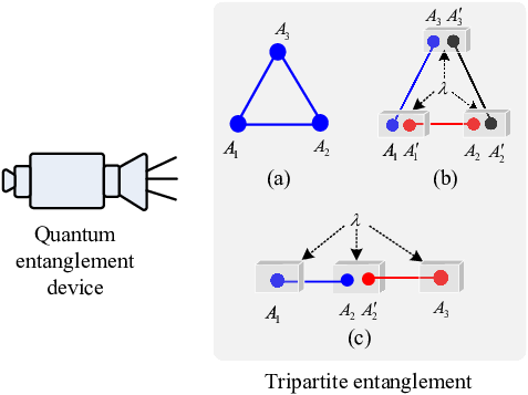
Figure 1: (Color online) Tripartite entangled systems. (a) GHZ state GHZ. (b) Tripartite entangled system consisting of three EPR states EPR of |ϕ⟩A1​A3,|ϕ⟩A1′​A2|\phi\rangle_{A_{1}A_{3}},|\phi\rangle_{A_{1}^{\prime}A_{2}} and |ϕ⟩A2′​A3′|\phi\rangle_{A_{2}^{\prime}A_{3}^{\prime}}. It can be regarded as a high-dimensional entangled state of |Φ⟩=12​2​(|000⟩+|012⟩+|120⟩+|132⟩+|201⟩+|213⟩+|321⟩+|333⟩)A1​A1′,A2​A2′,A3​A3′|\Phi\rangle=\frac{1}{2\sqrt{2}}(|000\rangle+|012\rangle+|120\rangle+|132\rangle+|201\rangle+|213\rangle+|321\rangle+|333\rangle)_{A_{1}A_{1}^{\prime},A_{2}A_{2}^{\prime},A_{3}A_{3}^{\prime}} on Hilbert space ℂ4⊗ℂ4⊗ℂ4\mathbb{C}^{4}\otimes\mathbb{C}^{4}\otimes\mathbb{C}^{4}. (c) Tripartite entangled system consisting of two EPR states |ϕ⟩A1​A2|\phi\rangle_{A_{1}A_{2}} and |ϕ⟩A2′​A3|\phi\rangle_{A_{2}^{\prime}A_{3}}. It is equivalent to an unbalanced high-dimensional entanglement of |Ψ⟩=12​(|000⟩+|011⟩+|120⟩+|131⟩)A1,A2​A2′,A3|\Psi\rangle=\frac{1}{2}(|000\rangle+|011\rangle+|120\rangle+|131\rangle)_{A_{1},A_{2}A_{2}^{\prime},A_{3}} on Hilbert space ℂ2⊗ℂ4⊗ℂ2\mathbb{C}^{2}\otimes\mathbb{C}^{4}\otimes\mathbb{C}^{2}. The schematic encoding for local two-qubit system is defined according to an isomorphism mapping from Hilbert space ℍAi⊗ℍAi′\mathbb{H}_{A_{i}}\otimes\mathbb{H}_{A_{i}^{\prime}} to ℂ4\mathbb{C}^{4} as: ℱ:|00⟩↦|0⟩,|01⟩↦|1⟩,|10⟩↦|2⟩,|11⟩↦|3⟩{\cal F}:|00\rangle\mapsto|0\rangle,|01\rangle\mapsto|1\rangle,|10\rangle\mapsto|2\rangle,|11\rangle\mapsto|3\rangle, where ℍAi\mathbb{H}_{A_{i}} and ℍAi′\mathbb{H}_{A_{i}^{\prime}} are the respective state space of AiA_{i} and Ai′A_{i}^{\prime}. All parties are allowed to perform local operations which may depend on any shared randomness λ\lambda in a LHV model.

Despite of these improvements on single entangled systems and quantum networks, there is no result to distinguish single entangled systems from these being constructed by quantum networks and shared randomness. Note that classical communication is an important resource in the entanglement swapping ZZH. However, it is not allowed for communicating local measurements with each other during Bell experiments except for the final statistics EPR; Bell; BGP; RBB; Chav; Luo. Otherwise, the nonlocal correlations can be forged by using shared randomness and classical communication TB. This difference implies distinctive features for various entangled systems. One intuitive example is shown in Fig.1. All the quantum states are genuinely tripartite entangled in the biseparable model Sy by using recent method ZDBS, where any two parties can generate an EPR state assisted by LOCC of other parties. Surprisingly, they are inequivalent under local operations without classical communication. Actually, the Greenberger-Horne-Zeilinger (GHZ) state |G​H​Z⟩=12​(|000⟩+|111⟩)|GHZ\rangle=\frac{1}{\sqrt{2}}(|000\rangle+|111\rangle) shown in Fig.1(a) is permutationally symmetric, i.e., the density operator is invariant under any permutation of three particles. The total system of the tripartite cyclic network shown in Fig.1(b) is equivalent to an 44-dimensional entanglement of |Φ⟩=12​2​(|000⟩+|012⟩+|120⟩+|132⟩+|201⟩+|213⟩+|321⟩+|333⟩)A1​A1′,A2​A2′,A3​A3′|\Phi\rangle=\frac{1}{2\sqrt{2}}(|000\rangle+|012\rangle+|120\rangle+|132\rangle+|201\rangle+|213\rangle+|321\rangle+|333\rangle)_{A_{1}A_{1}^{\prime},A_{2}A_{2}^{\prime},A_{3}A_{3}^{\prime}} under local operations, which is invariant under the cyclic permutation of joint systems A1​A1′,A2​A2′A_{1}A_{1}^{\prime},A_{2}A_{2}^{\prime} and A3​A3′A_{3}A_{3}^{\prime} Gisin2; RBBB. However, the total system of the tripartite chain-shaped network shown in Fig.1(c) is equivalent to the entanglement of |Ψ⟩=12​(|000⟩+|011⟩+|120⟩+|131⟩)A1,A2​A2′,A3|\Psi\rangle=\frac{1}{2}(|000\rangle+|011\rangle+|120\rangle+|131\rangle)_{A_{1},A_{2}A_{2}^{\prime},A_{3}} under local operations, which is only invariant under the permutation of A1A_{1} and A3A_{3}. Both |Φ⟩|\Phi\rangle and |Ψ⟩|\Psi\rangle can be regarded as special cluster states Cluster; SAS. GHZ state in Fig.1(a) cannot be generated by |Φ⟩|\Phi\rangle in Fig.1(b) or |Ψ⟩|\Psi\rangle in Fig.1(c) by using local unitary operations. These features imply different nonlocalities in different local models GHZ; BGP; RBBB. Unfortunately, it is unknown how to characterize this difference for generally entangled states.

In this work, we propose an approach to investigate new features of single multipartite entangled systems going beyond multisource quantum networks Mayer. The main idea is to verify that some nn-partite entangled systems with n≥3n\geq 3 cannot be generated by using any quantum networks consisting of at most n−1n-1-partite entangled states. We firstly propose a new local model for describing any state that can be generated by local operations on some quantum network consisting of at most n−1n-1-partite entangled states and shared randomness without classical communication. Note that some entangled states in the biseparable model Sy such as examples in Fig.1(b) and (c) are not entangled in the present model. This means that the present model is stronger than the biseparable model Sy, where all the biseparable states are not entangled in the present local model. We further prove that all the permutationally symmetric nn-partite entangled pure states such as GHZ states GHZ, W state Dicke1 and Dicke states Toth are new genuinely multipartite entangled in the present local model. This shows new genuinely multipartite nonlocality going beyond its verified by using the biseparable model Sy or network model with multiple independent sources RBBB; CASA. Moreover, we show that similar result holds for any multipartite entangled pure states in the biseparable model Sy when all the dimensions of local systems are no more than 3. Finally, we provide a useful method to verify noisy states. These results show distinctive features of single multipartite entangled systems going beyond previous local models Sy; GHZ; Cluster; SAS; GS.

II Results

II.1 New local model

In this section, we propose a method to verify single entangled systems in a new local model going beyond the biseparable model Sy. This is also interesting in fully device-independent quantum information processing Mayer; SCAK; AGC; UV, where entanglement devices may be provided by an adversary.

Consider an nn-partite state ρ\rho on Hilbert space ⊗i=1nℍAi\otimes_{i=1}^{n}\mathbb{H}_{A_{i}}, where ℍAi\mathbb{H}_{A_{i}} has local dimension did_{i} with di≥2d_{i}\geq 2, i=1,⋯,ni=1,\cdots,n. We define a new local model as follows.
Refer to caption
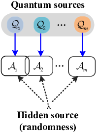
Figure 2: (Color online) Schematic local model of quantum states with distributed settings. Each quantum entangled source 𝒬i{\cal Q}_{i} is shared at most n−1n-1 parties 𝒜i={As1,⋯,Asi}{\cal A}_{i}=\{\textsf{A}_{s_{1}},\cdots,\textsf{A}_{s_{i}}\}, i=1,⋯,mi=1,\cdots,m. All the parties A1,⋯,An\textsf{A}_{1},\cdots,\textsf{A}_{n} can share a hidden randomness λ\lambda.

Definition 1. ρ\rho is new genuinely multipartite entanglement if it cannot be decomposed into a quantum network state as

ρ\displaystyle\rho =\displaystyle= ∑λp(λ)ℰ1(λ)⊗⋯⊗ℰn(λ)(ρ1⊗⋯⊗ρm)\displaystyle\sum_{\lambda}p(\lambda){\cal E}_{1}(\lambda)\otimes\cdots\otimes{\cal E}_{n}(\lambda)(\rho_{1}\otimes\cdots\otimes\rho_{m})
=\displaystyle= ∑λp(λ)∑i,j⊗j=1nUi,j(λ)(ρ1⊗⋯⊗ρm)(⊗j=1nUi,j(λ)†)\displaystyle\sum_{\lambda}p(\lambda)\sum_{i,j}\otimes_{j=1}^{n}U_{i,j}(\lambda)(\rho_{1}\otimes\cdots\otimes\rho_{m})(\otimes_{j=1}^{n}U_{i,j}(\lambda)^{\dagger})

where ρ1,⋯,ρm\rho_{1},\cdots,\rho_{m} are entangled states shared at most n−1n-1 parties, {p⁡(λ)}\{p(\lambda)\} is a distribution of random variable λ\lambda, and ℰi​(λ){\cal E}_{i}(\lambda) is a completely positive trace-preserving (CPTP mapping) GC depending on one shared measurable variable λ\lambda performed by the ii-th party, which can be further represented by Kraus operators Ui,j​(λ)U_{i,j}(\lambda) with ∑jUi,j​(λ)​Ui,j​(λ)†=𝟙\sum_{j}U_{i,j}(\lambda)U_{i,j}(\lambda)^{\dagger}=\mathbbm{1}, 𝟙\mathbbm{1} denotes the identity operator, i=1,⋯,ni=1,\cdots,n. Here, Ui,j​(λ)U_{i,j}(\lambda) are quantum operations that are physically realizable without classical communication.

The classical communication is not allowed in the present local model, i.e., all the local parties cannot communicate their local operations during the process of state generation. The reason is as follows. For any two entangled pure states |Φ0⟩|\Phi_{0}\rangle and |Φ1⟩|\Phi_{1}\rangle on the same Hilbert space ℍ\mathbb{H}, we can prove that they are equivalent under LOCC assisted by teleportation-based quantum computation GC, even if |Φ0⟩|\Phi_{0}\rangle and |Φ1⟩|\Phi_{1}\rangle have different nonlocalities in different local models GHZ; BGP; RBBB.

Take the state shown in Fig.1(b) as an example. The total system has the decomposition in Eq.() with three bipartite entangled pure states. Moreover, the total system in Fig.1(c) has the decomposition in Eq.() with two bipartite entangled pure states. Interestingly, GHZ state shown in Fig.1(a) cannot be generated according to the distributed settings in Fig.1(b) or Fig.1(c) without classical communication. It will be formally proved in Theorem 1.

Consider a general state ρ\rho on Hilbert space ⊗i=1nℍAi\otimes_{i=1}^{n}\mathbb{H}_{A_{i}}. If ρ\rho is a genuinely nn-partite entanglement in the biseperable model Sy, it cannot be decomposed into the biseparable state as

ρ=∑I1,I2∑ipi​ρi(I1)⊗ρi(I2)\displaystyle\rho=\sum_{I_{1},I_{2}}\sum_{i}p_{i}\rho^{(I_{1})}_{i}\otimes{}\rho^{(I_{2})}_{i} (2)

where {I1,I2}\{I_{1},I_{2}\} is a bipartite partition of {A1,⋯,An}\{A_{1},\cdots,A_{n}\}, i.e., I1∪I2={A1,⋯,An}I_{1}\cup{}I_{2}=\{A_{1},\cdots,A_{n}\} and I1∩I2=∅I_{1}\cap I_{2}=\varnothing, and ρi(Ij)\rho^{(I_{j})}_{i} are density operators of local system IjI_{j}, j=1,2j=1,2. From Eq.(2), it is easy to prove that the total states shown in Fig.1(b) and (c) are genuinely tripartite entangled states in the biseperable model Sy. However, they are not new genuinely multipartite entangled in the local model given in Eq.(). This means that the present multipartite entanglement from Definition 1 is stronger than its verified by using the biseperable model Sy given in Eq.(2).

Generally, consider an nn-partite quantum network as shown in Fig.2. Each entangled source 𝒬j{\cal Q}_{j} is shared by ℓi\ell_{i} parties 𝒜i={As1,⋯,Asℓi}{\cal A}_{i}=\{\textsf{A}_{s_{1}},\cdots,\textsf{A}_{s_{\ell_{i}}}\} with 1≤ℓi<n1\leq\ell_{i}<n. The present local model in Eq.() allows local quantum operations depending on any measurable variable λ\lambda Bu. This is different from the non-multilocality BGP; RBB; Chav; Luo and genuinely tripartite nonlocality Fri; Gisin2; RBBB with the assumption of multiple independent randomness shared by all parties. Unfortunately, previous Bell-type inequalities BCM; BCPS or witness operators HHH are difficult to verify the new genuinely multipartite entangled systems.

II.2 New genuinely multipartite entanglement

Our goal in this section is to explore new genuinely entangled states in the local model given in Eq.(). Similar to the examples in Fig.1, we will prove that the lack of symmetry is actually generic for all the states with decompositions in Eq.(). An nn-partite state is permutationally symmetric if its density operator ρ\rho is invariant under any permutation operation 𝗀∈𝕊n\mathsf{g}\in\mathbb{S}_{n}, where 𝕊n\mathbb{S}_{n} denotes the permutation group associated with a set of nn different elements.

One example is generalized dd-dimensional GHZ state GHZ; Cere defined by

|GHZ⟩=∑i=0d−1ai|i⋯i⟩A1⋯An\displaystyle|GHZ\rangle=\sum_{i=0}^{d-1}a_{i}|i\cdots{}i\rangle_{A_{1}\cdots{}A_{n}} (3)

on Hilbert space ⊗i=1nℍAi\otimes_{i=1}^{n}\mathbb{H}_{A_{i}}, where ℍAi\mathbb{H}_{A_{i}}s have the same local dimension dd with d≥2d\geq 2, and aia_{i}s satisfy ∑i=0d−1ai2=1\sum_{i=0}^{d-1}a_{i}^{2}=1.

Another example is generalized Dicke state Toth (including W state as a special example Dicke1) given by

|Dk,n⟩=1Nk,n∑i1+⋯+in=k|i1⋯in⟩A1⋯An\displaystyle|D_{k,n}\rangle=\frac{1}{\sqrt{N_{k,n}}}\sum_{i_{1}+\cdots{}+i_{n}=k}|i_{1}\cdots{}i_{n}\rangle_{A_{1}\cdots{}A_{n}} (4)

where Nk,n=C⁡(k+n−1,n−1)N_{k,n}=C(k+n-1,n-1) denotes the combination number of choosing n−1n-1 balls from a box with k+n−1k+n-1 balls, k=1,⋯,n​d−d−1k=1,\cdots,nd-d-1. Dicke states are very interesting because of the robustness against the particle loss, global dephasing, and bit flip noise Dicke2. These states are genuinely multipartite entangled DPR; Dicke4; TDS in the biseparable model Sy given in Eq.(2). They are also different from cluster states Cluster or stabilize states HEB. Generally, any permutationally symmetric pure state can be represented by the superposition of Dicke states. All the permutationally symmetric entangled pure states can be verified using Hardy-type inequalities CYZ in the biseparable model Sy. Here, we show that they are new genuinely entangled states in the present model in Definition 1.

Theorem 1. Any nn-partite (n≥3n\geq 3) permutationally symmetric entangled pure state in the biseparable model is new genuinely nn-partite entanglement in the local model given in Eq.(), i.e., it cannot be generated by using mm-partite entangled states with m<nm<n under local operations and shared randomness.

The product state |ϕ⟩⊗n|\phi\rangle^{\otimes n}, which is permutationally symmetric, is excluded in Theorem 1.

To show the main idea of proof, we take 44-dimensional permutationally symmetric entangled state |G⟩=12​∑i=03|i​i​i⟩A1​B1​C1|G\rangle=\frac{1}{2}\sum_{i=0}^{3}|iii\rangle_{A_{1}B_{1}C_{1}} as an example. Here, all the 44-dimensional basis states of A1A_{1} (B1B_{1}, or C1C_{1}) can be represented by two qubits A11A_{11} and A12A_{12} (B11B_{11} and B12B_{12}, or C11C_{11} and C12C_{12}) according to the inverse mapping of ℱ{\cal F} defined in Fig.1, where ℍA1=ℍA11⊗ℍA12\mathbb{H}_{A_{1}}=\mathbb{H}_{A_{11}}\otimes\mathbb{H}_{A_{12}}, ℍB1=ℍB11⊗ℍB12\mathbb{H}_{B_{1}}=\mathbb{H}_{B_{11}}\otimes\mathbb{H}_{B_{12}} and ℍC1=ℍC11⊗ℍC12\mathbb{H}_{C_{1}}=\mathbb{H}_{C_{11}}\otimes\mathbb{H}_{C_{12}}. Similar to Eq.(), if |G⟩|G\rangle can be decomposed into two states under the local operations WiW_{i}, we can prove that |G⟩|G\rangle is actually decomposed into two tripartite GHZ states |G1⟩=12​(|000⟩+|111⟩)|G_{1}\rangle=\frac{1}{\sqrt{2}}(|000\rangle+|111\rangle) and |G2⟩=12​(|000⟩+|111⟩)|G_{2}\rangle=\frac{1}{\sqrt{2}}(|000\rangle+|111\rangle), i.e., (W1⊗W2⊗W3)​|G⟩=|G1⟩A11​B11​C11​|G2⟩A12​B12​C12(W_{1}\otimes{}W_{2}\otimes{}W_{3})|G\rangle=|G_{1}\rangle_{A_{11}B_{11}C_{11}}|G_{2}\rangle_{A_{12}B_{12}C_{12}}. Moreover, one of |G1⟩|G_{1}\rangle and |G2⟩|G_{2}\rangle (|G1⟩|G_{1}\rangle for example) is also tripartite entangled in the biseparable model Sy. Note that a 2-dimensional Hilbert space cannot be further decomposed into the tensor of two Hilbert spaces with at least two dimensions. This implies that |G1⟩|G_{1}\rangle cannot be further decomposed into two states. So, there is a tripartite entanglement in the biseparable model Sy after decomposing |G⟩|G\rangle under any local operations. It means that |G⟩|G\rangle must be generated by some states |Ψ1⟩,⋯,|Ψm⟩|\Psi_{1}\rangle,\cdots,|\Psi_{m}\rangle satisfying that one of |Ψi⟩|\Psi_{i}\rangles is a tripartite entanglement in the biseparable model Sy. |G⟩|G\rangle has no decomposition in Eq.() under the local operations.

Generally, for any nn-partite (n≥3n\geq 3) permutationally symmetric entangled pure state |Φ⟩|\Phi\rangle in the biseparable model Sy, we prove that there is an nn-partite entanglement after any decomposition of |Φ⟩|\Phi\rangle under local operations. It means that |Φ⟩|\Phi\rangle must be generated by some states |Ψ1⟩,⋯,|Ψm⟩|\Psi_{1}\rangle,\cdots,|\Psi_{m}\rangle under local operations and shared randomness, where one of |Ψi⟩|\Psi_{i}\rangles is an nn-partite entanglement in the biseparable model Sy. Hence, |Φ⟩|\Phi\rangle has no decomposition in Eq.(), where all the decomposed states are at most n−1n-1-partite entanglement in the biseparable model Sy. The detailed proof of Theorem 1 is shown in Supplementary A.

Theorem 1 implies that any multipartite permutationally symmetric entangled pure state shows a new kind of nn-partite nonlocality. It is well-known that LOCC cannot increase the entanglement of states HHH. Our result shows a further feature of classical communication for distinguishing single entangled systems from these generated by distributed settings without classical communication, even if these states may be equivalent under LOCC (see examples in Fig.1). The new genuinely multipartite entangled systems may have special symmetry under local unitary operations GHZ; Cere; Toth; Dicke1; Dicke2. Interestingly, there are general systems that are also new genuinely multipartite entangled in the local model given in Eq.().

Theorem 2. Any nn-partite (n≥3n\geq 3) entangled pure state on Hilbert space ⊗i=1nℍAi\otimes_{i=1}^{n}\mathbb{H}_{A_{i}} in the biseparable model in Eq.(2) is new genuinely nn-partite entanglement in the local model given in Eq.() if the dimension of ℍAi\mathbb{H}_{A_{i}} is no larger than 33, i=1,⋯,ni=1,\cdots,n.

The proof of Theorem 2 is shown in Supplementary B. The main idea is that each Hilbert space ℍ\mathbb{H} with local dimension d≤3d\leq 3 cannot be decomposed into the tensor of two Hilbert spaces ℍ1\mathbb{H}_{1} and ℍ2\mathbb{H}_{2} with at least two dimensions (even if under the isomorphism mappings). Theorem 2 is important for hybrid systems whose local particles have different state spaces KBK. Theorems 1 and 2 show general results of new genuinely multipartite entanglement in the present model given in Eq.(). A directive result is for any pure state being equivalent to one entangled state in Theorem 1 or 2 using local unitary operations and auxiliary states.
Refer to caption
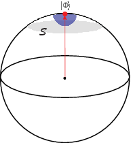
Figure 3: (Color online) Schematic entangled states on Bloch sphere. The red dot denotes the pure state |Φ⟩|\Phi\rangle. |Φ⟩|\Phi\rangle is a new genuinely nn-partite entangled in the local model given in Eq.(). The grey hyperplane 𝒮{\cal S} is defined by all the network states ρn​e​t\rho_{net} defined in Eq.() with F⁡(ρn​e​t,|Φ⟩)=D⁡(|Φ⟩)F(\rho_{net},|\Phi\rangle)=D(|\Phi\rangle), where D⁡(|Φ⟩)D(|\Phi\rangle) and F⁡(ρn​e​t,|Φ⟩)F(\rho_{net},|\Phi\rangle) are defined in Eq.(5). All the states above the grey hyperplane are new genuinely multipartite entangled in the local model given in Eq.().

II.3 New genuinely multipartite entanglement with noises

In this section, we will prove that the present new genuinely multipartite entanglement is robust against general noises. For an nn-partite pure state on Hilbert space ⊗i=1nℍAi\otimes_{i=1}^{n}\mathbb{H}_{A_{i}}, inspired by the biseparable model Sy; HHH, denote D⁡(|Φ⟩)D(|\Phi\rangle) as the maximal distance between |Φ⟩|\Phi\rangle and all the network states ρn​e​t\rho_{net} defined in Eq.(), i.e.,

D⁡(|Φ⟩)=supρn​e​tF⁡(ρn​e​t,ρΦ)\displaystyle D(|\Phi\rangle)=\sup_{\rho_{net}}F(\rho_{net},\rho_{\Phi}) (5)

where ρΦ\rho_{\Phi} denotes the density operator defined by ρΦ=|Φ⟩​⟨Φ|\rho_{\Phi}=|\Phi\rangle\langle\Phi|, F⁡(ρ,ρΦ)=(tr⁡(|Φ⟩​⟨Φ|​ρ))2F(\rho,\rho_{\Phi})=({\rm tr}(|\Phi\rangle\langle\Phi|\sqrt{\rho}))^{2} denotes the fidelity between ρ\rho and ρΦ\rho_{\Phi} Jozsa. It is easy to get that F⁡(ρn​e​t,ρΦ)≤maxi⁡|⟨Φ|Ψi⟩|2F(\rho_{net},\rho_{\Phi})\leq\max_{i}|\langle\Phi|\Psi_{i}\rangle|^{2} if ρn​e​t\rho_{net} has the decomposition of ρn​e​t=∑ipi​|Ψi⟩​⟨Ψi|\rho_{net}=\sum_{i}p_{i}|\Psi_{i}\rangle\langle\Psi_{i}|. Hence, it is sufficient to evaluate D⁡(|Φ⟩)D(|\Phi\rangle) by considering all the pure states with the decompositions in Eq.() as

D(|Φ⟩)=sup⊗i=1m|Ψi⟩|⟨Φ|⊗j=1nUj(⊗i=1m|Ψi⟩)|2\displaystyle D(|\Phi\rangle)=\sup_{\otimes_{i=1}^{m}|\Psi_{i}\rangle}|\langle\Phi|\otimes_{j=1}^{n}U_{j}(\otimes_{i=1}^{m}|\Psi_{i}\rangle)|^{2} (6)

where |Ψi⟩|\Psi_{i}\rangle is any nn-partite states with at most n−1n-1 particles being entangled, UiU_{i} is an arbitrary local unitary operation performed by the ii-th party, i=1,⋯,ni=1,\cdots,n.

From the compactness of Bloch sphere, using the present model given in Eq.() we get

D⁡(|Φ⟩)<1\displaystyle D(|\Phi\rangle)<1 (7)

for any new genuinely multipartite entangled state |Φ⟩|\Phi\rangle. From Fig.3, we get a sufficient condition for witnessing a new genuinely multipartite entangled state ρ\rho in the local model given in Eq.() if

F⁡(ρ,ρΦ)>D⁡(|Φ⟩)\displaystyle F(\rho,\rho_{\Phi})>D(|\Phi\rangle) (8)

Note that from the convexity of fully separable states or biseparable states Sy; HHH, there is a witness operator HHH; Chru for verifying each entanglement apart from fully separable states, or each genuinely multipartite entanglement in the biseparable model Sy. Interestingly, all the states defined in Eq.() consist of a convex set. Hence, the condition in Eq.(8) implies a new witness operator HHH; Chru as

𝒲=F⁡(ρ,ρΦ)​𝕀−|Φ⟩​⟨Φ|\displaystyle{\cal W}=F(\rho,\rho_{\Phi})\mathbb{I}-|\Phi\rangle\langle\Phi| (9)

in order to separate a multipartite state ρ\rho from all the network states defined in Eq.(), i.e., we get from Eqs.(6)-(8) that

tr⁡[𝒲​ρn​e​t]≥0\displaystyle{\rm tr}[{\cal W}\rho_{net}]\geq 0 (10)

for all the network states ρn​e​t\rho_{net} defined in Eq.(), and

tr⁡[𝒲​ϱ]<0\displaystyle{\rm tr}[{\cal W}\varrho]<0 (11)

In applications, it is sufficient to choose a specific multipartite entangled pure state |Φ⟩|\Phi\rangle in the local model given, which closes to ϱ\varrho.

Although it is difficult to evaluate D⁡(|Φ⟩)D(|\Phi\rangle) for general states, we provide some sufficient conditions for entangled states in Theorems 1 and 2. Define a generalized permutationally symmetric entanglement as

|Φp​s⟩=∑i=0n​d−n−1αi​|Di,n⟩\displaystyle|\Phi_{ps}\rangle=\sum_{i=0}^{nd-n-1}\alpha_{i}|D_{i,n}\rangle (12)

where |D0,n⟩:=β0​|0⟩⊗n+β1​|d−1⟩⊗n|D_{0,n}\rangle:=\beta_{0}|0\rangle^{\otimes n}+\beta_{1}|d-1\rangle^{\otimes n} with β02+β12=1\beta_{0}^{2}+\beta_{1}^{2}=1, and |Dk,n⟩|D_{k,n}\rangle is Dicke states defined in Eq.(4). Here, special restrictions of αi\alpha_{i}s should be imposed to exclude symmetric product states. Generally, we prove the following result.

Theorem 3. For any nn-partite (n≥3n\geq 3) state ρ\rho on Hilbert space ⊗i=1nℍAi\otimes_{i=1}^{n}\mathbb{H}_{A_{i}}, it is new genuinely entangled in the model given in Eq.() if one of the following facts holds

  • (i)

    For generalized GHZ state |G​H​Z⟩|GHZ\rangle defined in Eq.(3), ρ\rho satisfies

    F⁡(ρ,ρG​H​Z)>max⁡{a02,⋯,ad−12}\displaystyle F(\rho,\rho_{GHZ})>\max\{a^{2}_{0},\cdots,a^{2}_{d-1}\} (13)
  • (ii)

    For Dicke state |Dk,n⟩|D_{k,n}\rangle defined in Eq.(4), ρ\rho satisfies

    F⁡(ρ,ρDk,n)\displaystyle F(\rho,\rho_{D_{k,n}}) =\displaystyle= F⁡(ρ,ρDn​d−n−k−1,n)\displaystyle F(\rho,\rho_{D_{nd-n-k-1,n}}) (14)
    >\displaystyle> n−1n+k−1\displaystyle\frac{n-1}{n+k-1}

    for k=1,⋯,⌊n​d−n−12⌋k=1,\cdots,\lfloor\frac{nd-n-1}{2}\rfloor, where ⌊x⌋\lfloor{}x\rfloor denotes the maximal integer no larger than xx.

  • (iii)

    For |Φp​s⟩|\Phi_{ps}\rangle defined in Eq.(12), ρ\rho satisfies

    F⁡(ρ,ρΦp​s)\displaystyle F(\rho,\rho_{\Phi_{ps}}) >\displaystyle> ∑i=1⌊n​d−n−12⌋n−1n+i−1​(αi2+αn​d−n−1−i2)\displaystyle\sum_{i=1}^{\lfloor\frac{nd-n-1}{2}\rfloor}\frac{n-1}{n+i-1}(\alpha_{i}^{2}+\alpha_{nd-n-1-i}^{2}) (15)
    +α02​β2\displaystyle+\alpha_{0}^{2}\beta^{2}

    for an odd n​d−n−1nd-n-1; or

    F⁡(ρ,ρΦp​s)\displaystyle F(\rho,\rho_{\Phi_{ps}}) >\displaystyle> ∑i=1⌊n​d−n−12⌋n−1n+i−1​(αi2+αn−i2)\displaystyle\sum_{i=1}^{\lfloor\frac{nd-n-1}{2}\rfloor}\frac{n-1}{n+i-1}(\alpha_{i}^{2}+\alpha_{n-i}^{2}) (16)
    +α02​β2−2​n−2n​d+n−3​αn​d−n−122\displaystyle+\alpha_{0}^{2}\beta^{2}-\frac{2n-2}{nd+n-3}\alpha_{\frac{nd-n-1}{2}}^{2}

    for an even n​d−n−1nd-n-1, where β\beta is given by β=max⁡{β0,β1}\beta=\max\{\beta_{0},\beta_{1}\}.

  • (iv)

    For a new genuinely nn-partite entangled qubit state |Φ⟩|\Phi\rangle in the present model, ρ\rho satisfies

    F⁡(ρ,ρΦ)>max𝒜⊂{A1,⋯,An}⁡max⁡{σ⁡(ρ𝒜)}\displaystyle F(\rho,\rho_{\Phi})>\max_{{\cal A}\subset\{A_{1},\cdots,A_{n}\}}\max\{\sigma(\rho_{\cal A})\} (17)

    where σ⁡(ρ𝒜)\sigma(\rho_{\cal A}) denotes all the eigenvalues of ρ𝒜\rho_{\cal A}, and ρ𝒜\rho_{\cal A} denotes the reduced density matrix ρ𝒜\rho_{\cal A} of the subsystems in 𝒜{\cal A} with 𝒜⊂{A1,⋯,An}{\cal A}\subset\{A_{1},\cdots,A_{n}\}.

Theorem 3 provides a useful method to verify new genuinely multipartite entangled states with general noises in the local model given in Eq.(). The proof of Theorem 3 is given in Supplementary C. The main idea is to evaluate D⁡(|Φ⟩)D(|\Phi\rangle) defined in Eq.(6) for special states |Φ⟩|\Phi\rangle.

II.4 Examples

In this section, we present some examples of new genuinely multipartite entangled states with noises.

Example 1. Consider an nn-partite GHZ state defined in Eq.(3) with white noise as follows Werner:

ρv=v⁡|G​H​Z⟩​⟨G​H​Z|+1−vdn​𝟙dn\displaystyle\rho_{v}=v|GHZ\rangle\langle GHZ|+\frac{1-v}{d^{n}}\mathbbm{1}_{d^{n}} (18)

where 𝟙dn\mathbbm{1}_{d^{n}} denotes the identity operator on Hilbert space ⊗i=1nℍAi\otimes_{i=1}^{n}\mathbb{H}_{A_{i}}, and ℍAi\mathbb{H}_{A_{i}} has the same local dimension dd with d≥2d\geq 2. The weight vv may operationally represent the interferometric contrast observed in experiment Werner. For the maximally entangled GHZ state |G​H​Z⟩|GHZ\rangle with d=2d=2, from Eq.(13), ρv\rho_{v} is new genuinely nn-partite entangled in the local model given in Eq.() for v>2n−1−12n−1v>\frac{2^{n-1}-1}{2^{n}-1}. This is consistent with the genuinely multipartite nonlocality in the biseparable model GS; Sy given in Eq.(2). Moreover, from Eqs.(9)-(11) and Eq.(13), it follows a witness operator as

𝒲G​H​Z=a​𝟙dn−|G​H​Z⟩​⟨G​H​Z|\displaystyle{\cal W}_{GHZ}=a\mathbbm{1}_{d^{n}}-|GHZ\rangle\langle GHZ| (19)

for verifying ρv\rho_{v} in the local model given in Definition 1 when

v≥dn​a−1dn−1\displaystyle v\geq\frac{d^{n}a-1}{d^{n}-1} (20)

where a=max⁡{a02,⋯,ad−12}a=\max\{a^{2}_{0},\cdots,a_{d-1}^{2}\}.

Example 2. Consider a Dicke state defined in Eq.(4) with white noise as follows

ϱv=v⁡|Dk,n⟩​⟨Dk,n|+1−vdn​𝟙dn\displaystyle\varrho_{v}=v|D_{k,n}\rangle\langle{}D_{k,n}|+\frac{1-v}{d^{n}}\mathbbm{1}_{d^{n}} (21)

where v∈[0,1]v\in[0,1], and k≤⌊n​d−n−12⌋k\leq\lfloor\frac{nd-n-1}{2}\rfloor. From Eqs.(9)-(11) and (14), it provides a witness operator as

𝒲Dk,n=n−1n+k−1​𝟙dn−|Dk,n⟩​⟨Dk,n|\displaystyle{\cal W}_{D_{k,n}}=\frac{n-1}{n+k-1}\mathbbm{1}_{d^{n}}-|D_{k,n}\rangle\langle D_{k,n}| (22)

for verifying new genuinely nn-partite entangled ϱv\varrho_{v} in the local model given in Eq.() when vv satisfies

v≥(n−1)​2n−n−k+1(2n−1)​(n+k−1)\displaystyle v\geq\frac{(n-1)2^{n}-n-k+1}{(2^{n}-1)(n+k-1)} (23)

Similarly, we can verify a general permutationally symmetric noisy state ϱv\varrho_{v} defined by

ϱv=∑k=1n​d−n−1vk​|Dk,n⟩​⟨Dk,n|+v0dn​𝟙dn\displaystyle\varrho_{v}=\sum_{k=1}^{nd-n-1}v_{k}|D_{k,n}\rangle\langle{}D_{k,n}|+\frac{v_{0}}{d^{n}}\mathbbm{1}_{d^{n}} (24)

where vi≥0v_{i}\geq 0 and ∑i=0n​d−n−1vi=1\sum_{i=0}^{nd-n-1}v_{i}=1. One method is from Eq.(22). Define an operator 𝒲D,n{\cal W}_{D,n} as

𝒲D,n=∑k=1n​d−n−1𝒲Dk,n\displaystyle{\cal W}_{D,n}=\sum_{k=1}^{nd-n-1}{\cal W}_{D_{k,n}} (25)

It is forward to prove that 𝒲D,n{\cal W}_{D,n} is a useful witness operator from Eqs.(9)-(11) when v0v_{0} satisfies the following inequality

v0<dndn−n​d+n+1​(1−∑k=1n​d−n−1Lk)\displaystyle v_{0}<\frac{d^{n}}{d^{n}-nd+n+1}(1-\sum_{k=1}^{nd-n-1}L_{k}) (26)

where Lk=Ln​d−n−1−k=n−1n+k−1L_{k}=L_{nd-n-1-k}=\frac{n-1}{n+k-1} for k=1k=1, ⋯\cdots, ⌊n​d−n−12⌋\lfloor\frac{nd-n-1}{2}\rfloor.

Another way for verifying ϱv\varrho_{v} in Eq.(24) is using permutationally symmetric state |Φp​s⟩|\Phi_{ps}\rangle defined in Eq.(12). In fact, from Eq.(15), it is easy to construct a witness operator 𝒲Φp​s{\cal W}_{\Phi_{ps}} for verifying ϱv\varrho_{v} in the local model given in Eq.() as

𝒲Φp​s\displaystyle{\cal W}_{\Phi_{ps}} =\displaystyle= (∑i=1⌊n​d−n−12⌋n−1n+i−1​(αi2+αn​d−n−1−i2)CLOSE\displaystyle(\sum_{i=1}^{\lfloor\frac{nd-n-1}{2}\rfloor}\frac{n-1}{n+i-1}(\alpha_{i}^{2}+\alpha_{nd-n-1-i}^{2}) (27)
+α02β2)𝟙dn−|Φp​s⟩Φp​s|\displaystyle\left.+\alpha_{0}^{2}\beta^{2}\right)\mathbbm{1}_{d^{n}}-|\Phi_{ps}\rangle\Phi_{ps}|

when all viv_{i}s satisfy

∑k=1n​d−n−1vk​αk2+v0​α02dn\displaystyle\sum_{k=1}^{nd-n-1}v_{k}\alpha_{k}^{2}+\frac{v_{0}\alpha_{0}^{2}}{d^{n}} >\displaystyle> ∑i=1⌊n​d−n−12⌋n−1n+i−1​(αi2+αn​d−n−1−i2)\displaystyle\sum_{i=1}^{\lfloor\frac{nd-n-1}{2}\rfloor}\frac{n-1}{n+i-1}(\alpha_{i}^{2}+\alpha_{nd-n-1-i}^{2}) (28)
+α02​β2\displaystyle+\alpha_{0}^{2}\beta^{2}

Similar result holds for n​d−n−1nd-n-1 being an even integer from Eq.(16).

Note that the present model given in Eq.() is stronger than the biseperable model in Eq.(2). All the witness operators of 𝒲Dk,n{\cal W}_{D_{k,n}} defined in Eq.(22), 𝒲D,n{\cal W}_{D,n} defined in Eq.(25) and 𝒲Φp​s{\cal W}_{\Phi_{ps}} defined in Eq.(27) are then useful for verifying genuinely multipartite entangled states in the biseparable model Sy.

Example 3. Consider a new genuinely nn-partite entangled pure state |Φ⟩|\Phi\rangle on Hilbert space ⊗i=1nℍAi\otimes_{i=1}^{n}\mathbb{H}_{A_{i}} in the local model given in Eq.(), where did_{i} denotes the dimension of ℍAi\mathbb{H}_{A_{i}}, i=1,⋯,ni=1,\cdots,n. Define a noisy state of |Φ⟩|\Phi\rangle as

ρv=v⁡|Φ⟩​⟨Φ|+(1−v)​ϱ\displaystyle\rho_{v}=v|\Phi\rangle\langle\Phi|+(1-v)\varrho (29)

where ϱ\varrho is a general noisy operator, such as white noise Werner, depolarization BGK, or erasure errors GBP, which should be positive semidefinite with unit trace. Theorem 3 provides an efficient method to verify ρv\rho_{v} in Eq.(29) in the local model given in Eq.(). One method is to use the symmetric space spanned by Dicke states |Dk,n⟩|D_{k,n}\rangle. Especially, by using the witness operator 𝒲D,n{\cal W}_{D,n} defined in Eq.(25), there is a sufficient condition

v>∑k=1n​d−n−1Lk∑k=1n​d−n−1βk\displaystyle v>\frac{\sum_{k=1}^{nd-n-1}L_{k}}{\sum_{k=1}^{nd-n-1}\beta_{k}} (30)

in order to verify a new genuinely nn-partite entangled ρv\rho_{v} in Eq.(29) in the local model given in Eq.(), where βi=|⟨Di,n|Φ⟩|2\beta_{i}=|\langle{}D_{i,n}|\Phi\rangle|^{2} for i=1,⋯,n​d−n−1i=1,\cdots,nd-n-1, and Lk=Ln​d−n−1−k=n−1n+k−1L_{k}=L_{nd-n-1-k}=\frac{n-1}{n+k-1} for k=1,⋯,⌊n​d−n−12⌋k=1,\cdots,\lfloor\frac{nd-n-1}{2}\rfloor.

The second is using the witness operator 𝒲Φp​s{\cal W}_{\Phi_{ps}} defined in Eq.(27) when vv satisfies

v>α02​β2+∑i=1⌊n​d−n−12⌋n−1n+i−1​(αi2+αn​d−n−1−i2)\displaystyle v>\alpha_{0}^{2}\beta^{2}+\sum_{i=1}^{\lfloor\frac{nd-n-1}{2}\rfloor}\frac{n-1}{n+i-1}(\alpha_{i}^{2}+\alpha_{nd-n-1-i}^{2}) (31)

These conditions are also useful for verifying the genuinely multipartite entanglement in the biseparable model Sy.

Another one is using the condition defined in Eq.(17) qubit states, i=1,⋯,3i=1,\cdots,3. Assume that |Φ⟩|\Phi\rangle is given by

|Φ⟩=∑i1⋯inαi1⋯in|i1⋯in⟩\displaystyle|\Phi\rangle=\sum_{i_{1}\cdots i_{n}}\alpha_{i_{1}\cdots i_{n}}|i_{1}\cdots{}i_{n}\rangle (32)

For the bipartition {A1,⋯,Ak}\{A_{1},\cdots,A_{k}\} and {Ak+1,⋯,An}\{A_{k+1},\cdots,A_{n}\} of {A1,⋯,An}\{A_{1},\cdots,A_{n}\}, denote ρA1⋯Ak\rho_{A_{1}\cdots{}A_{k}} as the reduced density matrix on the subsystems {A1,⋯,Ak}\{A_{1},\cdots,A_{k}\}. It follows that HJ:

λmax(ρA1⋯Ak)≤max{∥vi∥1}\displaystyle\lambda_{\max}(\rho_{A_{1}\cdots{}A_{k}})\leq\max\{\|v_{i}\|_{1}\} (33)

where vjv_{j} is the jj-th column vector of ρA1⋯Ak\rho_{A_{1}\cdots{}A_{k}}, and ‖x‖=∑i|xi|\|x\|=\sum_{i}|x_{i}| denotes the 11-norm of vector. This provides an efficient method without evaluating all the eigenvalues of the reduced density matrices. From Eqs.(17) and (39) we obtain a simple witness operator as

𝒲Φ=α𝟙d1⋯dn−|Φ⟩⟨Φ|\displaystyle{\cal W}_{\Phi}=\alpha\mathbbm{1}_{d_{1}\cdots{}d_{n}}-|\Phi\rangle\langle\Phi| (34)

for verifying new genuinely nn-partite entanglement in the local model given in Eq.(), where α=max⁡{‖ρ𝒜‖c}\alpha=\max\{\|\rho_{{\cal A}}\|_{c}\}, and ‖ρ𝒜‖c\|\rho_{{\cal A}}\|_{c} denotes the maximal 11-norm of column vectors in the reduced density matrix ρ𝒜\rho_{{\cal A}} with 𝒜⊂{A1,⋯,An}{\cal A}\subset\{A_{1},\cdots,A_{n}\}, and 𝟙d1⋯dn\mathbbm{1}_{d_{1}\cdots{}d_{n}} denotes the identity operator on ⊗i=1nℍAi\otimes_{i=1}^{n}\mathbb{H}_{A_{i}}. The witness operator 𝒲Φ{\cal W}_{\Phi} implies a sufficient condition as

v>α−tr⁡[ϱ​|Φ⟩​⟨Φ|]1−tr⁡[ϱ​|Φ⟩​⟨Φ|]\displaystyle v>\frac{\alpha-{\rm tr}[\varrho|\Phi\rangle\langle\Phi|]}{1-{\rm tr}[\varrho|\Phi\rangle\langle\Phi|]} (35)

for verifying ρv\rho_{v} being a new genuinely nn-partite entanglement in the present model given in Eq.().

Example 4. Consider a three-qubit entangled pure state as AAC; Sy:

|Φ3⟩A​B​C\displaystyle|\Phi_{3}\rangle_{ABC} =\displaystyle= λ0​|000⟩+λ1​ei​ϕ​|100⟩+λ2​|101⟩\displaystyle\lambda_{0}|000\rangle+\lambda_{1}e^{i\phi}|100\rangle+\lambda_{2}|101\rangle (36)
+λ3​|110⟩+λ4​|111⟩\displaystyle+\lambda_{3}|110\rangle+\lambda_{4}|111\rangle

where ϕ∈[0,π]\phi\in[0,\pi], λi≥0\lambda_{i}\geq 0, and ∑i=04λi2=1\sum_{i=0}^{4}\lambda_{i}^{2}=1. From Theorem 2, |Φ3⟩A​B​C|\Phi_{3}\rangle_{ABC} is a new genuinely nn-partite entanglement in the present model given in Eq.(). With some evaluations (Supplementary D), from Eq.(17) we get that any state ρ\rho is a new genuinely multipartite entanglement in the model given in Eq.() if

F⁡(ρ,ρΦ3)>γ\displaystyle F(\rho,\rho_{\Phi_{3}})>\gamma (37)

where γ=max⁡{γ1,γ2,γ3}\gamma=\max\{\gamma_{1},\gamma_{2},\gamma_{3}\} and γi\gamma_{i} are given by γ1=12+12​(1−4​λ02​λ22−4​λ02​λ32−4​λ02​λ42)1/2\gamma_{1}=\frac{1}{2}+\frac{1}{2}(1-4\lambda_{0}^{2}\lambda_{2}^{2}-4\lambda_{0}^{2}\lambda_{3}^{2}-4\lambda_{0}^{2}\lambda_{4}^{2})^{1/2}, γ2=12+12​(1+4​δ−4​λ02​λ32)1/2\gamma_{2}=\frac{1}{2}+\frac{1}{2}(1+4\delta-4\lambda_{0}^{2}\lambda_{3}^{2})^{1/2}, γ3=12+12​(1+4​δ−4​λ02​λ22)1/2\gamma_{3}=\frac{1}{2}+\frac{1}{2}(1+4\delta-4\lambda_{0}^{2}\lambda_{2}^{2})^{1/2} with δ=2​λ1​λ2​λ3​λ4−λ02​λ42−λ12​λ42−λ22​λ32\delta=2\lambda_{1}\lambda_{2}\lambda_{3}\lambda_{4}-\lambda_{0}^{2}\lambda_{4}^{2}-\lambda_{1}^{2}\lambda_{4}^{2}-\lambda_{2}^{2}\lambda_{3}^{2}.

Now, consider a noisy state as

ρv=v⁡|Φ3⟩​⟨Φ3|+(1−v)​ϱ\displaystyle\rho_{v}=v|\Phi_{3}\rangle\langle\Phi_{3}|+(1-v)\varrho (38)

where |Φ3⟩|\Phi_{3}\rangle is defined in Eq.(36), ϱ\varrho is a general density operator, and v∈[0,1]v\in[0,1]. This state is a special example of the state defined in Eq.(29). From Eqs.(9) and (37) we get a witness operator as

𝒲Φ3=γ​𝟙8−|Φ3⟩​⟨Φ3|\displaystyle{\cal W}_{\Phi_{3}}=\gamma\mathbbm{1}_{8}-|\Phi_{3}\rangle\langle\Phi_{3}| (39)

for verifying ρv\rho_{v} defined in Eq.(38) in the local model given in Eq.(). It provides a sufficient condition as

v>γ−tr⁡[ϱ⁡|Φ3⟩​⟨Φ3|]1−tr⁡[ϱ⁡|Φ3⟩​⟨Φ3|]\displaystyle v>\frac{\gamma-{\rm tr}[\varrho|\Phi_{3}\rangle\langle\Phi_{3}|]}{1-{\rm tr}[\varrho|\Phi_{3}\rangle\langle\Phi_{3}|]} (40)

for witnessing ρv\rho_{v} defined in Eq.(38) in the present model given in Eq.(). Similar result holds for other entangled states from Eq.(37). Of course, the computation complexity of this method depends on the number of involved quantum systems.
Refer to caption
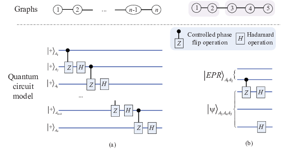
Figure 4: (Color online) Schematic cluster states. (a) nn-qubit GHZ state. (b) Five-qubit linear cluster state. HH denotes Hadamard operation: |0⟩↦|+⟩|0\rangle\mapsto|+\rangle, and |1⟩↦|−⟩|1\rangle\mapsto|-\rangle with |±⟩=12​(|0⟩+|1⟩)|\pm\rangle=\frac{1}{\sqrt{2}}(|0\rangle+|1\rangle). The controlled phase flip operation is given by: |0⟩​⟨0|⊗𝟙+|1⟩​⟨1|⊗σz|0\rangle\langle 0|\otimes\mathbbm{1}+|1\rangle\langle 1|\otimes\sigma_{z}, where σz\sigma_{z} is Pauli operation.

Example 5. Consider cluster states as shown in Fig.4. In Fig.4(a), the final state after all the controlled phase gates is given by

|Φ⟩=12(|0⋯0⟩+|1⋯1⟩)A1⋯An\displaystyle|\Phi\rangle=\frac{1}{\sqrt{2}}(|0\cdots{}0\rangle+|1\cdots{}1\rangle)_{A_{1}\cdots{}A_{n}} (41)

which is an nn-partite GHZ state GHZ. The inequality (20) provides a sufficient condition to verify |Φ⟩|\Phi\rangle with white noise being a new genuinely nn-partite entanglement in the local model given in Eq.().

In Fig.4(b), the final state after all controlled phase gates performed on the joint system of |E​P​R⟩A1​A2​|Ψ⟩A3​A4​A5|EPR\rangle_{A_{1}A_{2}}|\Psi\rangle_{A_{3}A_{4}A_{5}} is given by

|Φ5⟩=12​(a⁡|00000⟩+b⁡|11100⟩+a⁡|00111⟩+b⁡|11011⟩)\displaystyle|\Phi_{5}\rangle=\frac{1}{\sqrt{2}}(a|00000\rangle+b|11100\rangle+a|00111\rangle+b|11011\rangle) (42)

where |Ψ⟩A3​A4​A5|\Psi\rangle_{A_{3}A_{4}A_{5}} is generalized three-qubit linear cluster state given by |Ψ⟩A3​A4​A5=12​(|+⟩​|0⟩​|+⟩+|−⟩​|1⟩​|−⟩)|\Psi\rangle_{A_{3}A_{4}A_{5}}=\frac{1}{\sqrt{2}}(|+\rangle|0\rangle|+\rangle+|-\rangle|1\rangle|-\rangle), and |E​P​R⟩A1​A2|EPR\rangle_{A_{1}A_{2}} denotes the generalized EPR state given by |E​P​R⟩A1​A2=a⁡|00⟩+b⁡|11⟩|EPR\rangle_{A_{1}A_{2}}=a|00\rangle+b|11\rangle with a2+b2=1a^{2}+b^{2}=1. From Theorem 2, this state is a new genuinely 55-partite entangled state in the local model given in Eq.(). Consider the noisy state of ρv\rho_{v} defined in Eq.(29) with |Φ⟩=|Φ5⟩|\Phi\rangle=|\Phi_{5}\rangle and white noise ϱ=132​𝟙32\varrho=\frac{1}{32}\mathbbm{1}_{32}. From the inequality (35) we get a sufficient condition of v≥16​a2−131v\geq\frac{16a^{2}-1}{31} (a≥12a\geq\frac{1}{\sqrt{2}}) for witnessing ρv\rho_{v} in the present model given in Eq.().

Generally, the inequality (35) is useful for verifying the cluster states or graph states Cluster associated with specific graphs. These states are interesting in quantum information processing and measurement-based quantum computations Cluster; NMDB. It is known that single connected graph states have the genuinely multipartite nonlocalities in the biseparable model GTHB; Sy. Theorems 2 and 3 imply new generic nonlocality for the connected graph states with qubit states as inputs in the present model given in Eq.().
Refer to caption
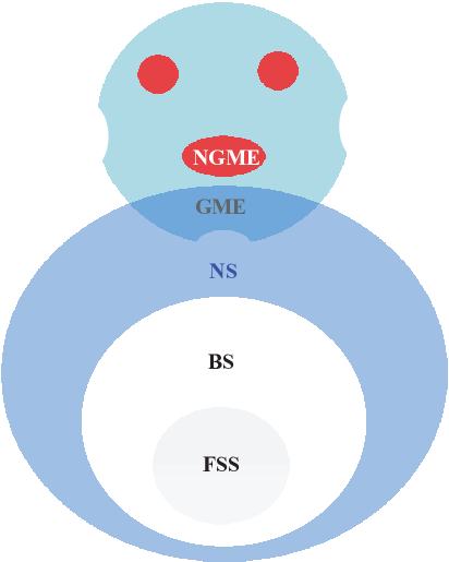
Figure 5: (Color online) Schematic relations of different states. The new genuinely multipartite entanglement (NGME) is stronger than previous genuinely multipartite entanglement (GME) verified by using the biseparable model Sy. NS denotes network state defined in Eq.(). BS denotes states biseparable state in the biseparable model Sy. FSS denotes fully separable state. NGMEs (in red area) are genuinely multipartite entangled states in the biseparable model Sy. The converse is not right, see Fig.1(b) and (c) in the main text. BSs are network states defined in Eq.(). The converse is not right, see Fig.1(b) and (c).

Discussion

The present model given in Eq.() is derived from the distributed settings of entanglement generations ZZH; Kim. All the entangled states that have the decompositions in Eq.() are not symmetric from Theorem 1. This geometric feature has a strong restriction on the resultant from a generation procedure based on quantum networks TDS without classical communication. Interestingly, this shows a new kind of genuinely multipartite entanglement going beyond its verified by all the previous local models Bell; GHZ; Sy. Specially, the present model in Eq.() is stronger than the previous biseparable model Sy that is used to verify the genuinely multipartite entanglement, as shown in Fig.5. It means that all the new genuinely multipartite entangled states in the present model in Definition 1 are genuinely multipartite entangled states in the biseparable model Sy. The converse is not right, see examples in Fig.1(b) and (c). Theorem 1 presents some interesting examples includes all the generalized GHZ states, Dicke states, and generalized permutationally symmetric entangled pure states which are new genuinely multipartite entangled states in the present model.

Similar results hold for other entangled pure states in the biseparable model Sy with small dimensions of local systems from Theorem 2. This means that the present model in Eq.() can verify the same kind of entangled pure states with the biseparable model Sy. Although there are proper isomorphism transformations by local parties for embedding a small state space into a large Hilbert space with the tensor decomposition, however, these local operations are useless for generating specific entangled systems without classical communication. This fact cannot be extended for high-dimensional systems, see examples in Fig.1(b) and (c). Generally, there are lots of multipartite high-dimensional states which have different features in the present model in Eq.() and the biseparable model Sy. So, an interesting problem is how to feature these high-dimensional systems with the present local model. One possible solution is to explore the entangled pure states with prime dimensions of local systems. Another problem is how to verify the entangled states that are generated from new genuinely multipartite entangled states in the present model by using Bell-type inequalities.

Theorem 3 provides a useful method for verifying new genuinely multipartite entanglement in the present local model by using witness operators HHH; Chru. Similar to the biseparable model Sy, all the states with the decompositions in Eq.() consist of a convex set. This feature implies another application of witness operator HHH; Chru. In applications, the state tomography will be performed to find proper entangled pure state for constructing witness operator from Theorem 3. Another method is to find an entangled mixed state which closes to the verified state. Generally, we may define a witness operator for verifying ρ\rho as

𝒲ρ=ζ​𝟙−ρ\displaystyle{\cal W}_{\rho}=\zeta\mathbbm{1}-\rho (43)

where ζ=supρn​e​t(tr⁡[ρn​e​t​ρ​ρn​e​t])2\zeta=\sup_{\rho_{net}}({\rm tr}[\sqrt{\rho_{net}}\sqrt{\rho}\sqrt{\rho_{net}}])^{2} Jozsa and ρn​e​t\rho_{net} is any network state defined in Eq.(). Unfortunately, it is difficult to evaluate ζ\zeta for general states. Hence, an interesting problem is how to compute ζ\zeta for special states.

The present Theorems 1 and 3 are useful for featuring permutationally symmetric entangled states. Actually, there is a standard Bell method to verify some of these entangled states. Especially, we show that all the biseparable states ρ\rho given in Eq.(2) on Hilbert space ⊗i=1nℍAi\otimes_{i=1}^{n}\mathbb{H}_{A_{i}} satisfy the following inequality (Supplementary E)

∑1≤i≠j≤n⟨Mi⊗Mj⟩ρ−n−1n​∑i=1n(f1​(ρ,Mi)CLOSE\displaystyle\sum_{1\leq i\not=j\leq n}\langle{}M_{i}\otimes{}M_{j}\rangle_{\rho}-\frac{n-1}{n}\sum_{i=1}^{n}(f_{1}(\rho,M_{i})
+∑j≠inf2(ρ,Mi,Mj))≤n−1\displaystyle+\sum_{j\not=i}^{n}f_{2}(\rho,M_{i},M_{j}))\leq n-1 (44)

where ⟨Mi⊗Mj⟩ρ=tr⁡[(Mi⊗Mj)​ρ]\langle{}M_{i}\otimes{}M_{j}\rangle_{\rho}={\rm tr}[(M_{i}\otimes{}M_{j})\rho], f1f_{1} and f2f_{2} are nonlinear operators defined by f1​(ρ,Mi)=tr⁡[ρp​(Mi⊗𝟙)​ρ1−p​(Mi⊗𝟙)]f_{1}(\rho,M_{i})={\rm tr}[\rho^{p}(M_{i}\otimes\mathbbm{1})\rho^{1-p}(M_{i}\otimes\mathbbm{1})] and f2​(ρ,Mi,Mj)=tr⁡[ρp​(Mi⊗𝟙)​ρ1−p​(𝟙⊗Mj)]f_{2}(\rho,M_{i},M_{j})={\rm tr}[\rho^{p}(M_{i}\otimes{}\mathbbm{1})\rho^{1-p}(\mathbbm{1}\otimes{}M_{j})] with p∈(0,1)p\in(0,1), and MiM_{i}s are dichotomic quantum observable. The optimal bound is n2−nn^{2}-n for general states. The interesting feature is that the inequality (44) only requires two-body correlations TAS. This inequality is useful for verifying GHZ state GHZ, partial W state Dicke1, Dicke states Toth, and generalized entangled 3-qubit states AAC in the biseparable model Sy (Supplementary E). Note that from Theorem 2, all the multipartite entangled qubit states in the biseparable model Sy are also new genuinely multipartite entangled in the present model given in Eq.(). This means that the inequality (44) provides the first Bell inequality for verifying new genuinely multipartite entangled in the present model given in Eq.(). Unfortunately, it is inefficient for the genuinely multipartite entangled states derived from networks, such as its shown in Fig.1(b) and (c). This may be valuable for further investigations.

III Conclusion

In conclusion, we propose a new local model to verify new genuinely multipartite entanglement going beyond those generated by multisource quantum networks with shared randomness and local operations without classical communication. The new genuinely multipartite entanglement is stronger than its being verified in the biseparable model or other models with multiple independent sources. The first result implies a new generic feature of permutationally symmetric entangled pure states in the present local model. Similar result holds for other multipartite entangled pure states in the biseparable model on Hilbert space with local dimensions no larger than three. These results show new generic multipartite nonlocality. Interestingly, the present new genuinely multipartite entanglement is consistent with its verified in the biseparable model for specific systems such as noisy GHZ states and noisy qubit states. The present results are interesting in Bell theory, quantum information processing and measurement-based quantum computation.

After finishing the present manuscript Luo20, we became aware of two independent works in ref.Nav and ref.Kraft. In ref.Nav, authors have defined a similar local model under the assumptions of linear operations for local parties. They then prove that a generalized GHZ state and W state are genuinely multipartite entanglement using the inflation technique. Another result is obtained for tripartite GHZ state in ref.Kraft by using local unitary operations. Our results have four improvements compared with these proved in refs.Nav; Kraft. One is from Theorem 1 which provides a generic result for all the permutationally symmetric entangled pure states. The second is from Theorem 2 which shows a generic feature of all multipartite entangled pure states with small local dimensions. Moreover, it shows that the present model and the biseparable model can be used to verify the same kind of multipartite entangled pure states. The third is from Theorem 3 for witnessing general noisy states. This shows the robustness of new genuinely multipartite entanglement. The last is the inequality (44) for verifying new multipartite nonlocality using only two-body correlations.

Acknowledgements

We thank Ronald de Wolf, Carlos Palazuelos, Luming Duan, Yaoyun Shi, Ying-Chang Liang, Donglin Deng, Xiubo Chen, and Yuan Su. This work was supported by the National Natural Science Foundation of China (Nos.61772437,61702427), Sichuan Youth Science and Technique Foundation (No.2017JQ0048), and Fundamental Research Funds for the Central Universities (No.2682014CX095).

Conflict of Interest

The authors declare no conflict of interest.

Keywords

Quantum entanglement, genuinely multipartite nonlocality, quantum network, permutationally symmetric states, entangled sources

References

  • (1) A. Einstein, B. Podolsky, N. Rosen, Can quantum-mechanical description of physical reality be considered complete? Phys. Rev. 47, 777-780 (1935).
  • (2) J. S. Bell, On the Einstein Podolsky Rosen paradox, Phys. 1, 195 (1964).
  • (3) J. F. Clauser, M. A. Horne, A. Shimony, and R. A. Holt, Proposed experiment to test local hidden-variable theories, Phys. Rev. Lett. 23, 880-884 (1969).
  • (4) N. Gisin, Bell’s inequality holds for all non-product states, Phys. Lett. A 154, 201 (1991).
  • (5) D. M. Greenberger, M. A. Horne, and A. Zeilinger, in Bell’s Theorem, Quantum Theory and Conceptions of the Universe, edited by M. Kafatos (Kluwer, Dordrecht, 1989), pp. 69-72.
  • (6) N. D. Mermin, Extreme quantum entanglement in a superposition of macroscopically distinct states, Phys. Rev. Lett. 65, 1838 (1990).
  • (7) J. Oppenheim, and S. Wehner, The uncertainty principle determines the nonlocality of quantum mechanics, Science 330, 1072-1074 (2010).
  • (8) J. Bowles, J. Francfort, M. Fillettaz, F. Hirsch, & N. Brunner, Entanglement without hidden nonlocality, Phys. Rev. Lett. 116, 130401 (2016).
  • (9) G. Svetlichny, Distinguishing three-body from two-body nonseparability by a Bell-type inequality, Phys. Rev. D 35, 3066 (1987).
  • (10) J. D. Bancal, N. Gisin, Y. C. Liang, & S. Pironio, Device-independent witnesses of genuine multipartite entanglement, Phys. Rev. Lett. 106, 250404 (2011).
  • (11) Y. C. Liang, D. Rosset, J. D. Bancal, G. Pütz, T. J. Barnea, & N. Gisin, Family of Bell-like inequalities as device-independent witnesses for entanglement depth, Phys. Rev. Lett. 114, 190401 (2015).
  • (12) A. Aloy, J. Tura, F. Baccari, A. Acín, M. Lewenstein, and R. Augusiak, Device-independent witnesses of entanglement depth from two-body correlators, Phys. Rev. Lett. 123, 100507(2019).
  • (13) A. K. Ekert, Quantum cryptography based on Bell’s theorem, Phys. Rev. Lett. 67, 661 (1991).
  • (14) A. Acín, N. Brunner, N. Gisin, S. Massar, S. Pironio, and V. Scarani, Phys. Rev. Lett. 98, 230501 (2007).
  • (15) S. Pironio, et al. Random numbers certified by Bell’s theorem, Nature 464, 1021 (2010).
  • (16) H. Buhrman, R. Cleve, S. Massar, and R. de Wolf, Nonlocality and communication complexity, Rev. Mod. Phys. 82, 665 (2010).
  • (17) R. Horodecki, P. Horodecki, M. Horodecki, and K. Horodecki, Quantum entanglement, Rev. Mod. Phys. 81, 865 (2009).
  • (18) N. Brunner, D. Cavalcanti, S. Pironio, V. Scarani, and S. Wehner, Bell nonlocality, Rev. Mod. Phys. 86, 419 (2014).
  • (19) S. Bravyi, D. Gosset, & R. König, Quantum advantage with shallow circuits, Science 362, 308-311(2018).
  • (20) A. R. Carvalho, F. Mintert, & A. Buchleitner, Decoherence and multipartite entanglement, Phys. Rev. Lett. 93, 230501 (2004).
  • (21) H. J. Kimble, The quantum internet, Nature 453, 1023 (2008).
  • (22) T. D. Ladd, F. Jelezko, R. Laflamme, Y. Nakamura, C. Monroe, & J. L. O’Brien, Quantum computers, Nature 464, 45 (2010).
  • (23) M. Zukowski, A. Zeilinger, M. A. Horne, & A. K. Ekert, “Event-ready-detectors” Bell experiment via entanglement swapping, Phys. Rev. Lett. 71, 4287 (1993).
  • (24) P. Skrzypczyk, N. Brunner, & S. Popescu, Emergence of quantum correlations from nonlocality swapping, Phys. Rev. Lett. 102, 110402 (2009).
  • (25) C. Branciard, N. Gisin, and S. Pironio, Characterizing the nonlocal correlations created via entanglement swapping, Phys. Rev. Lett. 104, 170401 (2010).
  • (26) D. Rosset, C. Branciard, T. J. Barnea, G. Pütz, N. Brunner, and N. Gisin, Nonlinear Bell inequalities tailored for quantum networks, Phys. Rev. Lett. 116, 010403 (2016).
  • (27) R. Chaves, Polynomial bell inequalities, Phys. Rev. Lett. 116, 010402 (2016).
  • (28) M.-X. Luo, Computationally efficient nonlinear Bell inequalities for quantum networks, Phys. Rev. Lett. 120, 140402 (2018).
  • (29) M.-X. Luo, A nonlocal game for witnessing quantum networks, npj Quantum Information, 5, 91 (2019).
  • (30) T. Fritz, Beyond Bell’s theorem: correlation scenarios, New J. Phys. 14, 103001 (2012).
  • (31) M. O. Renou, Y. Wang, S. Boreiri, S. Beigi, N. Gisin, & N. Brunner, Limits on correlations in networks for quantum and no-signaling resources, Phys. Rev. Lett. 123, 070403 (2019).
  • (32) M. O. Renou, E. Bäumer, S. Boreiri, N. Brunner, N. Gisin, & S. Beigi, Genuine quantum nonlocality in the triangle network, Phys. Rev. Lett. 123, 140401 (2019).
  • (33) B. F. Toner, and D. Bacon, Communication cost of simulating Bell correlations,Phys. Rev. Lett. 91, 187904 (2003).
  • (34) M. Zwerger, W. Dür, J. D. Bancal, & P. Sekatski, Device-independent detection of genuine multipartite entanglement for all pure states, Phys. Rev. Lett. 122, 060502 (2019).
  • (35) R. Raussendorf, & H. J. Briegel, A one-way quantum computer, Phys. Rev. Lett. 86, 5188 (2001).
  • (36) O. Gühne, G. Tóth, P. Hyllus, & H. J. Briegel, Bell inequalities for graph states, Phys. Rev. Lett. 95, 120405 (2005).
  • (37) D. Mayers, and A. Yao, Quantum cryptography with imperfect apparatus. Proc. 39th Annual Symp. Found. Comput. Sci. (FOCS) 503-512 (1998).
  • (38) W. Dür, G. Vidal, and J. I. Cirac, Three qubits can be entangled in two inequivalent ways, Phys. Rev. A 62, 062314 (2000).
  • (39) G. Toth, Detection of multipartite entanglement in the vicinity of symmetric Dicke states, J. Optical Society of America B, 24, 275-282 (2007).
  • (40) D. Cavalcanti, M. L. Almeida, V. Scarani, & A. Acín, Quantum networks reveal quantum nonlocality, Nature Commun. 2, 1-6(2011).
  • (41) O. Gühne, and M. Seevinck, Separability criteria for genuine multiparticle entanglement, New J. Phys. 12, 053002 (2010).
  • (42) J. Silman, A. Chailloux, N. Aharon, I. Kerenidis, S. Pironio, & S. Massar, Fully distrustful quantum bit commitment and coin flipping, Phys. Rev. Lett. 106, 220501(2011).
  • (43) L. Aolita, R. Gallego, A. Cabello, & A. Acín, Fully nonlocal, monogamous, and random genuinely multipartite quantum correlations, Phys. Rev. Lett. 108, 100401(2012).
  • (44) U. Vazirani, and T. Vidick, Fully device-independent quantum key distribution, Phys. Rev. Lett. 113, 140501 (2014).
  • (45) D. Gottesman, and I. L. Chuang, Demonstrating the viability of universal quantum computation using teleportation and single-qubit operations, Nature 402, 390-393(1999).
  • (46) F. Buscemi, All entangled quantum states are nonlocal, Phys. Rev. Lett. 108, 200401 (2012).
  • (47) J. L. Cereceda, Hardy’s nonlocality for generalized nn-particle GHZ states, Phys. Lett. A 327, 433-437(2004).
  • (48) H. J. Briegel, & R. Raussendorf, Persistent entanglement in arrays of interacting qubits, Phys. Rev. Lett. 86, 910 (2001).
  • (49) B. Lücke, J. Peise, G. Vitagliano, J. Arlt, L. Santos, G. Tóth, & C. Klempt, Detecting multiparticle entanglement of Dicke states, Phys. Rev. Lett. 112, 155304 (2014).
  • (50) A. R. Usha Devi, R. Prabhu, and A. K. Rajagopal, Characterizing multiparticle entanglement in symmetric NN-qubit states via negativity of covariance matrices, Phys. Rev. Lett. 98, 060501 (2007).
  • (51) B. M. Terhal, A. C. Doherty, & D. Schwab, Local hidden variable theories for quantum states, Phys. Rev. Lett. 90, 157903(2003).
  • (52) M. Hein, J. Eisert, and H. J. Briegel, Multiparty entanglement in graph states, Phys. Rev. A 69, 062311 (2004).
  • (53) Q. Chen, S. Yu, C. Zhang, C. H. Lai, & C. H. Oh, Test of genuine multipartite nonlocality without inequalities, Phys. Rev. Lett. 112, 140404(2014).
  • (54) G. Kurizki, P. Bertet, Y. Kubo, K. Molmer, D. Petrosyan, P. Rabl, & J. Schmiedmayer, Quantum technologies with hybrid systems, PNAS 112, 3866-3873 (2015).
  • (55) R. Jozsa, Fidelity for mixed quantum states, J. Modern Optics 41, 2315-2323 (1994).
  • (56) D. Chruscinski and G. Sarbicki, Entanglement witnesses: construction, analysis and classification, J. Phys. A: Math. Theor. 47 483001 (2014).
  • (57) R. F. Werner, Quantum states with Einstein-Podolsky-Rosen correlations admitting a hidden-variable model, Phys. Rev. A 40, 4277 (1989).
  • (58) C. Branciard, N. Gisin, B. Kraus, and V. Scarani, Security of two quantum cryptography protocols using the same four qubit states, Phys. Rev. A 72, 032301 (2005).
  • (59) M. Grassl, T. Beth, and T. Pellizzari, Codes for the quantum erasure channel, Phys. Rev. A 56, 33-38 (1997).
  • (60) A. Ostrowski, Über das nichtverschwinden einer klasse von determinanten und die lokalisierung der charakteristischen wurzeln von matrizen, Compositio Math. 1951, 9, 209-226.
  • (61) A. Acín, A. Andrianov, L. Costa, E. Jané, I. Latorre, and R. Tarrach, Generalized Schmidt decomposition and classification of three-quantum-bit states, Phys. Rev. Lett. 85, 1560(2000).
  • (62) M. Van den Nest, A. Miyake, W. Dür, and H. J. Briegel, Universal resources for measurement-based quantum computation, Phys. Rev. Lett. 97, 150504 (2006).
  • (63) O. Gühne, G. Tóth, P. Hyllus, & H. J. Briegel, Bell inequalities for graph states, Phys. Rev. Lett. 95, 120405 (2005).
  • (64) J. Tura, R. Augusiak, A. B. Sainz, T. Vértesi, M. Lewenstein, & A. Acín, Detecting nonlocality in many-body quantum states, Science 344, 1256-1258 (2014).
  • (65) M. X. Luo, New Genuine Multipartite Entanglement, arXiv:2003.07153 (2020).
  • (66) M. Navascues, E. Wolfe, D. Rosset, and A. Pozas-Kerstjens, Genuine Network Multipartite Entanglement, arXiv:2002.02773 (2020).
  • (67) T. Kraft, S. Designolle, C. Ritz, N. Brunner, O. Gühne, and M. Huber, Quantum entanglement in the triangle network, arXiv:2002.03970(2020).

Supplementary A: Proof of Theorem 1

In this section, we prove Theorem 1, i.e., any nn-partite (n≥3n\geq 3) permutationally symmetric entangled pure state is new genuinely nn-partite entanglement in the local model given in Eq.(1) in the main text. Note that classical communication is not allowed for our model. From Definition 1 in the main text, it is sufficient to consider the local unitary operations for all parties because a pure state can only be generated by using pure state under local unitary operations. To show the main idea, we firstly prove the following lemmas.

Lemma 1. Consider an nn-partite permutationally symmetric pure state |Φ⟩A1⋯An|\Phi\rangle_{A_{1}\cdots{}A_{n}} on Hilbert space ℍA1⊗⋯⊗ℍAn\mathbb{H}_{A_{1}}\otimes\cdots\otimes\mathbb{H}_{A_{n}} shared by nn parties A1,⋯,An\textsf{A}_{1},\cdots,\textsf{A}_{n}. Assume that |Φ⟩|\Phi\rangle can be decomposed into two states under the local unitary operations W1⊗⋯⊗WnW_{1}\otimes\cdots{}\otimes{}W_{n}, i.e.,

(W1⊗⋯⊗Wn)|Φ⟩=|Φ1⟩|Φ2⟩\displaystyle(W_{1}\otimes\cdots{}\otimes{}W_{n})|\Phi\rangle=|\Phi_{1}\rangle|\Phi_{2}\rangle (A1)

where |Φ1⟩|\Phi_{1}\rangle and |Φ2⟩|\Phi_{2}\rangle are states on some subspaces of ℍA1⊗⋯⊗ℍAn\mathbb{H}_{A_{1}}\otimes\cdots\otimes\mathbb{H}_{A_{n}}. Then, there are local operation WW and two pure states |Ψ1⟩|\Psi_{1}\rangle and |Ψ2⟩|\Psi_{2}\rangle on some subspaces of ℍA1⊗⋯⊗ℍAn\mathbb{H}_{A_{1}}\otimes\cdots\otimes\mathbb{H}_{A_{n}} such that

(W⊗⋯⊗W)|Φ⟩=|Ψ1⟩|Ψ2⟩\displaystyle(W\otimes\cdots\otimes W)|\Phi\rangle=|\Psi_{1}\rangle|\Psi_{2}\rangle (A2)

Proof of Lemma 1. The pr oof is from the symmetry of |Φ⟩A1⋯An|\Phi\rangle_{A_{1}\cdots{}A_{n}}. From the assumption in Eq.(A1), there is a local system, A1A_{1} for example, which can be decomposed into two subsystems A11A_{11} and A12A_{12} under the local operation W1W_{1} with ℍA1=ℍA11⊗ℍA12\mathbb{H}_{A_{1}}=\mathbb{H}_{A_{11}}\otimes\mathbb{H}_{A_{12}}, i.e.,

(W1⊗𝟙A2⋯An)|Φ⟩\displaystyle(W_{1}\otimes\mathbbm{1}_{A_{2}\cdots{}A_{n}})|\Phi\rangle =(𝟙A1⊗W2−1⊗⋯⊗Wn−1)|Φ1⟩|Φ2⟩\displaystyle=(\mathbbm{1}_{A_{1}}\otimes W_{2}^{-1}\otimes\cdots\otimes W_{n}^{-1})|\Phi_{1}\rangle|\Phi_{2}\rangle
:\displaystyle: =|Φ^1⟩A11​B1​|Φ^2⟩A12​B2\displaystyle=|\hat{\Phi}_{1}\rangle_{A_{11}B_{1}}|\hat{\Phi}_{2}\rangle_{A_{12}B_{2}} (A3)

where 𝟙\mathbbm{1} denotes the identity operator on ℍA2⊗⋯⊗ℍAn\mathbb{H}_{A_{2}}\otimes\cdots\otimes\mathbb{H}_{A_{n}}, and Wi−1W_{i}^{-1} denotes the inverse matrix of WiW_{i}, A11A_{11} may be entangled with one system B1B_{1}, A12A_{12} may be entangled with one system B2B_{2}, two systems B1B_{1} and B2B_{2} satisfy ℍB1⊗ℍB2=ℍA2⊗⋯⊗ℍAn\mathbb{H}_{B_{1}}\otimes\mathbb{H}_{B_{2}}=\mathbb{H}_{A_{2}}\otimes\cdots\otimes\mathbb{H}_{A_{n}}.

From the symmetry of |Φ⟩A1⋯An|\Phi\rangle_{A_{1}\cdots{}A_{n}}, by using local operation W1W_{1} the local system AiA_{i} will also be decomposed into two subsystems Ai​1A_{i1} and Ai​2A_{i2} with ℍAi=ℍAi​1⊗ℍAi​2\mathbb{H}_{A_{i}}=\mathbb{H}_{A_{i1}}\otimes\mathbb{H}_{A_{i2}}, i=2,⋯,ni=2,\cdots,n. From Eq.(A3), it means that

(W1⊗⋯⊗W1)|Φ⟩=|Ψ1⟩A11⋯An​1|Ψ2⟩A12⋯An​2\displaystyle(W_{1}\otimes\cdots{}\otimes{}W_{1})|\Phi\rangle=|\Psi_{1}\rangle_{A_{11}\cdots A_{n1}}|\Psi_{2}\rangle_{A_{12}\cdots A_{n2}} (A4)

This completes the proof. □\Box

From Lemma 1 and Eq.(1) in the main text, it is sufficient to prove permutationally symmetric entangled pure state under the same local operation for all parties. The following lemma is used to classify all the possible decompositions of a permutationally symmetric entangled pure state. Here, we take tripartite entangled state as an example.

Lemma 2. Consider a tripartite permutationally symmetric entangled pure state |Φ⟩A1​A2,B1​B2,C1​C2|\Phi\rangle_{A_{1}A_{2},B_{1}B_{2},C_{1}C_{2}} in the biseparable model Sy on Hilbert space ℍA1⊗ℍA2⊗ℍB1⊗ℍB2⊗ℍC1⊗ℍC2\mathbb{H}_{A_{1}}\otimes\mathbb{H}_{A_{2}}\otimes\mathbb{H}_{B_{1}}\otimes\mathbb{H}_{B_{2}}\otimes\mathbb{H}_{C_{1}}\otimes\mathbb{H}_{C_{2}}, where the party A1\textsf{A}_{1} has qubits A1A_{1} and A2A_{2}, A2\textsf{A}_{2} has qubits B1B_{1} and B2B_{2}, and A3\textsf{A}_{3} has qubits C1C_{1} and C2C_{2}. Assume that |Φ⟩A1​A2,B1​B2,C1​C2|\Phi\rangle_{A_{1}A_{2},B_{1}B_{2},C_{1}C_{2}} can be decomposed into two states under the local operation WW, i.e.,

(W⊗W⊗W)​|Φ⟩=|Φ1⟩​|Φ2⟩\displaystyle(W\otimes W\otimes W)|\Phi\rangle=|\Phi_{1}\rangle|\Phi_{2}\rangle (A5)

for two pure states |Φ1⟩|\Phi_{1}\rangle and |Φ2⟩|\Phi_{2}\rangle. Then the following results hold:

  • •

    Decomposition-We have (under permutations of A1A_{1} and A2A_{2}, B1B_{1} and B2B_{2}, or C1C_{1} and C2C_{2})

    (W⊗W⊗W)​|Φ⟩A1​A2,B1​B2,C1​C2\displaystyle(W\otimes W\otimes W)|\Phi\rangle_{A_{1}A_{2},B_{1}B_{2},C_{1}C_{2}} =|Ψ1⟩A1​B1​C1​|Ψ2⟩A2​B2​C2\displaystyle=|\Psi_{1}\rangle_{A_{1}B_{1}C_{1}}|\Psi_{2}\rangle_{A_{2}B_{2}C_{2}} (A6)
    (W⊗W⊗W)​|Φ⟩A1​A2,B1​B2,C1​C2\displaystyle(W\otimes W\otimes W)|\Phi\rangle_{A_{1}A_{2},B_{1}B_{2},C_{1}C_{2}} =|ψ⟩A1​|ψ⟩B1​|ψ⟩C1​|Ψ⟩A2​B2​C2\displaystyle=|\psi\rangle_{A_{1}}|\psi\rangle_{B_{1}}|\psi\rangle_{C_{1}}|\Psi\rangle_{A_{2}B_{2}C_{2}} (A7)
  • •

    Symmetry- All the states of |Ψ⟩A2​B2​C2|\Psi\rangle_{A_{2}B_{2}C_{2}}, |Ψ1⟩A1​B1​C1|\Psi_{1}\rangle_{A_{1}B_{1}C_{1}} and |Ψ2⟩A2​B2​C2|\Psi_{2}\rangle_{A_{2}B_{2}C_{2}} are permutationally symmetric.

  • •

    Entanglement- |Ψ⟩A2​B2​C2|\Psi\rangle_{A_{2}B_{2}C_{2}} is a tripartite entanglement in the biseparable model Sy, and one of |Ψ1⟩A1​B1​C1|\Psi_{1}\rangle_{A_{1}B_{1}C_{1}} and |Ψ2⟩A2​B2​C2|\Psi_{2}\rangle_{A_{2}B_{2}C_{2}} is a tripartite entanglement in the biseparable model Sy.

Proof of Lemma 2. Note that Ai,Bi,CiA_{i},B_{i},C_{i} are qubits which cannot be further decomposed into the tensor of Hilbert spaces with at least two dimensions. From Eq.(A5), there are two cases: one is the local systems owned by the parties Ai\textsf{A}_{i} and Ai+1\textsf{A}_{i+1} in (W⊗W⊗W)​|Φ⟩(W\otimes W\otimes W)|\Phi\rangle are separable for some i≤2i\leq 2. The other is that A1A_{1} and A2A_{2} (or B1B_{1} and B2B_{2}, or C1C_{1} and C2C_{2}) in (W⊗W⊗W)​|Φ⟩(W\otimes W\otimes W)|\Phi\rangle are separable. For the first case, by using the symmetry of (W⊗W⊗W)​|Φ⟩(W\otimes W\otimes W)|\Phi\rangle, it follows that all the local systems owned by Ai\textsf{A}_{i} are separable, i=1,2i=1,2. Hence, (W⊗W⊗W)​|Φ⟩(W\otimes W\otimes W)|\Phi\rangle is a product state, which contradicts to the assumption that |Φ⟩|\Phi\rangle is an entanglement. Hence, the only possible decomposition is the second case, i.e., decomposing A1A_{1} and A2A_{2}, or B1B_{1} and B2B_{2}, or C1C_{1} and C2C_{2}.

In what follows, the proof is completed by three steps.

Step 1. Proof of decomposition

Assume that |Φ⟩A1​A2,B1​B2,C1​C2|\Phi\rangle_{A_{1}A_{2},B_{1}B_{2},C_{1}C_{2}} has the following decomposition

(W⊗W⊗W)​|Φ⟩A1​A2,B1​B2,C1​C2=|Φ1⟩A1​B1​|Φ2⟩A2​B2​C1​C2\displaystyle(W\otimes W\otimes W)|\Phi\rangle_{A_{1}A_{2},B_{1}B_{2},C_{1}C_{2}}=|\Phi_{1}\rangle_{A_{1}B_{1}}|\Phi_{2}\rangle_{A_{2}B_{2}C_{1}C_{2}} (A8)

where |Φi⟩|\Phi_{i}\rangles are pure states. Since |Φ⟩A1​A2,B1​B2,C1​C2|\Phi\rangle_{A_{1}A_{2},B_{1}B_{2},C_{1}C_{2}} is permutationally symmetric, by swapping the joint systems A1​A2A_{1}A_{2} and B1​B2B_{1}B_{2}, we get

(W⊗W⊗W)​|Φ⟩A1​A2,B1​B2,C1​C2=|Φ1⟩B1​A1​|Φ2⟩B2​A2​C1​C2\displaystyle(W\otimes W\otimes W)|\Phi\rangle_{A_{1}A_{2},B_{1}B_{2},C_{1}C_{2}}=|\Phi_{1}\rangle_{B_{1}A_{1}}|\Phi_{2}\rangle_{B_{2}A_{2}C_{1}C_{2}} (A9)

Similarly, by swapping the joint systems A1​A2A_{1}A_{2} and C1​C2C_{1}C_{2}, we get

(W⊗W⊗W)​|Φ⟩A1​A2,B1​B2,C1​C2=|Φ1⟩C1​B1​|Φ2⟩C2​B2​A1​A2\displaystyle(W\otimes W\otimes W)|\Phi\rangle_{A_{1}A_{2},B_{1}B_{2},C_{1}C_{2}}=|\Phi_{1}\rangle_{C_{1}B_{1}}|\Phi_{2}\rangle_{C_{2}B_{2}A_{1}A_{2}} (A10)

From Eq.(A9), B1B_{1} and B2B_{2} in (W⊗W⊗W)​|Φ⟩A1​A2,B1​B2,C1​C2(W\otimes W\otimes W)|\Phi\rangle_{A_{1}A_{2},B_{1}B_{2},C_{1}C_{2}} are separable. From Eq.(A11), C1C_{1} and C2C_{2} in (W⊗W⊗W)​|Φ⟩A1​A2,B1​B2,C1​C2(W\otimes W\otimes W)|\Phi\rangle_{A_{1}A_{2},B_{1}B_{2},C_{1}C_{2}} are separable. From Eq.(A8), we have one of the following decompositions

(W⊗W⊗W)​|Φ⟩A1​A2,B1​B2,C1​C2=|Φ1⟩A1​B1​|Φ21⟩A2​C1​|Φ22⟩B2​C2\displaystyle(W\otimes W\otimes W)|\Phi\rangle_{A_{1}A_{2},B_{1}B_{2},C_{1}C_{2}}=|\Phi_{1}\rangle_{A_{1}B_{1}}|\Phi_{21}\rangle_{A_{2}C_{1}}|\Phi_{22}\rangle_{B_{2}C_{2}} (A11)

and

(W⊗W⊗W)​|Φ⟩A1​A2,B1​B2,C1​C2=|Φ1⟩A1​B1​|Φ21⟩A2​C2​|Φ22⟩B2​C1\displaystyle(W\otimes W\otimes W)|\Phi\rangle_{A_{1}A_{2},B_{1}B_{2},C_{1}C_{2}}=|\Phi_{1}\rangle_{A_{1}B_{1}}|\Phi_{21}\rangle_{A_{2}C_{2}}|\Phi_{22}\rangle_{B_{2}C_{1}} (A12)

for some states |Φ21⟩|\Phi_{21}\rangle and |Φ22⟩|\Phi_{22}\rangle.

For the decompositions in Eqs.(A11) and (A12), C1C_{1} and B1B_{1} are separable for |Φ1⟩C1​B1|\Phi_{1}\rangle_{C_{1}B_{1}} in Eq.(A11), i.e., we have

|Φ1⟩C1​B1=|ϕ11⟩C1​|ϕ12⟩B1\displaystyle|\Phi_{1}\rangle_{C_{1}B_{1}}=|\phi_{11}\rangle_{C_{1}}|\phi_{12}\rangle_{B_{1}} (A13)

for some states |ϕ11⟩|\phi_{11}\rangle and |ϕ12⟩|\phi_{12}\rangle. Moreover, from Eq.(A11) and (A13), C1C_{1} and A2A_{2} are separable for |Φ21⟩A2​C1|\Phi_{21}\rangle_{A_{2}C_{1}} in Eq.(A11), i.e., we have

|Φ21⟩A2​C1=|ϕ211⟩A2​|ϕ212⟩C1\displaystyle|\Phi_{21}\rangle_{A_{2}C_{1}}=|\phi_{211}\rangle_{A_{2}}|\phi_{212}\rangle_{C_{1}} (A14)

for some states |ϕ211⟩|\phi_{211}\rangle and |ϕ212⟩|\phi_{212}\rangle. From Eq.(A8) and (A13), A1A_{1} and B1B_{1} are separable for |Φ1⟩A1​B1|\Phi_{1}\rangle_{A_{1}B_{1}} in Eq.(A8), i.e., we have

|Φ1⟩A2​C1=|ϕ11⟩A1​|ϕ12⟩B1\displaystyle|\Phi_{1}\rangle_{A_{2}C_{1}}=|\phi_{11}\rangle_{A_{1}}|\phi_{12}\rangle_{B_{1}} (A15)

From Eqs.(A11), and (A13)-(A15), A1,B1,C1,A2,B2A_{1},B_{1},C_{1},A_{2},B_{2} and C2C_{2} are separable in (W⊗W⊗W)​|Φ⟩A1​A2,B1​B2,C1​C2(W\otimes W\otimes W)|\Phi\rangle_{A_{1}A_{2},B_{1}B_{2},C_{1}C_{2}}. It means that (W⊗W⊗W)​|Φ⟩A1​A2,B1​B2,C1​C2(W\otimes W\otimes W)|\Phi\rangle_{A_{1}A_{2},B_{1}B_{2},C_{1}C_{2}} is a product state which contradicts to the assumption that (W⊗W⊗W)​|Φ⟩A1​A2,B1​B2,C1​C2(W\otimes W\otimes W)|\Phi\rangle_{A_{1}A_{2},B_{1}B_{2},C_{1}C_{2}} is a tripartite entanglement in the biseparable model Sy.

Similar results hold for the decomposition in Eq.(A12). This implies that the decomposition in Eq.(A8) is impossible under local operations.

Now, assume that one can decompose one qubit from a permutationally symmetry pure state using local operation WW, i.e.,

(W⊗W⊗W)​|Φ⟩A1​A2,B1​B2,C1​C2=|ψ⟩A1​|Φ′⟩A2​B1​B2​C1​C2\displaystyle(W\otimes W\otimes W)|\Phi\rangle_{A_{1}A_{2},B_{1}B_{2},C_{1}C_{2}}=|\psi\rangle_{A_{1}}|\Phi^{\prime}\rangle_{A_{2}B_{1}B_{2}C_{1}C_{2}} (A16)

for some states |ψ⟩A1|\psi\rangle_{A_{1}} and |Φ′⟩A2​B1​B2​C1​C2|\Phi^{\prime}\rangle_{A_{2}B_{1}B_{2}C_{1}C_{2}}. Since (W⊗W⊗W)​|Φ⟩A1​A2,B1​B2,C1​C2(W\otimes W\otimes W)|\Phi\rangle_{A_{1}A_{2},B_{1}B_{2},C_{1}C_{2}} is permutationally symmetric, A1A_{1} should be permutationally symmetric with some qubits BiB_{i} and CjC_{j}. Hence, from the symmetry of (W⊗W⊗W)​|Φ⟩A1​A2,B1​B2,C1​C2(W\otimes W\otimes W)|\Phi\rangle_{A_{1}A_{2},B_{1}B_{2},C_{1}C_{2}}, we have

(W⊗W⊗W)​|Φ⟩A1​A2,B1​B2,C1​C2=|ψ⟩A1​|ψ⟩Bi​|ψ⟩Cj​|Φ′′⟩A2​Bi′​Cj′\displaystyle(W\otimes W\otimes W)|\Phi\rangle_{A_{1}A_{2},B_{1}B_{2},C_{1}C_{2}}=|\psi\rangle_{A_{1}}|\psi\rangle_{B_{i}}|\psi\rangle_{C_{j}}|\Phi^{\prime\prime}\rangle_{A_{2}B_{i^{\prime}}C_{j^{\prime}}} (A17)

for some state |Φ′′⟩A2​Bi′​Cj′|\Phi^{\prime\prime}\rangle_{A_{2}B_{i^{\prime}}C_{j^{\prime}}}, where i′i^{\prime} (i′∈{0,1})(i^{\prime}\in\{0,1\}) is different from ii, and j′​(j′∈{0,1})j^{\prime}(j^{\prime}\in\{0,1\}) is different from jj. Hence, one can decompose three qubits under local operations, i.e., the decomposition in Eq.(A7).

For other case, one can decompose three qubits by using local operations as the decomposition in Eq.(A6).

Step 2. Proof of symmetry

Since |Φ⟩A1​A2,B1​B2,C1​C2|\Phi\rangle_{A_{1}A_{2},B_{1}B_{2},C_{1}C_{2}} is a tripartite permutationally symmetric state, (W⊗W⊗W)​|Φ⟩A1​A2,B1​B2,C1​C2(W\otimes W\otimes W)|\Phi\rangle_{A_{1}A_{2},B_{1}B_{2},C_{1}C_{2}} is a tripartite permutationally symmetric state. From Eq.(A7), it follows that |Ψ⟩A2​B2​C2|\Psi\rangle_{A_{2}B_{2}C_{2}} is permutationally symmetric.

Now, we will prove that |Ψ1⟩A1​B1​C1|\Psi_{1}\rangle_{A_{1}B_{1}C_{1}} and |Ψ2⟩A2​B2​C2|\Psi_{2}\rangle_{A_{2}B_{2}C_{2}} are permutationally symmetric. Note that AiA_{i}, BjB_{j} and CkC_{k} are all qubit systems. It means that A1A_{1} and Bi,CjB_{i},C_{j} should be symmetric in the state |Ψ1⟩A1​B1​C1​|Ψ2⟩A2​B2​C2|\Psi_{1}\rangle_{A_{1}B_{1}C_{1}}|\Psi_{2}\rangle_{A_{2}B_{2}C_{2}} for some i,ji,j. There are four subcases as follows.

  • (1)

    If i=j=1i=j=1, it follows that |Ψ1⟩A1​B1​C1|\Psi_{1}\rangle_{A_{1}B_{1}C_{1}} is permutationally symmetric. Moreover, |Ψ2⟩A2​B2​C2|\Psi_{2}\rangle_{A_{2}B_{2}C_{2}} is also permutationally symmetric because |Ψ1⟩A1​B1​C1​|Ψ2⟩A2​B2​C2|\Psi_{1}\rangle_{A_{1}B_{1}C_{1}}|\Psi_{2}\rangle_{A_{2}B_{2}C_{2}} is tripartite permutationally symmetric.

  • (2)

    If i=j=2i=j=2, the proof is similar to the case (1).

  • (3)

    If i=1i=1 and j=2j=2, it follows from Eq.(A6) that B1B_{1} and C2C_{2} are separable. Hence, A1A_{1} and B1B_{1} should also separable in Eq.(A6). We get

    |Ψ1⟩A1​B1​C1​|Ψ2⟩A2​B2​C2=|ψ⟩A1​|ψ⟩B1​|ψ⟩C2​|ϕ⟩C1​|Ψ3⟩A2​B2\displaystyle|\Psi_{1}\rangle_{A_{1}B_{1}C_{1}}|\Psi_{2}\rangle_{A_{2}B_{2}C_{2}}=|\psi\rangle_{A_{1}}|\psi\rangle_{B_{1}}|\psi\rangle_{C_{2}}|\phi\rangle_{C_{1}}|\Psi_{3}\rangle_{A_{2}B_{2}} (A18)

    for some qubit states |ψ⟩|\psi\rangle and |ϕ⟩|\phi\rangle, and two-qubit state |Ψ3⟩A2​B2|\Psi_{3}\rangle_{A_{2}B_{2}}. However, the right side of Eq.(A18) is at most bipartite entanglement which contradicts to the assumption that |Φ⟩A1​A2,B1​B2,C1​C2|\Phi\rangle_{A_{1}A_{2},B_{1}B_{2},C_{1}C_{2}} is a tripartite entanglement in the biseparable model Sy. Hence, this case is impossible.

  • (4)

    If i=2i=2 and j=1j=1, it is also impossible for Eq.(A6). The proof is similar to the case (3).

To sum up, we get both |Ψ1⟩A1​B1​C1|\Psi_{1}\rangle_{A_{1}B_{1}C_{1}} and |Ψ2⟩A2​B2​C2|\Psi_{2}\rangle_{A_{2}B_{2}C_{2}} are tripartite permutationally symmetric.

Step 3. Proof of entanglement

Since |Φ⟩A1​A2,B1​B2,C1​C2|\Phi\rangle_{A_{1}A_{2},B_{1}B_{2},C_{1}C_{2}} is a tripartite entanglement in the biseparable model Sy, from the decomposition in Eq.(A7) |Ψ⟩A2​B2​C2|\Psi\rangle_{A_{2}B_{2}C_{2}} is a tripartite entanglement in the biseparable model Sy. Moreover, |Ψ1⟩A1​B1​C1​|Ψ2⟩A2​B2​C2|\Psi_{1}\rangle_{A_{1}B_{1}C_{1}}|\Psi_{2}\rangle_{A_{2}B_{2}C_{2}} in Eq.(A6) is a tripartite entanglement in the biseparable model Sy, it follows that one of |Ψ1⟩A1​B1​C1|\Psi_{1}\rangle_{A_{1}B_{1}C_{1}} and |Ψ2⟩A2​B2​C2|\Psi_{2}\rangle_{A_{2}B_{2}C_{2}} is a tripartite entanglement in the biseparable model Sy, where the joint systems A1​A2A_{1}A_{2}, B1​B2B_{1}B_{2} and C1​C2C_{1}C_{2} are owned by different parties. The proof is completed by contradiction. In fact, assume that both |Ψ1⟩A1​B1​C1|\Psi_{1}\rangle_{A_{1}B_{1}C_{1}} and |Ψ2⟩A2​B2​C2|\Psi_{2}\rangle_{A_{2}B_{2}C_{2}} are bipartite entangled states. It means that |Ψ1⟩A1​B1​C1|\Psi_{1}\rangle_{A_{1}B_{1}C_{1}} and |Ψ2⟩A2​B2​C2|\Psi_{2}\rangle_{A_{2}B_{2}C_{2}} are separable states. Since |Ψ1⟩A1​B1​C1|\Psi_{1}\rangle_{A_{1}B_{1}C_{1}} and |Ψ2⟩A2​B2​C2|\Psi_{2}\rangle_{A_{2}B_{2}C_{2}} are permutationally symmetric, we get that |Ψ1⟩A1​B1​C1|\Psi_{1}\rangle_{A_{1}B_{1}C_{1}} and |Ψ2⟩A2​B2​C2|\Psi_{2}\rangle_{A_{2}B_{2}C_{2}} are product states. This contradicts to the assumption that |Φ⟩A1​A2,B1​B2,C1​C2|\Phi\rangle_{A_{1}A_{2},B_{1}B_{2},C_{1}C_{2}} is a tripartite entanglement in the biseparable model Sy. This completes the proof. □\Box

Now, similar to Lemma 2, we can get all the possible decompositions of nn-partite permutationally symmetric pure state.

Lemma 3. Consider an nn-partite permutationally symmetric entangled pure state |Φ⟩A1​B1,⋯,An​Bn|\Phi\rangle_{A_{1}B_{1},\cdots,A_{n}B_{n}} in the biseparable model Sy shared by nn parties A1,⋯,An\textsf{A}_{1},\cdots,\textsf{A}_{n}, where the party Ai\textsf{A}_{i} has qubits AiA_{i} and BiB_{i}, i=1,⋯,ni=1,\cdots,n. If |Φ⟩A1​B1,⋯,An​Bn|\Phi\rangle_{A_{1}B_{1},\cdots,A_{n}B_{n}} can be decomposed into two states, i.e.,

(W⊗⋯⊗W)|Φ⟩A1​B1,⋯,An​Bn=|Φ1⟩|Φ2⟩\displaystyle(W\otimes\cdots\otimes W)|\Phi\rangle_{A_{1}B_{1},\cdots,A_{n}B_{n}}=|\Phi_{1}\rangle|\Phi_{2}\rangle (A19)

the following results hold

  • •

    Decomposition-We have (under permutations of AiA_{i} and BiB_{i}, i=1,⋯,ni=1,\cdots,n)

    (W⊗⋯⊗W)|Φ⟩A1​B1,⋯,An​Bn\displaystyle(W\otimes\cdots\otimes W)|\Phi\rangle_{A_{1}B_{1},\cdots,A_{n}B_{n}} =|Ψ1⟩A1⋯An|Ψ2⟩B1⋯Bn\displaystyle=|\Psi_{1}\rangle_{A_{1}\cdots A_{n}}|\Psi_{2}\rangle_{B_{1}\cdots B_{n}} (A20)
    (W⊗⋯⊗W)|Φ⟩A1​B1,⋯,An​Bn\displaystyle(W\otimes\cdots\otimes W)|\Phi\rangle_{A_{1}B_{1},\cdots,A_{n}B_{n}} =|ψ⟩A1⊗⋯⊗|ψ⟩An|Ψ⟩B1⋯Bn\displaystyle=|\psi\rangle_{A_{1}}\otimes\cdots\otimes|\psi\rangle_{A_{n}}|\Psi\rangle_{B_{1}\cdots{}B_{n}} (A21)
  • •

    Symmetry-All the states |Ψ⟩B1⋯Bn|\Psi\rangle_{B_{1}\cdots{}B_{n}}, |Ψ1⟩A1⋯An|\Psi_{1}\rangle_{A_{1}\cdots{}A_{n}} and |Ψ2⟩B1⋯Bn|\Psi_{2}\rangle_{B_{1}\cdots{}B_{n}} are permutationally symmetric.

  • •

    Entanglement-|Ψ⟩B1⋯Bn|\Psi\rangle_{B_{1}\cdots{}B_{n}} is an nn-partite entanglement in the biseparable model Sy, and one of |Ψ1⟩A1⋯An|\Psi_{1}\rangle_{A_{1}\cdots{}A_{n}} and |Ψ2⟩B1⋯Bn|\Psi_{2}\rangle_{B_{1}\cdots{}B_{n}} is an nn-partite entanglement in the biseparable model Sy.

Proof of Lemma 3. The proof is similar to its for Lemma 2 with three steps as follows.

Step 1. Proof of Decompositions

From Eq.(A21), there are two cases: one is the local systems owned by Ai\textsf{A}_{i} and Ai+1\textsf{A}_{i+1} in (W⊗⋯⊗W)|Φ⟩(W\otimes\cdots\otimes W)|\Phi\rangle are separable for some i≤n−1i\leq n-1. The other is that two qubits of AiA_{i} and BiB_{i} in the state (W⊗⋯⊗W)|Φ⟩(W\otimes\cdots\otimes W)|\Phi\rangle are separable. For the first case, by using the symmetry of (W⊗⋯⊗W)|Φ⟩(W\otimes\cdots\otimes W)|\Phi\rangle, it follows that all the joint systems Ai​BiA_{i}B_{i} and Aj​BjA_{j}B_{j} are separable. It follows that (W⊗⋯⊗W)|Φ⟩(W\otimes\cdots\otimes W)|\Phi\rangle is a product state, which contradicts to the assumption that (W⊗⋯⊗W)|Φ⟩(W\otimes\cdots\otimes W)|\Phi\rangle is an nn-partite entanglement in the biseparable model Sy. Hence, the only possible case in Eq.(A19) is to decompose the local qubits of some party. In what follows, take A1A_{1} and B1B_{1} as an example, i.e., A1A_{1} and B1B_{1} in (W⊗⋯⊗W)|Φ⟩A1​B1,⋯,An​Bn(W\otimes\cdots\otimes W)|\Phi\rangle_{A_{1}B_{1},\cdots,A_{n}B_{n}} are separable. From the symmetry of (W⊗⋯⊗W)|Φ⟩A1​B1,⋯,An​Bn(W\otimes\cdots\otimes W)|\Phi\rangle_{A_{1}B_{1},\cdots,A_{n}B_{n}}, by swapping the joint systems A1​B1A_{1}B_{1} and Ai​BiA_{i}B_{i}, we obtain from Eq.(A19) that AiA_{i} and BiB_{i} in (W⊗⋯⊗W)|Φ⟩A1​B1,⋯,An​Bn(W\otimes\cdots\otimes W)|\Phi\rangle_{A_{1}B_{1},\cdots,A_{n}B_{n}} are separable, where (W⊗⋯⊗W)|Φ⟩A1​B1,⋯,An​Bn(W\otimes\cdots\otimes W)|\Phi\rangle_{A_{1}B_{1},\cdots,A_{n}B_{n}} is invariant under swapping the joint systems A1​B1A_{1}B_{1} and Ai​BiA_{i}B_{i}, i=1,⋯,ni=1,\cdots,n. It means that AiA_{i} and BiB_{i} are separable in (W⊗⋯⊗W)|Φ⟩A1​B1,⋯,An​Bn(W\otimes\cdots\otimes W)|\Phi\rangle_{A_{1}B_{1},\cdots,A_{n}B_{n}} for all i=2,⋯,ni=2,\cdots,n. Hence, from Eq.(A19), all the possible decompositions (under permutations of AiA_{i} and BiB_{i}, i=1,⋯,ni=1,\cdots,n) are shown in Eq.(A20) or Eq.(A21).

Step 2. Proof of Symmetry

Since |Φ⟩A1​B1,⋯,An​Bn|\Phi\rangle_{A_{1}B_{1},\cdots,A_{n}B_{n}} is an nn-partite permutationally symmetric state, it follows that (W⊗⋯⊗W)|Φ⟩A1​B1,⋯,An​Bn(W\otimes\cdots\otimes W)|\Phi\rangle_{A_{1}B_{1},\cdots,A_{n}B_{n}} is also an nn-partite permutationally symmetric state. Hence, from the decomposition in Eq.(A20), |Ψ⟩B1⋯Bn|\Psi\rangle_{B_{1}\cdots{}B_{n}} is an nn-partite permutationally symmetric state.

Since |Φ⟩A1​B1,⋯,An​Bn|\Phi\rangle_{A_{1}B_{1},\cdots,A_{n}B_{n}} is an nn-partite permutationally symmetric entanglement in the biseparable model Sy, we have from Eq.(A20) that |Ψ1⟩A1⋯An|Ψ2⟩B1⋯Bn|\Psi_{1}\rangle_{A_{1}\cdots{}A_{n}}|\Psi_{2}\rangle_{B_{1}\cdots{}B_{n}} is an nn-partite permutationally symmetric entanglement in the biseparable model Sy. Note that AiA_{i} and BjB_{j} are qubit systems. It means that A1A_{1} and AiA_{i} (or A1A_{1} and BiB_{i}) should be permutationally symmetric in |Ψ1⟩A1⋯An|Ψ2⟩B1⋯Bn|\Psi_{1}\rangle_{A_{1}\cdots{}A_{n}}|\Psi_{2}\rangle_{B_{1}\cdots{}B_{n}} for i=2,⋯,ni=2,\cdots,n. There are two subcases as follows.

  • (1)

    If all AiA_{i}s are permutationally symmetric, it follows that both |Ψ1⟩A1⋯An|\Psi_{1}\rangle_{A_{1}\cdots{}A_{n}} and |Ψ2⟩B1⋯Bn|\Psi_{2}\rangle_{B_{1}\cdots{}B_{n}} are permutationally symmetric.

  • (2)

    If AiA_{i} and BjB_{j} are permutationally symmetric for some i≠ji\not=j, from the decomposition in Eq.(A20), it follows that AiA_{i} and BjB_{j} are separable in the right side of Eq.(A20). Take i=n−1i=n-1 and j=nj=n as an example, i.e., A1,⋯,An−1,BnA_{1},\cdots,A_{n-1},B_{n} are permutationally symmetric. We get from Eq.(A20) that

    |Ψ1⟩A1⋯An|Ψ2⟩B1⋯Bn=|Ψ3⟩A1⋯An−1|ψ1⟩An|ψ2⟩Bn|Ψ4⟩B1⋯Bn−1\displaystyle|\Psi_{1}\rangle_{A_{1}\cdots A_{n}}|\Psi_{2}\rangle_{B_{1}\cdots B_{n}}=|\Psi_{3}\rangle_{A_{1}\cdots A_{n-1}}|\psi_{1}\rangle_{A_{n}}|\psi_{2}\rangle_{B_{n}}|\Psi_{4}\rangle_{B_{1}\cdots B_{n-1}} (A22)

    for two qubit states |ψ1⟩An|\psi_{1}\rangle_{A_{n}} and |ψ2⟩Bn|\psi_{2}\rangle_{B_{n}}, and two n−1n-1-qubit states |Ψ3⟩A1⋯An−1|\Psi_{3}\rangle_{A_{1}\cdots A_{n-1}} and |Ψ4⟩B1⋯Bn−1|\Psi_{4}\rangle_{B_{1}\cdots B_{n-1}}. However, the right side of Eq.(A22) is at most n−1n-1-partite entanglement in the biseparable model Sy, which contradicts to the assumption that |Φ⟩A1​B1,⋯,An​Bn|\Phi\rangle_{A_{1}B_{1},\cdots,A_{n}B_{n}} is an nn-partite entanglement in the biseparable model Sy. Hence, this case is impossible. Similar proof holds for other cases of ii and jj.

To sum up, we have proved that both |Ψ1⟩A1⋯An|\Psi_{1}\rangle_{A_{1}\cdots{}A_{n}} and |Ψ2⟩B1⋯Bn|\Psi_{2}\rangle_{B_{1}\cdots{}B_{n}} are permutationally symmetric.

Step 3. Proof of Entanglement

Since |Φ⟩A1​B1,⋯,An​Bn|\Phi\rangle_{A_{1}B_{1},\cdots,A_{n}B_{n}} is an nn-partite entanglement in the biseparable model Sy, we get that |Ψ⟩B1⋯Bn|\Psi\rangle_{B_{1}\cdots{}B_{n}} is an nn-partite entanglement in the biseparable model Sy from Eq.(A21), and one of |Ψ1⟩A1⋯An|\Psi_{1}\rangle_{A_{1}\cdots{}A_{n}} and |Ψ2⟩B1⋯Bn|\Psi_{2}\rangle_{B_{1}\cdots{}B_{n}} is an nn-partite entanglement in the biseparable model Sy.

Note that in Eq.(A20), |Ψ1⟩A1⋯An|Ψ2⟩B1⋯Bn|\Psi_{1}\rangle_{A_{1}\cdots{}A_{n}}|\Psi_{2}\rangle_{B_{1}\cdots{}B_{n}} is an nn-partite entanglement. It follows that one of |Ψ1⟩A1⋯An|\Psi_{1}\rangle_{A_{1}\cdots{}A_{n}} and |Ψ2⟩B1⋯Bn|\Psi_{2}\rangle_{B_{1}\cdots{}B_{n}} is an nn-partite entanglement in the biseparable model Sy. The proof is completed by contradiction. In fact, assume that both |Ψ1⟩A1⋯An|\Psi_{1}\rangle_{A_{1}\cdots{}A_{n}} and |Ψ2⟩B1⋯Bn|\Psi_{2}\rangle_{B_{1}\cdots B_{n}} are n−1n-1-partite entangled states in the biseparable model Sy. It means that |Ψ1⟩A1⋯An|\Psi_{1}\rangle_{A_{1}\cdots{}A_{n}} and |Ψ2⟩B1⋯Bn|\Psi_{2}\rangle_{B_{1}\cdots B_{n}} are separable states. Since |Ψ1⟩A1⋯An|\Psi_{1}\rangle_{A_{1}\cdots{}A_{n}} and |Ψ2⟩B1⋯Bn|\Psi_{2}\rangle_{B_{1}\cdots B_{n}} are permutationally symmetric, we get that |Ψ1⟩A1⋯An|\Psi_{1}\rangle_{A_{1}\cdots{}A_{n}} and |Ψ2⟩B1⋯Bn|\Psi_{2}\rangle_{B_{1}\cdots B_{n}} are product states, which contradicts to the assumption that |Φ⟩A1​B1,⋯,An​Bn|\Phi\rangle_{A_{1}B_{1},\cdots,A_{n}B_{n}} is an nn-partite entanglement in the biseparable model Sy. This completes the proof. □\Box

Note that the decomposition in Eq.(A21) is special case of Eq.(A20). Hence, in what follows, we only need to consider the decomposition in Eq.(A20).

Proof of Theorem 1. Consider an nn-partite permutationally symmetric entangled pure state |Φ⟩A1⋯An|\Phi\rangle_{A_{1}\cdots{}A_{n}} in the biseparable model Sy on Hilbert space ⊗i=1nℍAi\otimes_{i=1}^{n}\mathbb{H}_{A_{i}}, where d=dim⁡(ℍAi)d={\rm dim}(\mathbb{H}_{A_{i}}) satisfying d≥2d\geq 2, i=1,⋯,ni=1,\cdots,n. Note that |Φ⟩|\Phi\rangle cannot be decomposed into a linear superposition of two different mixed states ρ1\rho_{1} and ρ2\rho_{2}, i.e., |Φ⟩​⟨Φ|≠p​ρ1+(1−p)​ρ2|\Phi\rangle\langle\Phi|\not=p\rho_{1}+(1-p)\rho_{2} for any probability distribution {p,1−p}\{p,1-p\} with p≠0,1p\not=0,1. From Definition 1 in the main text, it is sufficient to prove that |Φ⟩|\Phi\rangle cannot be generated from any pure state under local unitary operations.

The proof is completed by contradiction. Assume that there is an nn-partite permutationally symmetric entangled state |Φ⟩A1,⋯,An|\Phi\rangle_{A_{1},\cdots,A_{n}} in the biseparable model Sy which can be decomposed into two entangled states under the local unitary operations WiW_{i}s, i.e.,

(W1⊗⋯⊗Wn)|Φ⟩A1,⋯,An=|Φ1⟩|Φ2⟩\displaystyle(W_{1}\otimes\cdots\otimes W_{n})|\Phi\rangle_{A_{1},\cdots,A_{n}}=|\Phi_{1}\rangle|\Phi_{2}\rangle (A23)

where both |Φ1⟩|\Phi_{1}\rangle and |Φ2⟩|\Phi_{2}\rangle are at most n−1n-1-partite entangled states in the biseparable model Sy. From Lemma 1, it follows that

(W⊗⋯⊗W)|Φ⟩A1,⋯,An=|Φ^1⟩|Φ^2⟩\displaystyle(W\otimes\cdots\otimes W)|\Phi\rangle_{A_{1},\cdots,A_{n}}=|\hat{\Phi}_{1}\rangle|\hat{\Phi}_{2}\rangle (A24)

for some local operation WW and two states |Φ^1⟩|\hat{\Phi}_{1}\rangle and |Φ^2⟩|\hat{\Phi}_{2}\rangle, where both |Φ^1⟩|\hat{\Phi}_{1}\rangle and |Φ^2⟩|\hat{\Phi}_{2}\rangle are at most n−1n-1-partite entangled states in the biseparable model Sy.

In what follows, we construct Algorithm 1 to prove Theorem 1. The main idea is to iteratively decompose |Φ⟩A1,⋯,An|\Phi\rangle_{A_{1},\cdots,A_{n}} into its defined in Eq.(A20). Assume that ℍAi\mathbb{H}_{A_{i}} is dd-dimensional space. By embedding dd-dimensional space ℍd\mathbb{H}_{d} into 2k2^{k}-dimensional space ℍ2k\mathbb{H}_{2^{k}} with d≤2kd\leq 2^{k}, i.e., |i⟩Ai↦|i1⋯id⟩Ai​1⋯Ai​d|i\rangle_{A_{i}}\mapsto|i_{1}\cdots i_{d}\rangle_{A_{i1}\cdots{}A_{id}} with binary representation i1⋯idi_{1}\cdots i_{d} of ii, i=1,⋯,di=1,\cdots,d, it is sufficient to consider all the qubit systems for each party. Here, assume that |Φ⟩|\Phi\rangle is written into |Φ⟩A11⋯A1​k,⋯,An​1⋯An​k|\Phi\rangle_{A_{11}\cdots{}A_{1k},\cdots,A_{n1}\cdots{}A_{nk}} on Hilbert space ℍA11⊗⋯⊗ℍAn​k\mathbb{H}_{A_{11}}\otimes\cdots\otimes\mathbb{H}_{A_{nk}}, where the party Ai\textsf{A}_{i} has kk qubits Ai​1,⋯,Ai​kA_{i1},\cdots,A_{ik}, i=1,⋯,ni=1,\cdots,n.

Algorithm 1
  • Input

    An nn-partite permutationally symmetric entangled state |Φ⟩A11⋯A1​k,⋯,An​1⋯An​k|\Phi\rangle_{A_{11}\cdots{}A_{1k},\cdots,A_{n1}\cdots{}A_{nk}} in the biseparable model Sy, where Ai​jA_{ij}s are qubit systems. Define |Φ(0)⟩A1(0),⋯,An(0):=|Φ⟩A11⋯A1​k,⋯,An​1⋯An​k|\Phi^{(0)}\rangle_{A^{(0)}_{1},\cdots,A^{(0)}_{n}}:=|\Phi\rangle_{A_{11}\cdots{}A_{1k},\cdots,A_{n1}\cdots{}A_{nk}}, where ℍAi(0)=⊗j=1kℍAi​j\mathbb{H}_{A^{(0)}_{i}}=\otimes_{j=1}^{k}\mathbb{H}_{A_{ij}}.

  • For

    s=1s=1 to s=ks=k

  • % Applying Lemma 3.

    • if

      the decomposition in Eq.(A20) is possible for |Φ(s−1)⟩A1(s−1),⋯,An(s−1)|\Phi^{(s-1)}\rangle_{A^{(s-1)}_{1},\cdots,A^{(s-1)}_{n}}

    • From Eq.(A20), there is a new nn-partite permutationally symmetric entangled state |Φ(s)⟩A1(s),⋯,An(s)|\Phi^{(s)}\rangle_{A^{(s)}_{1},\cdots,A^{(s)}_{n}} in the biseparable model Sy on Hilbert space ℍA1(s)⊗⋯⊗ℍAn(s)\mathbb{H}_{A^{(s)}_{1}}\otimes\cdots\otimes\mathbb{H}_{A^{(s)}_{n}}, where

      ℍAi(s)⊂ℍAi(s−1),i=1,⋯,n\displaystyle\mathbb{H}_{A^{(s)}_{i}}\subset\mathbb{H}_{A^{(s-1)}_{i}},i=1,\cdots,n (A25)

      i.e., for each party the state space of |Φ(s)⟩A1(s),⋯,An(s)|\Phi^{(s)}\rangle_{A^{(s)}_{1},\cdots,A^{(s)}_{n}} is smaller than its of |Φ(s−1)⟩A1(s−1),⋯,An(s−1)|\Phi^{(s-1)}\rangle_{A^{(s-1)}_{1},\cdots,A^{(s-1)}_{n}}.

    • else
    • |Φ(s−1)⟩A1(s−1),⋯,An(s−1)|\Phi^{(s-1)}\rangle_{A^{(s-1)}_{1},\cdots,A^{(s-1)}_{n}} cannot be decomposed into two pure states under any local unitary operations.

    • return

      An nn-partite |Φ(s−1)⟩A1(s−1),⋯,An(s−1)|\Phi^{(s-1)}\rangle_{A^{(s-1)}_{1},\cdots,A^{(s-1)}_{n}}

    • endif
  • Output

    An nn-partite |Φ(t)⟩A1(t),⋯,An(t)|\Phi^{(t)}\rangle_{A^{(t)}_{1},\cdots,A^{(t)}_{n}}

There are two facts in Algorithm 1. One is that if the decomposition in Eq.(A20) is applicable for input state |Φ(s)⟩A1(s),⋯,An(s)|\Phi^{(s)}\rangle_{A^{(s)}_{1},\cdots,A^{(s)}_{n}}, from Lemma 3, we get a new nn-partite permutationally symmetric entangled state |Φ(s)⟩A1(s+1),⋯,An(s+1)|\Phi^{(s)}\rangle_{A^{(s+1)}_{1},\cdots,A^{(s+1)}_{n}} on Hilbert space ⊗j=1nℍAj(s+1)\otimes_{j=1}^{n}\mathbb{H}_{A^{(s+1)}_{j}} which is smaller than the space ⊗j=1nℍAj(s)\otimes_{j=1}^{n}\mathbb{H}_{A^{(s)}_{j}} from Eq.(A25). This implies that the decomposition in Algorithm 1 will end in finite iterations. The other is that the output is an nn-partite permutationally symmetric entangled state |Φ(s−1)⟩A1(s−1),⋯,An(s−1)|\Phi^{(s-1)}\rangle_{A^{(s-1)}_{1},\cdots,A^{(s-1)}_{n}} or |Φ(t)⟩A1(t),⋯,An(t)|\Phi^{(t)}\rangle_{A^{(t)}_{1},\cdots,A^{(t)}_{n}} in the biseparable model Sy from Lemma 3. It means that after all the possible decompositions, there is at least one nn-partite permutationally symmetric entanglement in the biseparable model Sy. This contradicts to the decomposition in Eq.(A24), where all the decomposed states are at most n−1n-1-partite entanglement in the biseparable model Sy. Hence, any nn-partite permutationally symmetric entangled state in the biseparable model Sy cannot be decomposed into the states in Eq.(1) in the main text. This completes the proof.

Supplementary B: Proof of Theorem 2

In the following proof, any isomorphism mapping (including the embedding mapping which maps one Hilbert space into a subspace of larger Hilbert space, see example in the proof of Theorem 1) is allowed for Hilbert space ℍAi\mathbb{H}_{A_{i}}. One important fact is that these isomorphism mappings do not change the number of parties in any entangled system, even if isomorphism mappings may change the number of particles in some entangled system. This allows that all isomorphism mappings can be performed before all local unitary operations (or encoded into local unitary operations assisted by auxiliary systems).

Lemma 4. Consider two multipartite entangled pure states |Ψ1⟩A1⋯Ak|\Psi_{1}\rangle_{A_{1}\cdots{}A_{k}} and |Ψ2⟩Ak′Ak+1⋯An|\Psi_{2}\rangle_{A_{k}^{\prime}A_{k+1}\cdots A_{n}} in the biseparable model Sy. The particles of AkA_{k} and Ak′A^{\prime}_{k} are entangled after a unitary operation UkU_{k} being performed if Uk≠UAk⊗WAk′U_{k}\not=U_{A_{k}}\otimes W_{A_{k}^{\prime}} for any unitary operations UAkU_{A_{k}} and WAk′W_{A_{k}^{\prime}}, where UAkU_{A_{k}} and WAk′W_{A_{k}^{\prime}} are performed on the respective system AkA_{k} and Ak′A_{k}^{\prime}.

Proof of Lemma 4. The Schmidt decomposition of |Ψ1⟩|\Psi_{1}\rangle and |Ψ2⟩|\Psi_{2}\rangle are given by

|Ψ1⟩=∑i=0d−1αi|ψi⟩A1⋯Ak−1|τi⟩Ak\displaystyle|\Psi_{1}\rangle=\sum_{i=0}^{d-1}\alpha_{i}|\psi_{i}\rangle_{A_{1}\cdots{}A_{k-1}}|\tau_{i}\rangle_{A_{k}} (B1)
|Ψ2⟩=∑i=0d−1βi|τi⟩Ak′|ϕi⟩Ak+1⋯An\displaystyle|\Psi_{2}\rangle=\sum_{i=0}^{d-1}\beta_{i}|\tau_{i}\rangle_{A_{k}^{\prime}}|\phi_{i}\rangle_{A_{k+1}\cdots{}A_{n}} (B2)

where {|τi⟩}\{|\tau_{i}\rangle\} are orthogonal states of Ak′A_{k}^{\prime}, {|ψi⟩A1⋯Ak−1}\{|\psi_{i}\rangle_{A_{1}\cdots{}A_{k-1}}\} are k−1k-1-partite orthogonal states of A1,⋯,Ak−1A_{1},\cdots{},A_{k-1}, and {|ϕi⟩Ak+1⋯An}\{|\phi_{i}\rangle_{A_{k+1}\cdots{}A_{n}}\} are n−kn-k-partite orthogonal states of Ak+1,⋯,AnA_{k+1},\cdots{},A_{n}. Since |Ψi⟩|\Psi_{i}\rangles are entangled states in the biseparable model Sy, there are at least two nonzero Schmidt coefficients in Eqs.(B1) and (B2). Here, we choose {|τi⟩}\{|\tau_{i}\rangle\} as the basis of AkA_{k} or Ak′A_{k}^{\prime}. Otherwise, proper local unitary operation can change different bases into the same basis states. Consider a unitary operation UkU_{k} satisfying Uk≠UAk⊗WAk′U_{k}\not=U_{A_{k}}\otimes W_{A_{k}^{\prime}} for any unitary operations UAkU_{A_{k}} and WAk′W_{A_{k}^{\prime}}. Note that

|Ω⟩:=\displaystyle|\Omega\rangle:= (𝟙r⊗Uk)​|Ψ1⟩​|Ψ2⟩\displaystyle(\mathbbm{1}_{r}\otimes U_{k})|\Psi_{1}\rangle|\Psi_{2}\rangle
=\displaystyle= ∑i,jαi​βj​|ςi​j⟩​|ϕi⟩​|ψj⟩\displaystyle\sum_{i,j}\alpha_{i}\beta_{j}|\varsigma_{ij}\rangle|\phi_{i}\rangle|\psi_{j}\rangle (B3)

where 𝟙r\mathbbm{1}_{r} denotes the identity operator on all the systems AiA_{i}s except for the systems AkA_{k} and Ak′A_{k}^{\prime}, and {|ςi​j⟩,|ςi​j⟩=Uk​|i​j⟩}\{|\varsigma_{ij}\rangle,|\varsigma_{ij}\rangle=U_{k}|ij\rangle\} are orthogonal states for all i,ji,j.

Assume that the systems AkA_{k} and Ak′A_{k}^{\prime} of |Ω⟩|\Omega\rangle defined in Eq.(B3) is not entangled in the biseparable model Sy. The bipartition {A1,⋯,Ak}\{A_{1},\cdots,A_{k}\} and {Ak+1,⋯,An}\{A_{k+1},\cdots,A_{n}\} (or {A1,⋯,Ak−1}\{A_{1},\cdots,A_{k-1}\} and {Ak′,Ak+1,⋯,An}\{A_{k}^{\prime},A_{k+1},\cdots,A_{n}\}) is also not entangled for |Ω⟩|\Omega\rangle. It follows that the bipartition {A1,⋯,Ak}\{A_{1},\cdots,A_{k}\} and {Ak′,Ak+1,⋯,An}\{A_{k}^{\prime},A_{k+1},\cdots,A_{n}\} is also not entangled for |Ω⟩|\Omega\rangle in Eq.(B3). It means that |Ω⟩|\Omega\rangle is a product state of two subsystems {A1,⋯,Ak}\{A_{1},\cdots,A_{k}\} and {Ak′,Ak+1,⋯,An}\{A_{k}^{\prime},A_{k+1},\cdots,A_{n}\} in the biseparable model Sy, i.e.,

|Ω⟩\displaystyle|\Omega\rangle =|Ψ1′⟩A1⋯Ak|Ψ2′⟩Ak′Ak+1⋯An\displaystyle=|\Psi^{\prime}_{1}\rangle_{A_{1}\cdots A_{k}}|\Psi^{\prime}_{2}\rangle_{A_{k}^{\prime}A_{k+1}\cdots A_{n}}
=∑i,jαi​βj​(𝟙r⊗UAk⊗WAk′)​|τi⟩​|τj⟩​|ϕi⟩​|ψj⟩\displaystyle=\sum_{i,j}\alpha_{i}\beta_{j}(\mathbbm{1}_{r}\otimes{}U_{A_{k}}\otimes{}W_{A_{k}^{\prime}})|\tau_{i}\rangle|\tau_{j}\rangle|\phi_{i}\rangle|\psi_{j}\rangle (B4)

where |Ψ1′⟩A1⋯Ak=∑iαi(𝟙A1⋯Ak−1⊗UAk)|τi⟩|ϕi⟩|\Psi^{\prime}_{1}\rangle_{A_{1}\cdots A_{k}}=\sum_{i}\alpha_{i}(\mathbbm{1}_{A_{1}\cdots{}A_{k-1}}\otimes{}U_{A_{k}})|\tau_{i}\rangle|\phi_{i}\rangle and |Ψ2′⟩A1⋯Ak=∑iγi(𝟙Ak+1⋯An⊗WAk′)|τi⟩|ψi⟩|\Psi^{\prime}_{2}\rangle_{A_{1}\cdots A_{k}}=\sum_{i}\gamma_{i}(\mathbbm{1}_{A_{k+1}\cdots{}A_{n}}\otimes{}W_{A_{k}^{\prime}})|\tau_{i}\rangle|\psi_{i}\rangle for some single-particle unitary operations UAkU_{A_{k}} and WAk′W_{A_{k}^{\prime}} since the subsystem of A1,⋯,Ak−1A_{1},\cdots,A_{k-1} of |Ψi′⟩A1⋯Ak|\Psi^{\prime}_{i}\rangle_{A_{1}\cdots A_{k}} and |Ψi′⟩A1⋯Ak|\Psi^{\prime}_{i}\rangle_{A_{1}\cdots A_{k}} are the same to each other, 𝟙A1⋯Ak−1\mathbbm{1}_{A_{1}\cdots{}A_{k-1}} denotes the identity operator on all the systems A1,⋯,Ak−1A_{1},\cdots{},A_{k-1} and 𝟙Ak+1⋯An\mathbbm{1}_{A_{k+1}\cdots{}A_{n}} denotes the identity operator on all the systems Ak+1,⋯,AnA_{k+1},\cdots{},A_{n}.

It follows from Eqs.(B3) and (B4) that

|ςi​j⟩=(UAk⊗WAk′)​|τi⟩Ak​|τj⟩Ak′\displaystyle|\varsigma_{ij}\rangle=(U_{A_{k}}\otimes{}W_{A_{k}^{\prime}})|\tau_{i}\rangle_{A_{k}}|\tau_{j}\rangle_{A_{k}^{\prime}} (B5)

for all i,ji,j. Note that Uk​|τi⟩Ak​|τj⟩Ak′=|ςi​j⟩U_{k}|\tau_{i}\rangle_{A_{k}}|\tau_{j}\rangle_{A_{k}^{\prime}}=|\varsigma_{ij}\rangle for any i,ji,j. It follows that Uk=UAk⊗WAk′U_{k}=U_{A_{k}}\otimes{}W_{A_{k}^{\prime}} since {|τi⟩​|τj⟩}\{|\tau_{i}\rangle|\tau_{j}\rangle\} are the orthogonal states. This contradicts to the assumption that UkU_{k} is not the tensor of two local unitary operations. This completes the proof. □\square

Similarly, we can prove the following lemma.

Lemma 5. Consider a kk-partite entangled pure state |Ω⟩|\Omega\rangle on Hilbert space ⊗i=1nℍAi\otimes_{i=1}^{n}\mathbb{H}_{A_{i}}. |Ω⟩|\Omega\rangle is also kk-partite entangled after any local unitary operations.

Lemma 6. Each Hilbert space ℍ\mathbb{H} with dimension d≤3d\leq 3 cannot be decomposed into the tensor of two Hilbert spaces ℍ1\mathbb{H}_{1} and ℍ2\mathbb{H}_{2} with at least two dimensions.

Proof of Lemma 6. Assume that ℍ\mathbb{H} can be decomposed into the tensor of two Hilbert spaces ℍ1,ℍ2\mathbb{H}_{1},\mathbb{H}_{2}, i.e., ℍ=ℍ1⊗ℍ2\mathbb{H}=\mathbb{H}_{1}\otimes\mathbb{H}_{2}, where ℍ1\mathbb{H}_{1} and ℍ2\mathbb{H}_{2} have at least two dimensions. In this case, there are at least four orthogonal basis states in ℍ1⊗ℍ2\mathbb{H}_{1}\otimes\mathbb{H}_{2}. The number of basis states dose not decrease under any local unitary operations because Hilbert space ℍ1⊗ℍ2\mathbb{H}_{1}\otimes\mathbb{H}_{2} is not isomorphic to Hilbert space ℍ\mathbb{H} with dimension smaller than 44. This contradicts to the assumption that ℍ\mathbb{H} has local dimension d≤3d\leq 3. □\Box.

Proof of Theorem 2. Consider an entangled pure state |Φ⟩|\Phi\rangle on Hilbert space ⊗i=1nℍAi\otimes_{i=1}^{n}\mathbb{H}_{A_{i}} with local dimensions d1,⋯,dn≤3d_{1},\cdots,d_{n}\leq 3. Note that any pure state cannot be decomposed into a superposition of two mixed states, where the classical communication is not allowed for all parties. It is sufficient to consider pure states in Definition 1 in the main text.

The proof is completed by induction of the number ℓ\ell of decomposed states in Eq.(1) in the main text.

Case one. ℓ=2\ell=2, i.e., |Φ⟩|\Phi\rangle cannot be generated by two entangled states |Ψ1⟩|\Psi_{1}\rangle and |Ψ2⟩|\Psi_{2}\rangle under local unitary operations, where |Ψ1⟩|\Psi_{1}\rangle and |Ψ2⟩|\Psi_{2}\rangle are at most n−1n-1-partite entangled states.

Consider any two multipartite entangled states |Ψ1⟩|\Psi_{1}\rangle and |Ψ2⟩|\Psi_{2}\rangle in the biseparable model Sy. For simplicity, assume that |Ψ1⟩|\Psi_{1}\rangle is on Hilbert space ⊗i=1kℍAi\otimes_{i=1}^{k}\mathbb{H}_{A_{i}} and |Ψ2⟩|\Psi_{2}\rangle is on Hilbert space ⊗j=knℍAj\otimes_{j=k}^{n}\mathbb{H}_{A_{j}}. Here, we assume that the kk-th party is the middle party who shares two entangled states |Ψ1⟩|\Psi_{1}\rangle and |Ψ2⟩|\Psi_{2}\rangle. Otherwise, |Ψ1⟩​|Ψ2⟩|\Psi_{1}\rangle|\Psi_{2}\rangle is a separable state which cannot be locally transformed into |Φ⟩|\Phi\rangle on Hilbert space ⊗i=1nℍAi\otimes_{i=1}^{n}\mathbb{H}_{A_{i}} with local unitary operations from Lemma 5.

In what follows, we prove that all the parties cannot get |Φ⟩|\Phi\rangle from |Ψ1⟩​|Ψ2⟩|\Psi_{1}\rangle|\Psi_{2}\rangle deterministically using local unitary operations.

Assume that there exist local operations UiU_{i}s satisfying that

(⊗i=1nUi)|Ψ1⟩A1⋯Ak|Ψ2⟩A′kAk+1⋯An=|Φ⟩A1A2⋯An|ϕ⟩Ak′\displaystyle(\otimes_{i=1}^{n}U_{i})|\Psi_{1}\rangle_{A_{1}\cdots{}A_{k}}|\Psi_{2}\rangle_{A^{\prime}_{k}A_{k+1}\cdots{}A_{n}}=|\Phi\rangle_{A_{1}A_{2}\cdots{}A_{n}}|\phi\rangle_{A^{\prime}_{k}} (B6)

where |ϕ⟩Ak′|\phi\rangle_{A^{\prime}_{k}} is an auxiliary state of AkA_{k}. Otherwise, AkA_{k} and Ak′A^{\prime}_{k} are entangled after local operations ⊗i=1nUi\otimes_{i=1}^{n}U_{i} on |Ψ1⟩A1⋯Ak|Ψ2⟩A′kAk+1⋯An|\Psi_{1}\rangle_{A_{1}\cdots{}A_{k}}|\Psi_{2}\rangle_{A^{\prime}_{k}A_{k+1}\cdots{}A_{n}}. It means that the joint system of AkA_{k} and Ak′A^{\prime}_{k} in |Ψ1⟩A1⋯Ak|Ψ2⟩A′kAk+1⋯An|\Psi_{1}\rangle_{A_{1}\cdots{}A_{k}}|\Psi_{2}\rangle_{A^{\prime}_{k}A_{k+1}\cdots{}A_{n}} have at least four orthogonal basis states because both AkA_{k} in |Ψ1⟩A1⋯Ak|\Psi_{1}\rangle_{A_{1}\cdots{}A_{k}} and Ak′A_{k}^{\prime} in |Ψ2⟩A′kAk+1⋯An|\Psi_{2}\rangle_{A^{\prime}_{k}A_{k+1}\cdots{}A_{n}} have at least two orthogonal basis states. It means that for the ii-th party the joint systems AkA_{k} and Ak′A^{\prime}_{k} in (⊗i=1nUi)|Ψ1⟩A1⋯Ak|Ψ2⟩A′kAk+1⋯An(\otimes_{i=1}^{n}U_{i})|\Psi_{1}\rangle_{A_{1}\cdots{}A_{k}}|\Psi_{2}\rangle_{A^{\prime}_{k}A_{k+1}\cdots{}A_{n}} have at least four orthogonal basis states. This implies that the state space of the ii-l party is at least four dimensions, which contradicts to the assumption of dj≤3d_{j}\leq 3 for i=1,⋯,ni=1,\cdots,n.

Note that the local operations of AiA_{i}s except for AkA_{k} can be performed any time because there is no classical communication. Hence, it is reasonable to assume that the local operations of all parties except for the kk-th party are included in the states |Ψ1⟩|\Psi_{1}\rangle and |Ψ2⟩|\Psi_{2}\rangle. In this case, Eq.(B6) is rewritten into

(𝟙r⊗Uk)|Ψ1⟩A1⋯Ak|Ψ2⟩Ak′A′k+1⋯An=|Φ⟩A1A2⋯An|ϕ⟩Ak′\displaystyle(\mathbbm{1}_{r}\otimes U_{k})|\Psi_{1}\rangle_{A_{1}\cdots{}A_{k}}|\Psi_{2}\rangle_{A_{k}^{\prime}A^{\prime}_{k+1}\cdots{}A_{n}}=|\Phi\rangle_{A_{1}A_{2}\cdots{}A_{n}}|\phi\rangle_{A^{\prime}_{k}} (B7)

where UkU_{k} is performed on the joint system of AkA_{k} and Ak′A^{\prime}_{k}.

If Uk≠UAk⊗WAk′U_{k}\not=U_{A_{k}}\otimes W_{A_{k}^{\prime}} for any unitary operations UAkU_{A_{k}} and WAk′W_{A_{k}^{\prime}}, from Lemma 4 the subsystems of AkA_{k} and Ak′A^{\prime}_{k} are entangled. Note that local unitary operations do not change the entanglement of other systems. It means that A1,⋯,Ak−1A_{1},\cdots,A_{k-1} are entangled, and Ak+1,⋯,AnA_{k+1},\cdots,A_{n} are entangled after UAkU_{A_{k}} being performed. From Lemma 5, it follows that A1,⋯,AkA_{1},\cdots,A_{k} are entangled, and Ak′,⋯,AnA_{k^{\prime}},\cdots,A_{n} are entangled in the biseparable model Sy. Hence, A1,⋯,Ak,Ak′,⋯,AnA_{1},\cdots,A_{k},A_{k^{\prime}},\cdots,A_{n} are entangled in the biseparable model Sy. It means that (𝟙r⊗Uk)|Ψ1⟩A1⋯Ak(\mathbbm{1}_{r}\otimes U_{k})|\Psi_{1}\rangle_{A_{1}\cdots{}A_{k}} is an n+1n+1-partite entanglement in the biseparable model Sy. This contradicts to the product state of |Φ⟩A1A2⋯An|ϕ⟩Ak′|\Phi\rangle_{A_{1}A_{2}\cdots{}A_{n}}|\phi\rangle_{A^{\prime}_{k}} in the right side of Eq.(B7).

Similar results hold for the case that there are ss parties who share two entangled states |Ψ1⟩|\Psi_{1}\rangle and |Ψ2⟩|\Psi_{2}\rangle simultaneously.

Case two. Assume that |Φ⟩|\Phi\rangle cannot be generated by no more than ℓ=m−1\ell=m-1 entangled states |Ψ1⟩,⋯,|Ψℓ⟩|\Psi_{1}\rangle,\cdots,|\Psi_{\ell}\rangle under local unitary operations, where |Ψ1⟩,⋯,|Ψm−1⟩|\Psi_{1}\rangle,\cdots,|\Psi_{m-1}\rangle are at most n−1n-1-partite entangled states in the biseparable model Sy. In what follows, we prove the result for ℓ=m\ell=m.

Note that an nn-partite entangled pure state |Φ⟩|\Phi\rangle in the biseparable model Sy cannot be generated by an n−1n-1-partite entangled pure state |Ψ⟩|\Psi\rangle and any separable states by local unitary operations from Lemma 5. Assume that there are mm states |Ψ1⟩,⋯,|Ψm⟩|\Psi_{1}\rangle,\cdots,|\Psi_{m}\rangle for generating |Φ⟩|\Phi\rangle, i.e.,

(⊗i=1nUi)(⊗j=1m|Ψj⟩)=|Φ⟩|Φ0⟩\displaystyle(\otimes_{i=1}^{n}U_{i})(\otimes_{j=1}^{m}|\Psi_{j}\rangle)=|\Phi\rangle|\Phi_{0}\rangle (B8)

where |Ψi⟩|\Psi_{i}\rangles are at most n−1n-1-partite entangled states in the biseparable model Sy, UiU_{i}s are unitary operations on local system of ii-th party, i=1,⋯,ni=1,\cdots,n, and |Φ0⟩|\Phi_{0}\rangle is an auxiliary state. ℍAi\mathbb{H}_{A_{i}} cannot be decomposed into the tensor of two Hilbert spaces, it is sufficient to assume that the dimensions of all the particles involved in |Ψj⟩|\Psi_{j}\rangles are no larger than three. Otherwise, we can decompose a large Hilbert space into the tensor of small Hilbert spaces.

Now, define |Γ⟩B1⋯Bs=⊗j=1m−1|Ψj⟩|\Gamma\rangle_{B_{1}\cdots{}B_{s}}=\otimes_{j=1}^{m-1}|\Psi_{j}\rangle. From the assumption, |Γ⟩|\Gamma\rangle cannot be used to generate |Φ⟩|\Phi\rangle by using local operations. Here, we cannot apply Case one above because |Γ⟩|\Gamma\rangle may be an nn-partite entanglement. Assume that |Γ⟩|\Gamma\rangle is a tt-partite entanglement in the biseparable model Sy. If t≤n−1t\leq n-1, from Case one, |Γ⟩|\Gamma\rangle and |Ψm⟩|\Psi_{m}\rangle cannot be used to generate |Φ⟩|\Phi\rangle by using local operations. This contradicts to Eq.(B8). It means that the result holds for ℓ=m\ell=m. It completes the proof.

If t=nt=n, we have di≥2d_{i}\geq 2, where did_{i} denotes the dimension of ℍBi\mathbb{H}_{B_{i}}, i=1,⋯,ti=1,\cdots,t. From Lemma 5, |Φ0⟩|\Phi_{0}\rangle should be generated by using local unitary operations on ⊗j=1m|Ψj⟩\otimes_{j=1}^{m}|\Psi_{j}\rangle. Consider the joint system of

|Ωi​j⟩=|Φi⟩​|Φj⟩\displaystyle|\Omega_{ij}\rangle=|\Phi_{i}\rangle|\Phi_{j}\rangle (B9)

for any i≠ji\not=j.

  • •

    If |Ωi​j⟩|\Omega_{ij}\rangle is at most n−1n-1-partite entanglement for some i≠ji\not=j, ⊗j=1m|Ψj⟩\otimes_{j=1}^{m}|\Psi_{j}\rangle can be regarded as a tensor of m−1m-1 states |Ψk⟩|\Psi_{k}\rangle with k≠i,jk\not=i,j, and |Ωi​j⟩|\Omega_{ij}\rangle. Eq.(B8) contradicts to the assumption of ℓ=m−1\ell=m-1, i.e., any m−1m-1 states |Ψ1⟩,⋯,|Ψm−1⟩|\Psi_{1}\rangle,\cdots,|\Psi_{m-1}\rangle cannot be used to generate |Φ⟩|\Phi\rangle under local operations. It means that the result holds for ℓ=m\ell=m. This completes the proof.

  • •

    All the states of |Ωi​j⟩|\Omega_{ij}\rangles are nn-partite entangled states for i≠ji\not=j in the biseparable model Sy. In this case, from Lemma 5, any local operations cannot be used to create new entanglement from separable states. Moreover, from Eq.(B8), the local state spaces of |Ψj⟩|\Psi_{j}\rangles cannot be decomposed into the tensor of two Hilbert spaces with at least two dimensions. Hence, the entanglement |Φ0⟩|\Phi_{0}\rangle in Eq.(B8) should be generated by |Ψi⟩|\Psi_{i}\rangles, i.e.,

    |Φ0⟩=(W1⊗⋯⊗Wt)(⊗i∈I|Ψi⟩)\displaystyle|\Phi_{0}\rangle=(W_{1}\otimes\cdots\otimes{}W_{t})(\otimes_{i\in I}|\Psi_{i}\rangle) (B10)

    for some local operations WiW_{i}, where I⊂{1,⋯,n}I\subset\{1,\cdots,n\}. Combined Eq.(B8) and (B10), we have

    |Φ⟩=(⊗i=1nUi)(W1−1⊗⋯Wt−1)(⊗j∈I¯|Ψj⟩\displaystyle|\Phi\rangle=(\otimes_{i=1}^{n}U_{i})(W^{-1}_{1}\otimes\cdots W^{-1}_{t})(\otimes_{j\in\overline{I}}|\Psi_{j}\rangle (B11)

    where I¯\overline{I} denotes the complement set of II in the set {1,⋯,n}\{1,\cdots,n\}. From Eq.(B11), |Φ⟩|\Phi\rangle can be generated by |I¯||\overline{I}| (with |I¯|≤n−1|\overline{I}|\leq n-1) entangled states which are at most n−1n-1-partite entangled states in the biseparable model Sy. This contradicts to the assumption of ℓ=m−1\ell=m-1.

It means that the result holds for ℓ=m\ell=m. This completes the proof.

Supplementary C: Proof of Theorem 3

Before we prove Theorem 3, we firstly prove the following lemma.

Lemma 7. Consider Hilbert space ⊗i=1nℍAi\otimes_{i=1}^{n}\mathbb{H}_{A_{i}}, where ℍAi\mathbb{H}_{A_{i}} has dimension did_{i} satisfying di≥2d_{i}\geq 2, i=1,⋯,ni=1,\cdots,n. The following inequalities hold

D⁡(|G​H​Z⟩)=max⁡{a02,⋯,ad−12}\displaystyle D(|GHZ\rangle)=\max\{a^{2}_{0},\cdots,a^{2}_{d-1}\} (C1)
D(|Dk,n⟩)=D(|Dn​d−n−1−k,n⟩)=n−1n+k−1,k=1,⋯,⌊n​d−n−12⌋\displaystyle D(|D_{k,n}\rangle)=D(|D_{nd-n-1-k,n}\rangle)=\frac{n-1}{n+k-1},k=1,\cdots,\lfloor\frac{nd-n-1}{2}\rfloor (C2)
D⁡(|Φp​s⟩)≤α02​β2+∑i=1⌊n​d−n−12⌋n−1n+i−1​(αi2+αn​d−n−1−i2), for odd ​n​d−n−1\displaystyle D(|\Phi_{ps}\rangle)\leq\alpha_{0}^{2}\beta^{2}+\sum_{i=1}^{\lfloor\frac{nd-n-1}{2}\rfloor}\frac{n-1}{n+i-1}(\alpha_{i}^{2}+\alpha_{nd-n-1-i}^{2}),\mbox{ for odd }nd-n-1 (C3)
D⁡(|Φp​s⟩)≤α02​β2+∑i=1⌊n​d−n−12⌋n−1n+i−1​(αi2+αn​d−n−1−i2)−2​n−2n​d+n−3​α(n​d−n−1)/22​ for even ​n​d−n−1\displaystyle D(|\Phi_{ps}\rangle)\leq\alpha_{0}^{2}\beta^{2}+\sum_{i=1}^{\lfloor\frac{nd-n-1}{2}\rfloor}\frac{n-1}{n+i-1}(\alpha_{i}^{2}+\alpha_{nd-n-1-i}^{2})-\frac{2n-2}{nd+n-3}\alpha_{(nd-n-1)/2}^{2}\mbox{ for even }nd-n-1 (C4)
D⁡(|Φ⟩)=max𝒜⊆{A1,⋯,An}⁡max⁡{σ⁡(ρ𝒜)}, for ​d1=⋯=dn=2\displaystyle D(|\Phi\rangle)=\max_{{\cal A}\subseteq\{A_{1},\cdots,A_{n}\}}\max\{\sigma(\rho_{\cal A})\},\mbox{ for }d_{1}=\cdots=d_{n}=2 (C5)

where |G​H​Z⟩|GHZ\rangle is generalized GHZ state GHZ defined in Eq.(3) in the main text, |Dk,n⟩|D_{k,n}\rangle are Dicke states Dicke1 defined in Eq.(4) in the main text, |Φp​s⟩|\Phi_{ps}\rangle is a generalized permutationally symmetric entangled state defined in Eq.(12) in the main text, β\beta in Eq.(C3) or (C4) is given by β=max⁡{β0,β1}\beta=\max\{\beta_{0},\beta_{1}\}, σ⁡(ρ𝒜)\sigma(\rho_{\cal A}) denotes all the eigenvalues of ρ𝒜\rho_{\cal A}, and ρ𝒜\rho_{\cal A} denotes the reduced density matrix ρ𝒜\rho_{\cal A} of the subsystems in 𝒜{\cal A} with 𝒜⊂{A1,⋯,An}{\cal A}\subset\{A_{1},\cdots,A_{n}\}.

The proof of Theorem 3 is easily followed from Lemma 7 and the inequality (8) in the main text.

Proof of Lemma 7. The proof is completed by several steps as follows.

We firstly show that the definition of D⁡(|Φ⟩)D(|\Phi\rangle) in the main text is reasonable even if we do not evaluate D⁡(|Φ⟩​|Φ0⟩)D(|\Phi\rangle|\Phi_{0}\rangle) with an axillary state |Φ0⟩|\Phi_{0}\rangle.

Consider an nn-partite entangled pure state |Φ⟩|\Phi\rangle on Hilbert space ⊗i=1nℍAi\otimes_{i=1}^{n}\mathbb{H}_{A_{i}}. Here, we consider that |Φ⟩|\Phi\rangle is permutationally symmetric, or qubit state with di=2d_{i}=2 for i=1,⋯,ni=1,\cdots,n. From the definition of D⁡(|Φ⟩)D(|\Phi\rangle) in the main text, for an auxiliary state |Φ0⟩|\Phi_{0}\rangle on Hilbert space ⊗j=1mℍBj\otimes_{j=1}^{m}\mathbb{H}_{B_{j}}, consider any pure state |Ω⟩|\Omega\rangle on Hilbert space (⊗i=1nℍAi)⊗(⊗j=1mℍBj)(\otimes_{i=1}^{n}\mathbb{H}_{A_{i}})\otimes(\otimes_{j=1}^{m}\mathbb{H}_{B_{j}}), which is generated by the states |Ψ1⟩,⋯,|Ψt⟩|\Psi_{1}\rangle,\cdots,|\Psi_{t}\rangle, where all |Ψi⟩|\Psi_{i}\rangles are at most n−1n-1-partite entangled in the biseparable model Sy. From Definition 1, |Ω⟩|\Omega\rangle is given by |Ω⟩:=⊗j=1nUj(⊗i=1t|Ψi⟩)|\Omega\rangle:=\otimes_{j=1}^{n}U_{j}(\otimes_{i=1}^{t}|\Psi_{i}\rangle) for some local unitary operations U1,⋯,UnU_{1},\cdots,U_{n}. Now, define the Schmidt decomposition of |Ω⟩A1⋯AnB1⋯Bm|\Omega\rangle_{A_{1}\cdots{}A_{n}B_{1}\cdots{}B_{m}} in terms of the bipartition {A1,⋯,An}\{A_{1},\cdots,A_{n}\} and {B1,⋯,Bm}\{B_{1},\cdots,B_{m}\} as

|Ω⟩A1⋯AnB1⋯Bm=∑i=0sλi|Ωi⟩A1⋯An|Φi⟩B1⋯Bm\displaystyle|\Omega\rangle_{A_{1}\cdots{}A_{n}B_{1}\cdots{}B_{m}}=\sum_{i=0}^{s}\lambda_{i}|\Omega_{i}\rangle_{A_{1}\cdots{}A_{n}}|\Phi_{i}\rangle_{B_{1}\cdots{}B_{m}} (C6)

where {|Ω0⟩,⋯,|Ωs⟩}\{|\Omega_{0}\rangle,\cdots,|\Omega_{s}\rangle\} are orthogonal states on Hilbert space ⊗i=1nℍAi\otimes_{i=1}^{n}\mathbb{H}_{A_{i}}, {|Φ0⟩,⋯,|Φs⟩}\{|\Phi_{0}\rangle,\cdots,|\Phi_{s}\rangle\} are orthogonal states on Hilbert space ⊗j=1nℍBj\otimes_{j=1}^{n}\mathbb{H}_{B_{j}}, and λi\lambda_{i}s are Schmidt coefficients satisfying 0≤λi≤10\leq\lambda_{i}\leq 1 and ∑i=0sλi2=1\sum_{i=0}^{s}\lambda_{i}^{2}=1. Here, we assume the first basis state of ⊗j=1nℍBj\otimes_{j=1}^{n}\mathbb{H}_{B_{j}} is |Φ0⟩|\Phi_{0}\rangle. Otherwise, we can change it into |Φ0⟩|\Phi_{0}\rangle by using a local operation on ⊗j=1nℍBj\otimes_{j=1}^{n}\mathbb{H}_{B_{j}}. From Eq.(6) in the main text, it follows that

D⁡(|Φ⟩​|Φ0⟩)\displaystyle D(|\Phi\rangle|\Phi_{0}\rangle) =sup|Ω⟩,|Φ0⟩|⟨Ω⁡|Φ⟩|Φ0⟩|2\displaystyle=\sup_{|\Omega\rangle,|\Phi_{0}\rangle}|\langle\Omega|\Phi\rangle|\Phi_{0}\rangle|^{2}
=sup|Ω0⟩,λ0λ02​|⟨Ω0|Φ⟩|2\displaystyle=\sup_{|\Omega_{0}\rangle,\lambda_{0}}\lambda_{0}^{2}|\langle\Omega_{0}|\Phi\rangle|^{2}
≤sup|Ω0⟩|⟨Ω0|Φ⟩|2\displaystyle\leq\sup_{|\Omega_{0}\rangle}|\langle\Omega_{0}|\Phi\rangle|^{2}
=D⁡(|Φ⟩)\displaystyle=D(|\Phi\rangle) (C7)

It means that the maximal distance of D⁡(|Φ⟩)D(|\Phi\rangle) is achieved by exploring the maximal distance between the network state defined in Eq.(1) in the main text and the new genuinely multipartite entanglement |Φ⟩|\Phi\rangle in the present model. It does not need to consider a generalized distance D⁡(|Φ⟩​|Φ0⟩)D(|\Phi\rangle|\Phi_{0}\rangle) with any axillary state |Φ0⟩|\Phi_{0}\rangle. Hence, the definition of D⁡(|Φ⟩)D(|\Phi\rangle) in the main text is reasonable.

In what follows, we prove the inequalities (C1)-(C5).

Case 1. Proof of Inequality (C1)

To show the main idea, we firstly prove the result for a special nn-partite GHZ state as

|Φ⟩A1⋯An=a0|0⟩⊗n+ad−1|d−1⟩⊗n\displaystyle|\Phi\rangle_{A_{1}\cdots{}A_{n}}=a_{0}|0\rangle^{\otimes n}+a_{d-1}|d-1\rangle^{\otimes n} (C8)

on Hilbert space ⊗i=1nℍAi\otimes_{i=1}^{n}\mathbb{H}_{A_{i}}, where all the spaces ℍAi\mathbb{H}_{A_{i}} have the same dimension dd with d≥2d\geq 2, |x⟩⊗n|x\rangle^{\otimes n} denotes the tensor of nn number of |x⟩|x\rangle, and a02+ad−12=1a_{0}^{2}+a_{d-1}^{2}=1. Note that |Φ⟩|\Phi\rangle can be regarded as a projection on the subspace spanned by {|0⟩⊗n,|d−1⟩⊗n}\{|0\rangle^{\otimes n},|d-1\rangle^{\otimes n}\}.

For two decomposed states |Ψ0⟩|\Psi_{0}\rangle and |Ψ1⟩|\Psi_{1}\rangle of |Ω0⟩|\Omega_{0}\rangle in Eq.(C7), i.e., |Ω0⟩=|Ψ0⟩​|Ψ1⟩|\Omega_{0}\rangle=|\Psi_{0}\rangle|\Psi_{1}\rangle, we assume that

|Ψ0⟩\displaystyle|\Psi_{0}\rangle =∑i=0d−1xi|i⟩Ak′|Ψi′⟩A1⋯Ak−1\displaystyle=\sum_{i=0}^{d-1}x_{i}|i\rangle_{A_{k}^{\prime}}|\Psi^{\prime}_{i}\rangle_{A_{1}\cdots{}A_{k-1}} (C9)
|Ψ1⟩\displaystyle|\Psi_{1}\rangle =∑j=0d−1yj|j⟩Ak′′|Ψj′′⟩Ak+1⋯An\displaystyle=\sum_{j=0}^{d-1}y_{j}|j\rangle_{A_{k}^{\prime\prime}}|\Psi^{\prime\prime}_{j}\rangle_{A_{k+1}\cdots{}A_{n}} (C10)

In Eq.(C9), |Ψi′⟩|\Psi_{i}^{\prime}\rangles are orthogonal states on Hilbert space ℍA1⊗⋯⊗ℍAk−1\mathbb{H}_{A_{1}}\otimes\cdots{}\otimes\mathbb{H}_{A_{k-1}} satisfying xi≥0x_{i}\geq 0 and ∑i=0d−1xi2=1\sum_{i=0}^{d-1}x_{i}^{2}=1. In Eq.(C10), |Ψj′′⟩|\Psi_{j}^{\prime\prime}\rangle are orthogonal states on Hilbert space ℍAk+1⊗⋯⊗ℍAn\mathbb{H}_{A_{k+1}}\otimes\cdots{}\otimes\mathbb{H}_{A_{n}} satisfying yi≥0y_{i}\geq 0, ∑i=0d−1yi2=1\sum_{i=0}^{d-1}y_{i}^{2}=1. Here, the kk-th party shares two states |Ψ0⟩|\Psi_{0}\rangle and |Ψ1⟩|\Psi_{1}\rangle.

Note that {xi​yj}\{x_{i}y_{j}\} are Schmidt coefficients of |Ψ0⟩​|Ψ1⟩|\Psi_{0}\rangle|\Psi_{1}\rangle with bipartition of {Ak′​Ak′′}\{A_{k}^{\prime}A_{k}^{\prime\prime}\} and {A1\{A_{1}, ⋯\cdots, Ak−1,Ak+1A_{k-1},A_{k+1}, ⋯,An}\cdots,A_{n}\}. These Schmidt coefficients are not changed under local unitary operations of all parties, where one can re-change the orthogonal basis of the joint system Ak′​Ak′′A_{k}^{\prime}A_{k}^{\prime\prime}, or equivalently the orthogonal basis of AkA_{k} in |Φ⟩|\Phi\rangle. From Eq.(C8), there are only two Schmidt coefficients xi2​yj2x_{i}^{2}y_{j}^{2} and xl2​ys2x_{l}^{2}y_{s}^{2} which are useful to construct |Φ⟩|\Phi\rangle. In this case, we assume that |Ψi⟩|\Psi_{i}\rangles have the following decompositions as

|Ψ0⟩\displaystyle|\Psi_{0}\rangle =x0​|0⟩⊗m1+x1​|d−1⟩⊗m1+x2​|Ψ0′⟩\displaystyle=x_{0}|0\rangle^{\otimes m_{1}}+x_{1}|d-1\rangle^{\otimes m_{1}}+x_{2}|\Psi^{\prime}_{0}\rangle (C11)
|Ψ1⟩\displaystyle|\Psi_{1}\rangle =y0​|0⟩⊗m2+y1​|d−1⟩⊗m2+y2​|Ψ1′⟩\displaystyle=y_{0}|0\rangle^{\otimes m_{2}}+y_{1}|d-1\rangle^{\otimes m_{2}}+y_{2}|\Psi^{\prime}_{1}\rangle (C12)

with mi≤n−1m_{i}\leq n-1, i=1,2i=1,2. In Eq.(C11), |Ψ0⟩|\Psi_{0}\rangle is on Hilbert space ⊗i=1m1ℍAi\otimes_{i=1}^{m_{1}}\mathbb{H}_{A_{i}}, xi≥0x_{i}\geq 0 and ∑ixi2=1\sum_{i}x_{i}^{2}=1. |Ψ0′⟩|\Psi^{\prime}_{0}\rangle is a state which is orthogonal to the subspace spanned by {|0⟩⊗m1,|d−1⟩⊗m1}\{|0\rangle^{\otimes m_{1}},|d-1\rangle^{\otimes m_{1}}\}. In Eq.(C12), |Ψ1⟩|\Psi_{1}\rangle is on Hilbert space ⊗i=1m1ℍBi\otimes_{i=1}^{m_{1}}\mathbb{H}_{B_{i}}, yi≥0y_{i}\geq 0 and ∑iyi2=1\sum_{i}y_{i}^{2}=1. |Ψ1′⟩|\Psi^{\prime}_{1}\rangle is a state which is orthogonal to the subspace spanned by {|0⟩⊗m2,|d−1⟩⊗m2}\{|0\rangle^{\otimes m_{2}},|d-1\rangle^{\otimes m_{2}}\}. Hilbert space ⊗i=1nℍAi\otimes_{i=1}^{n}\mathbb{H}_{A_{i}} is isomorphic to (⊗i=1m1ℍAi)⊗(⊗j=1m1ℍBj)(\otimes_{i=1}^{m_{1}}\mathbb{H}_{A_{i}})\otimes(\otimes_{j=1}^{m_{1}}\mathbb{H}_{B_{j}}).

From Eqs.(C7), (C11) and (C12) we get that

|⟨Φ⁡|Ψ0⟩|Ψ1⟩|2=\displaystyle|\langle\Phi|\Psi_{0}\rangle|\Psi_{1}\rangle|^{2}= (a0​x0​y0+x1​y1​ad−1)2\displaystyle(a_{0}x_{0}y_{0}+x_{1}y_{1}a_{d-1})^{2}
≤\displaystyle\leq max∑i=0d−1xi2≤1∑j=0d−1yj2≤1⁡(a0​x0​y0+x1​y1​ad−1)2\displaystyle\max_{\sum_{i=0}^{d-1}x_{i}^{2}\leq 1\atop{\sum_{j=0}^{d-1}y_{j}^{2}\leq 1}}(a_{0}x_{0}y_{0}+x_{1}y_{1}a_{d-1})^{2}
≤\displaystyle\leq a02−a02​(x02+y02)+(a02+ad−12)​x02​y02+2​a0​ad−1​x0​y0​(1−x02)​(1−y02)\displaystyle a_{0}^{2}-a_{0}^{2}(x_{0}^{2}+y_{0}^{2})+(a_{0}^{2}+a_{d-1}^{2})x_{0}^{2}y_{0}^{2}+2a_{0}a_{d-1}x_{0}y_{0}\sqrt{(1-x_{0}^{2})(1-y_{0}^{2})} (C13)
≤\displaystyle\leq a02−2​a02​x0​y0+x02​y02+2​a0​ad−1​x0​y0​(1−x0​y0)\displaystyle a_{0}^{2}-2a_{0}^{2}x_{0}y_{0}+x_{0}^{2}y_{0}^{2}+2a_{0}a_{d-1}x_{0}y_{0}(1-x_{0}y_{0}) (C14)
=\displaystyle= (1−2​a0​ad−1)​x02​y02+(2​a0​ad−1−2​a02)​x0​y0+a02\displaystyle(1-2a_{0}a_{d-1})x_{0}^{2}y_{0}^{2}+(2a_{0}a_{d-1}-2a_{0}^{2})x_{0}y_{0}+a_{0}^{2}
≤\displaystyle\leq max⁡{a02,ad−12}\displaystyle\max\{a_{0}^{2},a_{d-1}^{2}\} (C15)

Inequality (C13) follows from the inequalities x02+x12≤1x_{0}^{2}+x_{1}^{2}\leq 1 and y02+y12≤1y_{0}^{2}+y_{1}^{2}\leq 1. Inequality (C14) follows from the equality: a02+ad−12=1a_{0}^{2}+a_{d-1}^{2}=1 and inequality: x02+y02≥2​x0​y0x_{0}^{2}+y_{0}^{2}\geq 2x_{0}y_{0}. Inequality (C15) follows from the fact that f⁡(x0​y0)=(a02−2​a0​ad−1)​x02​y02+(2​a0​ad−1−2​a02)​x0​y0+a02f(x_{0}y_{0})=(a_{0}^{2}-2a_{0}a_{d-1})x_{0}^{2}y_{0}^{2}+(2a_{0}a_{d-1}-2a_{0}^{2})x_{0}y_{0}+a_{0}^{2} is a quadratic function of x0​y0x_{0}y_{0} with 1−2​a0​ad−1≥01-2a_{0}a_{d-1}\geq 0 because 2​a0​ad−1≤a02+ad−12=12a_{0}a_{d-1}\leq a_{0}^{2}+a_{d-1}^{2}=1. Thus the maximum is achievable at x0​y0=0x_{0}y_{0}=0 or x0​y0=1x_{0}y_{0}=1.

Consider a new decomposition of |Ω0⟩|\Omega_{0}\rangle in Eq.(C7) as

|Ω0⟩=⊗i=0k|Ψi⟩\displaystyle|\Omega_{0}\rangle=\otimes_{i=0}^{k}|\Psi_{i}\rangle (C16)

where |Ψi⟩=x0,i​|0⟩⊗mi+x1,i​|d−1⟩⊗mi+x2,i​|Ψ0,i′⟩|\Psi_{i}\rangle=x_{0,i}|0\rangle^{\otimes m_{i}}+x_{1,i}|d-1\rangle^{\otimes m_{i}}+x_{2,i}|\Psi^{\prime}_{0,i}\rangle, i=1,⋯,ki=1,\cdots,k. It follows that

|⟨Φ|⊗i=0k|Ψi⟩|2\displaystyle|\langle\Phi|\otimes_{i=0}^{k}|\Psi_{i}\rangle|^{2} =(a0​∏j=0kx0,j+ad−1​∏j=0kx1,j)2\displaystyle=(a_{0}\prod_{j=0}^{k}x_{0,j}+a_{d-1}\prod_{j=0}^{k}x_{1,j})^{2}
≤max∑j=0d−1xi,j2≤1⁡(a0​∏j=0kx0,j+ad−1​∏j=0kx1,j)2\displaystyle\leq\max_{\sum_{j=0}^{d-1}x_{i,j}^{2}\leq 1}(a_{0}\prod_{j=0}^{k}x_{0,j}+a_{d-1}\prod_{j=0}^{k}x_{1,j})^{2}
≤max∑j=0d−1xi,j2≤1⁡(a0​x0,0​x0,1+ad−1​x1,0​x1,1)2\displaystyle\leq\max_{\sum_{j=0}^{d-1}x_{i,j}^{2}\leq 1}(a_{0}x_{0,0}x_{0,1}+a_{d-1}x_{1,0}x_{1,1})^{2} (C17)
≤max⁡{a02,ad−12}\displaystyle\leq\max\{a_{0}^{2},a_{d-1}^{2}\} (C18)

Inequality (C17) follows from the inequalities 0≤xi,j≤10\leq x_{i,j}\leq 1 for all i,ji,j. Inequality (C18) follows from the inequality (C13). Since Eq.(C18) is achievable, it follows from Eqs.(C6) and (C18) that

D⁡(|Φ⟩)\displaystyle D(|\Phi\rangle) =max⁡{a02,ad−12}\displaystyle=\max\{a_{0}^{2},a_{d-1}^{2}\} (C19)

This completes the proof.

Now, we prove the inequality (C1). Consider a generalized GHZ state as

|Φ⟩A1⋯An=|GHZ⟩=∑i=0d−1ai|i⟩⊗n\displaystyle|\Phi\rangle_{A_{1}\cdots{}A_{n}}=|GHZ\rangle=\sum_{i=0}^{d-1}a_{i}|i\rangle^{\otimes n} (C20)

|Φ⟩|\Phi\rangle can be regarded as a projection onto the subspace spanned by {|0⟩⊗n,⋯,|d−1⟩⊗n}\{|0\rangle^{\otimes n},\cdots,|d-1\rangle^{\otimes n}\}. Similar to the discussions from Eq.(C9) to Eq.(C12), for two decomposed states |Ψ0⟩|\Psi_{0}\rangle and |Ψ1⟩|\Psi_{1}\rangle of |Ω0⟩|\Omega_{0}\rangle in Eq.(C7), i.e., |Ψ0⟩​|Ψ1⟩=|Ω0⟩|\Psi_{0}\rangle|\Psi_{1}\rangle=|\Omega_{0}\rangle, it is sufficient to assume that

|Ψ0⟩\displaystyle|\Psi_{0}\rangle =∑i=0d−1xi​|i⟩⊗m1+x∗​|Ψ0′⟩\displaystyle=\sum_{i=0}^{d-1}x_{i}|i\rangle^{\otimes m_{1}}+x_{*}|\Psi^{\prime}_{0}\rangle (C21)
|Ψ1⟩\displaystyle|\Psi_{1}\rangle =∑i=0d−1yi​|i⟩⊗m2+y∗​|Ψ1′⟩\displaystyle=\sum_{i=0}^{d-1}y_{i}|i\rangle^{\otimes m_{2}}+y_{*}|\Psi^{\prime}_{1}\rangle (C22)

In Eq.(C21), |Ψ0⟩|\Psi_{0}\rangle is on Hilbert space ⊗j=1m1ℍAj\otimes_{j=1}^{m_{1}}\mathbb{H}_{A_{j}}, xi≥0x_{i}\geq 0 and x∗2+∑ixi2=1x_{*}^{2}+\sum_{i}x_{i}^{2}=1. |Ψ0′⟩|\Psi^{\prime}_{0}\rangle is a state which is orthogonal to the subspace spanned by {|0⟩⊗m1,⋯,|d−1⟩⊗m1}\{|0\rangle^{\otimes m_{1}},\cdots,|d-1\rangle^{\otimes m_{1}}\}. In Eq.(C22), |Ψ1⟩|\Psi_{1}\rangle is on Hilbert space ⊗j=1m1ℍBj\otimes_{j=1}^{m_{1}}\mathbb{H}_{B_{j}}, yi≥0y_{i}\geq 0 and y∗2+∑iyi2=1y_{*}^{2}+\sum_{i}y_{i}^{2}=1. |Ψ1′⟩|\Psi^{\prime}_{1}\rangle is orthogonal to the subspace spanned by {|0⟩⊗m2,⋯,|d−1⟩⊗m2}\{|0\rangle^{\otimes m_{2}},\cdots,|d-1\rangle^{\otimes m_{2}}\}. Hilbert space ⊗i=1nℍAi\otimes_{i=1}^{n}\mathbb{H}_{A_{i}} is isomorphic to (⊗i=1m1ℍAi)⊗(⊗j=1m1ℍBj)(\otimes_{i=1}^{m_{1}}\mathbb{H}_{A_{i}})\otimes(\otimes_{j=1}^{m_{1}}\mathbb{H}_{B_{j}}).

From Eqs. (C21) and (C22) we get that

|⟨Φ⁡|Ψ0⟩|Ψ1⟩|2\displaystyle|\langle\Phi|\Psi_{0}\rangle|\Psi_{1}\rangle|^{2} =(∑i=0d−1ai​xi​yi)2\displaystyle=(\sum_{i=0}^{d-1}a_{i}x_{i}y_{i})^{2}
≤max∑i=0d−1xi2≤1,∑i=0d−1yi2≤1⁡(∑i=0d−1ai​xi​yi)2\displaystyle\leq\max_{\sum_{i=0}^{d-1}x_{i}^{2}\leq 1,\sum_{i=0}^{d-1}y_{i}^{2}\leq 1}(\sum_{i=0}^{d-1}a_{i}x_{i}y_{i})^{2}
≤max∑i=0d−1xi2≤1⁡(∑i=0d−1ai​xi2)2\displaystyle\leq\max_{\sum_{i=0}^{d-1}x_{i}^{2}\leq 1}(\sum_{i=0}^{d-1}a_{i}x_{i}^{2})^{2} (C23)
≤max⁡{a02,⋯,ad−12}\displaystyle\leq\max\{a_{0}^{2},\cdots,a_{d-1}^{2}\} (C24)

Inequality (C23) is obtained by using the following Lagrange method Ber:

maxx0,⋯,xd−1y0,⋯,yd−1⁡f⁡(x0,⋯,xd−1,y0,⋯,yd−1)=\displaystyle\max_{x_{0},\cdots,x_{d-1}\atop{y_{0},\cdots,y_{d-1}}}f(x_{0},\cdots,x_{d-1},y_{0},\cdots,y_{d-1})= (∑i=0d−1ai​xi​yi)2−γ1​(∑i=0d−1xi2−1)−γ2​(∑i=0d−1yi2−1)\displaystyle(\sum_{i=0}^{d-1}a_{i}x_{i}y_{i})^{2}-\gamma_{1}(\sum_{i=0}^{d-1}x_{i}^{2}-1)-\gamma_{2}(\sum_{i=0}^{d-1}y_{i}^{2}-1) (C25)
s.t.,\displaystyle{\rm s.t.,} ∑i=0d−1xi2−1=0,\displaystyle\sum_{i=0}^{d-1}x_{i}^{2}-1=0, (C26)
∑i=0d−1yi2−1=0,\displaystyle\sum_{i=0}^{d-1}y_{i}^{2}-1=0, (C27)

where γ1\gamma_{1} and γ2\gamma_{2} are Lagrange factors. From the equality of ∇xif=0\nabla_{x_{i}}f=0 (partial derivative of function ff on the variable xix_{i}) and Eqs.(C26) and (C27), we get that the maximum of f⁡(x0,⋯,xd−1,y0,⋯,yd−1)f(x_{0},\cdots,x_{d-1},y_{0},\cdots,y_{d-1}) achieves when xi=yix_{i}=y_{i} for i=0,1,⋯,d−1i=0,1,\cdots,d-1. Inequality (C24) follows the inequality: ∑i=0d−1ai​xi2≤max⁡{a0,⋯,ad−1}​∑ixi2≤max⁡{a0,⋯,ad−1}\sum_{i=0}^{d-1}a_{i}x_{i}^{2}\leq\max\{a_{0},\cdots,a_{d-1}\}\sum_{i}x_{i}^{2}\leq\max\{a_{0},\cdots,a_{d-1}\}.

Moreover, similar to Eqs.(C17) and (C18), the inequality (C24) holds for the decomposition of ⊗j=1m|Ψj⟩=|Ω0⟩\otimes_{j=1}^{m}|\Psi_{j}\rangle=|\Omega_{0}\rangle in Eq.(C7). The equalities in Eqs.(C23) and (C24) are achievable. It implies from Eq.(C7) that

D⁡(|Φ⟩)\displaystyle D(|\Phi\rangle) =max⁡{a02,⋯,ad−12}\displaystyle=\max\{a_{0}^{2},\cdots,a_{d-1}^{2}\} (C28)

Case 2. Proof of Inequality (C2)

Consider a Dicke state as

|Φ⟩A1⋯An=|Dk,n⟩=∑x1+⋯+xn=k1Nk,n|x1⋯xn⟩\displaystyle|\Phi\rangle_{A_{1}\cdots{}A_{n}}=|D_{k,n}\rangle=\sum_{x_{1}+\cdots{}+x_{n}=k}\frac{1}{\sqrt{N_{k,n}}}|x_{1}\cdots{}x_{n}\rangle (C29)

Note that |Dk,n⟩|D_{k,n}\rangle is equivalent to |Dn​d−n−1−k,n⟩|D_{nd-n-1-k,n}\rangle under the local unitary transformation: |k⟩↦|d−k⟩|k\rangle\mapsto|d-k\rangle, k=0,⋯,d−1k=0,\cdots,d-1, for each party. Hence, we have D⁡(|Dk,n⟩)=D⁡(|Dn−k,n⟩)D(|D_{k,n}\rangle)=D(|D_{n-k,n}\rangle) for k=0,⋯,⌊n​d−n−1−k2⌋k=0,\cdots,\lfloor\frac{nd-n-1-k}{2}\rfloor.

In what follows, we need to consider the case of k≤⌊n​d−n−1−k2⌋k\leq\lfloor\frac{nd-n-1-k}{2}\rfloor.

Consider the Schmidt decomposition of |Φ⟩|\Phi\rangle with the bipartition {A1,⋯,As}\{A_{1},\cdots,A_{s}\} and {As+1,⋯,An}\{A_{s+1},\cdots,A_{n}\} as

|Φ⟩=∑i=0ℓλi​|ϕi⟩​|ψi⟩\displaystyle|\Phi\rangle=\sum_{i=0}^{\ell}\lambda_{i}|\phi_{i}\rangle|\psi_{i}\rangle (C30)

where λi≥0\lambda_{i}\geq 0 and ∑iλi2=1\sum_{i}\lambda_{i}^{2}=1, all the states |ϕi⟩|\phi_{i}\rangles are orthogonal states on Hilbert space ⊗i=1sℍAi\otimes_{i=1}^{s}\mathbb{H}_{A_{i}}, all the states |ψi⟩|\psi_{i}\rangles are orthogonal states on Hilbert space ⊗j=s+1nℍAj\otimes_{j=s+1}^{n}\mathbb{H}_{A_{j}}. Here, |ϕi⟩|\phi_{i}\rangles and |ψi⟩|\psi_{i}\rangles can be chosen as Dicke states. |Φ⟩|\Phi\rangle can be regarded as a projection onto the subspace spanned by {|ϕi⟩​|ψi⟩,∀i}\{|\phi_{i}\rangle|\psi_{i}\rangle,\forall i\}. From Theorem 1 in the main text, any mm-partite Dicke states cannot be generated by using network states (at most m−1m-1-partite entangled states) defined in Eq.(1) in the main text. Hence, similar to the discussions from Eq.(C9) to (C12), for the decomposition of |Ω0⟩=|Ψ0⟩​|Ψ1⟩|\Omega_{0}\rangle=|\Psi_{0}\rangle|\Psi_{1}\rangle in Eq.(C7), it is sufficient to assume that

|Ψ0⟩\displaystyle|\Psi_{0}\rangle =∑i=0ℓxi​|ϕi⟩+x∗​|Ψ0′⟩\displaystyle=\sum_{i=0}^{\ell}x_{i}|\phi_{i}\rangle+x_{*}|\Psi^{\prime}_{0}\rangle (C31)
|Ψ1⟩\displaystyle|\Psi_{1}\rangle =∑i=0ℓyi​|ψi⟩+y∗​|Ψ1′⟩\displaystyle=\sum_{i=0}^{\ell}y_{i}|\psi_{i}\rangle+y_{*}|\Psi^{\prime}_{1}\rangle (C32)

In Eq.(C31), |Ψ0⟩|\Psi_{0}\rangle is on Hilbert space ⊗i=1sℍAi\otimes_{i=1}^{s}\mathbb{H}_{A_{i}}, xi≥0x_{i}\geq 0 and x∗2+∑ixi2=1x_{*}^{2}+\sum_{i}x_{i}^{2}=1. |Ψ0′⟩|\Psi^{\prime}_{0}\rangle is orthogonal to the subspace spanned by {|ϕi⟩,∀i}\{|\phi_{i}\rangle,\forall i\}. In Eq.(C32), |Ψ1⟩|\Psi_{1}\rangle is on Hilbert space ⊗j=s+1nℍAj\otimes_{j=s+1}^{n}\mathbb{H}_{A_{j}}, yi≥0y_{i}\geq 0 and y∗2+∑iyi2=1y_{*}^{2}+\sum_{i}y_{i}^{2}=1, and |Ψ1′⟩|\Psi^{\prime}_{1}\rangle is a state which is orthogonal to the subspace spanned by {|ψi⟩,∀i}\{|\psi_{i}\rangle,\forall i\}.

From Eqs. (C30)-(C32) we get that

|⟨Φ⁡|Ψ0⟩|Ψ1⟩|2\displaystyle|\langle\Phi|\Psi_{0}\rangle|\Psi_{1}\rangle|^{2} =(∑i=0ℓλi​xi​yi)2\displaystyle=(\sum_{i=0}^{\ell}\lambda_{i}x_{i}y_{i})^{2}
≤max∑i=0ℓxi2≤1∑i=0ℓyi2≤1⁡(∑i=0ℓλi​xi​yi)2\displaystyle\leq\max_{\sum_{i=0}^{\ell}x_{i}^{2}\leq 1\atop{\sum_{i=0}^{\ell}y_{i}^{2}\leq 1}}(\sum_{i=0}^{\ell}\lambda_{i}x_{i}y_{i})^{2}
≤max∑i=0ℓxi2≤1⁡(∑i=0ℓai​xi2)2\displaystyle\leq\max_{\sum_{i=0}^{\ell}x_{i}^{2}\leq 1}(\sum_{i=0}^{\ell}a_{i}x_{i}^{2})^{2} (C33)
≤max⁡{λ02,⋯,λℓ2}\displaystyle\leq\max\{\lambda_{0}^{2},\cdots,\lambda_{\ell}^{2}\} (C34)

Inequality (C33) follows from the Lagrange method as its stated in Eqs.(C25)-(C27). Inequality (C34) is similar to Eq.(C24).

Since |Φ⟩|\Phi\rangle is permutationally symmetric, all the decomposed states |ϕi⟩|\phi_{i}\rangle and |ψj⟩|\psi_{j}\rangle are also permutationally symmetric. In this case, we can choose special orthogonal states as

|ϕi⟩=|Di,s⟩,\displaystyle|\phi_{i}\rangle=|D_{i,s}\rangle,
|ψi⟩=|Dk−i,n−s⟩,\displaystyle|\psi_{i}\rangle=|D_{k-i,n-s}\rangle, (C35)

i=0,⋯,ki=0,\cdots,k, where |Dl,m⟩|D_{l,m}\rangle denotes ss-particle Dicke state with ll excitations, i.e, |Dl,m⟩=1Nl,m∑r1+⋯+rm=l|r1⋯rm⟩|D_{l,m}\rangle=\frac{1}{\sqrt{N_{l,m}}}\sum_{r_{1}+\cdots+r_{m}=l}|r_{1}\cdots{}r_{m}\rangle. It means that |ϕi⟩|\phi_{i}\rangles and |ψi⟩|\psi_{i}\rangles are also permutationally symmetric states which can be further decomposed with Dicke basis states. From Theorem 1 in the main text, similar to the discussions from Eq.(C9) to (C12), for mm decomposed states |Ψ1⟩,⋯,|Ψm⟩|\Psi_{1}\rangle,\cdots,|\Psi_{m}\rangle of |Ω0⟩|\Omega_{0}\rangle in Eq.(C7), it is sufficient to decompose all |Ψi⟩|\Psi_{i}\rangles with Dicke basis states. Similar to Case 1, we get that

|⟨Φ|⊗i=1m|Ψi⟩|2≤\displaystyle|\langle\Phi|\otimes_{i=1}^{m}|\Psi_{i}\rangle|^{2}\leq max⁡{λ02,⋯,λℓ2}\displaystyle\max\{\lambda_{0}^{2},\cdots,\lambda_{\ell}^{2}\} (C36)

Note that the maximum in Eq.(C36) is achievable. From the symmetry of |Φ⟩|\Phi\rangle, it follows from Eqs.(C6) and (C36) that

D⁡(|Φ⟩)\displaystyle D(|\Phi\rangle) =max{A1,⋯,As}∪{As+1,⋯,An}⁡max⁡{λ02,⋯,λℓ2}\displaystyle=\max_{\{A_{1},\cdots,A_{s}\}\cup\{A_{s+1},\cdots,A_{n}\}}\max\{\lambda_{0}^{2},\cdots,\lambda_{\ell}^{2}\} (C37)

From Eqs.(C29) and (C35) we get that

λi=Ni,s​Nk−i,n−sNk,n,i=0,⋯,k\displaystyle\lambda_{i}=\sqrt{\frac{N_{i,s}N_{k-i,n-s}}{N_{k,n}}},i=0,\cdots,k (C38)

From Eqs.(C36) and (C38), it follows that

D⁡(|Φ⟩)=\displaystyle D(|\Phi\rangle)= maxs=1,⋯,⌊n/2⌋⁡max⁡{Ni,s​Nk−i,n−sNk,n,i=0,⋯,k}\displaystyle\max_{s=1,\cdots,\lfloor{}n/2\rfloor}\max\{\frac{N_{i,s}N_{k-i,n-s}}{N_{k,n}},i=0,\cdots,k\}
=\displaystyle= maxs=1,⋯,⌊n/2⌋⁡max⁡{C⁡(i+s−1,s−1)​C​(n+k−s−i−1,n−s−1)C⁡(n+k−1,n−1),i=0,⋯,k}\displaystyle\max_{s=1,\cdots,\lfloor{}n/2\rfloor}\max\{\frac{C(i+s-1,s-1)C(n+k-s-i-1,n-s-1)}{C(n+k-1,n-1)},i=0,\cdots,k\} (C39)
=\displaystyle= maxs=1,⋯,⌊n/2⌋⁡max⁡{(i+s−1)!​(k+n−i−s−1)!​(n−1)!​k!(n+k−1)!​i!​(s−1)!​(n−s−1)!​(k−i)!,i=0,⋯,k}\displaystyle\max_{s=1,\cdots,\lfloor{}n/2\rfloor}\max\{\frac{(i+s-1)!(k+n-i-s-1)!(n-1)!k!}{(n+k-1)!i!(s-1)!(n-s-1)!(k-i)!},i=0,\cdots,k\} (C40)
=\displaystyle= maxs=1,⋯,⌊n/2⌋⁡max⁡{(n+k−s−1)!​(n−1)!(n+k−1)!​(n−s−1)!,(k+s−1)!​(n−1)!(n+k−1)!​(s−1)!}\displaystyle\max_{s=1,\cdots,\lfloor{}n/2\rfloor}\max\{\frac{(n+k-s-1)!(n-1)!}{(n+k-1)!(n-s-1)!},\frac{(k+s-1)!(n-1)!}{(n+k-1)!(s-1)!}\} (C41)
=\displaystyle= max⁡{n−1n+k−1,(k+⌊n/2⌋−1)!​(n−1)!(n+k−1)!​(⌊n/2⌋−1)!}\displaystyle\max\{\frac{n-1}{n+k-1},\frac{(k+\lfloor{}n/2\rfloor-1)!(n-1)!}{(n+k-1)!(\lfloor{}n/2\rfloor-1)!}\} (C42)
=\displaystyle= n−1n+k−1\displaystyle\frac{n-1}{n+k-1} (C43)

where ⌊n2⌋\lfloor{}\frac{n}{2}\rfloor denotes the maximal integer no more than n2\frac{n}{2}. In Eq.(C39) we have used the equality: Ns,t=C⁡(s+t−1,t−1)N_{s,t}=C(s+t-1,t-1), which denotes the combination number of choosing t−1t-1 ball from a box with s+t−1s+t-1 balls. In Eq.(C30) we have used the equality: C⁡(ℓ1,ℓ2)=ℓ1!ℓ2!​(ℓ1−ℓ2!)C(\ell_{1},\ell_{2})=\frac{\ell_{1}!}{\ell_{2}!(\ell_{1}-\ell_{2}!)}, ℓt!=∏j=1ℓtj\ell_{t}!=\prod_{j=1}^{\ell_{t}}j. To obtain Eq. (C41) we firstly define h⁡(i)h(i) as

h⁡(i)=(i+s−1)!​(k+n−i−s−1)!​(n−1)!​k!(n+k−1)!​i!​(s−1)!​(n−s−1)!​(k−i)!\displaystyle h(i)=\frac{(i+s-1)!(k+n-i-s-1)!(n-1)!k!}{(n+k-1)!i!(s-1)!(n-s-1)!(k-i)!} (C44)

Note that

h⁡(i+1)h⁡(i)=(i+s)​(k−i)(i+1)​(k+n−i−s−1)\displaystyle\frac{h(i+1)}{h(i)}=\frac{(i+s)(k-i)}{(i+1)(k+n-i-s-1)} (C45)

which implies that h⁡(i)h(i) is a convex function of ii with i≤ki\leq k. Hence, maxi⁡h⁡(i)=max⁡{h⁡(0),h⁡(k)}\max_{i}h(i)=\max\{h(0),h(k)\}. Moreover, it is easy to prove that φ⁡(s)=(n+k−s−1)!​(n−1)!(n+k−1)!​(n−s−1)!\varphi(s)=\frac{(n+k-s-1)!(n-1)!}{(n+k-1)!(n-s-1)!} is a decreasing function of ss, and ϕ⁡(s)=(k+s−1)!​(n−1)!(n+k−1)!​(s−1)!\phi(s)=\frac{(k+s-1)!(n-1)!}{(n+k-1)!(s-1)!} is an increasing function ss. These features are used to obtain Eq.(C42). Eq.(C43) follows from the inequality: (k+⌊n/2⌋−1)!​(n−1)!(n+k−1)!​(⌊n/2⌋−1)!=∏i=1⌊n/2⌋(n−i)n+k−i<n−1n+k−1\frac{(k+\lfloor{}n/2\rfloor-1)!(n-1)!}{(n+k-1)!(\lfloor{}n/2\rfloor-1)!}=\prod_{i=1}^{\lfloor{}n/2\rfloor}\frac{(n-i)}{n+k-i}<\frac{n-1}{n+k-1}.

Case 3. Proof of Inequalities (C3) and (C4)

Consider a generalized permutationally symmetric state |Φp​s⟩|\Phi_{ps}\rangle defined in Eq.(12) in the main text. For any state |Ω0⟩|\Omega_{0}\rangle in Eq.(C7) we get that

|⟨Ω0|Φp​s⟩|2\displaystyle|\langle\Omega_{0}|\Phi_{ps}\rangle|^{2} =tr⁡[|Ω0⟩​⟨Ω0|​(∑i,j=0n​d−n−1αi​αj​|Di,n⟩​⟨Dj,n|)]\displaystyle={\rm tr}[|\Omega_{0}\rangle\langle\Omega_{0}|(\sum_{i,j=0}^{nd-n-1}\alpha_{i}\alpha_{j}|D_{i,n}\rangle\langle D_{j,n}|)]
=∑i=0n​d−n−1αi2​|⟨Ω0|Di,n⟩|2\displaystyle=\sum_{i=0}^{nd-n-1}\alpha_{i}^{2}|\langle\Omega_{0}|D_{i,n}\rangle|^{2} (C46)
={D⁡(|Φp​s⟩)≤α02​β2+∑i=1⌊n​d−n−12⌋n−1n+i−1​(αi2+αn​d−n−1−i2), for odd ​n​d−n−1D⁡(|Φp​s⟩)≤α02​β2+∑i=1⌊n​d−n−12⌋n−1n+i−1​(αi2+αn​d−n−1−i2)−2​n−2n​d+n−3​α(n​d−n−1)/22 for even ​n​d−n−1\displaystyle=\left\{\begin{array}[]{ll}D(|\Phi_{ps}\rangle)&\leq\alpha_{0}^{2}\beta^{2}+\sum_{i=1}^{\lfloor\frac{nd-n-1}{2}\rfloor}\frac{n-1}{n+i-1}(\alpha_{i}^{2}+\alpha_{nd-n-1-i}^{2}),\\ &\mbox{ for odd }nd-n-1\\ D(|\Phi_{ps}\rangle)&\leq\alpha_{0}^{2}\beta^{2}+\sum_{i=1}^{\lfloor\frac{nd-n-1}{2}\rfloor}\frac{n-1}{n+i-1}(\alpha_{i}^{2}+\alpha_{nd-n-1-i}^{2})-\frac{2n-2}{nd+n-3}\alpha_{(nd-n-1)/2}^{2}\\ &\mbox{ for even }nd-n-1\end{array}\right. (C47)

where Eq.(C46) follows from the equalities: tr⁡[|Ω0⟩​⟨Ω0|Di,n⟩​⟨Dj,n|]=0{\rm tr}[|\Omega_{0}\rangle\langle\Omega_{0}|D_{i,n}\rangle\langle D_{j,n}|]=0 for i≠ji\not=j because {|Di,n⟩}\{|D_{i,n}\rangle\} are orthogonal states. Inequality (C47) follows from Eq.(C2).

Case 4. Proof of Inequality (C5)

Consider a genuinely nn-partite entangled qubit state |Φ⟩|\Phi\rangle in the present model. Assume that the Schmidt decomposition of |Φ⟩|\Phi\rangle is given by

|Φ⟩A1⋯An=∑i=0ℓλi|ϕi⟩A1⋯As|ψi⟩As+1⋯An\displaystyle|\Phi\rangle_{A_{1}\cdots{}A_{n}}=\sum_{i=0}^{\ell}\lambda_{i}|\phi_{i}\rangle_{A_{1}\cdots{}A_{s}}|\psi_{i}\rangle_{A_{s+1}\cdots{}A_{n}} (C48)

where λi≥0\lambda_{i}\geq 0 and ∑iλi2=1\sum_{i}\lambda_{i}^{2}=1, |ϕi⟩|\phi_{i}\rangles are orthogonal states on Hilbert space ⊗i=1sℍAi\otimes_{i=1}^{s}\mathbb{H}_{A_{i}}, |ψi⟩|\psi_{i}\rangles are orthogonal states on Hilbert space ⊗j=s+1nℍAj\otimes_{j=s+1}^{n}\mathbb{H}_{A_{j}}. |Φ⟩|\Phi\rangle can be regarded as a projection onto the subspace spanned by {|ϕi⟩​|ψi⟩,∀i}\{|\phi_{i}\rangle|\psi_{i}\rangle,\forall i\}. It is sufficient to suppose the decompositions in Eqs.(C31) and (C32), where each qubit Hilbert space ℍAj\mathbb{H}_{A_{j}} cannot be decomposed into the tensor of two Hilbert spaces with at least two dimensions. Hence, similar to Eqs.(C9) and (C10), we consider that all the decomposed states |Ψ1⟩,⋯,|Ψm⟩|\Psi_{1}\rangle,\cdots,|\Psi_{m}\rangle in |Ω0⟩|\Omega_{0}\rangle in Eq.(C7) are not shared by the same party in order to get D⁡(|Φ⟩)D(|\Phi\rangle). From Eqs.(C29)-(C31) we get that

|⟨Φ⁡|Ψ0⟩|Ψ1⟩|2\displaystyle|\langle\Phi|\Psi_{0}\rangle|\Psi_{1}\rangle|^{2} =(∑i=0ℓλi​xi​yi)2\displaystyle=(\sum_{i=0}^{\ell}\lambda_{i}x_{i}y_{i})^{2}
≤max⁡{λ02,⋯,λℓ2}\displaystyle\leq\max\{\lambda_{0}^{2},\cdots,\lambda_{\ell}^{2}\} (C49)

from the inequality (C34). Similarly, the inequality (C49) holds for generalized decomposition in Eq.(1) in the main text. From Eq.(C7), it follows that

D⁡(|Φ⟩)=max𝒜1|𝒜2⁡max⁡{λ02,⋯,λℓ2}\displaystyle D(|\Phi\rangle)=\max_{{\cal A}_{1}|{\cal A}_{2}}\max\{\lambda_{0}^{2},\cdots,\lambda_{\ell}^{2}\} (C50)

where the first maximum is over all the possible bipartitions 𝒜1{\cal A}_{1} and 𝒜2{\cal A}_{2} of {A1,⋯,An}\{A_{1},\cdots,A_{n}\}. This completes the proof of Lemma 3.

Supplementary D. Proof of Inequality (37)

It only needs to find the maximal eigenvalues of the reduced density matrices. Consider a general three-qubit pure state as

|Φ⟩A​B​C=λ0​|000⟩+λ1​ei​φ​|100⟩+λ2​|101⟩+λ3​|110⟩+λ4​|111⟩\displaystyle|\Phi\rangle_{ABC}=\lambda_{0}|000\rangle+\lambda_{1}e^{i\varphi}|100\rangle+\lambda_{2}|101\rangle+\lambda_{3}|110\rangle+\lambda_{4}|111\rangle (D1)

where λi≥0\lambda_{i}\geq 0, 0≤φ≤π0\leq\varphi\leq\pi, and ∑i=04λi2=1\sum_{i=0}^{4}\lambda_{i}^{2}=1.

For the bipartition of {A1}\{A_{1}\} and {A2,A3}\{A_{2},A_{3}\}, we get the reduced density matrix of A1A_{1} of |Φ⟩A​B​C|\Phi\rangle_{ABC} as

ρ⁡(A1)=[λ02λ0​λ1λ0​λ11−λ02]\displaystyle\rho(A_{1})=\left[\begin{array}[]{ll}\lambda_{0}^{2}&\lambda_{0}\lambda_{1}\\ \lambda_{0}\lambda_{1}&1-\lambda_{0}^{2}\end{array}\right] (D2)

Its maximal eigenvalue is given by

γ1=\displaystyle\gamma_{1}= 12+12​(1−4​λ02​λ22−4​λ02​λ32−4​λ02​λ42)1/2\displaystyle\frac{1}{2}+\frac{1}{2}(1-4\lambda_{0}^{2}\lambda_{2}^{2}-4\lambda_{0}^{2}\lambda_{3}^{2}-4\lambda_{0}^{2}\lambda_{4}^{2})^{1/2} (D3)

For the bipartition of {A2}\{A_{2}\} and {A1,A3}\{A_{1},A_{3}\} we get the reduced density matrix of A2A_{2} of |Φ⟩A​B​C|\Phi\rangle_{ABC} as

ρ⁡(A2)=[λ02+λ12+λ22λ1​λ3+λ2​λ4λ1​λ3+λ2​λ4λ32+λ42]\displaystyle\rho(A_{2})=\left[\begin{array}[]{ll}\lambda_{0}^{2}+\lambda_{1}^{2}+\lambda_{2}^{2}&\lambda_{1}\lambda_{3}+\lambda_{2}\lambda_{4}\\ \lambda_{1}\lambda_{3}+\lambda_{2}\lambda_{4}&\lambda_{3}^{2}+\lambda_{4}^{2}\end{array}\right] (D4)

Its maximal eigenvalue is given by

γ2=\displaystyle\gamma_{2}= 12+12​(1+8​λ1​λ3​λ2​λ4−4​λ12​λ42−4​λ22​λ32−4​λ02​λ42−4​λ02​λ32)1/2\displaystyle\frac{1}{2}+\frac{1}{2}(1+8\lambda_{1}\lambda_{3}\lambda_{2}\lambda_{4}-4\lambda_{1}^{2}\lambda_{4}^{2}-4\lambda_{2}^{2}\lambda_{3}^{2}-4\lambda_{0}^{2}\lambda_{4}^{2}-4\lambda_{0}^{2}\lambda_{3}^{2})^{1/2} (D5)

For the bipartition of {A3}\{A_{3}\} and {A1,A2}\{A_{1},A_{2}\} we get the reduced density matrix of A3A_{3} of |Φ⟩A​B​C|\Phi\rangle_{ABC} as

ρ⁡(A3)=[λ02+λ12+λ32λ2​λ1+λ3​λ4λ2​λ1+λ3​λ4λ22+λ42]\displaystyle\rho(A_{3})=\left[\begin{array}[]{ll}\lambda_{0}^{2}+\lambda_{1}^{2}+\lambda_{3}^{2}&\lambda_{2}\lambda_{1}+\lambda_{3}\lambda_{4}\\ \lambda_{2}\lambda_{1}+\lambda_{3}\lambda_{4}&\lambda_{2}^{2}+\lambda_{4}^{2}\end{array}\right] (D6)

Its maximal eigenvalue is given by

γ3=\displaystyle\gamma_{3}= 12+12​(1+8​λ1​λ2​λ3​λ4−4​λ02​λ42−4​λ02​λ22−4​λ12​λ42−4​λ22​λ32)1/2\displaystyle\frac{1}{2}+\frac{1}{2}(1+8\lambda_{1}\lambda_{2}\lambda_{3}\lambda_{4}-4\lambda_{0}^{2}\lambda_{4}^{2}-4\lambda_{0}^{2}\lambda_{2}^{2}-4\lambda_{1}^{2}\lambda_{4}^{2}-4\lambda_{2}^{2}\lambda_{3}^{2})^{1/2} (D7)

Hence, we get that γ=max⁡{λ1,λ2,λ3}\gamma=\max\{\lambda_{1},\lambda_{2},\lambda_{3}\}.

Supplementary E. Proof of Inequality (44)

Our goal is to present one method using only two-body correlations in order to witness entangled states in the biseparable model Sy inspired by Wigner-Yanase skew information WY. Although the goal of the inequality (44) in the main text is to verify multipartite entangled state in the biseparable model Sy, we present the bipartite case for the completeness of this method. Interestingly, from Theorem 2, all the genuinely multipartite entangled pure states in the biseparable model Sy are also new genuinely multipartite entangled in the present model given in Definition 1. It means that the present inequality (44) provides the first Bell inequality for verifying new genuinely multipartite entangled pure states in the present model given in Definition 1.

E1. Bipartite entangled states

For a given positive semi-definite operator ρ\rho, and a measurement operator AA, the Wigner-Yanase skew information is defined by I⁡(A,ρ)=−12​tr​[ρp,A]1−pI(A,\rho)=-\frac{1}{2}{\rm tr}[\rho^{p},A]^{1-p}, where [A,B]=A​B−B​A[A,B]=AB-BA denotes the Lie bracket operator. Note that I⁡(A,ρ)I(A,\rho) is convex for ρ\rho Lieb. In what follows, we define similar information with tight upper bound. Actually, we can prove that the following inequality

2​⟨A⊗B⟩ρ−12​f1​(ρ,A)−12​f1​(ρ,B)−f2​(ρ,A,B)≤0\displaystyle 2\langle{}A\otimes{}B\rangle_{\rho}-\frac{1}{2}f_{1}(\rho,A)-\frac{1}{2}f_{1}(\rho,B)-f_{2}(\rho,A,B)\leq 0 (E1)

for any bipartite separable state ρ\rho, and measurement operators A,BA,B, where ⟨A⊗B⟩ρ:=tr⁡[(A⊗B)​ρ]\langle{}A\otimes{}B\rangle_{\rho}:={\rm tr}[(A\otimes{}B)\rho], f1f_{1} and f2f_{2} are two nonlinear functionals depending on the shared state ρ\rho and measurement operators, which are defined by

f1​(ρ,X)=tr⁡[ρp​(X⊗𝟙)​ρ1−p​(X⊗𝟙)]\displaystyle f_{1}(\rho,X)={\rm tr}[\rho^{p}(X\otimes\mathbbm{1})\rho^{1-p}(X\otimes\mathbbm{1})] (E2)
f2​(ρ,A,B)=tr⁡[ρp​(A⊗𝟙)​ρ1−p​(𝟙⊗B)]\displaystyle f_{2}(\rho,A,B)={\rm tr}[\rho^{p}(A\otimes{}\mathbbm{1})\rho^{1-p}(\mathbbm{1}\otimes{}B)] (E3)

with p∈(0,1)p\in(0,1). Interestingly, the maximum of 2​⟨A⊗B⟩−12​f1​(ρ,A)−12​f1​(ρ,B)−f2​(ρ,A,B)2\langle{}A\otimes{}B\rangle-\frac{1}{2}f_{1}(\rho,A)-\frac{1}{2}f_{1}(\rho,B)-f_{2}(\rho,A,B) for quantum states is 22. The inequality (E1) can be used to verify bipartite quantum entanglement as shown in Figure S6. There are nonlinear functionals FiF_{i}s that depend on the shared sources. Fortunately, the classical upper bound is computable in theory.
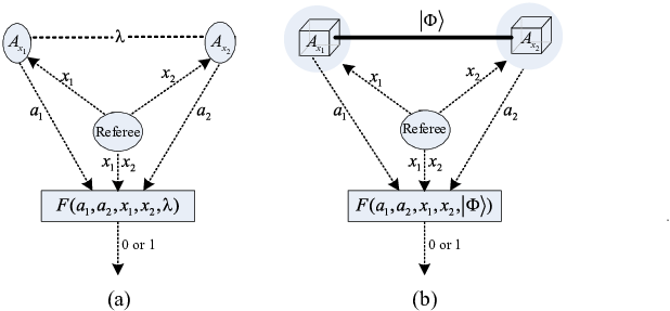
Refer to caption
Figure 6: (Color online) The Bell test derived from the inequality (E1). Here, some functional box FF (depending fif_{i} in Eqs.(E2) and (E3)) that depends on the shared sources will be used. (a) The classical hidden variable model. Two parties share one hidden variable λ\lambda or a bipartite separable state ρ=∑ipi​ρi(1)⊗ρi(2)\rho=\sum_{i}p_{i}\rho^{(1)}_{i}\otimes\rho^{(2)}_{i}, where {pi}\{p_{i}\} is a probability distribution and ρi(j)\rho^{(j)}_{i}s are density operators of the jj-th system, j=1,2j=1,2. (b) The quantum entangled system. Two parties share one entangled pure state |Φ⟩|\Phi\rangle. The measurement operator AxiA_{x_{i}} depends on the input xix_{i}, i=1,2i=1,2. In what follows, we denote Figure x in Supplementary file as Figure Sx for convenience, which is used to distinguish these from the main text.

Proof of Inequality (E1). Note that −fi​(ρ,X)-f_{i}(\rho,X) is convex functional for ρ\rho Lieb, i.e.,

−f1​(λ​ρ1+(1−λ)​ρ2,A)≤−λ​f1​(ρ1,A)−(1−λ)​f1​(ρ2,A)\displaystyle-f_{1}(\lambda\rho_{1}+(1-\lambda)\rho_{2},A)\leq-\lambda{}f_{1}(\rho_{1},A)-(1-\lambda)f_{1}(\rho_{2},A)
−f2​(λ​ρ1+(1−λ)​ρ2,A,B)≤−λ​f2​(ρ1,A,B)−(1−λ)​f2​(ρ2,A,B)\displaystyle-f_{2}(\lambda\rho_{1}+(1-\lambda)\rho_{2},A,B)\leq-\lambda{}f_{2}(\rho_{1},A,B)-(1-\lambda)f_{2}(\rho_{2},A,B) (E4)

where ρ1\rho_{1} and ρ2\rho_{2} are density operators, and AA and BB are measurement operators. For a given measurement operator AA, it follows that

maxρ=∑ipi​ϱi(1)⊗ϱi(2)⁡{−f1​(ρ,A)}=\displaystyle\max_{\rho=\sum_{i}p_{i}\varrho^{(1)}_{i}\otimes\varrho^{(2)}_{i}}\{-f_{1}(\rho,A)\}= maxρ=ϱ(1)⊗ϱ(2)⁡{−f1​(ρ,A)}\displaystyle\max_{\rho=\varrho^{(1)}\otimes\varrho^{(2)}}\{-f_{1}(\rho,A)\}
=\displaystyle= maxρ=|ψ1⟩​⟨ψ1|⊗|ψ2⟩​⟨ψ2|⁡{−f1​(ρ,A)}\displaystyle\max_{\rho=|\psi_{1}\rangle\langle\psi_{1}|\otimes|\psi_{2}\rangle\langle\psi_{2}|}\{-f_{1}(\rho,A)\} (E5)

where ϱ(i)\varrho^{(i)} can be represented by linearly superposition of pure states, i.e., ϱ(i)=∑jqj(i)​|ψj(i)⟩​⟨ψj(i)|\varrho^{(i)}=\sum_{j}q^{(i)}_{j}|\psi^{(i)}_{j}\rangle\langle\psi^{(i)}_{j}|, and {qj(i)}\{q^{(i)}_{j}\} is a probability distribution. Similar result holds for −f2​(ρ,A,B)-f_{2}(\rho,A,B). For a product state |ψ1⟩​|ψ2⟩|\psi_{1}\rangle|\psi_{2}\rangle, and two local measurement operators AA and BB, it is easy to check that

f1​(|ψ1⟩​|ψ2⟩,A)=⟨ψ1|A|ψ1⟩2,\displaystyle f_{1}(|\psi_{1}\rangle|\psi_{2}\rangle,A)=\langle\psi_{1}|A|\psi_{1}\rangle^{2},
f1​(|ψ1⟩​|ψ2⟩,B)=⟨ψ2|B|ψ2⟩2,\displaystyle f_{1}(|\psi_{1}\rangle|\psi_{2}\rangle,B)=\langle\psi_{2}|B|\psi_{2}\rangle^{2},
f2​(|ψ1⟩​|ψ2⟩,A,B)=⟨ψ1|A|ψ1⟩​⟨ψ2|B|ψ2⟩.\displaystyle f_{2}(|\psi_{1}\rangle|\psi_{2}\rangle,A,B)=\langle\psi_{1}|A|\psi_{1}\rangle\langle\psi_{2}|B|\psi_{2}\rangle. (E6)

From Eqs.(E5) and (E6), the left side of Eq.(E1) is given

ω:=\displaystyle\omega:= maxρ=∑ipi​ϱi(1)⊗ϱi(2)⁡{2​⟨A⊗B⟩ρ−12​f1​(ρ,A)−12​f1​(ρ,B)−f2​(ρ,A,B)}\displaystyle\max_{\rho=\sum_{i}p_{i}\varrho^{(1)}_{i}\otimes\varrho^{(2)}_{i}}\{2\langle{}A\otimes{}B\rangle_{\rho}-\frac{1}{2}f_{1}(\rho,A)-\frac{1}{2}f_{1}(\rho,B)-f_{2}(\rho,A,B)\}
≤\displaystyle\leq maxρ=|ψ1⟩​⟨ψ1|​|ψ2⟩​⟨ψ2|⁡{2​⟨A⊗B⟩ρ−12​f1​(ρ,A)−12​f1​(ρ,B)−f2​(ρ,A,B)}\displaystyle\max_{\rho=|\psi_{1}\rangle\langle\psi_{1}||\psi_{2}\rangle\langle\psi_{2}|}\{2\langle{}A\otimes{}B\rangle_{\rho}-\frac{1}{2}f_{1}(\rho,A)-\frac{1}{2}f_{1}(\rho,B)-f_{2}(\rho,A,B)\} (E7)
=\displaystyle= maxρ=|ψ1⟩​⟨ψ1|​|ψ2⟩​⟨ψ2|{⟨A⟩⟨B⟩|ψ2⟩|ψ1⟩−12⟨A⟩|ψ1⟩2−12⟨B⟩|ψ2⟩2}\displaystyle\max_{\rho=|\psi_{1}\rangle\langle\psi_{1}||\psi_{2}\rangle\langle\psi_{2}|}\{\langle{}A\rangle{}_{|\psi_{1}\rangle}\langle{}B\rangle_{|\psi_{2}\rangle}-\frac{1}{2}\langle{}A\rangle_{|\psi_{1}\rangle}^{2}-\frac{1}{2}\langle{}B\rangle^{2}_{|\psi_{2}\rangle}\} (E8)
≤\displaystyle\leq 0\displaystyle 0 (E9)

which implies the inequality (E1). Eq.(E7) follows from Eq.(E5) and the linearity of the expectation operation ⟨⋅⟩\langle{}\cdot{}\rangle. Inequality (E8) follows from Eq.(E6). Inequality (E9) follows from the inequality: (x+y)2≥0(x+y)^{2}\geq 0.

Note that −f1-f_{1} and −f2-f_{2} are convex in the density operator ρ\rho Lieb. It only needs to consider pure states for the maximum. The left side of Eq.(E1) is given by

ωq:=\displaystyle\omega_{q}:= maxρ=∑ipi​|Ψi⟩​⟨Ψi|⁡{2​⟨A⊗B⟩ρ−12​f1​(ρ,A,B)−12​f1​(ρ,A,B)−f2​(ρ,A,B)}\displaystyle\max_{\rho=\sum_{i}p_{i}|\Psi_{i}\rangle\langle\Psi_{i}|}\{2\langle{}A\otimes{}B\rangle_{\rho}-\frac{1}{2}f_{1}(\rho,A,B)-\frac{1}{2}f_{1}(\rho,A,B)-f_{2}(\rho,A,B)\}
≤\displaystyle\leq max|Ψ⟩⁡{⟨(A⊗𝟙+𝟙⊗B)2⟩|Ψ⟩−12​f1​(|Ψ⟩,A)−12​f1​(|Ψ⟩,B)−f2​(|Ψ⟩,A,B)}−2\displaystyle\max_{|\Psi\rangle}\{\langle(A\otimes{}\mathbbm{1}+\mathbbm{1}\otimes{}B)^{2}\rangle_{|\Psi\rangle}-\frac{1}{2}f_{1}(|\Psi\rangle,A)-\frac{1}{2}f_{1}(|\Psi\rangle,B)-f_{2}(|\Psi\rangle,A,B)\}-2 (E10)
=\displaystyle= max|Ψ⟩⁡(⟨(A⊗𝟙+𝟙⊗B)2⟩|Ψ⟩−12​⟨A⊗𝟙+𝟙⊗B⟩|Ψ⟩2)−2\displaystyle\max_{|\Psi\rangle}(\langle(A\otimes{}\mathbbm{1}+\mathbbm{1}\otimes{}B)^{2}\rangle_{|\Psi\rangle}-\frac{1}{2}\langle{}A\otimes{}\mathbbm{1}+\mathbbm{1}\otimes{}B\rangle_{|\Psi\rangle}^{2})-2 (E11)
≤\displaystyle\leq 2\displaystyle 2 (E12)

Eq.(E10) follows from the assumptions of A,B≤𝟙A,B\leq\mathbbm{1}. Eq.(E11) follows from the equality: f1​(|Ψ⟩,A)=⟨A⊗𝟙⟩|Ψ⟩2f_{1}(|\Psi\rangle,A)=\langle A\otimes\mathbbm{1}\rangle_{|\Psi\rangle}^{2}, f1​(|Ψ⟩,B)=⟨𝟙⊗B⟩|Ψ⟩2f_{1}(|\Psi\rangle,B)=\langle\mathbbm{1}\otimes B\rangle_{|\Psi\rangle}^{2}, and f2​(|Ψ⟩,A,B)=⟨A⊗B⟩|Ψ⟩f_{2}(|\Psi\rangle,A,B)=\langle A\otimes B\rangle_{|\Psi\rangle}. Inequality (E12) makes use of the inequalities: ⟨(A⊗𝟙+𝟙⊗B)2⟩≤4\langle(A\otimes{}\mathbbm{1}+\mathbbm{1}\otimes{}B)^{2}\rangle\leq 4 and ⟨A⊗𝟙+𝟙⊗B⟩2≥0\langle A\otimes{}\mathbbm{1}+\mathbbm{1}\otimes{}B\rangle^{2}\geq 0. □\square

Example S1. Consider a bipartite entangled pure state |Ψ⟩|\Psi\rangle as

|Ψ⟩=cos⁡θ⁡|00⟩+sin⁡θ⁡|11⟩\displaystyle|\Psi\rangle=\cos\theta|00\rangle+\sin\theta|11\rangle (E13)

where θ∈(0,π2]\theta\in(0,\frac{\pi}{2}]. Define A=B=σxA=B=\sigma_{x} as Pauli operator. It is easy to evaluate that

ωq=\displaystyle\omega_{q}= 2⟨A⊗B⟩|Ψ⟩−12f1(|Ψ⟩,A)−12f1(|Ψ⟩,B)−12f2(|Ψ⟩,A,B)]\displaystyle 2\langle{}A\otimes{}B\rangle_{|\Psi\rangle}-\frac{1}{2}f_{1}(|\Psi\rangle,A)-\frac{1}{2}f_{1}(|\Psi\rangle,B)-\frac{1}{2}f_{2}(|\Psi\rangle,A,B)]
=\displaystyle= 2​t​r​[(A⊗B)​|Ψ⟩​⟨Ψ|]−12​(tr​[(A⊗𝟙)​|Ψ⟩​⟨Ψ|]2+tr⁡[(𝟙⊗B)​|Ψ⟩​⟨Ψ|])2\displaystyle 2{\rm tr}[(A\otimes{}B)|\Psi\rangle\langle\Psi|]-\frac{1}{2}({\rm tr}[(A\otimes{}\mathbbm{1})|\Psi\rangle\langle\Psi|]^{2}+{\rm tr}[(\mathbbm{1}\otimes{}B)|\Psi\rangle\langle\Psi|])^{2}
=\displaystyle= 4​sin⁡2​θ\displaystyle 4\sin 2\theta
>\displaystyle> 0\displaystyle 0 (E14)

when θ∈(0,π2]\theta\in(0,\frac{\pi}{2}], where tr⁡[(A⊗𝟙)​|Ψ⟩​⟨Ψ|]=tr⁡[(𝟙⊗B)​|Ψ⟩​⟨Ψ|]=0{\rm tr}[(A\otimes{}\mathbbm{1})|\Psi\rangle\langle\Psi|]={\rm tr}[(\mathbbm{1}\otimes{}B)|\Psi\rangle\langle\Psi|]=0. If define A=B=σzA=B=\sigma_{z}, we get ωq=2−2​cos⁡2​θ2>0\omega_{q}=2-2\cos 2\theta^{2}>0 for θ∈(0,π2)\theta\in(0,\frac{\pi}{2}), where tr⁡[(A⊗𝟙)​|Ψ⟩​⟨Ψ|]=tr⁡[(𝟙⊗B)​|Ψ⟩​⟨Ψ|]=cos⁡2​θ{\rm tr}[(A\otimes{}\mathbbm{1})|\Psi\rangle\langle\Psi|]={\rm tr}[(\mathbbm{1}\otimes{}B)|\Psi\rangle\langle\Psi|]=\cos 2\theta. Hence, two pauli measurement operators are useful to verify generalized bipartite entangled pure states. Interestingly, the maximally entangled |Ψ⟩|\Psi\rangle achieves the maximal violation.

Similarly, consider a generalized bipartite entangled pure state on Hilbert space ℍA⊗ℍB\mathbb{H}_{A}\otimes\mathbb{H}_{B} as

|Ψ⟩=∑i=0d−1ai​|i​i⟩\displaystyle|\Psi\rangle=\sum_{i=0}^{d-1}a_{i}|ii\rangle (E15)

where ℍA\mathbb{H}_{A} and ℍB\mathbb{H}_{B} have the same dimension d≥2d\geq 2, and γi\gamma_{i} satisfies ∑i=0d−1ai2=1\sum_{i=0}^{d-1}a_{i}^{2}=1. It is entangled if ai​aj≠0a_{i}a_{j}\not=0 for some i≠ji\not=j. Consider the subspace spanned by {|i⟩,|j⟩}\{|i\rangle,|j\rangle\}. It is easy to prove that Pauli operators σx,σz\sigma_{x},\sigma_{z} on the subspace can also be used to verify the nonlocality of |Ψ⟩|\Psi\rangle.

E2. Multipartite entangled states

Consider an nn-partite state ρ\rho on Hilbert space ℍA1⊗⋯⊗ℍAn\mathbb{H}_{A_{1}}\otimes\cdots\otimes\mathbb{H}_{A_{n}} with the same dimension d≥2d\geq 2. ρ\rho is fully separable Sy if the following decomposition holds

ρ=∑ipiρ(1)i⊗⋯⊗ρ(n)i\displaystyle\rho=\sum_{i}p_{i}\rho^{(1)}_{i}\otimes\cdots{}\otimes\rho^{(n)}_{i} (E16)

where {pi}\{p_{i}\} is a probability distribution, and ρi(j)\rho^{(j)}_{i}s are density operators on the local system of AjA_{j}, j=1,⋯,nj=1,\cdots,n. Inequality (E1) can be then extended as:

∑1≤i≠j≤n⟨Mi⊗Mj⟩ρ−n−1n​∑i=1n(f1​(ρ,Mi)+∑j≠inf2​(ρ,Mi,Mj))≤0\displaystyle\sum_{1\leq i\not=j\leq n}\langle{}M_{i}\otimes{}M_{j}\rangle_{\rho}-\frac{n-1}{n}\sum_{i=1}^{n}(f_{1}(\rho,M_{i})+\sum_{j\not=i}^{n}f_{2}(\rho,M_{i},M_{j}))\leq 0 (E17)

for any fully separable state ρ\rho, where f1f_{1} and f2f_{2} are two nonlinear functionals defined in the respective Eqs.(E2) and (E3), and MiM_{i}s are dichotomic measurement operators. On the other hand, the maximum of l.h.s of Eq.(E17) is n2−nn^{2}-n for general quantum states. This inequality can be used to verify multipartite entangled states.

Proof of Inequality (E17). Similar to bipartite states, −fi-f_{i}s are convex for the density operators with any measurement operators MiM_{i} Lieb. Consider any fully separable pure state of ρf​s=⊗i=1n|ψi⟩⟨ψi|\rho_{fs}=\otimes_{i=1}^{n}|\psi_{i}\rangle\langle\psi_{i}|. The left side of the inequality (E17) is rewritten by:

ω:=\displaystyle\omega:= maxρf​s⁡{∑1≤i≠j≤n⟨Mi⊗Mj⟩ρ−n−1n​∑i=1n(f1​(ρ,Mi)+∑j≠if2​(ρ,Mi,Mj))}\displaystyle\max_{\rho_{fs}}\{\sum_{1\leq i\not=j\leq n}\langle{}M_{i}\otimes{}M_{j}\rangle_{\rho}-\frac{n-1}{n}\sum_{i=1}^{n}(f_{1}(\rho,M_{i})+\sum_{j\not=i}f_{2}(\rho,M_{i},M_{j}))\}
≤\displaystyle\leq maxρ=⊗i=1n|ψi⟩{∑1≤i≠j≤n⟨Mi⊗Mj⟩ρ−n−1n∑i=1n(f1(ρ,Mi)+∑j≠if2(ρ,Mi,Mj))}\displaystyle\max_{\rho=\otimes_{i=1}^{n}|\psi_{i}\rangle}\{\sum_{1\leq i\not=j\leq n}\langle{}M_{i}\otimes{}M_{j}\rangle_{\rho}-\frac{n-1}{n}\sum_{i=1}^{n}(f_{1}(\rho,M_{i})+\sum_{j\not=i}f_{2}(\rho,M_{i},M_{j}))\} (E18)
≤\displaystyle\leq maxρ=⊗i=1n|ψi⟩{⟨(∑j=1nMi)2⟩ρ−n2−n−1n∑i=1n(f1(ρ,Mi)−∑j≠if2(ρ,Mi,Mj))}\displaystyle\max_{\rho=\otimes_{i=1}^{n}|\psi_{i}\rangle}\{\langle(\sum_{j=1}^{n}M_{i})^{2}\rangle_{\rho}-n^{2}-\frac{n-1}{n}\sum_{i=1}^{n}(f_{1}(\rho,M_{i})-\sum_{j\not=i}f_{2}(\rho,M_{i},M_{j}))\} (E19)
=\displaystyle= max⊗i=1n|ψi⟩{1n∑1≤i≠j≤n⟨Mi⟩|ψi⟩⟨Mj⟩|ψj⟩−n−1n∑i=1n⟨Mi⟩|ψi⟩2}−n\displaystyle\max_{\otimes_{i=1}^{n}|\psi_{i}\rangle}\{\frac{1}{n}\sum_{1\leq i\not=j\leq n}\langle{}M_{i}\rangle_{|\psi_{i}\rangle}\langle{}M_{j}\rangle_{|\psi_{j}\rangle}-\frac{n-1}{n}\sum_{i=1}^{n}\langle{}M_{i}\rangle_{|\psi_{i}\rangle}^{2}\}-n (E20)
≤\displaystyle\leq 0\displaystyle 0 (E21)

Inequality (E18) follows from the convexity of −fi-f_{i}s. Inequality (E19) follows from Mi≤𝟙M_{i}\leq\mathbbm{1}. Eq.(E20) follows from the equalities: f1(⊗i=1n|ψi⟩,Mj)=(⟨ψi|⊗i=1n)Mj(⊗k=1n|ψk⟩):=⟨Mj⟩|ψj⟩f_{1}(\otimes_{i=1}^{n}|\psi_{i}\rangle,M_{j})=(\langle{}\psi_{i}|\otimes_{i=1}^{n})M_{j}(\otimes_{k=1}^{n}|\psi_{k}\rangle):=\langle{}M_{j}\rangle_{|\psi_{j}\rangle}. Inequality (E21) follows from the inequality: ∑1≤i≠j≤n⟨Mi⟩|ψi⟩​⟨Mj⟩|ψj⟩−(n−1)​∑i=1n⟨Mi⟩|ψi⟩2=∑1≤i<j≤n(⟨Mi⟩|ψi⟩+⟨Mj⟩|ψj⟩)2≥0\sum_{1\leq i\not=j\leq n}\langle{}M_{i}\rangle_{|\psi_{i}\rangle}\langle{}M_{j}\rangle_{|\psi_{j}\rangle}-(n-1)\sum_{i=1}^{n}\langle{}M_{i}\rangle_{|\psi_{i}\rangle}^{2}=\sum_{1\leq i<j\leq n}(\langle{}M_{i}\rangle_{|\psi_{i}\rangle}+\langle{}M_{j}\rangle_{|\psi_{j}\rangle})^{2}\geq 0.

For an nn-partite quantum state of ρ=∑ipi​|Φi⟩​⟨Φi|\rho=\sum_{i}p_{i}|\Phi_{i}\rangle\langle\Phi_{i}|, with similar evaluation, the left side of Eq.(E17) is rewritten by:

ωq:=\displaystyle\omega_{q}:= maxρ⁡{∑1≤i≠j≤n⟨Mi⊗Mj⟩ρ−n−1n​∑i=1n(f1​(ρ,Mi)+∑j≠if2​(ρ,Mi,Mj))}\displaystyle\max_{\rho}\{\sum_{1\leq i\not=j\leq n}\langle{}M_{i}\otimes{}M_{j}\rangle_{\rho}-\frac{n-1}{n}\sum_{i=1}^{n}(f_{1}(\rho,M_{i})+\sum_{j\not=i}f_{2}(\rho,M_{i},M_{j}))\}
≤\displaystyle\leq maxρ=|Φ⟩​⟨Φ|⁡{∑1≤i≠j≤n⟨Mi⊗Mj⟩ρ−n−1n​∑i=1n(f1​(ρ,Mi)+∑j≠if2​(ρ,Mi,Mj))}\displaystyle\max_{\rho=|\Phi\rangle\langle\Phi|}\{\sum_{1\leq i\not=j\leq n}\langle{}M_{i}\otimes{}M_{j}\rangle_{\rho}-\frac{n-1}{n}\sum_{i=1}^{n}(f_{1}(\rho,M_{i})+\sum_{j\not=i}f_{2}(\rho,M_{i},M_{j}))\} (E22)
≤\displaystyle\leq max|Φ⟩⁡{⟨(∑i=1nMi)2⟩|Φ⟩−n−1n​∑i=1n(f1​(|Φ⟩,Mi)+∑j≠if2​(|Φ⟩,Mi,Mj))}−n\displaystyle\max_{|\Phi\rangle}\{\langle{}(\sum_{i=1}^{n}M_{i})^{2}\rangle_{|\Phi\rangle}-\frac{n-1}{n}\sum_{i=1}^{n}(f_{1}(|\Phi\rangle,M_{i})+\sum_{j\not=i}f_{2}(|\Phi\rangle,M_{i},M_{j}))\}-n (E23)
=\displaystyle= max|Φ⟩⁡{⟨(∑i=1nMi)2⟩|Φ⟩−n−1n​(∑i=1n⟨Mi⟩|Φ⟩)2}−n\displaystyle\max_{|\Phi\rangle}\{\langle{}(\sum_{i=1}^{n}M_{i})^{2}\rangle_{|\Phi\rangle}-\frac{n-1}{n}(\sum_{i=1}^{n}\langle M_{i}\rangle_{|\Phi\rangle})^{2}\}-n (E24)
≤\displaystyle\leq n2−n\displaystyle n^{2}-n (E25)

Inequality (E22) follows from the convexity of −fi-f_{i}s. Inequality (E23) follows from the assumptions of Mi≤𝟙M_{i}\leq\mathbbm{1} for all MiM_{i}s. Eq.(E23) follows from the equalities: f1​(|Φ⟩,Mj)=⟨Φ|Mj|Φ⟩:=⟨Mj⟩f_{1}(|\Phi\rangle,M_{j})=\langle{}\Phi|M_{j}|\Phi\rangle:=\langle{}M_{j}\rangle. Inequality (A24) follows from the inequalities: ⟨(∑i=1nMi)2⟩≤n2\langle{}(\sum_{i=1}^{n}M_{i})^{2}\rangle\leq n^{2} and (∑i=1n⟨Mi⟩|Φ⟩)2≥0(\sum_{i=1}^{n}\langle M_{i}\rangle_{|\Phi\rangle})^{2}\geq 0. □\square

In what follows, some examples will be presented to show the maximal violation of the inequality (E17).

Example S2. Consider an nn-partite generalized GHZ state GHZ:

|Φ⟩=cos⁡θ​|0⟩⊗n+sin⁡θ​|1⟩⊗n\displaystyle|\Phi\rangle=\cos\theta|0\rangle^{\otimes n}+\sin\theta|1\rangle^{\otimes n} (E26)

with θ∈(0,π4]\theta\in(0,\frac{\pi}{4}]. Define Mi=σzM_{i}=\sigma_{z}, i=1,⋯,ni=1,\cdots,n. It follows that

ωq​(|Φ⟩)=\displaystyle\omega_{q}(|\Phi\rangle)= n2−n−n⁡(n−1)​cos⁡2​θ2>0\displaystyle n^{2}-n-n(n-1)\cos 2\theta^{2}>0 (E27)

for any θ∈(0,π4]\theta\in(0,\frac{\pi}{4}]. It means that generalized GHZ states are not fully separable for any θ∈(0,π4]\theta\in(0,\frac{\pi}{4}].

Example S3. Consider an nn-partite generalized W state

|W⟩=∑i=1nαi​|0⟩⊗i−1​|1⟩​|0⟩⊗n−i\displaystyle|W\rangle=\sum_{i=1}^{n}\alpha_{i}|0\rangle^{\otimes i-1}|1\rangle|0\rangle^{\otimes n-i}

with ∑i=1nαi2=1\sum_{i=1}^{n}\alpha_{i}^{2}=1 and αi≥0\alpha_{i}\geq 0. Define Mi=σxM_{i}=\sigma_{x}, i=1,⋯,ni=1,\cdots,n. It follows that

ωq​(|W⟩)=\displaystyle\omega_{q}(|W\rangle)= ∑1≤i≠j≤n4​αi​αj\displaystyle\sum_{1\leq i\not=j\leq n}4\alpha_{i}\alpha_{j}
>\displaystyle> 0\displaystyle 0 (E28)

for αi​αj≠0\alpha_{i}\alpha_{j}\not=0 with any i≠ji\not=j, which implies a generalized singlet state for subsystems i,ji,j.

Example S4. Consider a generalized 44-partite Dicke state Dicke1:

|D2,4⟩=\displaystyle|D_{2,4}\rangle= γ1​|0011⟩+γ2​|1100⟩+γ3​|0101⟩+γ4​|1010⟩+γ5​|1001⟩+γ6​|0110⟩\displaystyle\gamma_{1}|0011\rangle+\gamma_{2}|1100\rangle+\gamma_{3}|0101\rangle+\gamma_{4}|1010\rangle+\gamma_{5}|1001\rangle+\gamma_{6}|0110\rangle (S29)

where γi\gamma_{i}s satisfy ∑i=16γi2=1\sum_{i=1}^{6}\gamma_{i}^{2}=1. Define Mi=σx,i=1,⋯,nM_{i}=\sigma_{x},i=1,\cdots,n. It follows that

ωq​(|D2,4⟩)=\displaystyle\omega_{q}(|D_{2,4}\rangle)= ∑1≤i<j≤68​γi​γj>0\displaystyle\sum_{1\leq i<j\leq 6}8\gamma_{i}\gamma_{j}>0 (S30)

for all nonnegative γi\gamma_{i} with at least two γi,γj≠0\gamma_{i},\gamma_{j}\not=0.

Now, we consider genuinely multipartite entangled states in the biseparable model. For a general nn-partite state ρ\rho on Hilbert space ℍA1⊗⋯⊗ℍAn\mathbb{H}_{A_{1}}\otimes{}\cdots{}\otimes\mathbb{H}_{A_{n}}, it is kk-producible state Sy if the following decomposition holds

ρk​-pr=∑I1,⋯,Ik∑ipiρ(I1)i⊗⋯⊗ρ(Ik)i\displaystyle\rho_{k\mbox{\small-pr}}=\sum_{I_{1},\cdots,I_{k}}\sum_{i}p_{i}\rho^{(I_{1})}_{i}\otimes{}\cdots\otimes\rho^{(I_{k})}_{i} (E31)

where {I1,⋯,Ik}\{I_{1},\cdots,I_{k}\} is a kk-partite partition of {1,⋯,n}\{1,\cdots,n\}, i.e., ∪i=1kIi={1,⋯,n}\cup_{i=1}^{k}I_{i}=\{1,\cdots,n\} and Ii∩Ij=∅I_{i}\cap{}I_{j}=\emptyset for i≠ji\not=j, ρi(Ij)\rho^{(I_{j})}_{i} are density operators of local system IjI_{j}. We can prove the following inequality

∑1≤i≠j≤n1n​⟨Mi⊗Mj⟩ρ−n−1n2​∑i=1n(f1​(ρ,Mi)+∑j≠inf2​(ρ,Mi,Mj))≤k−1\displaystyle\sum_{1\leq i\not=j\leq n}\frac{1}{n}\langle{}M_{i}\otimes{}M_{j}\rangle_{\rho}-\frac{n-1}{n^{2}}\sum_{i=1}^{n}(f_{1}(\rho,M_{i})+\sum_{j\not=i}^{n}f_{2}(\rho,M_{i},M_{j}))\leq k-1 (E32)

for all kk-producible nn-partite states ρ\rho. The upper bound is n−1n-1 for any biseparable states Sy.

Proof of Inequality (E32). Actually, the left side of Eq.(E32) is rewritten by:

ωk:=\displaystyle\omega_{k}:= maxρk​-pr∑1≤i≠j≤n1n⟨Mi⊗Mj⟩ρk​-pr−n−1n2∑i=1n(f1(ρρk​-pr,Mi)+∑j≠if2(ρρk​-pr,Mi,Mj))}\displaystyle\max_{\rho_{k\mbox{\small-pr}}}\sum_{1\leq i\not=j\leq n}\frac{1}{n}\langle{}M_{i}\otimes{}M_{j}\rangle_{\rho_{k\mbox{\small-pr}}}-\frac{n-1}{n^{2}}\sum_{i=1}^{n}(f_{1}(\rho_{\rho_{k\mbox{\small-pr}}},M_{i})+\sum_{j\not=i}f_{2}(\rho_{\rho_{k\mbox{\small-pr}}},M_{i},M_{j}))\}
≤\displaystyle\leq maxρ=⊗i=1m|Φi⟩Ii⟨Φi|{∑1≤i≠j≤n1n⟨Mi⊗Mj⟩ρ−n−1n2∑i=1n(f1(ρ,Mi)+∑j≠if2(ρ,Mi,Mj))}\displaystyle\max_{\rho=\otimes_{i=1}^{m}|\Phi_{i}\rangle_{I_{i}}\langle\Phi_{i}|}\{\sum_{1\leq i\not=j\leq n}\frac{1}{n}\langle{}M_{i}\otimes{}M_{j}\rangle_{\rho}-\frac{n-1}{n^{2}}\sum_{i=1}^{n}(f_{1}(\rho,M_{i})+\sum_{j\not=i}f_{2}(\rho,M_{i},M_{j}))\} (E33)
≤\displaystyle\leq maxρ=⊗i=1m|Φi⟩Ii⟨Φi|{1n⟨(∑i=1nMi)2⟩ρ−n−1n2∑i=1n(f1(ρ,Mi)+∑j≠if2(ρ,Mi,Mj))}−1\displaystyle\max_{\rho=\otimes_{i=1}^{m}|\Phi_{i}\rangle_{I_{i}}\langle\Phi_{i}|}\{\frac{1}{n}\langle{}(\sum_{i=1}^{n}M_{i})^{2}\rangle_{\rho}-\frac{n-1}{n^{2}}\sum_{i=1}^{n}(f_{1}(\rho,M_{i})+\sum_{j\not=i}f_{2}(\rho,M_{i},M_{j}))\}-1 (E34)
=\displaystyle= 1n2maxρ=⊗i=1m|Φi⟩Ii⟨Φi|{⟨(∑i=1nMi)2⟩ρ+(n−1)I(ρ,∑i=1nMi)}−1\displaystyle\frac{1}{n^{2}}\max_{\rho=\otimes_{i=1}^{m}|\Phi_{i}\rangle_{I_{i}}\langle\Phi_{i}|}\{\langle{}(\sum_{i=1}^{n}M_{i})^{2}\rangle_{\rho}+(n-1)I(\rho,\sum_{i=1}^{n}M_{i})\}-1 (E35)
≤\displaystyle\leq 1n2​(n​k+(n−1)​max⁡∑i=1mn1+⋯+nm=n,1≤n1,⋯,nm≤k⁡ni2)−1\displaystyle\frac{1}{n^{2}}(nk+(n-1)\max_{n_{1}+\cdots+n_{m}=n,\atop{1\leq n_{1},\cdots,n_{m}\leq k}}\sum_{i=1}^{m}n_{i}^{2})-1 (E36)
≤\displaystyle\leq 1n×k2×nk−1\displaystyle\frac{1}{n}\times{}k^{2}\times\frac{n}{k}-1 (E37)
=\displaystyle= k−1\displaystyle k-1 (E38)

Inequality (E33) follows from the convexity of −fi-f_{i}s Lieb. Inequality (E34) follows from the assumptions of Mi≤𝟙M_{i}\leq\mathbbm{1} for all iis. Eq.(E35) follows from the definition of Wigner-Yanase skew information II WY. Note that I⁡(|ϕi⟩​|ϕj⟩,Mi+Mj)=I⁡(|ϕi⟩,Mi)+I⁡(|ϕj⟩,Mj)I(|\phi_{i}\rangle|\phi_{j}\rangle,M_{i}+M_{j})=I(|\phi_{i}\rangle,M_{i})+I(|\phi_{j}\rangle,M_{j}) holds for any product states. From the inequality of maxρ=⊗i=1m|Φi⟩Ii⟨Φi|⟨(∑i=1nMi)2⟩ρ<maxρ=⊗i=1m|Ψi⟩Ii⟨Φi|(n−1)I(ρ,∑i=1nMi)\max_{\rho=\otimes_{i=1}^{m}|\Phi_{i}\rangle_{I_{i}}\langle\Phi_{i}|}\langle{}(\sum_{i=1}^{n}M_{i})^{2}\rangle_{\rho}<\max_{\rho=\otimes_{i=1}^{m}|\Psi_{i}\rangle_{I_{i}}\langle\Phi_{i}|}(n-1)I(\rho,\sum_{i=1}^{n}M_{i}), it follows that maxρ=⊗i=1m|Φi⟩Ii⟨Φi|(⟨(∑i=1nMi)2⟩ρ+(n−1)I(ρ,∑i=1nMi))\max_{\rho=\otimes_{i=1}^{m}|\Phi_{i}\rangle_{I_{i}}\langle\Phi_{i}|}(\langle(\sum_{i=1}^{n}M_{i})^{2}\rangle_{\rho}+(n-1)I(\rho,\sum_{i=1}^{n}M_{i})) given in the right side of Eq.(E36) is achieved for ρ=⊗i=1m|Φi⟩Ii⟨Φi|\rho=\otimes_{i=1}^{m}|\Phi_{i}\rangle_{I_{i}}\langle\Phi_{i}|, which maximizes (n−1)​I​(ρ,∑i=1nMi)(n-1)I(\rho,\sum_{i=1}^{n}M_{i}). In this case, ⟨(∑i=1nMi)2⟩ρ=∑j=1m⟨(∑IjMs)2⟩ρ≤k2×nk=n​k\langle(\sum_{i=1}^{n}M_{i})^{2}\rangle_{\rho}=\sum_{j=1}^{m}\langle{}(\sum_{I_{j}}M_{s})^{2}\rangle_{\rho}\leq k^{2}\times\frac{n}{k}=nk. This has proved the inequality (E37). Inequality (E38) has taken use of the following inequality: ∑i=1mni2≤(m−1)​k2+nm2≤k2×nk\sum_{i=1}^{m}n_{i}^{2}\leq(m-1)k^{2}+n_{m}^{2}\leq k^{2}\times\frac{n}{k}, where n1=n2=⋯=nm−1=kn_{1}=n_{2}=\cdots=n_{m-1}=k.

The maximum of the quantity in the left side of Eq.(E32) is n−1n-1 for nn-partite genuinely entangled state in the biseparable model Sy. □\square

This witness is device-independent in the sense that any observed violation of ωk−p​r\omega_{k-pr} by ρ\rho implies that ρ\rho is at least genuinely k+1k+1-partite entangled, i.e., it has an entanglement depth of at least k+1k+1 in the biseparable model Sy, regardless of the details of measurement devices and Hilbert space dimensions.

Example S5. Consider an nn-partite generalized GHZ states |Φ⟩=cos⁡θ​|0⟩⊗n+sin⁡θ​|1⟩⊗n|\Phi\rangle=\cos\theta|0\rangle^{\otimes n}+\sin\theta|1\rangle^{\otimes n} with θ∈(0,π2]\theta\in(0,\frac{\pi}{2}]. Define Mi=σzM_{i}=\sigma_{z}, γi=1\gamma_{i}=1 for all iis. It follows that

ωk​-pr​(|Φ⟩)=\displaystyle\omega_{k\mbox{\small-pr}}(|\Phi\rangle)= n−1−(n−1)​cos⁡2​θ2\displaystyle n-1-(n-1)\cos 2\theta^{2}
>\displaystyle> k−1\displaystyle k-1 (E39)

when cos⁡2​θ<n−kn−1\cos 2\theta<\sqrt{\frac{n-k}{n-1}}. It implies that the inequality (E32) can be used to verify the entanglement depth k≥2k\geq 2 for the maximally GHZ state or partially entangled GHZ states. Some numerical simulations of θ\theta are shown in Figure S7. Specially, when k=n−1k=n-1, it shows that the inequality (E32) can be used to verify the genuinely multipartite nonlocality of partially entangled GHZ states with cos⁡2​θ<n−2n−1\cos 2\theta<\sqrt{\frac{n-2}{n-1}} in the biseparable model Sy. From Theorem 2, it means that the inequality (E32) can be used to verify new genuinely multipartite nonlocality of partially entangled GHZ states with cos⁡2​θ<n−2n−1\cos 2\theta<\sqrt{\frac{n-2}{n-1}} in the present model.

Refer to caption
Figure 7: (Color online) The lower bound of θ\theta for verifying the entanglement depth of generalized GHZ states in terms of the number nn of particles in the biseparable model Sy.

Example S6. Consider an nn-partite W state |Wn⟩=∑i=1nγi​|0⟩⊗i−1​|1⟩​|0⟩⊗n−i|W_{n}\rangle=\sum_{i=1}^{n}\gamma_{i}|0\rangle^{\otimes i-1}|1\rangle|0\rangle^{\otimes n-i} with ∑iγi2=1\sum_{i}\gamma_{i}^{2}=1. Define Ai=σxA_{i}=\sigma_{x} for all iis. It follows that

ωk​-pr​(|Wn⟩)=\displaystyle\omega_{k\mbox{\small-pr}}(|W_{n}\rangle)= ∑i≠j4​γi​γjn\displaystyle\frac{\sum_{i\not=j}4\gamma_{i}\gamma_{j}}{n}
>\displaystyle> 1\displaystyle 1 (E40)

when γi=1n\gamma_{i}=\frac{1}{\sqrt{n}} and k=2k=2. It implies that the inequality (E32) can be used to verify the entanglement depth k=2k=2 of the maximally entangled W states in the biseparable model Sy.

The second example is a generalized nn-particle W state

|Wn⟩=\displaystyle|W_{n}\rangle= 1n−1+r2​∑i=1n−1|0⟩⊗i−1​|1⟩​|0⟩⊗n−i+rn−1+r2​|0⟩⊗n−1​|1⟩\displaystyle\frac{1}{\sqrt{n-1+r^{2}}}\sum_{i=1}^{n-1}|0\rangle^{\otimes i-1}|1\rangle|0\rangle^{\otimes n-i}+\frac{r}{\sqrt{n-1+r^{2}}}|0\rangle^{\otimes n-1}|1\rangle (E41)

The maximum of ω2​-pr​(|Wn⟩)\omega_{2\mbox{\small-pr}}(|W_{n}\rangle) with k=2k=2 is given by

ω2​-pr​(|Wn⟩)=\displaystyle\omega_{2\mbox{\small-pr}}(|W_{n}\rangle)= 2​(n−1)2+r⁡(n−1)n⁡(n−1+r2)\displaystyle\frac{2(n-1)^{2}+r(n-1)}{n(n-1+r^{2})}
>\displaystyle> 1\displaystyle 1 (E42)

when rr satisfies 12​n​(n−1−2​(n−1)​(n2+2​n−4))<r<12​n​(n−1+2​(n−1)​(n2+2​n−4))\frac{1}{2n}(n-1-2\sqrt{(n-1)(n^{2}+2n-4)})<r<\frac{1}{2n}(n-1+2\sqrt{(n-1)(n^{2}+2n-4)}), as shown in Figure S8.

Refer to caption
Figure 8: (Color online) The possible values of rr for verifying the entanglement depth k=2k=2 of generalized W states in terms of the number nn of particles in the biseparable model Sy.

Another example is a generalized nn-particle W state defined by

|Wn⟩=\displaystyle|W_{n}\rangle= r1+(n−1)​r2​∑i=1n−1|0⟩⊗i−1​|1⟩​|0⟩⊗n−i+11+(n−1)​r2​|0⟩⊗n−1​|1⟩\displaystyle\frac{r}{\sqrt{1+(n-1)r^{2}}}\sum_{i=1}^{n-1}|0\rangle^{\otimes i-1}|1\rangle|0\rangle^{\otimes n-i}+\frac{1}{\sqrt{1+(n-1)r^{2}}}|0\rangle^{\otimes n-1}|1\rangle (E43)

We get that

ω2​-pr​(|Wn⟩)=\displaystyle\omega_{2\mbox{\small-pr}}(|W_{n}\rangle)= 8​r+4​r21+2​r2>1\displaystyle\frac{8r+4r^{2}}{1+2r^{2}}>1 (E44)

for any r>−2​(n−1)+(n−1)​(n2+2​n−4)(n−1)​(n−2)r>\frac{-2(n-1)+\sqrt{(n-1)(n^{2}+2n-4)}}{(n-1)(n-2)}. It implies that the inequality (E32) can be used to verify the entanglement depth k=2k=2 of generalized W states.

Refer to caption
Figure 9: (Color online) The values of ϕ,θ\phi,\theta for verifying the entanglement depth kk of generalized Dicke state |D2,4⟩|D_{2,4}\rangle. (a) k=1k=1 for fully separable states. (b) k=2k=2. (c) k=3k=3. (d) k=4k=4.

Example S7. Consider a generalized 4-partite Dicke state Dicke1 shown in Eq.(A29). Define Ai=σxA_{i}=\sigma_{x} for all ii. It follows that

ωk​-pr​(|D2,4⟩)=\displaystyle\omega_{k\mbox{\small-pr}}(|D_{2,4}\rangle)= 43​∑1≤i<j≤6γi​γj\displaystyle\frac{4}{3}\sum_{1\leq i<j\leq 6}\gamma_{i}\gamma_{j} (E45)

Consider γ1=γ2=12​sin⁡ϕ​cos⁡θ\gamma_{1}=\gamma_{2}=\frac{1}{\sqrt{2}}\sin\phi\cos\theta, γ3=γ4=12​sin⁡ϕ​sin⁡θ\gamma_{3}=\gamma_{4}=\frac{1}{\sqrt{2}}\sin\phi\sin\theta and γ5=γ6=12​cos⁡ϕ\gamma_{5}=\gamma_{6}=\frac{1}{\sqrt{2}}\cos\phi, where ϕ,θ\phi,\theta are phases of sphere coordinates, i.e., ϕ∈[0,π]\phi\in[0,\pi] and θ=[0,2​π]\theta=[0,2\pi]. It follows from Eq.(E45) that

ωk​-pr​(|D2,4⟩)=\displaystyle\omega_{k\mbox{\small-pr}}(|D_{2,4}\rangle)= 43sinϕ2sin2θ+43sin2ϕ(cosθ+sinθ)+23\displaystyle\frac{4}{3}\sin\phi^{2}\sin 2\theta+\frac{4}{3}\sin 2\phi(\cos\theta+\sin\theta)+\frac{2}{3}
>\displaystyle> k−1\displaystyle k-1 (E46)

for some ϕ,θ\phi,\theta shown in Figure S9. It implies that the inequality (E32) can be used to verify all the entanglement depths kk of some generalized Dicke states. Interestingly, it can be used to verify the genuinely multipartite nonlocality of Dicke states in the biseparable model Sy going beyond the maximally entangled Dicke state with γi=16\gamma_{i}=\frac{1}{\sqrt{6}}, i.e., ωk​-pr​(|D2,4⟩)>3\omega_{k\mbox{\small-pr}}(|D_{2,4}\rangle)>3 for some ϕ,θ\phi,\theta. From Theorem 2, it provides a method verify new genuinely multipartite nonlocality of Dicke states in the present model given in Eq.(1) in the main text.

So far, all the examples are permutationally symmetric multipartite states. It is also useful for verifying asymmetric states.

Example S8. Consider an nn-partite maximal slice (MS) state MS:

|Φs⟩=12(|0⟩⊗n+|1⟩⊗n−1(cosθ|0⟩+sinθ|1⟩)\displaystyle|\Phi_{s}\rangle=\frac{1}{\sqrt{2}}(|0\rangle^{\otimes n}+|1\rangle^{\otimes n-1}(\cos\theta|0\rangle+\sin\theta|1\rangle) (E47)

with θ∈(0,π2]\theta\in(0,\frac{\pi}{2}]. Define Ai=σzA_{i}=\sigma_{z} for all iis. It follows that

ω⁡(|Φs⟩)=\displaystyle\omega(|\Phi_{s}\rangle)= (n−1)​(n−2)n+n−1n​(1+cos⁡2​θ)−n−14​n2​(1+cos⁡2​θ)2\displaystyle\frac{(n-1)(n-2)}{n}+\frac{n-1}{n}(1+\cos 2\theta)-\frac{n-1}{4n^{2}}(1+\cos 2\theta)^{2}
>\displaystyle> n−2\displaystyle n-2 (E48)

when θ\theta satisfies the inequality: cos⁡2​θ>2​n2−3​n+1−2​n4−3​n3+4​n2−2​nn−1\cos 2\theta>\frac{2n^{2}-3n+1-2\sqrt{n^{4}-3n^{3}+4n^{2}-2n}}{n-1}. It means that nn-partite maximal slice (MS) state has the genuinely nn-partite nonlocality in the biseparable model Sy. From Theorem 2, it provides a method verify new genuinely multipartite nonlocality of MS states in the present model given in Eq.(1) in the main text. The numeric evaluations are shown in Figure S10.
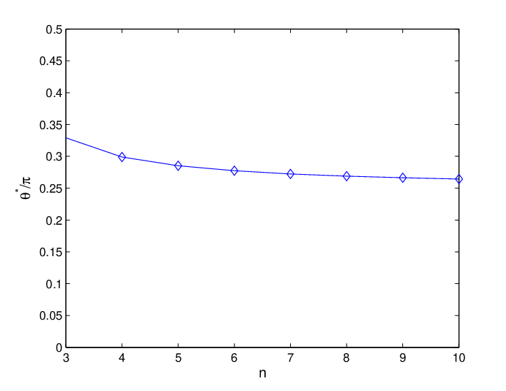
Refer to caption
Figure 10: (Color online) The possible values θ\theta with θ<θ∗\theta<\theta^{*} for verifying the genuinely nn-partite nonlocality of nn-partite maximal slice (MS) state.

Example S9. Consider a generalized tripartite entangled pure state AAC:

|Φ3⟩=γ0​|000⟩+γ1​ei​ϕ​|100⟩+γ2​|101⟩+γ3​|110⟩+γ4​|111⟩\displaystyle|\Phi_{3}\rangle=\gamma_{0}|000\rangle+\gamma_{1}e^{i\phi}|100\rangle+\gamma_{2}|101\rangle+\gamma_{3}|110\rangle+\gamma_{4}|111\rangle (E49)

where ϕ∈[0,π],γi≥0,∑iγi2=1,γ0≠0,γ2+γ4≠0,γ3+γ4≠0\phi\in[0,\pi],\gamma_{i}\geq 0,\sum_{i}\gamma_{i}^{2}=1,\gamma_{0}\not=0,\gamma_{2}+\gamma_{4}\not=0,\gamma_{3}+\gamma_{4}\not=0. Define Ai=σzA_{i}=\sigma_{z} for all iis. It follows that

ω2​-pr​(|Φ3⟩)=\displaystyle\omega_{2\mbox{\small-pr}}(|\Phi_{3}\rangle)= 2​γ02+2​γ42−23​(γ12+γ22+γ32)−49​(3​γ02+γ12−γ22−γ32−γ42)2\displaystyle 2\gamma_{0}^{2}+2\gamma_{4}^{2}-\frac{2}{3}(\gamma_{1}^{2}+\gamma_{2}^{2}+\gamma_{3}^{2})-\frac{4}{9}(3\gamma_{0}^{2}+\gamma_{1}^{2}-\gamma_{2}^{2}-\gamma_{3}^{2}-\gamma_{4}^{2})^{2}
>\displaystyle> 1\displaystyle 1 (E50)

which violates the inequality (E32) when γi\gamma_{i} satisfy the inequality: γ02+γ42>12\gamma_{0}^{2}+\gamma_{4}^{2}>\frac{1}{2} and 3​γ02+γ12=γ22+γ32+γ423\gamma_{0}^{2}+\gamma_{1}^{2}=\gamma_{2}^{2}+\gamma_{3}^{2}+\gamma_{4}^{2}. i.e., γ02=16−13​γ12,γ42=12−γ22−γ32\gamma_{0}^{2}=\frac{1}{6}-\frac{1}{3}\gamma_{1}^{2},\gamma_{4}^{2}=\frac{1}{2}-\gamma_{2}^{2}-\gamma_{3}^{2} and γ22+γ32+13​γ12≤16\gamma_{2}^{2}+\gamma_{3}^{2}+\frac{1}{3}\gamma_{1}^{2}\leq\frac{1}{6}.

E3. Mixed entangled states

Consider the nn-partite Werner state Werner:

ρ=vn​|Φ⟩​⟨Φ|+1−vn2n​𝟙2n\displaystyle\rho=v_{n}|\Phi\rangle\langle\Phi|+\frac{1-v_{n}}{2^{n}}\mathbbm{1}_{2^{n}} (E51)

where |Φ⟩|\Phi\rangle is any nn-partite qubit state on Hilbert space ℍ1⊗⋯⊗ℍn\mathbb{H}_{1}\otimes\cdots\otimes\mathbb{H}_{n}, and 𝟙2n\mathbbm{1}_{2^{n}} is the identity operator, vn∈[0,1]v_{n}\in[0,1] is a noise parameter. For a positive semidefinite operator of ρ\rho we have

ρ1/2=\displaystyle\rho^{1/2}= gv​|Φ⟩​⟨Φ|+1−vn2n​𝟙2n\displaystyle g_{v}|\Phi\rangle\langle\Phi|+\sqrt{\frac{1-v_{n}}{2^{n}}}\mathbbm{1}_{2^{n}} (E52)

with gv=vn+1−vn2n−1−vn2ng_{v}=\sqrt{v_{n}+\frac{1-v_{n}}{2^{n}}}-\sqrt{\frac{1-v_{n}}{2^{n}}}. The nonlinear functionals fif_{i}s can be then rewritten into

f1​(ρ,Ai)=gv2​⟨Φ|Ai|Φ⟩2+2​gv​1−vn2n​⟨Φ|Ai|Φ⟩−vn+1\displaystyle f_{1}(\rho,A_{i})=g_{v}^{2}\langle\Phi|A_{i}|\Phi\rangle^{2}+2g_{v}\sqrt{\frac{1-v_{n}}{2^{n}}}\langle\Phi|A_{i}|\Phi\rangle-v_{n}+1 (E53)
f2​(ρ,Ai,Aj)=gv2​⟨Φ|Ai|Φ⟩​⟨Φ|Aj|Φ⟩+2​gv​1−v2n​⟨Φ​|Ai⊗Aj|​Φ⟩\displaystyle f_{2}(\rho,A_{i},A_{j})=g_{v}^{2}\langle\Phi|A_{i}|\Phi\rangle\langle\Phi|A_{j}|\Phi\rangle+2g_{v}\sqrt{\frac{1-v}{2^{n}}}\langle\Phi|A_{i}\otimes{}A_{j}|\Phi\rangle (E54)

for p=12p=\frac{1}{2}. It follows from Eqs.(E53), (E54) and (E32) that

∑1≤i≠j≤n(1n−2​(n−1)​gvn2​vn​1−vn2n)​⟨Ai​Aj⟩ρ−n−1n2​gv2vn2​(∑i=1n⟨Ai⟩ρ)2\displaystyle\sum_{1\leq i\not=j\leq n}(\frac{1}{n}-\frac{2(n-1)g_{v}}{n^{2}v_{n}}\sqrt{\frac{1-v_{n}}{2^{n}}})\langle{}A_{i}A_{j}\rangle_{\rho}-\frac{n-1}{n^{2}}\frac{g_{v}^{2}}{v_{n}^{2}}(\sum_{i=1}^{n}\langle{}A_{i}\rangle_{\rho})^{2}
−2​(n−1)​gvn2​vn​1−vn2n​⟨Ai⟩ρ−(nn−1)​(1−vn)n≤k−1\displaystyle-\frac{2(n-1)g_{v}}{n^{2}v_{n}}\sqrt{\frac{1-v_{n}}{2^{n}}}\langle{}A_{i}\rangle_{\rho}-\frac{(n_{n}-1)(1-v_{n})}{n}\leq k-1 (E55)

for any kk-producible state ρ\rho. Note that the noise parameter is involved in the left side of the inequality (E55). Hence, it should be computed firstly in applications.
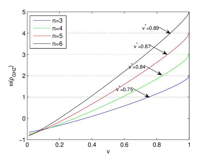
Refer to caption
Figure 11: (Color online) vn∗v^{*}_{n} denotes the critical noise parameter vv for verifying the genuinely nn-partite nonlocality of Werner state ρG​H​Z\rho_{GHZ} in the biseparable model Sy, n=3,⋯,6n=3,\cdots,6.

Example S10. Consider an nn-partite GHZ state: |Φ⟩=12​(|0⟩⊗n+|1⟩⊗n)|\Phi\rangle=\frac{1}{\sqrt{2}}(|0\rangle^{\otimes n}+|1\rangle^{\otimes n}). Define Ai=σzA_{i}=\sigma_{z} for all ii. It follows that ⟨Ai⟩ρG​H​Z=0\langle{}A_{i}\rangle_{\rho_{GHZ}}=0, and ⟨Ai⊗Aj⟩ρG​H​Z=vn\langle{}A_{i}\otimes{}A_{j}\rangle_{\rho_{GHZ}}=v_{n} for all ii and j≠ij\not=i. From Eqs.(E51) and (E55) we get that

ωk​-pr​(ρG​H​Z)=\displaystyle\omega_{k\mbox{\small-pr}}(\rho_{GHZ})= ∑i≠j(1n−2​(n−1)​gvn2​vn​1−vn2n)​⟨Ai⊗Aj⟩ρG​H​Z−n−1n2​gv2vn2​(∑i=1n⟨Ai⟩ρG​H​Z)2\displaystyle\sum_{i\not=j}(\frac{1}{n}-\frac{2(n-1)g_{v}}{n^{2}v_{n}}\sqrt{\frac{1-v_{n}}{2^{n}}})\langle{}A_{i}\otimes{}A_{j}\rangle_{\rho_{GHZ}}-\frac{n-1}{n^{2}}\frac{g_{v}^{2}}{v_{n}^{2}}(\sum_{i=1}^{n}\langle{}A_{i}\rangle_{\rho_{GHZ}})^{2}
−2​(n−1)​gvn2​vn​1−vn2n​⟨Ai⟩ρG​H​Z−(n−1)​(1−vn)n\displaystyle-\frac{2(n-1)g_{v}}{n^{2}v_{n}}\sqrt{\frac{1-v_{n}}{2^{n}}}\langle{}A_{i}\rangle_{\rho_{GHZ}}-\frac{(n-1)(1-v_{n})}{n}
=\displaystyle= vn​(n−1)−2​(n−1)2​gvn​1−vn2n−(n−1)​(1−vn)n\displaystyle v_{n}(n-1)-\frac{2(n-1)^{2}g_{v}}{n}\sqrt{\frac{1-v_{n}}{2^{n}}}-\frac{(n-1)(1-v_{n})}{n}
>\displaystyle> k−1\displaystyle k-1 (E56)

which violates the inequality (E55) when vn>vn∗v_{n}>v^{*}_{n}. Numeric evaluations of vv are shown in Figure S11.

Example S11. Consider a tripartite maximally entangled W state: |Φ⟩=13​(|001⟩+|010⟩+|100⟩)|\Phi\rangle=\frac{1}{\sqrt{3}}(|001\rangle+|010\rangle+|100\rangle). Define Ai=σxA_{i}=\sigma_{x} for all iis. It is easy to check ⟨Ai⟩ρW=0\langle{}A_{i}\rangle_{\rho_{W}}=0, and ⟨Ai⊗Aj⟩ρW=2​v33\langle{}A_{i}\otimes{}A_{j}\rangle_{\rho_{W}}=\frac{2v_{3}}{3} for all iis and j≠ij\not=i. From Eqs.(E51) and (E55) we get that

ω2​-pr​(ρW)=\displaystyle\omega_{2\mbox{\small-pr}}(\rho_{W})= ∑i≠j(13−4​gv9​v3​1−v38)​⟨Ai​Aj⟩ρW−29​gv2v32​(∑i=13⟨Ai⟩ρW)2\displaystyle\sum_{i\not=j}(\frac{1}{3}-\frac{4g_{v}}{9v_{3}}\sqrt{\frac{1-v_{3}}{8}})\langle{}A_{i}A_{j}\rangle_{\rho_{W}}-\frac{2}{9}\frac{g_{v}^{2}}{v_{3}^{2}}(\sum_{i=1}^{3}\langle{}A_{i}\rangle_{\rho_{W}})^{2}
−4​gv9​vn​1−vn8​⟨Ai⟩ρW−2​(1−vn)3\displaystyle-\frac{4g_{v}}{9v_{n}}\sqrt{\frac{1-v_{n}}{8}}\langle{}A_{i}\rangle_{\rho_{W}}-\frac{2(1-v_{n})}{3}
=\displaystyle= 4​v33−16​gv9​1−v38−2​(1−v3)3\displaystyle\frac{4v_{3}}{3}-\frac{16g_{v}}{9}\sqrt{\frac{1-v_{3}}{8}}-\frac{2(1-v_{3})}{3}
>\displaystyle> 1\displaystyle 1 (E57)

which violates the inequality (E55) for k=2k=2 when v3>v3∗v_{3}>v^{*}_{3}, where gv=v3+1−v38−1−v38g_{v}=\sqrt{v_{3}+\frac{1-v_{3}}{8}}-\sqrt{\frac{1-v_{3}}{8}}. Numeric evaluations of vv are shown in Figure S12.

Refer to caption
Figure 12: (Color online) v∗v^{*} denotes the critical noise parameter vv for verifying the genuinely tripartite nonlocality of Werner state ρW\rho_{W}.

References

  • (1) G. Svetlichny, Distinguishing three-body from two-body nonseparability by a Bell-type inequality, Phys. Rev. D 35, 3066 (1987).
  • (2) D. M. Greenberger, M. A. Horne, A. Zeilinger, in Bell’s Theorem, Quantum Theory and Conceptions of the Universe, edited by M. Kafatos, Kluwer, Dordrecht, 1989.
  • (3) W. Dür, G. Vidal, and J. I. Cirac, Three qubits can be entangled in two inequivalent ways, Phys. Rev. A 62, 062314 (2000).
  • (4) E. P. Wigner and M. M. Yanase, Information contents of distributions, PNAS 49, 910 (1963).
  • (5) E. H. Lieb, Convex trace functions and the Wigner-Yanase-Dyson conjecture, Adv. Math. 1, 267-288 (1973).
  • (6) S. Ghose, N. Sinclair, S. Debnath, P. Rungta, & R. Stock, Tripartite entanglement versus tripartite nonlocality in three-qubit Greenberger-Horne-Zeilinger-class states, Phys. Rev. Lettt. 102, 250404 (2009).
  • (7) A. Acín, A. Andrianov, L. Costa, E. Jané, I. Latorre, and R. Tarrach, Generalized Schmidt decomposition and classification of three-quantum-bit states, Phys. Rev. Lett. 85, 1560 (2000).
  • (8) R. F. Werner, Quantum states with Einstein-Podolsky-Rosen correlations admitting a hidden-variable model, Phys. Rev. A 40, 4277 (1989).
  • (9) D. P. Bertsekas, Constrained optimization and Lagrange multiplier methods, Academic press, 2014.