Quantum steering as a witness of quantum scrambling
Abstract
Quantum information scrambling describes the delocalization of local information to global information in the form of entanglement throughout all possible degrees of freedom. A natural measure of scrambling is the tripartite mutual information (TMI), which quantifies the amount of delocalized information for a given quantum channel with its state representation, i.e., the Choi state. In this work, we show that quantum information scrambling can also be witnessed by temporal quantum steering for qubit systems. We can do so because there is a fundamental equivalence between the Choi state and the pseudo-density matrix formalism used in temporal quantum correlations. In particular, we propose a quantity as a scrambling witness, based on a measure of temporal steering called temporal steerable weight. We justify the scrambling witness for unitary qubit channels by proving that the quantity vanishes whenever the channel is non-scrambling.
I Introduction.
Quantum systems evolving under strongly interacting channels can experience the delocalization of initially local information into non-local degrees of freedom. Such an effect is termed “quantum information scrambling,” and this new way of looking at delocalization in quantum theory has found applications in a range of physical effects, including chaos in many-body systems (Maldacena and Stanford 2016; Nahum et al. 2017; von Keyserlingk et al. 2018; Cotler et al. 2017; Fan et al. 2017; Khemani et al. 2018; Page 1993; Khemani et al. 2018; Gu et al. 2017), and the black-hole information paradox (Hayden and Preskill 2007; Sekino and Susskind 2008; Lashkari et al. 2013; Gao et al. 2017; Shenker and Stanford 2014a; Maldacena et al. 2017; Roberts et al. 2015; Shenker and Stanford 2014b; Roberts and Stanford 2015; Blake 2016; Kitaev 2014).
One can analyze the scrambling effect by using the state representation of a quantum channel (also known as the Choi state), which encodes the input and output of a quantum channel into a quantum state (Choi 1975; Jamiołkowski 1972). Within this formulation, quantum information scrambling can be measured by the tripartite mutual information (TMI) of a Choi state Hosur et al. 2016; Ding et al. 2016; Seshadri et al. 2018; Iyoda and Sagawa 2018; Shen et al. 2020; Li et al. 2020; Pappalardi et al. 2018 which is written as
| (1) |
Here, denotes a local region of the input subsystem whereas and are partitions of the output subsystem. The mutual information quantifies the amount of information about stored in the region . When or , it means that the amount of information about encoded in the whole output region is larger than that in local regions and . Therefore, implies the delocalization of information or quantum information scrambling Hosur et al. 2016. Note that the TMI and the out-of-time-ordered correlator are closely related, suggesting that one can also use the out-of-time-ordered correlator as an alternative witness of quantum information scrambling (Hosur et al. 2016; Landsman et al. 2019; Swingle et al. 2016; Yao et al. 2016; Zhu et al. 2016; Gärttner et al. 2017; Swingle and Yunger Halpern 2018; Huang et al. 2019; Yoshida and Yao 2019; González Alonso et al. 2019).
From another point of view, because TMI is a multipartite entanglement measure, Eq. (1) can also be seen as a quantification of the multipartite entanglement in time, i.e., the entanglement between input and output subsystems Hosur et al. 2016. Motivated by such an insight, one could expect that the scrambling effect can also be investigated from the perspective of temporal quantum correlations, i.e., temporal analogue of space-like quantum correlations.
Moreover, Ku et al. (Ku et al. 2018) has shown that three notable temporal quantum correlations (temporal nonlocality, temporal steering, and temporal inseperability) can be derived from a fundamental object called pseudo-density matrix (Fitzsimons et al. 2015; Ried et al. 2015; Zhao et al. 2018; Pisarczyk et al. 2019a), while elsewhere it was noted that there is a strong relationship between the Choi state and the pseudo-density matrix itself (Pisarczyk et al. 2019b). Taking inspiration from these connections, in this work, we aim to link the notion of scrambling to one particular scenario of temporal quantum correlation called temporal steering (TS) (Chen et al. 2014; Chen et al. 2015; Chen et al. 2016; Ku et al. 2016; Ku et al. 2018; Chen et al. 2017; Bartkiewicz et al. 2016; Liu et al. 2018).
Partly inspired by the Leggett-Garg inequality (Leggett and Garg 1985; Emary et al. 2013), temporal steering was developed as a temporal counterpart of the notion of spatial EPR steering (Schrödinger 1936; Wiseman et al. 2007; Jones et al. 2007; Cavalcanti et al. 2009; Piani and Watrous 2015; Skrzypczyk et al. 2014; Costa and Angelo 2016; Branciard et al. 2012; Law et al. 2014; Uola et al. 2020). Recent work has shown that TS can quantify the information flow between different quantum systems (Chen et al. 2016), further suggesting it may also be useful in the study of scrambling. Here, our goal is to demonstrate that one can witness information scrambling with temporal steering, which implies that the scrambling concept has nontrivial meaning in the broader context of temporal quantum correlations. In addition, we wish to show that one can use “measures” developed to study temporal steering as a practical tool for the study of scrambling.
We will restrict our attention to unitary channels of qubit systems, where the structure of non-scrambling channels can be well characterized Ding et al. 2016. More specifically, a unitary channel is non-scrambling, i.e. , if and only if the unitary is a “criss-cross” channel that locally routes the local information from the input to the output subsystems. For qubit systems, a criss-cross channel can be described by a sequence of local unitaries and SWAP operations.
The main result of this work is that we propose a quantity, , as a scrambling witness based on a measure of temporal steering called temporal steerable weight. We justify to be a scrambling witness by proving that when the global unitary channel is non-scrambling as mentioned above. We then compare the with by numerically simulating the Ising spin-chain model and the Sachdev-Ye-Kitaev (SYK) model. Finally, based on the one-sided device independent nature of steering, we point out that obtaining requires less experimental resource than .

II Extended temporal steering scenario and scrambling witness
II.1 Temporal steering scenario
Let us review the TS scenario Chen et al. 2014 with the schematic illustration shown in Fig. 1. We focus on the reduced system and treat other qubits as the environment. In general, the TS task consists of many rounds of experiments. For each round, Alice receives with a fixed initial state . Before the system evolves, Alice performs one of the projective measurements on . Here, stands for the index of the measurement basis, to which Alice can freely choose, and is the corresponding measurement outcome. The resulting post-measured conditional states can be written as
| (2) |
where predicts the probability of obtaining the outcome conditioned on Alice’s choice . Alice then sends the system to Bob through the quantum channel , which describes the reduced dynamics of alone by tracing out other qubits. Finally, Bob performs another measurement on after the evolution.
After all rounds of the experiments are finished, Alice sends her measurement results to Bob by classical communication, such that, Bob can also obtain the probability distribution . Additionally, based on the knowledge for each round of the experiment, Bob can approximate the conditional state by quantum state tomography. The aforementioned probability distribution and the conditional states can be summarized as a set called the TS assemblage . Note that the assemblage can also be derived from the pseudo-density matrix (see Appendix A for the derivation). In Appendix A, we also show that the Choi matrix and the pseudo-density matrix are related by a partial transposition.
Now, Bob can determine whether a given assemblage is steerable or unsteerable; that is, whether his system is quantum mechanically steered by Alice’s measurements. In general, if the assemblage is unsteerable, it can be generated in a classical way, which is described by the local hidden state model:
| (3) |
where is an ensemble of local hidden states, and stands for classical post-processing. Therefore, the assemblage is steerable when it cannot be described by Eq. (3).
Bob can further quantify the magnitude of temporal steering Cavalcanti and Skrzypczyk 2016; Uola et al. 2020. Here, we use one of the quantifiers called temporal steerable weight (TSW) Chen et al. 2016. For a given TS assemblage , one can decompose it into a mixture of a steerable and unsteerable parts, namely,
| (4) |
where and are the steerable and unsteerable assemblages, respectively, and stands for the portion (or weight) of the unsteerable part with . The TSW for the assemblage is then defined as
| (5) |
where is the maximal unsteerable portion among all possible decompositions described by Eq. (4). In other words, TSW can be interpreted as the minimum steerable resource required to reproduce the TS assemblage (e.g., for minimal steerability, and for maximal steerability). Note that Eq. (5) can be numerically computed through semi-definite programming (Cavalcanti and Skrzypczyk 2016).
According to Ref. Chen et al. 2016, the TSW can reveal the direction of the information flow between an open quantum system and its environment during the time evolution. When the information irreversibly flows out to the environment, TSW will monotonically decrease. Accordingly, the temporal increase of TSW implies information backflow. Recall that Alice steers ’s time evolution by her measurement . In other words, the measurement encodes the information about in . Therefore, after the evolution, Bob can estimate the amount of the information preserved in by computing the TSW.
II.2 Extended temporal steering as a witness of scrambling
As shown in Fig. 1, the evolution for the total system is still unitary, meaning that the information initially stored in is just redistributed (and localized) or scrambled after the evolution. Therefore, if we extend the notion of TS, which allows Bob to access the full system (regions and ), he can, in general, find out how the information localized or scrambled throughout the whole system. To be more specific, we now consider a global system with qubits labeled by . Before Alice performs any measurement, we reset the total system by initializing the qubits in the maximally mixed state , where is the two-dimensional identity matrix. In this case, no matter how one probes the system, it gives totally random results, and no meaningful information can be learned. Then, Alice encodes the information in by performing , which results in the conditional states of the total system:
| (6) | ||||
| with | (7) |
After that, let these conditional states evolve freely to time , such that
| (8) |
where can be any unitary operator acting on the total system. The assemblage for the global system then reads
| (9) |
Because the global evolution is unitary, it is straightforward that
| (10) |
which means that the information is never lost when all the degrees of freedom in the global system can be accessed by Bob.
In order to know how the information spread throughout all degrees of freedom, Bob can further analyze the assemblages obtained from different portions of the total system. For instance, he can divide the whole system into two local regions and as shown in Fig. 1, where contains qubits and contains qubits , such that Bob obtains two additional assemblages: and . Therefore, he can compute and , estimating the amount of information localized in regions C and D.
In analogy with Eq. (1), we propose the following quantity to be a scrambling witness:
| (11) |
where the minus sign for the quantity aims to keep the consistency with the TMI scrambling measure in Eq. (1). It can be interpreted as the information stored in the whole system minus the information localized in regions and ; namely, the information scrambled to the non-local degrees of freedom.
As mentioned in the introduction section, for a non-scrambling channel consisting of local unitaries and SWAP operations, the information will stay localized (non-scrambled). Therefore, we further justify that can be a scrambling witness, under the assumption of global unitary evolution, by proving that under non-scrambling evolutions, this quantity will vanish, i.e. . Accordingly, any nonzero value of can be seen as a witness of scrambling.
Theorem 1.
If the global unitary evolution is local for regions and , that is, , the resulting is zero.
The proof is given in Appendix B.
Theorem 2.
If the global unitary is a SWAP operation between qubits, then .
The proof is given in Appendix C.
III numerical simulations
In this section, we present the numerical simulations for the Ising spin chain and the SYK model. For simplicity, we consider to be projectors of Pauli matrices such that Chen et al. 2016.
III.1 Example 1: The Ising spin chain


We now consider a one-dimensional Ising model of qubits with the Hamiltonian
| (12) |
The key feature is that one can obtain chaotic behavior by simply turning on the longitudinal field parametrized by .
Here, we consider the system containing 7 qubits and compare the dynamical behavior of information scrambling for chaotic (, ) and integrable regimes (, ) by encoding the information in .
As shown in Fig. 2, we plot the information scrambling measured by and witnessed by and the amount of information stored in region () with the quantities and TSW [ and TSW] for different partitions of the output system. For a fixed output partition, [Fig. 2(a3), 2(b3), 2(c3) for instance], one can find that the local minima of the scrambling corresponds to the local maxima of the information stored either in region or region . Therefore, we can conclude that the decrease of the scrambling during the evolution results from the information backflow from non-local degrees of freedom to local degrees of freedom.
Moreover, information scrambling behaves differently for chaotic and integrable evolutions. For chaotic evolution, the scrambling will remain large after a period of time, because the information is mainly encoded in non-local degrees of freedom. However, for integrable systems, we can observe that both and show oscillating behavior. Furthermore, as the dimension of region becomes larger, the oscillating behavior of the scrambling for integrable cases significantly increases, whereas the scrambling patterns for chaotic cases remain unchanged.
III.2 Example 2 : The Sachdev-Ye-Kitaev model
We now consider the SYK model which can be realized by a Majorana fermionic system with the Hamiltonian
| (13) | |||
where the represent Majorana fermions with . Meanwhile, in the Hamiltonian follow the random normal distribution with zero mean and variance . To study this model in qubit system, we can use the Jordan-Wigner transformation
| (14) |
to convert the Majorana fermions to spin chain Pauli operators. In our numerical results, we consider (a seven qubits system) and . Figure 3 shows the time evolutions of the information scrambling and the information localized in region and for different partitions of the output system similar to those in Example .
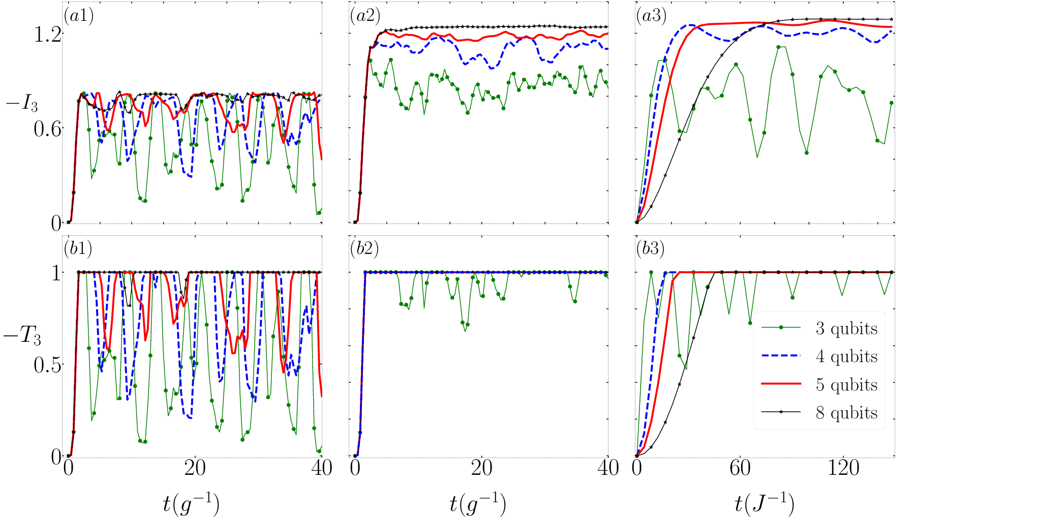
The main difference between these examples is that, in Example , the qubits only interact with their nearest neighbors; whereas in example , the model includes the interactions to all other qubits. Therefore, we can observe that in the spin chain model, the scrambling is sensitive to the dimension of the output system. However, in the SYK model, the scrambling is not susceptible to the partition of the output system, namely, the scrambling time and the magnitude of the tripartite mutual information after the scrambling period of different output partitions are similar (asymptotically reaching the Harr-scrambled value Hosur et al. 2016). Note that in Appendix E, we also provide numerical simulations involving different number of qubits for the above examples. We find that when decreasing (increasing) the number of qubits, the tendency of information backflow Chen et al. 2016 from global to local degrees of freedom will increase (decrease) for both chaotic and integrable dynamics.
Finally, for the scrambling dynamics (chaotic spin chain and SYK model), we can find that degrades more quickly to zero than . In addition, remains zero all the time, while could reach some non-zero value. The different behavior between the and results from the hierarchical relation between these two quantities (Ku et al. 2018), which states that temporal quantum steering is a stricter quantum correlation than bipartite mutual information. In other words, we can find some moments where has non-zero value whereas is zero, but not vice versa. The situation when [] implies that [] reaches its maximum. Therefore, for scrambling dynamics we can observe that reaches its maximum earlier than .
IV Summary
| Space-like structure | Time-like structure | |
| Diagram | ||
![[Uncaptioned image]](2003.07043v3/Space-like.png) |
![[Uncaptioned image]](2003.07043v3/time-like.png) | |
| Operator | Choi Matrix | Pseudo Density Matrix |
| Quantum correlations | Mutual information Entanglement CHSH inequality | Temporal steering Temporal inseparability Legget-Garg inequality |
| Input state | EPR pairs | Maximally mixed states |
In summary, we demonstrate that the information scrambling can not only be verified by the spatial quantum correlations encoded in a Choi matrix but also the temporal quantum correlations encoded in a pseudo-density matrix (see Table 1 for the comparison between the space-like and time-like structures). Moreover, we further provide an information scrambling witness, , based on the extended temporal steering scenario.
A potential advantage of using as a scrambling witness, over , is that requires less measurement resources than . More specifically, when measuring , we do not have to access the full quantum state of the input region , because in the steering scenario Alice’s measurement bases are only characterized by the classical variable . From a practical point of view, the number of Alice’s measurement basis can be less than that required for performing quantum state tomography on the region . For the examples presented in this work, we consider that region only contains a single qubit (), in which the standard choice of the measurement bases is the set of Pauli matrices, . For the steering scenario, we can choose only two of these matrices as Alice’s measurement bases, though for the numerical simulations presented in this work, we still consider that all three Pauli matrices are used by Alice.
Once the dimension of region increases, the number of the measurements required to perform quantum state tomography and obtain will also increase. However, as aforementioned, for the steering scenario, the dimension of the region is not assumed, implying that we can still choose a manageable number of Alice’s measurements to verify the steerability and compute .
Finally, it is important to note that we only claim that is a witness of scrambling rather than a quantifier, because we only prove that vanishes whenever the evolution is non-scrambling. An open question immediately arises: Can be further treated as a quantifier from the viewpoint of resource theory (Chitambar and Gour 2019)? To show this, our first step would be to prove that monotonically decreases whenever the evolution is non-scrambling, and we leave it as a future work.
Note added—After this work was completed, we became aware of (Zhang et al. 2020), which independently showed that the temporal correlations are connected with information scrambling, because the out-of-time-ordered correlators can be calculated from pseudo-density matrices.
Acknowledgements.
This work is supported partially by the National Center for Theoretical Sciences and Ministry of Science and Technology, Taiwan, Grants No. MOST 107-2628-M-006-002-MY3, and MOST 109-2627-M-006 -004, and the Army Research Office (under Grant No. W911NF-19-1-0081). N.L. acknowledges partial support from JST PRESTO through Grant No. JPMJPR18GC, the Foundational Questions Institute (FQXi), and the NTT PHI Laboratory. F.N. is supported in part by: Nippon Telegraph and Telephone Corporation (NTT) Research, the Japan Science and Technology Agency (JST) [via the Quantum Leap Flagship Program (Q-LEAP), the Moonshot R&D Grant Number JPMJMS2061, and the Centers of Research Excellence in Science and Technology (CREST) Grant No. JPMJCR1676], the Japan Society for the Promotion of Science (JSPS) [via the Grants-in-Aid for Scientific Research (KAKENHI) Grant No. JP20H00134 and the JSPS–RFBR Grant No. JPJSBP120194828], the Army Research Office (ARO) (Grant No. W911NF-18-1-0358), the Asian Office of Aerospace Research and Development (AOARD) (via Grant No. FA2386-20-1-4069), and the Foundational Questions Institute Fund (FQXi) via Grant No. FQXi-IAF19-06.Appendix A Relation between Choi matrix and pseudo density matrix
To illustrate the main idea behind the TMI scrambling measure in Ref. (Hosur et al. 2016), let us now consider a system made up of qubits, labeled by , with a Hilbert space . We then create ancilla qubits, labeled with , where each is maximally entangled with the corresponding qubit . Therefore, the Hilbert space of the total qubits system is . The corresponding density operator is , where denotes the set of linear operators on the Hilbert state . We can expand with Pauli matrices such that
| (15) |
where , , and . Let us now send the original qubits into a quantum channel (completely positive and trance preserving map) . Here, we consider the channel to be unitary; namely, , where is a unitary operator. The evolved density matrix (known as the Choi matrix) then reads
| (16) |
In general, can be expanded as
| (17) |
We therefore can expand the Choi matrix into:
| . | (18) | ||||
We now construct the pseudo-density matrix (PDM) through a temporal analogue of quantum state tomography (QST) between measurement events at two different moments (Fitzsimons et al. 2015). A PDM for an qubits system in an initially maximally mixed state undergoing is given by
| (19) |
where is the expectation value of the product of the outcome of the measurement performed on the initial time and the outcome of the measurement performed at the final time . Similarly, .
By comparing the coefficients of the qubits Choi matrix () in Eq. (18) with those of the PDM in Eq. (19) (), one can find that these two matrices are related through a partial transposition of the input degree of freedom, i.e.
| (20) |
According to Ref. (Ku et al. 2018), the TS assemblage can also be derived from the pseudo density matrix [which is defined in Eq. (19)] by the following Born’s rule:
| (21) |
where denotes the partial trace over the input Hilbert space.
As mentioned in the main text, the notion of scrambling can be understood as the multipartite entanglement in the Choi state. Therefore, the insight inferred from Eq. (20) suggests us that it should be possible to reformulate the information scrambling with multipartite temporal quantum correlations.
Appendix B Proof of Theorem 1
Proof.
Let’s start from the evolved assemblage for the total system (region ):
| (22) | ||||
| (23) | ||||
| (24) |
Since and are unitary, leading to the invariance of the TSW, we find the following results:
| (25) | ||||
| (26) | ||||
| (27) |
It is straightforward to conclude that , since can be decomposed as the local hidden state model shown in Eq. (3). In addition,
| (28) |
for arbitrary positive integer . Therefore, we can deduce that
| (29) |
∎
Appendix C Proof of Theorem 2
Proof.
We can find that the sum of the TSW for regions and is invariant under any permutation between qubits such that
| (30) |
Therefore, under the SWAP operation, . ∎
Appendix D The qubit Clifford scrambler

In this section, we numerically analyze the qubit Clifford scrambling circuit, proposed in Ref. Landsman et al. 2019. The setting only involves three qubits with a quantum circuit depicted in Fig. 4, which is parametrized by . By changing the angle , one can scan the angle from non-scrambling () to maximally scrambling (), which can be described by the following unitary matrix
| (31) |
According to Ref. Landsman et al. 2019, the scrambling unitary delocalizes all single qubit Pauli operators to three qubit Pauli operators in the following way:
| (32) |
Such a delocalization is often known as operator growth, which can be viewed as a key signature of quantum scrambling. In Fig. 4, we plot the values of and by changing the angles . We can see that both and display an oscillating pattern with period . The value of reaches its maximum scrambling value at ; while, reaches its maximum scrambling value earlier than due to the sudden vanishing of the TSW for local regions.
Appendix E Numerical simulations for different system sizes
| 3-qubit | 4-qubit | 5-qubit | 8-qubit | |
|---|---|---|---|---|
| Spin chain(Integrable) | 5.295 | 2.602 | 1.764 | 0.557 |
| Spin chain(chaotic) | 1.945 | 0.692 | 0.266 | 0.038 |
| SYK model | 2.311 | 0.265 | 0.057 | 0.001 |
| 3-qubit | 4-qubit | 5-qubit | 8-qubit | |
|---|---|---|---|---|
| Spin chain(Integrable) | 7.589 | 4.240 | 2.894 | 0.329 |
| Spin chain(chaotic) | 1.340 | 0 | 0 | 0 |
| SYK model | 1.194 | 0 | 0 | 0 |
In Fig. 5, we plot the numerical simulations of and for the integrable spin chain, chaotic spin chain, and the SYK model, involving different numbers of qubits. We can observe that as the qubit number decreases (increases), the oscillation magnitude of information scrambling for both integrable and chaotic dynamics increases (decreases). The result suggests that when the system size decreases (increases), it would be more likely (unlikely) to observe information backflow from non-local to local degrees of freedom.
Because any decrease of () signifies the backflow of information, we can quantify the total amount of information backflow within a time interval by summing up the total negative changes of the scrambling witnesses. More specifically, we define a quantity , which quantifies the total amount of information backflow for a given time interval , as follows
| (33) |
where and . In other words, integrates all positive changes of (or equivalently, all negative changes of ) for . Note that this quantification of information backflow is consistent with that in the framework of quantum non-Markovianity (see Ref. Chen et al. 2016, for instance). We summarize the results in Table 2, which show that as the number of qubit increases, the amount of information backflow decreases, implying a stronger scrambling effect.
References
- Maldacena and Stanford (2016) J. Maldacena and D. Stanford, Remarks on the Sachdev-Ye-Kitaev model, Phys. Rev. D 94, 106002 (2016).
- Nahum et al. (2017) A. Nahum, J. Ruhman, S. Vijay, and J. Haah, Quantum Entanglement Growth under Random Unitary Dynamics, Phys. Rev. X 7, 031016 (2017).
- von Keyserlingk et al. (2018) C. W. von Keyserlingk, T. Rakovszky, F. Pollmann, and S. L. Sondhi, Operator Hydrodynamics, OTOCs, and Entanglement Growth in Systems without Conservation Laws, Phys. Rev. X 8, 021013 (2018).
- Cotler et al. (2017) J. Cotler, N. Hunter-Jones, J. Liu, and B. Yoshida, Chaos, complexity, and random matrices, J. High Energy Phys. 2017 (11), 48.
- Fan et al. (2017) R. Fan, P. Zhang, H. Shen, and H. Zhai, Out-of-time-order correlation for many-body localization, Science bulletin 62, 707 (2017).
- Khemani et al. (2018) V. Khemani, A. Vishwanath, and D. A. Huse, Operator Spreading and the Emergence of Dissipative Hydrodynamics under Unitary Evolution with Conservation Laws, Phys. Rev. X 8, 031057 (2018).
- Page (1993) D. N. Page, Average entropy of a subsystem, Phys. Rev. Lett. 71, 1291 (1993).
- Gu et al. (2017) Y. Gu, X.-L. Qi, and D. Stanford, Local criticality, diffusion and chaos in generalized Sachdev-Ye-Kitaev models, J. High Energy Phys. 2017 (5), 125.
- Hayden and Preskill (2007) P. Hayden and J. Preskill, Black holes as mirrors: quantum information in random subsystems, J. High Energy Phys. 2007 (09), 120.
- Sekino and Susskind (2008) Y. Sekino and L. Susskind, Fast scramblers, J. High Energy Phys. 2008 (10), 065.
- Lashkari et al. (2013) N. Lashkari, D. Stanford, M. Hastings, T. Osborne, and P. Hayden, Towards the fast scrambling conjecture, J. High Energy Phys. 2013 (4), 22.
- Gao et al. (2017) P. Gao, D. L. Jafferis, and A. C. Wall, Traversable wormholes via a double trace deformation, J. High Energy Phys. 2017 (12), 151.
- Shenker and Stanford (2014a) S. H. Shenker and D. Stanford, Black holes and the butterfly effect, J. High Energy Phys. 2014 (3), 67.
- Maldacena et al. (2017) J. Maldacena, D. Stanford, and Z. Yang, Diving into traversable wormholes, Fortschr. Phys. 65, 1700034 (2017).
- Roberts et al. (2015) D. A. Roberts, D. Stanford, and L. Susskind, Localized shocks, J. High Energy Phys. 2015 (3), 51.
- Shenker and Stanford (2014b) S. H. Shenker and D. Stanford, Multiple shocks, J. High Energy Phys. 2014 (12), 46.
- Roberts and Stanford (2015) D. A. Roberts and D. Stanford, Diagnosing chaos using four-point functions in two-dimensional conformal field theory, Phys. Rev. Lett. 115, 131603 (2015).
- Blake (2016) M. Blake, Universal charge diffusion and the butterfly effect in holographic theories, Phys. Rev. Lett. 117, 091601 (2016).
- Kitaev (2014) A. Kitaev, Hidden correlations in the Hawking radiation and thermal noise, in contribution to the Fundamental Physics Prize Symposium, Vol. 10 (2014).
- Choi (1975) M.-D. Choi, Completely positive linear maps on complex matrices, Linear Algebra Appl. 10, 285 (1975).
- Jamiołkowski (1972) A. Jamiołkowski, Linear transformations which preserve trace and positive semidefiniteness of operators, Rep. Math. Phys. 3, 275 (1972).
- Hosur et al. (2016) P. Hosur, X.-L. Qi, D. A. Roberts, and B. Yoshida, Chaos in quantum channels, J. High Energy Phys. 2016 (2), 4.
- Ding et al. (2016) D. Ding, P. Hayden, and M. Walter, Conditional mutual information of bipartite unitaries and scrambling, J. High Energy Phys. 2016 (12), 145.
- Seshadri et al. (2018) A. Seshadri, V. Madhok, and A. Lakshminarayan, Tripartite mutual information, entanglement, and scrambling in permutation symmetric systems with an application to quantum chaos, Phys. Rev. E 98, 052205 (2018).
- Iyoda and Sagawa (2018) E. Iyoda and T. Sagawa, Scrambling of quantum information in quantum many-body systems, Phys. Rev. A 97, 042330 (2018).
- Shen et al. (2020) H. Shen, P. Zhang, Y.-Z. You, and H. Zhai, Information scrambling in quantum neural networks, Phys. Rev. Lett. 124, 200504 (2020).
- Li et al. (2020) Y. Li, X. Li, and J. Jin, Information scrambling in a collision model, Phys. Rev. A 101, 042324 (2020).
- Pappalardi et al. (2018) S. Pappalardi, A. Russomanno, B. Žunkovič, F. Iemini, A. Silva, and R. Fazio, Scrambling and entanglement spreading in long-range spin chains, Phys. Rev. B 98, 134303 (2018).
- Landsman et al. (2019) K. A. Landsman, C. Figgatt, T. Schuster, N. M. Linke, B. Yoshida, N. Y. Yao, and C. Monroe, Verified quantum information scrambling, Nature 567, 61 (2019).
- Swingle et al. (2016) B. Swingle, G. Bentsen, M. Schleier-Smith, and P. Hayden, Measuring the scrambling of quantum information, Phys. Rev. A 94, 040302 (2016).
- Yao et al. (2016) N. Y. Yao, F. Grusdt, B. Swingle, M. D. Lukin, D. M. Stamper-Kurn, J. E. Moore, and E. A. Demler, Interferometric Approach to Probing Fast Scrambling, arXiv preprint arXiv:1607.01801 (2016).
- Zhu et al. (2016) G. Zhu, M. Hafezi, and T. Grover, Measurement of many-body chaos using a quantum clock, Phys. Rev. A 94, 062329 (2016).
- Gärttner et al. (2017) M. Gärttner, J. G. Bohnet, A. Safavi-Naini, M. L. Wall, J. J. Bollinger, and A. M. Rey, Measuring out-of-time-order correlations and multiple quantum spectra in a trapped-ion quantum magnet, Nat. Phys. 13, 781 (2017).
- Swingle and Yunger Halpern (2018) B. Swingle and N. Yunger Halpern, Resilience of scrambling measurements, Phys. Rev. A 97, 062113 (2018).
- Huang et al. (2019) Y. Huang, F. G. S. L. Brandão, and Y.-L. Zhang, Finite-size scaling of out-of-time-ordered correlators at late times, Phys. Rev. Lett. 123, 010601 (2019).
- Yoshida and Yao (2019) B. Yoshida and N. Y. Yao, Disentangling Scrambling and Decoherence via Quantum Teleportation, Phys. Rev. X 9, 011006 (2019).
- González Alonso et al. (2019) J. R. González Alonso, N. Yunger Halpern, and J. Dressel, Out-of-Time-Ordered-Correlator Quasiprobabilities Robustly Witness Scrambling, Phys. Rev. Lett. 122, 040404 (2019).
- Ku et al. (2018) H.-Y. Ku, S.-L. Chen, N. Lambert, Y.-N. Chen, and F. Nori, Hierarchy in temporal quantum correlations, Phys. Rev. A 98, 022104 (2018).
- Fitzsimons et al. (2015) J. F. Fitzsimons, J. A. Jones, and V. Vedral, Quantum correlations which imply causation, Sci. Rep. 5, 18281 (2015).
- Ried et al. (2015) K. Ried, M. Agnew, L. Vermeyden, D. Janzing, R. W. Spekkens, and K. J. Resch, A quantum advantage for inferring causal structure, Nat. Phys. 11, 414 (2015).
- Zhao et al. (2018) Z. Zhao, R. Pisarczyk, J. Thompson, M. Gu, V. Vedral, and J. F. Fitzsimons, Geometry of quantum correlations in space-time, Phys. Rev. A 98, 052312 (2018).
- Pisarczyk et al. (2019a) R. Pisarczyk, Z. Zhao, Y. Ouyang, V. Vedral, and J. F. Fitzsimons, Causal Limit on Quantum Communication, Phys. Rev. Lett. 123, 150502 (2019a).
- Pisarczyk et al. (2019b) R. Pisarczyk, Z. Zhao, Y. Ouyang, V. Vedral, and J. F. Fitzsimons, Causal limit on quantum communication, Physical review letters 123, 150502 (2019b).
- Chen et al. (2014) Y.-N. Chen, C.-M. Li, N. Lambert, S.-L. Chen, Y. Ota, G.-Y. Chen, and F. Nori, Temporal steering inequality, Phys. Rev. A 89, 032112 (2014).
- Chen et al. (2015) S.-L. Chen, C.-S. Chao, and Y.-N. Chen, Detecting the existence of an invisibility cloak using temporal steering, Sci. Rep. 5, 15571 (2015).
- Chen et al. (2016) S.-L. Chen, N. Lambert, C.-M. Li, A. Miranowicz, Y.-N. Chen, and F. Nori, Quantifying Non-Markovianity with Temporal Steering, Phys. Rev. Lett. 116, 020503 (2016).
- Ku et al. (2016) H.-Y. Ku, S.-L. Chen, H.-B. Chen, N. Lambert, Y.-N. Chen, and F. Nori, Temporal steering in four dimensions with applications to coupled qubits and magnetoreception, Phys. Rev. A 94, 062126 (2016).
- Chen et al. (2017) S.-L. Chen, N. Lambert, C.-M. Li, G.-Y. Chen, Y.-N. Chen, A. Miranowicz, and F. Nori, Spatio-temporal steering for testing nonclassical correlations in quantum networks, Sci. Rep. 7, 1 (2017).
- Bartkiewicz et al. (2016) K. Bartkiewicz, A. Černoch, K. Lemr, A. Miranowicz, and F. Nori, Temporal steering and security of quantum key distribution with mutually unbiased bases against individual attacks, Phys. Rev. A 93, 062345 (2016).
- Liu et al. (2018) B. Liu, Y. Huang, and Z. Sun, Quantum temporal steering in a dephasing channel with quantum criticality, Ann. Phys. 530, 1700373 (2018).
- Leggett and Garg (1985) A. J. Leggett and A. Garg, Quantum mechanics versus macroscopic realism: Is the flux there when nobody looks?, Phys. Rev. Lett. 54, 857 (1985).
- Emary et al. (2013) C. Emary, N. Lambert, and F. Nori, Leggett–Garg inequalities, Rep. Prog. Phys. 77, 016001 (2013).
- Schrödinger (1936) E. Schrödinger, Probability relations between separated systems, in Math. Proc. Cambridge Philos. Soc., Vol. 31 (Cambridge University Press, 1936) p. 446.
- Wiseman et al. (2007) H. M. Wiseman, S. J. Jones, and A. C. Doherty, Steering, Entanglement, Nonlocality, and the Einstein-Podolsky-Rosen Paradox, Phys. Rev. Lett. 98, 140402 (2007).
- Jones et al. (2007) S. J. Jones, H. M. Wiseman, and A. C. Doherty, Entanglement, Einstein-Podolsky-Rosen correlations, Bell nonlocality, and steering, Phys. Rev. A 76, 052116 (2007).
- Cavalcanti et al. (2009) E. G. Cavalcanti, S. J. Jones, H. M. Wiseman, and M. D. Reid, Experimental criteria for steering and the Einstein-Podolsky-Rosen paradox, Phys. Rev. A 80, 032112 (2009).
- Piani and Watrous (2015) M. Piani and J. Watrous, Necessary and Sufficient Quantum Information Characterization of Einstein-Podolsky-Rosen Steering, Phys. Rev. Lett. 114, 060404 (2015).
- Skrzypczyk et al. (2014) P. Skrzypczyk, M. Navascués, and D. Cavalcanti, Quantifying Einstein-Podolsky-Rosen Steering, Phys. Rev. Lett. 112, 180404 (2014).
- Costa and Angelo (2016) A. C. S. Costa and R. M. Angelo, Quantification of Einstein-Podolsky-Rosen steering for two-qubit states, Phys. Rev. A 93, 020103 (2016).
- Branciard et al. (2012) C. Branciard, E. G. Cavalcanti, S. P. Walborn, V. Scarani, and H. M. Wiseman, One-sided device-independent quantum key distribution: Security, feasibility, and the connection with steering, Phys. Rev. A 85, 010301 (2012).
- Law et al. (2014) Y. Z. Law, J.-D. Bancal, V. Scarani, et al., Quantum randomness extraction for various levels of characterization of the devices, J. Phys. A 47, 424028 (2014).
- Uola et al. (2020) R. Uola, A. C. S. Costa, H. C. Nguyen, and O. Gühne, Quantum steering, Rev. Mod. Phys. 92, 015001 (2020).
- Cavalcanti and Skrzypczyk (2016) D. Cavalcanti and P. Skrzypczyk, Quantum steering: a review with focus on semidefinite programming, Rep. Prog. Phys. 80, 024001 (2016).
- Chitambar and Gour (2019) E. Chitambar and G. Gour, Quantum resource theories, Reviews of Modern Physics 91, 025001 (2019).
- Zhang et al. (2020) T. Zhang, O. Dahlsten, and V. Vedral, Quantum correlations in time, arXiv preprint arXiv:2002.10448 (2020).