跳到论文正文
W Papers独立论文阅读器 arXiv:2003.07029 论文正文 计算阅读时间 · 0%
引用这篇论文根据当前论文元数据生成,正式投稿前建议核对。


License: arXiv.org perpetual non-exclusive license
arXiv:2003.07029v1 [cs.IT] 16 Mar 2020

Joint Power Allocation and Precoding for Network Coding based Cooperative Multicast Systems

Jun Li, and Wen Chen    Thanks: Jun˜Li and Wen˜Chen are with the Department of Electronic Engineering, Shanghai Jiaotong University, Shanghai, 200240 PRC. e-mail: {jleesr80, wenchen}@sjtu.edu.cn Thanks: This work is supported by NSF China #60672067, by NSF Shanghai #06ZR14041, by Shanghai-Canada NRC #06SN07112, by Cultivation Fund of the Key Scientific and Technical Innovation Project, Ministry of Education of China #706022, by Program for New Century Excellent Talents in University #NCET-06-0386, by PUJIANG Talents #07PJ4046, and by Huawei Fund for Sciences and Technologies in Universities #YJCB2008048WL
Abstract

In this letter, we propose two power allocation schemes based on the statistical channel state information (CSI) and instantaneous s→rs\rightarrow{r} CSI at transmitters respectively for a 2−N−22-N-2 cooperative multicast system with non-regenerative network coding. Then the isolated precoder and the distributed precoder are respectively applied to the schemes to further improve the system performance by achieving the full diversity gain. Finally, we demonstrate that joint instantaneous s→rs\rightarrow{r} CSI based power allocation and distributed precoder design achieve the best performance.

Index Terms: 
Cooperative multicast network, network coding, power allocation, precoder design, frame error probability.

I Introduction

Network coding has been proved to achieve the network multicast capacity bound in the wireline systems [1]. Recently, how to leverage network coding in wireless physical layer networks for system capacity improvement has drawn increasing interest [2]-[4]. However, these works are based on the multi-access relay channels model and unicast model.

In this letter, we study the multicast model with two sources, two destinations and NN relays (2−N−22-N-2 system) by following the second scheduling strategy in [5], where relays are arranged in the round-robin way. We suppose that s1s_{1} as well as s2s_{2} broadcast their information to the two destinations d1d_{1} and d2d_{2} simultaneously. From Fig. 1, we can see d1d_{1} (or d2d_{2}) is out of the transmission range of s2s_{2} (or s1s_{1}). The shared relays can help s1s_{1} (or s2s_{2}) reach their destinations. By the wireless network coding method, there are two time slots:
1. s1→{r,d1}s_{1}\rightarrow\{r,~d_{1}\} with Xs1X_{s_{1}}; s2→{r,d2}s_{2}\rightarrow\{r,~d_{2}\} with Xs2X_{s_{2}},
2. r→{d1,d2}r\rightarrow\{d_{1},~d_{2}\} with f⁡(Xs1,Xs2)f(X_{s_{1}},X_{s_{2}}),

Fig. 1: Multicast cooperative channels with NN relays.

where f⁡(⋅)f(\cdot) is certain mapping mechanism. We focus on the non-regenerative network coding where mixed signals are scaled and retransmitted to the destinations without decoding at relays. We propose two power allocation schemes based on the statistical channel state information (CSI) and the instantaneous s→rs\rightarrow{r} CSI at sources respectively. The isolated precoders and distributed precoders are respectively jointly working with the schemes to achieve the full diversity gain. We will demonstrate that the joint instantaneous s→rs\rightarrow{r} CSI based power allocation and distributed precoder can achieve the best performance against the other combinations in the terms of system frame error probability (SFEP).

II System Model

Channel coefficients are shown in Fig. 1 with zero means and unit variances. The noise variances are equal to σ2\sigma^{2} in all the receivers. To normalize the power, we denote PP as the average total network transmission power over a time slot. Then we define the system SNR as ρ≜Pσ2\rho\triangleq\frac{P}{\sigma^{2}}. We define xs≜[xs1,1,xs2,1,xs1,2,xs2,2,⋯,xs1,N,xs2,N]T\textbf{x}_{s}\triangleq[x_{s_{1},1},x_{s_{2},1},x_{s_{1},2},x_{s_{2},2},\cdots,x_{s_{1},N},x_{s_{2},N}]^{T} as a system frame which is composed of symbols from two sources. All symbols are equally probable from the QAM constellation set with zero means and variances 2​P2P. The symbol vector in the system frame for sk​(k=1, 2)s_{k}\,(k=1,\,2) is denoted as xsk=[xsk,1,xsk,2,⋯,xsk,N]T\textbf{x}_{s_{k}}=[x_{s_{k},1},x_{s_{k},2},\cdots,x_{s_{k},N}]^{T}. Since each relay is only used once during a frame period, we denote the signal received by the ii-th relay as yriy_{r_{i}}. The symbol vector received by the kk-th destination is denoted as ydk=[ydk,1,ydk,2,⋯,ydk,2​N−1,ydk,2​N]T\textbf{y}_{d_{k}}=[y_{d_{k},1},y_{d_{k},2},\cdots,y_{d_{k},2N-1},y_{d_{k},2N}]^{T}.

The total power consumed during a frame period is

ℰ⁡{k1T​|xs1|2+k2T​|xs2|2+|bT​yr|2}=2​N​P\mathcal{E}\left\{\textbf{k}_{1}^{T}|\textbf{x}_{s_{1}}|^{2}+\textbf{k}_{2}^{T}|\textbf{x}_{s_{2}}|^{2}+|\textbf{b}^{T}\textbf{y}_{r}|^{2}\right\}=2NP (1)

where yr=[yr1,yr2,⋯,yrN]T\textbf{y}_{r}=[y_{r_{1}},y_{r_{2}},\cdots,y_{r_{N}}]^{T}. The power is distributed according to the power allocation factor vectors, i.e., kk=[κk,1,⋯,κk,N]T\textbf{k}_{k}=[\kappa_{k,1},\cdots,\kappa_{k,N}]^{T} is the factor vector for the kk-th source and b=[b1,⋯,bN]T\textbf{b}=[b_{1},\cdots,b_{N}]^{T} is the amplification factor vector where bi=2​τi​P2​κ1,i​P+2​κ2,i​P+σ2b_{i}=\sqrt{\frac{2\tau_{i}{P}}{2\kappa_{1,i}{P}+2\kappa_{2,i}{P}+\sigma^{2}}} is the factor for the ii-th relay. Note that τi\tau_{i} is the corresponding power allocation factor for the ii-th relay. We denote t=[τ1,⋯,τN]T\textbf{t}=[\tau_{1},\cdots,\tau_{N}]^{T}.

The received signals of the kk-th destination for the (2​i−1)(2i-1)-th and 2​i2i-th time slots are respectively written as

ydk,2​i−1=ℏk​κk,i​xsk,i+vdk,2​i−1​,y_{d_{k},2i-1}=\hbar_{k}\sqrt{\kappa_{k,i}}x_{s_{k},i}+v_{d_{k},2i-1}\text{,}\qquad\qquad\qquad\qquad\;\; (2)
ydk,2​i=bi​hi,k​(g1,i​κ1,i​xs1,i+g2,i​κ2,i​xs2,i+vri)+vdk,2​i.\begin{split}y_{d_{k},2i}=b_{i}h_{i,k}(g_{1,i}\sqrt{\kappa_{1,i}}x_{s_{1},i}+g_{2,i}\sqrt{\kappa_{2,i}}x_{s_{2},i}+v_{r_{i}})+v_{d_{k},2i}.\end{split}

Note that vriv_{r_{i}} is the noise observed by the ii-th relay and vdk,2​iv_{d_{k},2i} is the noise observed by dkd_{k} in the 2​i2i-th time slot. Joint ML decoding is performed at the end of each frame period.

III Performance Analysis and Improvements

We measure the performance by system frame error probability (SFEP). We define that a frame is successfully transmitted if and only if both destinations can successfully receive the frame. So the SFEP of the multicast system is

Ps​y​s=Pdk​(1−Pdk¯)+Pdk¯​(1−Pdk)+Pdk​Pdk¯P_{sys}=P_{d_{k}}(1-P_{d_{\bar{k}}})+P_{d_{\bar{k}}}(1-P_{d_{k}})+P_{d_{k}}{P}_{d_{\bar{k}}} (3)

where k¯\bar{k} is the complementary element of kk in set {1,2}\{1,2\}, and PdkP_{d_{k}} is the FEP of dkd_{k}. We improve the performance by combining power allocation and precoders according to the knowledge of the CSI at sources.

III-A Statistical CSI based Power Allocation

Due to the symmetrical quality of Ps​y​sP_{sys} and according to the fact that each channel variance is equal, power should be equally allocated to each symbol of the two sources, i.e., k1=k2=[κ,⋯,κ]T\textbf{k}_{1}=\textbf{k}_{2}=[\kappa,\cdots,\kappa]^{T} and t=[τ,⋯,τ]T\textbf{t}=[\tau,\cdots,\tau]^{T}. Then the amplification factor b=2​τ​P4​κ​P+σ2b=\sqrt{\frac{2\tau{P}}{4\kappa{P}+\sigma^{2}}}. Then we get the statistical CSI based power allocation scheme as follows.

Theorem 1

When ρ\rho is large enough, the statistical CSI based optimal power allocation scheme chooses the power allocation factors as κ=12​(N+1)\kappa=\frac{1}{2(N+1)} and τ=NN+1\tau=\frac{N}{N+1}.             ❏

Proof: On the condition that only statistical CSI is available, PdkP_{d_{k}} can be deduced by the average pairwise error probability (PEP). Note that FEP=22​R​N​PEP\text{FEP}=2^{2RN}\text{PEP} since there are total 22​R​N2^{2RN} codewords, where RR is the transmission rate. So to find out the optimal relation between κ\kappa and τ\tau, we first come to the average PEP of the destinations. We rewrite (2) in matrix form as xdk=X2​N​h2​N+v2​N\textbf{x}_{d_{k}}=\textbf{X}_{2N}\textbf{h}_{2N}+\textbf{v}_{2N} and get the PEP by developing the method in [7].

PP​E,dk=P_{PE,d_{k}}=\qquad\qquad\qquad\qquad\qquad\qquad\qquad\qquad\qquad (4)
1π​∫0π2ℰh2​N​{exp⁡(−ρ​h2​NH​U2​NH​𝚺v−1​U2​N​h2​N8​sin2⁡θ)}​𝑑θ,\qquad\frac{1}{\pi}\int_{0}^{\frac{\pi}{2}}\mathcal{E}_{\textbf{h}_{2N}}\left\{\exp\left(-\rho\frac{\textbf{h}_{2N}^{H}\textbf{U}_{2N}^{H}{\boldsymbol{\Sigma}}_{\textbf{v}}^{-1}\textbf{U}_{2N}\textbf{h}_{2N}}{8\sin^{2}\theta}\right)\right\}\,\mathrm{d}{\theta},

where U2​N=X2​N−X^2​N\textbf{U}_{2N}=\textbf{X}_{2N}-\hat{\textbf{X}}_{2N} is the decoding error matrix and 𝚺v{\boldsymbol{\Sigma}}_{\textbf{v}} is the variance matrix of v2​N\textbf{v}_{2N}. h2​N\textbf{h}_{2N} can be written by T2​N​g2​N\textbf{T}_{2N}\textbf{g}_{2N} where g2​N=[ℏk,g1,1,g2,1,g1,2,g2,2,⋯,g1,N,g2,N]T\textbf{g}_{2N}=[\hbar_{k},g_{1,1},g_{2,1},g_{1,2},g_{2,2},\cdots,g_{1,N},g_{2,N}]^{T} and T2​N=diag⁡(1,b​h1,k,b​h1,k,b​h2,k,b​h2,k,⋯,b​hN,k,b​hN,k)\textbf{T}_{2N}=\mathrm{diag}(1,bh_{1,k},bh_{1,k},bh_{2,k},bh_{2,k},\cdots,bh_{N,k},bh_{N,k}). Note that for a random column vector z∼𝒩⁡(0,𝚺z)\textbf{z}\sim\mathcal{N}(0,\boldsymbol{\Sigma}_{\textbf{z}}) and a Hermitian matrix H, there is ℰ⁡[exp⁡(−zH​Hz)]=1/det(I+𝚺z​H)\mathcal{E}[\exp(-\textbf{z}^{H}\textbf{Hz})]=1/\det(\textbf{I}+\boldsymbol{\Sigma_{\textbf{z}}}\textbf{H}). We take expectation with respect to g2​N\textbf{g}_{2N} and let y=[y1,y2,⋯,yN]\textbf{y}=[y_{1},y_{2},\cdots,y_{N}] where yi=|hi,k|2y_{i}=|h_{i,k}|^{2} with the probability distribution function e−yie^{-{y_{i}}}. Then the PEP is written as

PP​E,dk=1π∫0π2∫0∞⋯∫0∞exp⁡(−∑j=1𝑁​yj)det(A)dydθ.P_{PE,d_{k}}=\frac{1}{\pi}\int_{0}^{\frac{\pi}{2}}\int_{0}^{\infty}\cdots\int_{0}^{\infty}\frac{\exp\left(-\overset{N}{\underset{j=1}{\boldsymbol{\sum}}}{y_{j}}\right)}{\det(\textbf{A})}\,\mathrm{d}{\textbf{y}}\,\mathrm{d}{\theta}. (5)

In (5), det(A)=det(A0)det(A1)⋯det(AN)\det(\textbf{A})=\det(\textbf{A}_{0})\det(\textbf{A}_{1})\cdots\det(\textbf{A}_{N}), where

A0=1+ρ8​sin2⁡θ​∑j=1𝑁​|usk,j|2,Ai=(1+λi​|us1,i|2λi​us1,i∗​us2,iλi​us1,i​us2,i∗1+λi​|us2,i|2),\begin{split}&\textbf{A}_{0}=1+\frac{\rho}{8\sin^{2}\theta}\overset{N}{\underset{j=1}{\boldsymbol{\sum}}}|u_{s_{k},j}|^{2},\\ &\textbf{A}_{i}=\begin{pmatrix}1+\lambda_{i}|u_{s_{1},i}|^{2}&\lambda_{i}u_{s_{1},i}^{*}u_{s_{2},i}\\ \lambda_{i}u_{s_{1},i}u_{s_{2},i}^{*}&1+\lambda_{i}|u_{s_{2},i}|^{2}\end{pmatrix},\end{split} (6)

usk,j=κ/P​(xsk,j−x^sk,j)u_{s_{k},j}=\sqrt{{\kappa}/{P}}(x_{s_{k},j}-\hat{x}_{s_{k},j}) is the decoding error value of the jj-th symbol, and λi=b2​|hi,k|2​ρ8​sin2⁡θ⁡(1+b2​|hi,k|2)\lambda_{i}=\frac{b^{2}|h_{i,k}|^{2}\rho}{8\sin^{2}{\theta}(1+b^{2}|h_{i,k}|^{2})}. So det(Ai)=1+λi​|us1,i|2+λi​|us2,i|2\det(\textbf{A}_{i})=1+\lambda_{i}|u_{s_{1},i}|^{2}+\lambda_{i}|u_{s_{2},i}|^{2}. Then we turn to the integral for ∫0∞e−yidet(Ai)​d​yi\int_{0}^{\infty}\frac{e^{-{y_{i}}}}{\det(\textbf{A}_{i})}\,\mathrm{d}{y_{i}}, i.e.,

∫0∞e−yi1+b2​yi​ρ​|us1,i|28​sin2⁡θ⁡(1+b2​yi)+b2​yi​ρ​|us2,i|28​sin2⁡θ⁡(1+b2​yi)​d​yi=∫0∞b2γi​(1+1b2−1γiyi+1γi)​e−yi​d​yi=b2γi​(1+(1b2−1γi)​J​(1γi)).\begin{split}&\int_{0}^{\infty}\frac{e^{-{y_{i}}}}{1+\frac{b^{2}{y_{i}}\rho|u_{s_{1},i}|^{2}}{8\sin^{2}\theta(1+b^{2}{y_{i}})}+\frac{b^{2}{y_{i}}\rho|u_{s_{2},i}|^{2}}{8\sin^{2}\theta(1+b^{2}{y_{i}})}}\,\mathrm{d}{y_{i}}\\ &=\int_{0}^{\infty}\frac{b^{2}}{\gamma_{i}}\left(1+\frac{\frac{1}{b^{2}}-\frac{1}{\gamma_{i}}}{y_{i}+\frac{1}{\gamma_{i}}}\right)e^{-{y_{i}}}\,\mathrm{d}{y_{i}}\\ &=\frac{b^{2}}{\gamma_{i}}\left(1+\left(\frac{1}{b^{2}}-\frac{1}{\gamma_{i}}\right)J\left(\frac{1}{\gamma_{i}}\right)\right).\end{split} (7)

where γi=b2+αi+βi\gamma_{i}=b^{2}+\alpha_{i}+\beta_{i}, αi=ρ​b2​|us1,i|28​sin2⁡θ\alpha_{i}=\frac{\rho{b}^{2}|u_{s_{1},i}|^{2}}{8\sin^{2}\theta}, and βi=ρ​b2​|us2,i|28​sin2⁡θ\beta_{i}=\frac{\rho{b}^{2}|u_{s_{2},i}|^{2}}{8\sin^{2}\theta}. From [8], function J⁡(ν)J(\nu) can be expressed as

J⁡(ν)=∫0∞e−μμ+ν​𝑑μ=−eν​(φ+ln⁡ν+∑j=1∞​((−1)j​νj/(j!​j)))\begin{split}J(\nu)&=\int_{0}^{\infty}\frac{e^{-\mu}}{\mu+\nu}\,\mathrm{d}{\mu}\\ &=-e^{\nu}\left(\varphi+\ln{\nu}+\overset{\infty}{\underset{j=1}{\boldsymbol{\sum}}}\left((-1)^{j}\nu^{j}/(j!j)\right)\right)\end{split} (8)

where φ\varphi is the Euler constant. Then we assume ρ\rho is large enough to work out the asymptotic solution. If ν=c1​ρ−1+O⁡(c2​ρ−2)​(0<c1,c2<∞)\nu=c_{1}\rho^{-1}+O\left(c_{2}\rho^{-2}\right)\,(0<c_{1},c_{2}<\infty), when ρ\rho is large enough,

J⁡(ν)=ln⁡ρ+O⁡(|ln⁡c1|).J(\nu)=\ln\rho+O(|\ln{c_{1}}|). (9)

Meanwhile, we have

1γi=1b2​8​sin2⁡θ​ρ−1|us1,i|2+|us2,i|2+O⁡(ρ−2|us1,i|2+|us2,i|2).\frac{1}{\gamma_{i}}=\frac{1}{b^{2}}\frac{8\sin^{2}\theta\rho^{-1}}{|u_{s_{1},i}|^{2}+|u_{s_{2},i}|^{2}}+O\left(\frac{\rho^{-2}}{|u_{s_{1},i}|^{2}+|u_{s_{2},i}|^{2}}\right). (10)

Then

b2γi​(1+(1b2−1γi)​J​(1γi))=\frac{b^{2}}{\gamma_{i}}\left(1+\left(\frac{1}{b^{2}}-\frac{1}{\gamma_{i}}\right)J\left(\frac{1}{\gamma_{i}}\right)\right)=\qquad\qquad\qquad\; (11)
8​sin2⁡θ​b−2​ρ−1|us1,i|2+|us2,i|2​(ln⁡ρ+O⁡(|ln⁡(|us1,i|2+|us2,i|2)|)).\frac{8\sin^{2}\theta{b^{-2}}\rho^{-1}}{|u_{s_{1},i}|^{2}+|u_{s_{2},i}|^{2}}\left(\ln\rho+O\left(\left|\ln\left(|u_{s_{1},i}|^{2}+|u_{s_{2},i}|^{2}\right)\right|\right)\right).

On the other hand, we denote K=∫0π2sin2​(N+1)⁡θ​𝑑θK=\int_{0}^{\frac{\pi}{2}}\sin^{2(N+1)}\theta\,\mathrm{d}\theta. When ρ\rho is large enough, we can write

PP​E,dk=K​b−2​N​ρ−(N+1)​lnN​ρ∑j=1𝑁​|usk,j|2​∏j=1𝑁​(|usk,j|2+|usk¯,j|2).P_{PE,d_{k}}=\frac{Kb^{-2N}\rho^{-(N+1)}\ln^{N}\rho}{\overset{N}{\underset{j=1}{\boldsymbol{\sum}}}|u_{s_{k},j}|^{2}{\overset{N}{\underset{j=1}{\boldsymbol{\prod}}}\left(|u_{s_{k},j}|^{2}+|u_{s_{\bar{k}},j}|^{2}\right)}}. (12)

Since ℰ⁡(|usk,i|2)=ℰ⁡(|xsk,i−x^sk,i|2)=4​κ\mathcal{E}(|u_{s_{k},i}|^{2})=\mathcal{E}(|x_{s_{k},i}-\hat{x}_{s_{k},i}|^{2})=4\kappa,

ℰ⁡(Ps​y​s)∼ρ−(N+1)​lnN​ρκ​τN.\mathcal{E}(P_{sys})\sim\frac{\rho^{-(N+1)}\ln^{N}\rho}{\kappa\tau^{N}}. (13)

To minimize ℰ⁡(Ps​y​s)\mathcal{E}(P_{sys}), we should enlarge the value of κ​τN\kappa\tau^{N}. So the power allocation factors is worked out by maximizing κ​τN\kappa\tau^{N} subject to the power constraint 2​κ+τ=12\kappa+\tau=1.                  ◼

III-B Instantaneous s→rs\rightarrow{r} CSI based Power Allocation

Since the coefficients of s→rs\rightarrow{r} link should be notified to destinations by relays for decoding, it is rational to assume that the instantaneous s→rs\rightarrow{r} CSI can also be obtained by sources without extra overheads. In this case, power is only reallocated between the two sources while remains unchanged for the relays. Then we get the instantaneous s→rs\rightarrow{r} CSI based power allocation scheme by water filling [10] as follows.

Theorem 2

The instantaneous s→rs\rightarrow{r} CSI based optimal power allocation scheme is

{κk,i=2​κi​|gk¯,i|2|gk,i|2+|gk¯,i|2,κk¯,i=2​κi​|gk,i|2|gk,i|2+|gk¯,i|2,κi=(4​N​κW+∑j=1W|gj|−1W​ρ−1|gi|2​ρ)+,∑j=1Nκj=2​N​κ,κ=12​(N+1),τ=NN+1\begin{cases}\kappa_{k,i}={\frac{2\kappa_{i}|g_{\bar{k},i}|^{2}}{|g_{k,i}|^{2}+|g_{{\bar{k}},i}|^{2}}},\;\kappa_{{\bar{k}},i}={\frac{2\kappa_{i}|g_{k,i}|^{2}}{|g_{k,i}|^{2}+|g_{{\bar{k}},i}|^{2}}},\\ \kappa_{i}=\left(\frac{4N\kappa}{W}+\frac{\sum_{j=1}^{W}|g_{j}|^{-1}}{W\rho}-\frac{1}{|g_{i}|^{2}\rho}\right)^{+},\\ \sum_{j=1}^{N}\kappa_{j}=2N\kappa,\\ \kappa=\frac{1}{2(N+1)},\;\tau=\frac{N}{N+1}\end{cases} (14)

where |gi|2=|gk,i​gk¯,i|2|gk,i|2+|gk¯,i|2|g_{i}|^{2}=\frac{|g_{k,i}g_{\bar{k},i}|^{2}}{|g_{k,i}|^{2}+|g_{\bar{k},i}|^{2}}, κsk,i\kappa_{s_{k},i} is the power allocation factor of the kk-th source when transmitting to the ii-th relay, and WW is the number of positive κi\kappa_{i}. Moreover, instantaneous s→rs\rightarrow{r} CSI is also used to pre-equalize the channels phase which produces a coherent superposition of signals from two sources which can achieve better performance.                    ❏

Proof: When s→rs\rightarrow{r} CSI is available at sources, power is only reallocated between two sources. So the κ\kappa and τ\tau is unchanged. In the (2​i−1)(2i-1)-th time slot, the ii-th relay receives the mixed signals from the two sources which can be seen as a multi-access model. We then turn to the achievable capacity region of the channel between each source and the ii-th relay when joint ML decoding is performed. As well known, the mutual information between the sources and relay on the channel realization 𝒈i\boldsymbol{g}_{i} is

I⁡(sk,sk¯;ri|𝒈i)=12​log⁡(1+2​(|gk,i|2​κk,i+|gk¯,i|2​κk¯,i)​ρ)I(s_{k},s_{\bar{k}};r_{i}|\boldsymbol{g}_{i})=\frac{1}{2}\log\big(1+2(|g_{k,i}|^{2}\kappa_{k,i}+|g_{{\bar{k}},i}|^{2}\kappa_{{\bar{k}},i})\rho\big) (15)

According to [9], we suppose that each source splits its power into the same pieces, i.e., 2​κk,i​ρ=M​△​ρk2\kappa_{k,i}\rho=M\triangle{\rho}_{k} for the kk-th source. Two sources alternatively pour one piece of their power into the channels to gain the rate growth △​R​(skm)\triangle{R}(s_{k}^{m}) in the mm-th round. Let △​ρk→0\triangle{\rho}_{k}\rightarrow{0}, then

△​R​(skm)=12​|gk,i|2​△​ρk​ηi,m,△​R​(sk¯m)=12​|gk¯,i|2​△​ρk¯​ηi,m,\begin{split}&\triangle{R}(s_{k}^{m})=\frac{1}{2}|g_{k,i}|^{2}\triangle{\rho_{k}}\eta_{i,m},\;\\ &\triangle{R}(s_{\bar{k}}^{m})=\frac{1}{2}|g_{\bar{k},i}|^{2}\triangle{\rho_{\bar{k}}}\eta_{i,m},\end{split} (16)

where

ηi,m=11+m​∑j=12​|gj,i|2​△​ρj.\eta_{i,m}=\frac{1}{1+m\underset{j=1}{\overset{2}{\sum}}{|g_{j,i}|^{2}\triangle\rho_{j}}}. (17)

Then the achievable capacity of the channel between the kk-th source and the ii-th relay is

I⁡(sk;ri|𝒈i)=∫02​κk,i​ρ12​|gk,i|21+m​∑j=12​|gj,i|2​△​ρj​d​ρk.I(s_{k};r_{i}|\boldsymbol{g}_{i})=\int_{0}^{2\kappa_{k,i}\rho}\frac{\frac{1}{2}|g_{k,i}|^{2}}{1+m\underset{j=1}{\overset{2}{\sum}}{|g_{j,i}|^{2}\triangle\rho_{j}}}\,\mathrm{d}\rho_{k}. (18)

Since in joint ML decoding, κk,i\kappa_{k,i} and κk¯,i\kappa_{{\bar{k}},i} are already known. So in (19), by replacing △​ρk¯\triangle\rho_{\bar{k}} with κk¯,iκk,i​△​ρk\frac{\kappa_{\bar{k},i}}{\kappa_{k,i}}\triangle\rho_{k},

I⁡(sk;ri|𝒈i)=∫02​κk,i​ρ12​|gk,i|2​d​ρk1+(|gk,i|2+κk¯,iκk,i​|gk¯,i|2)​ρk.I(s_{k};r_{i}|\boldsymbol{g}_{i})=\int_{0}^{2\kappa_{k,i}\rho}\frac{\frac{1}{2}|g_{k,i}|^{2}\,\mathrm{d}\rho_{k}}{1+(|g_{k,i}|^{2}+\frac{\kappa_{\bar{k},i}}{\kappa_{k,i}}|g_{\bar{k},i}|^{2})\rho_{k}}. (19)

Thus we get

I⁡(sk;ri|𝒈i)=κk,i​|gk,i|2κk,i​|gk,i|2+κk¯,i​|gk¯,i|2​I​(sk,sk¯;ri|𝒈i).I(s_{k};r_{i}|\boldsymbol{g}_{i})=\frac{\kappa_{k,i}|g_{k,i}|^{2}}{\kappa_{k,i}|g_{k,i}|^{2}+\kappa_{\bar{k},i}|g_{{\bar{k}},i}|^{2}}I(s_{k},s_{\bar{k}};r_{i}|\boldsymbol{g}_{i}). (20)

Then power allocation scheme for the two sources in the (2​i−1)(2i-1)-th time slot, namely local power allocation when s→rs\rightarrow{r} CSI is available, is to make

maxκk,i,κk¯,i⁡min⁡{I⁡(sk;ri|𝒈i),I⁡(sk¯;ri|𝒈i)}.\max_{\kappa_{k,i},\kappa_{{\bar{k}},i}}\min\{I(s_{k};r_{i}|\boldsymbol{g}_{i}),I(s_{\bar{k}};r_{i}|\boldsymbol{g}_{i})\}. (21)

Due to the symmetrical quality of the channel model, we should keep the balance of the system, i.e., I⁡(sk;ri|𝒈i)=I⁡(sk¯;ri|𝒈i)I(s_{k};r_{i}|\boldsymbol{g}_{i})=I(s_{\bar{k}};r_{i}|\boldsymbol{g}_{i}). Then

κk,i​|gk,i|2=κk¯,i​|gk¯,i|2,κk,i+κk¯,i=2​κ.{\kappa_{k,i}}|{g_{k,i}}|^{2}={\kappa_{{\bar{k}},i}}|{g_{{\bar{k}},i}}|^{2},~\kappa_{k,i}+\kappa_{{\bar{k}},i}=2\kappa. (22)

So we get the local power allocation scheme as

κk,i=2​κ​|gk¯,i|2|gk,i|2+|gk¯,i|2,κk¯,i=2​κ​|gk,i|2|gk,i|2+|gk¯,i|2.\kappa_{k,i}={\frac{2\kappa|g_{\bar{k},i}|^{2}}{|g_{k,i}|^{2}+|g_{{\bar{k}},i}|^{2}}},\;\kappa_{{\bar{k}},i}={\frac{2\kappa|g_{k,i}|^{2}}{|g_{k,i}|^{2}+|g_{{\bar{k}},i}|^{2}}}. (23)

After local power allocation, the channels from the two sources to the ii-th relay suffer the same fading |gk,i​gk¯,i|2|gk,i|2+|gk¯,i|2\frac{|g_{k,i}g_{\bar{k},i}|^{2}}{|g_{k,i}|^{2}+|g_{\bar{k},i}|^{2}}. Then a frame period can be divided into NN orthogonal time division channels with channel fading |gi|2|g_{i}|^{2} for the ii-th channel. According to [10], we get the global power allocation scheme (14) by water filling scheme.                                    ◼

III-C Precoders Design

From (12), it is obvious that the system can not achieve the full diversity gain, i.e., the denominator of (12) has the chance to equal to 00, which decreases the diversity orders. Precoder is then applied to enhance the diversity gain.

III-C1 Isolated Precoder

If only statistical CSI is available, precoders are designed in the same way for both sources, i.e., isolated precoder. We follow the precoder design in MIMO [6] which achieves full diversity gain. Then for each source, the precoder matrix is

𝚯s=1N​(1α1⋯α1N−11αN⋯αNN−1)N×N,\boldsymbol{\Theta}_{s}=\frac{1}{\sqrt{N}}\begin{pmatrix}1&\alpha_{1}&\cdots&\alpha_{1}^{N-1}\\ \vdots&\vdots&&\vdots\\ 1&\alpha_{N}&\cdots&\alpha_{N}^{N-1}\end{pmatrix}_{N\times{N}}, (24)

where {αi}i=1N\{\alpha_{i}\}_{i=1}^{N} have unit modulus. Thus, the transmitted signals for the kk-th source becomes κ​𝚯s​xsk\sqrt{\kappa}\boldsymbol{\Theta}_{s}\textbf{x}_{s_{k}}.

Remark 1

When ρ→∞\rho\rightarrow\infty, by applying statistical CSI based power allocation scheme and isolated precoders in each source, the average PEP of dkd_{k} is then

PP​E,dk=(N+1)N+1​K​ρ−(N+1)​lnN​ρ(N/2)N​∑j=1𝑁​μsk,j​∏j=1𝑁​(μs1,j+μs2,j),P_{PE,d_{k}}=\frac{{(N+1)^{N+1}}K\rho^{-(N+1)}\ln^{N}\rho}{{(N/2)^{N}}\overset{N}{\underset{j=1}{\boldsymbol{\sum}}}\mu_{s_{k},j}{\overset{N}{\underset{j=1}{\boldsymbol{\prod}}}\left(\mu_{s_{1},j}+\mu_{s_{2},j}\right)}}, (25)

where μsk,j=1N​|∑n=1Nαin−1​usk,n|2\mu_{s_{k},j}=\frac{1}{{N}}\left|{\boldsymbol{\sum}_{n=1}^{N}}\alpha_{i}^{n-1}{u}_{s_{k},n}\right|^{2}.                                        ❏

By applying precoder, the denominator of equation (25) equals to 00 if and only if the frame can be successfully decoded. Then the whole system can achieve full diversity gain. However, isolated precoders design is not suitable for instantaneous s→rs\rightarrow{r} CSI based power allocation scheme, in which it can not achieve the full diversity gain. More specifically, for the ii-th relay, μsk,i+μsk¯,i=1N​|∑j=1Nαij−1​(usk,j+usk¯,j)|2\mu_{s_{k},i}+\mu_{s_{\bar{k}},i}=\frac{1}{{N}}\left|{\boldsymbol{\sum}_{j=1}^{N}}\alpha_{i}^{j-1}({u}_{s_{k},j}+{u}_{s_{\bar{k}},j})\right|^{2}. A wrong decoding of the jj-th symbol x^sk,j\hat{x}_{s_{k},j} and x^sk¯,j\hat{x}_{s_{\bar{k}},j} in the two symbol vectors may cause usk,j+usk¯,j=0{u}_{s_{k},j}+{u}_{s_{\bar{k}},j}=0, which lead to zero in the denominator of PEP expression and hence the lower diversity gain. Then we propose the distributed precoder.

III-C2 Distributed Precoder

We first construct a 2​N×2​N2N\times{2N} matrix as (24). Then arbitrary NN rows is selected to form a new matrix 𝚯\boldsymbol{\Theta}. The precoder matrix 𝚯s1\boldsymbol{\Theta}_{s_{1}} for s1s_{1} comes from the odd columns of the 𝚯\boldsymbol{\Theta} and the precoder matrix 𝚯s2\boldsymbol{\Theta}_{s_{2}} for s2s_{2} comes from the even columns of the 𝚯\boldsymbol{\Theta}, i.e., for the kk-th source,

𝚯sk=1N​(α1k−1⋯α12​j+k−1⋯α12​N+k−3αNk−1⋯αN2​j+k−1⋯αN2​N+k−3)N×N\begin{split}&\boldsymbol{\Theta}_{s_{k}}=\frac{1}{\sqrt{N}}\begin{pmatrix}\alpha_{1}^{k-1}&\cdots\ &\alpha_{1}^{2j+k-1}&\cdots&\alpha_{1}^{2N+k-3}\\ \vdots&&\vdots&&\vdots\\ \alpha_{N}^{k-1}&\cdots\ &\alpha_{N}^{2j+k-1}&\cdots&\alpha_{N}^{2N+k-3}\end{pmatrix}_{N\times{N}}\end{split} (26)

where j∈{0,⋯,N−1}j\in\{0,\cdots,N-1\}. By this mean, signal superposed in the ii-th relay will be equal to κi​|gk,i​gk¯,i|2|gk,i|2+|gk¯,i|2​𝜽i​xs\frac{{\kappa_{i}}|g_{k,i}g_{{\bar{k}},i}|^{2}}{|g_{k,i}|^{2}+|g_{{\bar{k}},i}|^{2}}\boldsymbol{\theta}^{i}\textbf{x}_{s} where 𝜽i\boldsymbol{\theta}^{i} denotes the ii-th row of 𝚯\boldsymbol{\Theta}. It means that in PEP expression, μsk,i+μsk¯,i=1N​|∑j=1Nαij−1​(usk,j+αi​usk¯,j)|2\mu_{s_{k},i}+\mu_{s_{\bar{k}},i}=\frac{1}{{N}}\left|{\boldsymbol{\sum}_{j=1}^{N}}\alpha_{i}^{j-1}({u}_{s_{k},j}+\alpha_{i}{u}_{s_{\bar{k}},j})\right|^{2}, which achieves full diversity gain.

IV Numerical Results

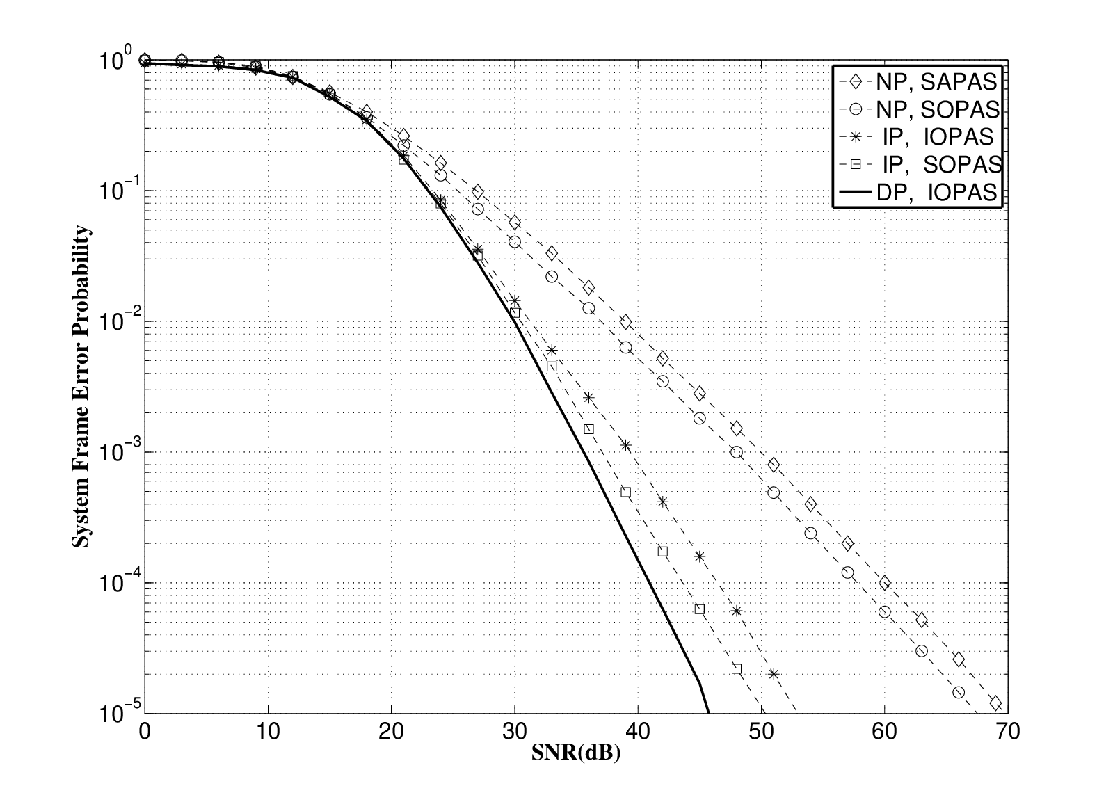
In our Monte-Carlo simulations, we choose 44-QAM modulation with 22 relays. Each frame has 44 symbols and each SFEP value is simulated by 10610^{6} i.i.di.i.d frames. Fig. 2 shows the SFEP under statistical CSI based power allocation schemes with different values of power allocation factor κ\kappa. We can see that when ρ\rho is large enough, systems reaches the lowest SFEP for 2​κ=1/32\kappa=1/3 and τ=2/3\tau=2/3, which validates Theorem 1.

Refer to caption
Fig. 2: SFEP in two-relay scenario with different power allocation schemes using 4-QAM modulation. Power allocation factor is the value of 2​κ2\kappa.
Refer to caption
Fig. 3: SFEP in two-relay scenario using 4-QAM modulation in 5 cases.

Fig. 3 compares the SFEP in six cases: 1) Statistical CSI based average power allocation scheme (SAPAS) without precoder (NP); 2) Statistical CSI based optimal power allocations scheme (SOPAS) without precoder; 3) Instantaneous s→rs\rightarrow{r} CSI based optimal power allocation scheme (IOPAS) with isolated precoders (IP); 4) SOPAS with IP; 5) IOPAS with DP. By SAPAS, both sources and relays consume the same power. We can see that power allocation scheme and precoders can distinctly improve the performance. Since IP with IOPAS can not achieve full diversity gain, it leads to worse performance even than that with SOPAS. However, DP with IOPAS achieves the best performance since it make the system achieve full diversity with larger Euclidian distance.

V Conclusion

In this letter, we propose two power allocation schemes and two precoders for 2−N−22-N-2 multicast systems with non-regenerative network coding. Although IP can help SOPAS achieve full diversity gain, it can not well help IOPAS. However, DP jointly with IOPAS can make the system not only achieve full diversity gain, but also outperform any other combinations of power allocation schemes and precoders in the term of SFEP.

References

  • [1] R. Ahlswede, N. Cai, S.-Y. R. Li and R. W. Yeung, “Network infomation flow,” IEEE Trans. Inf. Theory, vol. 46, no. 4, pp. 1204-1216, Jul. 2000.
  • [2] S. Zhang, S.-C. Liew, and P. P. Lam, “Hot topic: Physical-layer network coding,” in Proc. of 12th Annual International Conference on Mobile Computing and Networking (MobiCom), Los Angeles, CA, Sept. 23-26, 2006, pp. 358-365.
  • [3] T. Wang and G. B. Giannakis, “High-throughput cooperative communications with complex field network coding,” in Proc. of 41st Annual International Conference on Information Sciences and Systems (CISS), Baltimore, MD, Mar. 14-16, 2007, pp. 253-258.
  • [4] P. Popovski and H. Yomo, “Wireless network coding by amplify-and-forward for bi-directional traffic flows,” IEEE Communications Letters, vol. 11, no. 1, pp. 16-18, Jan. 2007.
  • [5] R. U. Nabar, H. Bo¨\ddot{\mathrm{o}}lcskei, and F. W. Kneubuhler, “Fading relay channels: Performance limits and space-time signal design,” IEEE J. Sel. Areas Commun., vol. 22, no. 6, pp. 1099-1109, Aug. 2004.
  • [6] Y. Xin, Z. Wang, and G. B. Giannakis, “Space-time diversity systems based on linear constellation precoding,” IEEE Trans. Wireless Commun., vol. 2, no. 2, pp. 294-309, Mar. 2003.
  • [7] Y. Ding, J.-K. Zhang, and K. M. Wong, “The amplify-and-forward half-duplex cooperative system: Pairwise error probability and precoder design,” IEEE Trans. Signal Process., vol. 55, no. 2, pp. 605-617, Feb. 2007.
  • [8] N. N Lebedev, Special functions and their applications, Englewood Cliffs, NJ: Prentice-Hall, 1965.
  • [9] David N. C. Tse and Stephen V. Hanly, “Multiaccess Fading Channels-Part I: Polymatroid Structure, Optimal Resource Allocation and Throughput Capacities,” IEEE Trans. Inf. Theory, vol. 44, no. 7, pp. 2796-2815, Nov. 1998.
  • [10] G. Caire, G. Taricco, and E. Biglieri, “Optimum power control over fading channels,” IEEE Trans. Inf. Theory, vol. 45, no. 5, pp. 1468-1489, Jul. 1998.