Old Problems, Classical Methods, New Solutions

Consider a standard heat equation in a one-sided domain with a moving boundary $b^{>}\left(t\right)$:

$$\begin{array}[]{c}\frac{\partial}{\partial t}E^{>}\left(t,x\right)=\frac{1}{2}\frac{\partial^{2}}{\partial x^{2}}E^{>}\left(t,x\right),\ \ \ b^{>}\left(t\right)\leq x<\infty,\\ \\ E^{>}\left(0,x\right)=\varepsilon^{>}\left(x\right),\ \ \ E^{>}\left(t,b^{>}\left(t\right)\right)=e^{>}\left(t\right),\ \ \ E\left(t,x\rightarrow\infty\right)\rightarrow 0.\end{array}$$

(1)

Without loss of generality, we can assume that $\varepsilon^{>}\left(x\right)=0$; the case of a nonzero initial condition can be solved by splitting:

$$\begin{array}[]{c}E^{>}=E\left(t,x\right)+F^{>}\left(t,x\right),\end{array}$$

$$\begin{array}[]{c}E\left(t,x\right)=\int_{b\left(t\right)}^{\infty}H\left(t,x-y\right)\varepsilon^{>}\left(y\right)dy,\end{array}$$

where $H\left(t,x\right)$ is the standard heat kernel,

$$\begin{array}[]{c}H\left(t,x\right)=\frac{e^{-\frac{x^{2}}{2t}}}{\sqrt{2\pi t}}.\end{array}$$

Thus, we can restrict ourselves to the case of zero initial condition:

$$\begin{array}[]{c}\frac{\partial}{\partial t}F^{>}\left(t,x\right)=\frac{1}{2}\frac{\partial^{2}}{\partial x^{2}}F^{>}\left(t,x\right),\ \ \ b^{>}\left(t\right)\leq x<\infty,\\ \\ F^{>}\left(0,x\right)=0,\ \ \ F^{>}\left(t,b^{>}\left(t\right)\right)=f^{>}\left(t\right),\ \ \ F\left(t,x\rightarrow\infty\right)\rightarrow 0,\end{array}$$

where

$$\begin{array}[]{c}f^{>}\left(t\right)=e^{>}\left(t\right)-E\left(t,b\left(t\right)\right).\end{array}$$

The MHP allows one to represent $F^{>}\left(t,x\right)$ in the form

$$\begin{array}[]{c}F^{>}\left(t,x\right)=\int_{0}^{t}\frac{\left(x-b^{>}\left(t^{\prime}\right)\right)\exp\left(-\frac{\left(x-b^{>}\left(t^{\prime}\right)\right)^{2}}{2\left(t-t^{\prime}\right)}\right)\nu^{>}\left(t^{\prime}\right)}{\sqrt{2\pi\left(t-t^{\prime}\right)^{3}}}dt^{\prime},\end{array}$$

(2)

where $\nu^{>}\left(t\right)$ solves the Volterra equation of the second kind:

$$\begin{array}[]{c}\nu^{>}\left(t^{\prime}\right)+\int_{0}^{t}\frac{\Theta^{>}\left(t,t^{\prime}\right)\Xi^{>}\left(t,t^{\prime}\right)\nu^{>}\left(t^{\prime}\right)}{\sqrt{2\pi\left(t-t^{\prime}\right)}}dt^{\prime}=f^{>}\left(t\right),\end{array}$$

(3)

and

$$\begin{array}[]{c}\ \Theta^{>}\left(t,t^{\prime}\right)=\frac{b^{>}\left(t\right)-b^{>}\left(t^{\prime}\right)}{\left(t-t^{\prime}\right)},\ \ \ \Xi^{>}\left(t,t^{\prime}\right)=e^{-\frac{\left(t-t^{\prime}\right)\Theta^{>2}\left(t,t^{\prime}\right)}{2}},\\ \\ \Theta^{>}\left(t,t\right)=\frac{db^{>}\left(t\right)}{dt},\ \ \ \Xi^{>}\left(t,t\right)=1.\end{array}$$

Similarly, the solution to the problem

$$\begin{array}[]{c}\frac{\partial}{\partial t}F^{<}\left(t,x\right)=\frac{1}{2}\frac{\partial^{2}}{\partial x^{2}}F^{<}\left(t,x\right),\ \ \infty<\ x\leq b^{<}\left(t\right),\\ \\ F^{<}\left(0,x\right)=0,\ \ \ F^{<}\left(t,x\rightarrow-\infty\right)\rightarrow 0,\ \ \ F^{<}\left(t,b\left(t\right)\right)=f^{<}\left(t\right),\end{array}$$

has the form

$$\begin{array}[]{c}F^{<}\left(t,x\right)=\int_{0}^{t}\frac{\left(x-b^{<}\left(t^{\prime}\right)\right)\exp\left(-\frac{\left(x-b^{<}\left(t^{\prime}\right)\right)^{2}}{2\left(t-t^{\prime}\right)}\right)\nu^{<}\left(t^{\prime}\right)}{\sqrt{2\pi\left(t-t^{\prime}\right)^{3}}}dt^{\prime},\end{array}$$

where

$$\begin{array}[]{c}-\nu^{<}\left(t^{\prime}\right)+\int_{0}^{t}\frac{\Theta^{<}\left(t,t^{\prime}\right)\Xi^{<}\left(t,t^{\prime}\right)\nu^{<}\left(t^{\prime}\right)}{\sqrt{2\pi\left(t-t^{\prime}\right)}}dt^{\prime}=f^{<}\left(t\right),\end{array}$$

Finally, the solution to the two-sided problem

$$\begin{array}[]{c}\frac{\partial}{\partial t}F^{><}\left(t,x\right)=\frac{1}{2}\frac{\partial^{2}}{\partial x^{2}}F^{><}\left(t,x\right),\ \ b^{>}\left(t\right)\leq\ x\leq b^{<}\left(t\right),\\ \\ F^{><}\left(0,x\right)=0,\ \ \ F^{><}\left(t,b^{<}\left(t\right)\right)=f^{<}\left(t\right),\ \ \ F^{><}\left(t,b^{>}\left(t\right)\right)=f^{>}\left(t\right),\end{array}$$

has the form

$$\begin{array}[]{c}F^{><}\left(t,x\right)=\int_{0}^{t}\frac{\left(x-b^{>}\left(t^{\prime}\right)\right)\exp\left(-\frac{\left(x-b^{>}\left(t^{\prime}\right)\right)^{2}}{2\left(t-t^{\prime}\right)}\right)\nu^{>}\left(t^{\prime}\right)}{\sqrt{2\pi\left(t-t^{\prime}\right)^{3}}}dt^{\prime}+\int_{0}^{t}\frac{\left(x-b^{<}\left(t^{\prime}\right)\right)\exp\left(-\frac{\left(x-b^{<}\left(t^{\prime}\right)\right)^{2}}{2\left(t-t^{\prime}\right)}\right)\nu^{<}\left(t^{\prime}\right)}{\sqrt{2\pi\left(t-t^{\prime}\right)^{3}}}dt^{\prime},\end{array}$$

$$\begin{array}[]{c}\nu^{>}\left(t^{\prime}\right)+\int_{0}^{t}\frac{\Theta^{>>}\left(t,t^{\prime}\right)\Xi^{>>}\left(t,t^{\prime}\right)\nu^{>}\left(t^{\prime}\right)}{\sqrt{2\pi\left(t-t^{\prime}\right)}}dt^{\prime}+\int_{0}^{t}\frac{\Theta^{><}\left(t,t^{\prime}\right)\Xi^{><}\left(t,t^{\prime}\right)\nu^{<}\left(t^{\prime}\right)}{\sqrt{2\pi\left(t-t^{\prime}\right)}}dt^{\prime}=f^{>}\left(t\right),\\ \\ -\nu^{<}\left(t^{\prime}\right)+\int_{0}^{t}\frac{\Theta^{<>}\left(t,t^{\prime}\right)\Xi^{<>}\left(t,t^{\prime}\right)\nu^{>}\left(t^{\prime}\right)}{\sqrt{2\pi\left(t-t^{\prime}\right)}}dt^{\prime}+\int_{0}^{t}\frac{\Theta^{<<}\left(t,t^{\prime}\right)\Xi^{<<}\left(t,t^{\prime}\right)\nu^{<}\left(t^{\prime}\right)}{\sqrt{2\pi\left(t-t^{\prime}\right)}}dt^{\prime}=f^{<}\left(t\right),\end{array}$$

where

$$\begin{array}[]{c}\Theta^{>>}\left(t,t^{\prime}\right)=\frac{b^{>}\left(t\right)-b^{>}\left(t^{\prime}\right)}{\left(t-t^{\prime}\right)},\ \ \ \Theta^{><}\left(t,t^{\prime}\right)=\frac{b^{>}\left(t\right)-b^{<}\left(t^{\prime}\right)}{\left(t-t^{\prime}\right)},\ \ \ \text{etc.}\end{array}$$

While Eqs (2), (3) provide an elegant solution to problem (1), in many instances we are interested in the behavior of this solution on the boundary itself. For instance, in numerous problems of mathematical finance, some of which are described below, what we need to know is the function

$$\begin{array}[]{c}g^{>}(t)=\frac{1}{2}\frac{\partial}{\partial x}F^{>}(t,b^{>}(t)),\end{array}$$

which represent the outflow of probability from the computational domain. This function can be calculated in two ways.

On the one hand, we can integrate the heat equation and get

$$\begin{array}[]{c}\frac{d}{dt}\mathop{\displaystyle\int}\limits_{b^{>}\left(t\right)}^{\infty}F^{>}\left(t,x\right)dx=\mathop{\displaystyle\int}\limits_{b^{>}\left(t\right)}^{\infty}\frac{\partial}{\partial t}F^{>}\left(t,x\right)dx=\frac{1}{2}\mathop{\displaystyle\int}\limits_{b^{>}\left(t\right)}^{\infty}\frac{\partial^{2}}{\partial x^{2}}F^{>}\left(t,x\right)dx=-\frac{1}{2}\frac{\partial}{\partial x}F^{>}(t,b^{>}(t))=-g^{>}\left(t\right).\end{array}$$

Eq. (2) yields

$$\begin{array}[]{c}\mathop{\displaystyle\int}\limits_{b^{>}\left(t\right)}^{\infty}F^{>}\left(t,x\right)dx=\int_{0}^{t}\frac{\Xi^{>}\left(t,t^{\prime}\right)\nu^{>}\left(t^{\prime}\right)}{\sqrt{2\pi\left(t-t^{\prime}\right)}}dt^{\prime},\end{array}$$

so that

$$\begin{array}[]{c}g^{>}\left(t\right)=-\frac{d}{dt}\int_{0}^{t}\frac{\Xi^{>}\left(t,t^{\prime}\right)\nu^{>}\left(t^{\prime}\right)}{\sqrt{2\pi\left(t-t^{\prime}\right)}}dt^{\prime}.\end{array}$$

(4)

On the other hand, a useful formula derived by the present author and his collaborators, see [35, 36, 37, 39], gives an alternative expression for $g^{>}\left(t\right)$:

$$\begin{array}[]{c}g^{>}\left(t\right)=-\left(\frac{1}{\sqrt{2\pi t}}+\frac{db^{>}\left(t\right)}{dt}\right)\nu^{>}\left(t\right)-\frac{1}{2}\int_{0}^{t}\frac{\left(\ \Phi^{>}\left(t,t^{\prime}\right)+\ \Theta^{>2}\left(t,t^{\prime}\right)\Xi^{>}\left(t,t^{\prime}\right)\nu^{>}\left(t^{\prime}\right)\right)}{\sqrt{2\pi\left(t-t^{\prime}\right)}}dt^{\prime},\end{array}$$

(5)

where

$$\begin{array}[]{c}\ \ \Phi^{>}\left(t,t^{\prime}\right)=\frac{\left(\nu^{>}\left(t\right)-\Xi^{>}\left(t,t^{\prime}\right)\nu^{>}\left(t^{\prime}\right)\right)}{\left(t-t^{\prime}\right)},\ \ \ \ \ \Phi^{>}\left(t,t\right)=\frac{d\nu^{>}\left(t\right)}{dt}+\frac{1}{2}\left(\frac{db^{>}\left(t\right)}{dt}\right)^{2}\nu^{>}\left(t\right).\end{array}$$

On the surface, Eqs (4), (5) look very different. However, a useful Lemma proven in [39], allows one to connect the two.

Lemma Let $\Psi\left(t,t^{\prime}\right)$ be a differentiable function, such that $\Psi\left(t,t\right)=1$. Then

$$\begin{array}[]{c}\frac{d}{dt}\int_{0}^{t}\frac{\Psi\left(t,t^{\prime}\right)\nu\left(t^{\prime}\right)}{\sqrt{2\pi\left(t-t^{\prime}\right)}}dt^{\prime}=\frac{\nu\left(t\right)}{\sqrt{2\pi t}}+\frac{1}{2}\int_{0}^{t}\frac{\nu\left(t\right)-\left(\Psi\left(t,t^{\prime}\right)-2\left(t-t^{\prime}\right)\Psi_{t}\left(t,t^{\prime}\right)\right)\nu\left(t^{\prime}\right)}{\sqrt{2\pi\left(t-t^{\prime}\right)^{3}}}dt^{\prime},\end{array}$$

Alternatively,

$$\begin{array}[]{c}\frac{d}{dt}\int_{0}^{t}\frac{\Psi\left(t,t^{\prime}\right)\nu\left(t^{\prime}\right)}{\sqrt{2\pi\left(t-t^{\prime}\right)}}dt^{\prime}=\int_{0}^{t}\frac{\frac{\partial}{\partial t^{\prime}}\left(\left(\Psi\left(t,t^{\prime}\right)-2\left(t-t^{\prime}\right)\Psi_{t}\left(t,t^{\prime}\right)\right)\nu\left(t^{\prime}\right)\right)}{\sqrt{2\pi\left(t-t^{\prime}\right)}}dt^{\prime}.\end{array}$$

We emphasize that Eq. (5) is easier to use than Eq. (4) in most situations because it does not involve differentiation. However, if the cumulative outflow $G^{>}\left(t\right)=\int_{0}^{t}g^{>}\left(t^{\prime}\right)dt^{\prime}$ is of interest, the latter equation can be more efficient, since it can be rewritten as follows:

$$\begin{array}[]{c}G^{>}\left(t\right)=-\int_{0}^{t}\frac{\Xi^{>}\left(t,t^{\prime}\right)\nu^{>}\left(t^{\prime}\right)}{\sqrt{2\pi\left(t-t^{\prime}\right)}}dt^{\prime}.\end{array}$$

We can calculate $g^{<}(t)$ and $g^{><}(t)$ by the same token. It is important to understand that both Eqs (5) and (4) can be used in the one-sided case, however, in the case when two boundaries are present, we can only use Eq. (5) because this equation allows calculating $g^{>}$ and $g^{<}$ individually while Eq. (4) calculates the difference $g^{>}-g^{<}$.

If the MHP were applicable only to standard Wiener process, it would be advantageous, if somewhat narrow in scope. Fortunately, it can be applied to a general diffusion satisfying the so-called Cherkasov’s condition, which guarantees that it can be transformed into the standard Wiener process. Such diffusions are studied in [9], [46], and [5]. The applications of Cherkasov’s condition in financial mathematics are discussed in [31], Section 4.2, and [34], Chapter 9.

Consider a diffusion governed by

$$\begin{array}[]{c}d\tilde{x}_{\tilde{t}}=\delta\left(\tilde{t},\tilde{x}_{\tilde{t}}\right)\,d\tilde{t}+\sigma\left(\tilde{t},\tilde{x}_{\tilde{t}}\right)\,dW_{\tilde{t}},\ \ \ \ \ \tilde{x}_{0}=\tilde{z},\end{array}$$

We wish to calculate boundary-related quantities, such as the distribution of the hitting time of a given time-dependent barrier $b\left(\tilde{t}\right)$:

$$\begin{array}[]{c}\tilde{s}=\inf\left\{\tilde{t}:\tilde{x}_{\tilde{t}}=\tilde{b}(\tilde{t})\right\},\ \ \ \ \ \tilde{z}\neq\tilde{b}(0).\end{array}$$

To this end, we introduce

$$\begin{array}[]{c}\beta\left(\tilde{t},\tilde{x}\right)=\sigma\left(\tilde{t},\tilde{x}\right)\int^{\tilde{x}}\frac{1}{\sigma\left(\tilde{t},y\right)}dy,\\ \\ \gamma\left(\tilde{t},\tilde{x}\right)=2\delta\left(\tilde{t},\tilde{x}\right)-\sigma\left(\tilde{t},\tilde{x}\right)\sigma_{\tilde{x}}\left(\tilde{t},\tilde{x}\right)-2\sigma\left(\tilde{t},\tilde{x}\right)\int^{\tilde{x}}\frac{\sigma_{\tilde{t}}\left(\tilde{t},y\right)}{\sigma^{2}\left(\tilde{t},y\right)}dy,\end{array}$$

where the lower limit of integration is chosen as convenient. Define

$$\begin{array}[]{c}P\left(\tilde{t},\tilde{x}\right)=\left|\begin{array}[]{cc}\beta\left(\tilde{t},\tilde{x}\right)&\gamma\left(\tilde{t},\tilde{x}\right)\\ \beta_{\tilde{x}}\left(\tilde{t},\tilde{x}\right)&\gamma_{\tilde{x}}\left(\tilde{t},\tilde{x}\right)\end{array}\right|,\\ \\ Q\left(\tilde{t},\tilde{x}\right)=\left|\begin{array}[]{cc}\sigma\left(\tilde{t},\tilde{x}\right)&\gamma\left(\tilde{t},\tilde{x}\right)\\ \sigma_{\tilde{x}}\left(\tilde{t},\tilde{x}\right)&\gamma_{\tilde{x}}\left(\tilde{t},\tilde{x}\right)\end{array}\right|,\\ \\ R\left(\tilde{t},\tilde{x}\right)=\left|\begin{array}[]{ccc}\sigma\left(\tilde{t},\tilde{x}\right)&\beta\left(\tilde{t},\tilde{x}\right)&\gamma\left(\tilde{t},\tilde{x}\right)\\ \sigma_{\tilde{x}}\left(\tilde{t},\tilde{x}\right)&\beta_{\tilde{x}}\left(\tilde{t},\tilde{x}\right)&\gamma_{\tilde{x}}\left(\tilde{t},\tilde{x}\right)\\ \sigma_{\tilde{x}\tilde{x}}\left(\tilde{t},\tilde{x}\right)&\beta_{\tilde{x}\tilde{x}}\left(\tilde{t},\tilde{x}\right)&\gamma_{\tilde{x}\tilde{x}}\left(\tilde{t},\tilde{x}\right)\end{array}\right|,\end{array}$$

and assume that Cherkasov’s condition is satisfied, so that

$$\begin{array}[]{c}R\left(\tilde{t},\tilde{x}\right)\equiv 0.\end{array}$$

Then we can transform $\tilde{x}$ into the standard Wiener process via the following mapping

$$\begin{array}[]{c}t=t(\tilde{t},\tilde{x})=\int_{0}^{\tilde{t}}\Phi^{2}(u,\tilde{x})du,\\ \\ x=x(\tilde{t},\tilde{x})=\Phi(\tilde{t},\tilde{x})\frac{\beta\left(\tilde{t},\tilde{x}\right)}{\sigma\left(\tilde{t},\tilde{x}\right)}+\frac{1}{2}\int_{0}^{\tilde{t}}\Phi(u,\tilde{x})\frac{P\left(u,\tilde{x}\right)}{\sigma\left(u,\tilde{x}\right)}du,\end{array}$$

where

$$\begin{array}[]{c}\Phi(\tilde{t},\tilde{x})=\exp\left[-\frac{1}{2}\int_{0}^{t}\frac{Q\left(u,\tilde{x}\right)}{\sigma\left(u,\tilde{x}\right)}du\right].\end{array}$$

In particular, the initial condition becomes

$$\begin{array}[]{c}z=\frac{\beta\left(0,\tilde{z}\right)}{\sigma\left(0,\tilde{z}\right)}.\end{array}$$

The corresponding transition probability density transforms as follows

$$\begin{array}[]{c}\tilde{p}(\tilde{t},\tilde{x};\tilde{z})=\left|\frac{\partial x(\tilde{t},\tilde{x})}{\partial\tilde{x}}\right|p(t,x;z).\end{array}$$

Moreover, the boundary transforms to

$$\begin{array}[]{c}\tilde{b}(\tilde{t})\rightarrow b(t)=\Phi(\tilde{t},\tilde{b}(\tilde{t}))\frac{\beta\left(\tilde{t},\tilde{b}(\tilde{t})\right)}{\sigma\left(\tilde{t},\tilde{b}(\tilde{t})\right)}+\frac{1}{2}\int^{\tilde{t}}\Phi(u,\tilde{b}(\tilde{t}))\frac{P\left(u,\tilde{b}(\tilde{t})\right)}{\sigma\left(u,\tilde{b}(\tilde{t})\right)}du.\end{array}$$

Since the MHP is specifically designed for dealing with curvilinear boundaries, we get a solvable problem. A powerful application of the above approach is demonstrated in Section 5, where the hitting time probability distribution for an Ornstein-Uhlenbeck process is studied.

There are numerous well-known approaches to solving Volterra equations; see, [30], among many others. We choose the most straightforward approach and show how to solve the following archetypal Volterra equation with weak singularity numerically:

$$\begin{array}[]{c}\nu(t)+\int_{0}^{t}\frac{K(t,t^{\prime})}{\sqrt{t-t^{\prime}}}\nu(t^{\prime})\,dt^{\prime}=f(t),\end{array}$$

where $K(t,t^{\prime})$ is a non-singular kernel. We write

$$\begin{array}[]{c}\int_{0}^{t}\frac{K(t,t^{\prime})\nu\left(t^{\prime}\right)}{\sqrt{t-t^{\prime}}}dt^{\prime}=-2\int_{0}^{t}K(t,t^{\prime})\nu\left(t^{\prime}\right)\,d\sqrt{t-t^{\prime}}.\end{array}$$

(6)

We wish to map this equation to a grid $0=t_{0}<t_{1}<\ldots<t_{N}=T$. To this end, we introduce the following notation:

$$\begin{array}[]{c}f_{k}=f(t_{k}),\ \ \ \nu_{k}=\nu\left(t_{k}\right),\ \ \ K_{k,l}=K(t_{k},t_{l}),\ \ \ \Delta_{k,l}=t_{k}-t_{l}.\end{array}$$

Then, the right hand side of Eq. (6) can be approximated by the trapezoidal rule as

$$\begin{array}[]{c}f_{k}=\nu_{k}+\sum_{l=1}^{k}\left(K_{k,l}\nu_{l}+K_{k,l-1}\nu_{l-1}\right)\Pi_{k,l}=0,\end{array}$$

(7)

where

$$\begin{array}[]{c}\Pi_{k,l}=\frac{\Delta_{l,l-1}}{\left(\sqrt{\Delta_{k,l-1}}+\sqrt{\Delta_{k,l}}\right)},\end{array}$$

so that

$$\begin{array}[]{c}\nu_{k}=\frac{\left(f_{k}-K_{k,k-1}\nu_{k-1}-\sum_{l=1}^{k-1}\left(K_{k,l}\nu_{l}+K_{k,l-1}\nu_{l-1}\right)\Pi_{k,l}\right)}{\left(1+K_{k,k}\sqrt{\Delta_{k,k-1}}\right)}.\end{array}$$

(8)

Thus, $\nu_{k}$ can be found by induction starting with $\nu_{0}=f_{0}$.

Eq. (8) is the blueprint for all the subsequent numerical calculations.

The original, and straightforward, structural default model was introduced by Merton, [41], who assumed that default could happen only at debt maturity. His model was extended by Black and Cox, [4], who considered the default, which can happen at any time by introducing flat default boundary representing debt covenants. Numerous authors expanded their model including [19, 18, 3], who considered curvilinear boundary whose shape can be calibrated to the market default probability. One of the major unsolved issues with the above model was articulated by Hyer et al., [19], who pointed out that, unless the shape of the default boundary is very carefully chosen, the probability of short-term default is too low. This issue was addressed by several authors, including [13, 17, 32], who proposed to introduce jump and or uncertainty to increase this probability. We show below that it is possible to calibrate the default boundary in such a way that constant default intensity can be matched. We emphasize that the direct problem - calculating the default probability given the boundary - is linear (albeit relatively involved), while the inverse problem - finding the boundary given the default probability - is nonlinear (and hence even more involved). Additional details are given in [37].

We wish to find the boundary for a structural default model corresponding to a constant default intensity $\eta$. We denote the corresponding default probability by

$$\begin{array}[]{c}\pi\left(t\right)=1-e^{-\eta t}.\end{array}$$

The introduce time $\tau$, such that default is impossible for $t<\tau$. Thus the default boundary starts at $t=\tau$. The idea is to calculate the corresponding boundary $b\left(t;\tau,\eta\right)$, provided it exists, and then let $\tau\rightarrow 0$.

It is clear that at time $t=\tau-0$, the transition probability is

$$\begin{array}[]{c}p(\tau,x)=H\left(\tau,x\right),\end{array}$$

where $H$ is the heat kernel:

$$\begin{array}[]{c}H\left(\tau,x\right)=\frac{e^{-\frac{x^{2}}{2\tau}}}{\sqrt{2\pi\tau}}.\end{array}$$

At time $t=\tau$, the first possibility of default occurs. For $t>\tau$ the transition probability satisfies the following Fokker–Planck problem

$$\begin{array}[]{c}\frac{\partial}{\partial t}p(t,x)=\frac{1}{2}\frac{\partial^{2}}{\partial x^{2}}p(t,x),\ \ \ \ \ b\left(t\right)\leq x<\infty,\\ \\ p\left(\tau,x\right)=H\left(\tau,x\right),\ \ \ p\left(t,b\left(t\right)\right)=0,\ \ \ p\left(t,x\rightarrow\infty\right)\rightarrow 0.\end{array}$$

The default probability density $g(t)$ is given by

$$\begin{array}[]{c}g(t)=\frac{1}{2}\frac{\partial}{\partial x}p(t,b(t)).\end{array}$$

Alternatively,

$$\begin{array}[]{c}\pi(t)=1-\int_{b(t)}^{\infty}p(t,x)\,dx,\ \ \ g(t)=\frac{d\pi\left(t\right)}{dt}.\end{array}$$

We split $p$ as follows

$$p(t,x)=q(t,x)+r(t,x),$$

where

$$\begin{array}[]{c}\frac{\partial}{\partial t}q(t,x)=\frac{1}{2}\frac{\partial^{2}}{\partial x^{2}}q(t,x),\ \ \ \ \ -\infty<x<\infty,\\ \\ q\left(\tau,x\right)=H\left(\tau,x\right)\Theta\left(x-b\left(\tau\right)\right),\ \ \ q\left(t,x\rightarrow-\infty\right)\rightarrow 0,\ \ \ q\left(t,x\rightarrow\infty\right)\rightarrow 0,\end{array}$$

(9)

$$\begin{array}[]{c}\frac{\partial}{\partial t}r(t,x)=\frac{1}{2}\frac{\partial^{2}}{\partial x^{2}}r(t,x),\ \ \ \ \ b\left(t\right)\leq x<\infty,\\ \\ r\left(\tau,x\right)=0,\ \ \ r\left(t,b\left(t\right)\right)=-q\left(t,b\left(t\right)\right),\ \ \ r\left(t,x\rightarrow\infty\right)\rightarrow 0.\end{array}$$

and $\Theta\left(x\right)$ is the Heaviside function. Solving Eq. (9) as a convolution of heat kernel with the initial condition, we get

$$\begin{array}[]{c}q(t,x)=\frac{e^{-\frac{x^{2}}{2t}}}{\sqrt{2\pi t}}N\left(\frac{\frac{ux}{t}-b\left(\tau\right)}{\sqrt{u}}\right),\end{array}$$

where $u=(t-\tau)\tau/t$, see [37]. Thus

$$\begin{array}[]{c}g\left(t\right)=\frac{1}{2}\frac{\partial}{\partial x}r\left(t,b\left(t\right)\right)-\frac{H\left(t,b\left(t\right)\right)}{2t}\left(b\left(t\right)N\left(\frac{\frac{ub\left(t\right)}{t}-b\left(\tau\right)}{\sqrt{u}}\right)-uH\left(u,\frac{ub\left(t\right)}{t}-b\left(\tau\right)\right)\right).\end{array}$$

Accordingly, in view the discussion in Section 2.2, we need to solve the following system of integral equations:

$$\begin{array}[]{c}\nu\left(t\right)+\int_{\tau}^{t}\frac{\Theta\left(t,t^{\prime}\right)\Xi\left(t,t^{\prime}\right)\nu\left(t^{\prime}\right)}{\sqrt{2\pi\left(t-t^{\prime}\right)}}dt^{\prime}+H\left(t,b\left(t\right)\right)N\left(\frac{ub\left(t\right)-tb\left(\tau\right)}{t\sqrt{u}}\right)=0,\\ \\ \eta e^{-\eta t}+\left(\frac{1}{\sqrt{2\pi t}}+\frac{db\left(t\right)}{dt}\right)\nu\left(t\right)+\frac{1}{2}\int_{\tau}^{t}\frac{\Phi\left(t,t^{\prime}\right)+\Theta^{2}\left(t,t^{\prime}\right)\Xi\left(t,t^{\prime}\right)\nu\left(t^{\prime}\right)}{\sqrt{2\pi\left(t-t^{\prime}\right)}}dt^{\prime}\\ \\ +\frac{H\left(t,b\left(t\right)\right)}{2t}\left(b\left(t\right)N\left(\frac{\frac{ub\left(t\right)}{t}-b\left(\tau\right)}{\sqrt{u}}\right)-uH\left(u,\frac{ub\left(t\right)}{t}-b\left(\tau\right)\right)\right)=0.\end{array}$$

(10)

Alternatively, we can rewrite Eqs (10) in integrated form

$$\begin{array}[]{c}\nu\left(t\right)+\int_{\tau}^{t}\frac{\Theta\left(t,t^{\prime}\right)\Xi\left(t,t^{\prime}\right)\nu\left(t^{\prime}\right)}{\sqrt{2\pi\left(t-t^{\prime}\right)}}dt^{\prime}+H\left(t,b\left(t\right)\right)N\left(\frac{ub\left(t\right)-tb\left(\tau\right)}{t\sqrt{u}}\right)=0,\\ \\ 1-e^{-\eta t}+\int_{\tau}^{t}\frac{\Xi\left(t,t^{\prime}\right)\nu\left(t^{\prime}\right)}{\sqrt{2\pi\left(t-t^{\prime}\right)}}dt^{\prime}-N\left(\frac{b\left(t\right)}{\sqrt{t}}\right)-N\left(\frac{\sqrt{t}b\left(\tau\right)}{\sqrt{u\left(u+t\right)}}\right)+BVN\left(\frac{\sqrt{t}b\left(\tau\right)}{\sqrt{u\left(u+t\right)}},\frac{b\left(t\right)}{\sqrt{t}};\sqrt{\frac{u}{u+t}}\right)=0,\end{array}$$

(11)

where $BVN\left(.,.;.\right)$ is the bivariate normal distribution.

We postpone the discussion of the corresponding numerics until the next Section, where a more general case is considered.

Recall that the default probability has the form

$$\begin{array}[]{c}\pi(t)=1-e^{-\eta t}.\end{array}$$

The barrier has to start at $\tau=\hat{\tau}$, $\hat{\tau}\rightarrow 0$, and there should be no barrier before that. We wish to find $b\left(\hat{\tau}\right)$ such that

$$\begin{array}[]{c}\pi\left(\hat{\tau}\right)=1-\int_{b\left(\hat{\tau}\right)}^{\infty}\frac{\exp\left(-\frac{x^{2}}{2\hat{\tau}}\right)}{\sqrt{2\pi\hat{\tau}}}dx=1-N\left(-\frac{b\left(\hat{\tau}\right)}{\sqrt{\hat{\tau}}}\right)=1-e^{-\eta\hat{\tau}}.\end{array}$$

Thus,

$$\begin{array}[]{c}N\left(-\frac{b\left(\hat{\tau}\right)}{\sqrt{\hat{\tau}}}\right)=e^{-\eta\hat{\tau}},\end{array}$$

and

$$\begin{array}[]{c}b\left(\hat{\tau}\right)=-\sqrt{\hat{\tau}}N^{-1}\left(e^{-\eta\hat{\tau}}\right).\end{array}$$

Now,

$$\begin{array}[]{c}N^{-1}\left(y\right)\underset{y\rightarrow 1}{\sim}\sqrt{2f\left(\eta\right)},\end{array}$$

where

$$\begin{array}[]{c}\eta=-\ln\left(2\sqrt{\pi}\left(1-y\right)\right),\ \ \ f\left(\eta\right)=\eta-\frac{\ln\eta}{2}+\frac{\ln\eta-2}{4\eta}+\frac{\left(\ln\eta\right)^{2}-6\ln\eta+14}{16\eta^{2}},\end{array}$$

so that

$$\begin{array}[]{c}b\left(\hat{\tau}\right)=-\sqrt{2\hat{\tau}f\left(-\ln\left(2\sqrt{\pi}\left(1-e^{-\eta\hat{\tau}}\right)\right)\right)}\approx-\sqrt{2\hat{\tau}\ln\left(\frac{1}{2\sqrt{\pi}\eta\hat{\tau}}\right)}.\end{array}$$

Default boundaries calibrated to several representative values of $\eta$ are shown in Figure 1.

Figure 1 near here.

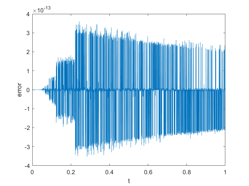
We show that solutions of Eqs (10) and Eqs (11) coincide modulo numerical error in Figure 2.

Figure 2 near here.

Conjecture For a given time interval $I^{\left(T\right)}=\left[0,T\right]$, there exists a parameter interval $I^{\left(\eta\right)}\left(T\right)=\left[0,\eta^{\ast}\left(T\right)\right]$, such that for any $\eta\in I^{\left(\eta\right)}\left(T\right)$, the default boundary $b\left(t\right)$ can be calibrated to the default intensity $\eta$. We can construct the corresponding boundary as follows:

$$\begin{array}[]{c}b\left(t;\eta\right)=\lim_{\tau\rightarrow 0}b\left(t;\tau,\eta\right),\ \ \ 0<t\leq T,\end{array}$$

where $b\left(t;\tau,\eta\right)$ is found by solving either Eqs (10) or Eqs (11).

We illustrate our conjecture in Figure 3.

Figure 3 near here.

No bank is an island - they operate as a group. Tangible links between banks manifest themselves via interbank loans; intangible links are manifold - overall sentiment, ease of doing business, and others. Hence, to build a meaningful structural default model for a bank, one needs to take into account this bank’s interactions with all the banks whom it lends to or borrows from. Eisenberg and Noe developed a Merton-like model of the bank default (default can happen only at maturity) in the seminal paper [12]. The present author extended the Eisenberg-Noe model to the Black-Cox setting (default can happen at any time before maturity provided that debt covenants are violated); see [33]. Lipton’s work was subsequently generalized in [21, 22]. Recently, several authors considered the interconnected banking system in the mean-field framework and studied a representative bank, see [16, 20, 25, 42, 43] among many others. In this section, we also use the mean-field approach. Additional details are given in [39].

We follow [33] and assume that the dynamics of bank $i$’s total external assets is governed by

$$\begin{array}[]{c}\frac{dA_{t}^{i}}{A_{t}^{i}}=\mu_{i}\,dt+\sigma_{i}\,dW_{t}^{i},\end{array}$$

where $W^{i}$ are independent standard Brownian motions for $1\leq i\leq n$, and the liabilities, both external $L_{i}$ and mutual $L_{ij}$, are constant.

Bank $i$ is assumed to default when its assets fall below a certain threshold determined by its liabilities, namely at time $\tau_{i}=\inf\{t:A_{t}^{i}\leq\Lambda_{t}^{i}\}$, where $\Lambda^{i}$ is a default boundary which we now work out. At time $t=0$,

$$\begin{array}[]{c}\Lambda_{0}^{i}=R_{i}\left(L_{i}+\sum_{j\neq i}L_{ij}\right)-\sum_{j\neq i}L_{ji},\end{array}$$

where $R_{i}$ is the recovery rate of bank $i$. If bank $k$ defaults at time $t$, the default boundary of bank $i$ jumps by $\Delta\Lambda_{t}^{i}=(1-R_{i}R_{k})L_{ki}.$

References

• [1] Alili, L., Patie, P. and Pedersen, J.L. (2005). Representations of the first hitting time density of an Ornstein–Uhlenbeck process. Stoch. Models, 21(4), 967–980.
• [2] Andersen, L. and Lipton, A. (2013). Asymptotics for exponential L´evy processes and their volatility smile: survey and new results. International Journal of Theoretical and Applied Finance, 16 (1) 1350001 (98 pages).
• [3] Avellaneda, M. and Zhu, J. (2001). Distance to default. Risk, 14(12), 125–129.
• [4] Black, F. and and Cox, J.C. (1976). Valuing corporate securities: Some effects of bond indenture provisions, J. Finance 31(2), 351–367.
• [5] Bluman, G.W. (1980). On the transformation of diffusion processes into the Wiener process. SIAM. J. Appl. Math., 39(2), 238–247.
• [6] Borodin, A.N. and Salminen, P. (2012). Handbook of Brownian Motion: Facts and Formulae, (Birkhäuser, Basel).
• [7] Breiman, L. (1967). First exit times from a square root boundary. In Fifth Berkeley Symposium, Vol. 2, pp. 9–16 (Berkeley).
• [8] Carrillo, J., Gonz´alez, M., Gualdani, M. and Schonbek, M. (2013). Classical solutions for a nonlinear Fokker-Planck equation arising in computational neuroscience, Comm. Partial Differential Equations 38(3), 385–409.
• [9] Cherkasov, I.D. (1957). On the transformation of the diffusion process to a Wiener process. Theor. Probab. Appl., 2(3), 373–377.
• [10] Delarue, F., Nadtochiy, S. and Shkolnikov, M. (2017). Global solutions to the supercooled Stefan problem with blow-ups: regularity and uniqueness. arXiv preprint.
• [11] Einstein, A. (1905). Über die von der molekularkinetischen theorie der wärme geforderte bewegung von in ruhenden flüssigkeiten suspendierten teilchen. Ann. Phys., 322(8), 549–560.
• [12] Eisenberg, L. and Noe, T. H. (2001). Systemic risk in financial systems. Management Science, 47(2), 236–249.
• [13] Finkelstein V and Lardy, J. P. (2001) Assessing default probabilities from equity markets: simple closed-form solution. Presented at the ICBI Global Derivatives Conference, Juan les Pins.
• [14] Fortet, R. (1943) Les fonctions altatoires du type de markoff associees a certaines equations linlaires aux dfrivees partielles du type parabolique. J. Math. Pures Appl., 22, 177–243.
• [15] Göing-Jaeschke, A. and Yor, M. (2003). A clarification note about hitting times densities for Ornstein–Uhlenbeck processes. Finance Stoch., 7(3), 413–415.
• [16] Hambly, B., Ledger, S., and Sojmark, A. (2018). A McKean–Vlasov equation with positive feedback and blow-ups. arXiv preprint.
• [17] Hilberink. B., and Rogers, L. (2002) Optimal capital structure and endogenous default Finance and Stochastics 6, 237–263.
• [18] Hull, J., and White, A. (2001). Valuing credit default swaps, II. Journal of Derivatives 8(3), 12–22.
• [19] Hyer, T., Lipton, A., Pugachevsky, D., and Qui, S. (1998). A hidden-variable model for risky bonds. Bankers Trust working paper.
• [20] Ichiba, T., Ludkovski, M., and Sarantsev, A. (2018). Dynamic contagion in a banking system with births and defaults. arXiv preprint.
• [21] Itkin, A. and Lipton, A. (2015). Efficient solution of structural default models with correlated jumps and mutual obligations. International Journal of Computer Mathematics, 92(12), 2380–2405.
• [22] Itkin, A. and Lipton, A. (2017). Structural default model with mutual obligations. Review of Derivatives Research, 20,15–46.
• [23] Kamenomostskaja, S. L. (1961). On Stefan’s problem, Mat. Sb. (N.S.) 53 (95), 489–514.
• [24] Kartashov, E. (2001). Analytical Methods in the Theory of Heat Conduction of Solids. Vysshaya Shkola, Moscow 706.
• [25] Kaushansky, V. and Reisinger, C. (2018). Simulation of particle systems interacting through hitting times. arXiv preprint.
• [26] Leblanc, B. and Scaillet, O. (1998). Path dependent options on yields in the affine term structure model. Finance Stoch., 2(4), 349–367.
• [27] Leblanc, B., Renault, O. and Scaillet, O. (2000) A correction note on the first passage time of an Ornstein-Uhlenbeck process to a boundary. Finance Stoch., 4(1), 109–111.
• [28] Lewis, T. J. and Rinzel, J. (2003). Dynamics of spiking neurons connected by both inhibitory and electrical coupling, J. Comput. Neurosci. 14(3), 283–309.
• [29] Linetsky, V. (2004) Computing hitting time densities for CIR and OU diffusions: Applications to mean-reverting models. J. Comput. Finance, 7, 1–22.
• [30] Linz, P. (1985) Analytical and Numerical Methods for Volterra Equations (SIAM, Philadelphia, PA).
• [31] Lipton, A. (2001). Mathematical Methods for Foreign Exchange: A Financial Engineer’s Approach. World Scientific, Singapore.
• [32] Lipton, A. (2002). Assets with Jumps. Risk 15 (9), 149–153.
• [33] Lipton, A. (2016). Modern monetary circuit theory, stability of interconnected banking network, and balance sheet optimization for individual banks. International Journal of Theoretical and Applied Finance, 19(6).
• [34] Lipton, A. (2018) Financial Engineering: Selected Works of Alexander Lipton. World Scientific, Singapore.
• [35] Lipton, A. and Kaushansky, V. (2018). On the first hitting time density of an Ornstein-Uhlenbeck process. arXiv preprint.
• [36] Lipton, A. and Kaushansky, V. (2020). On the first hitting time density for a reducible diffusion process. Quantitative Finance. DOI: 10.1080/14697688.2020.1713394
• [37] Lipton, A. and Kaushansky, V. (2020). Physics and Derivatives: On Three Important Problems in Mathematical Finance. The Journal of Derivatives.
• [38] Lipton, A. and Lopez De Prado, M. (2020). A closed-form solution for optimal mean-reverting trading strategies. https://papers.ssrn.com/sol3/papers.cfm?abstract_id=3534445.
• [39] Lipton, A., Kaushansky, V. and Reisinger, C. (2019).Semi-analytical solution of a McKean–Vlasov equation with feedback through hitting a boundary. European Journal of Applied Mathematics. doi:10.1017/S0956792519000342.
• [40] Lopez De Prado, M. (2018). Advances in financial machine learning. John Wiley Sons, Hoboken, NJ.
• [41] Merton, R. (1974). On the pricing of corporate debt: the risk structure of interest rates. Journal of Finance 29, 449–470.
• [42] Nadtochiy, S. and Shkolnikov, M. (2017). Particle systems with singular interaction through hitting times: application in systemic risk modeling. arXiv preprint.
• [43] Nadtochiy, S. and Shkolnikov, M. (2018). Mean field systems on networks, with singular interaction through hitting times. arXiv preprint.
• [44] Ostojic, S., Brunel, N. and Hakim, V. (2009). Synchronization properties of networks of electrically coupled neurons in the presence of noise and heterogeneities, J. Comput. Neurosci. 26, no. 3, 369–392.
• [45] Polyanin, A.D. and Manzhirov, A.V. (1998). Handbook of Integral Equations, CRC Press, Boca Raton, FL.
• [46] Ricciardi, L.M. (1976). On the transformation of diffusion processes into the Wiener process. J. Math. Anal. Appl., 54(1), 185–199.
• [47] Ricciardi, L.M. and Sato, S. (1988). First-passage-time density and moments of the Ornstein–Uhlenbeck process. J. Appl. Probab., 25(1), 43–57.
• [48] Rubinstein, L. (1971). The Stefan Problem. Vol. 27 of Translations of Mathematical Monographs. American Mathematical Society, Providence, RI.
• [49] Von Smoluchowski, M. (1906). Zur kinetischen theorie der brownschen molekularbewegung und der suspensionen. Ann. Phys., 326(14), 756–780.
• [50] Tikhonov, A. N., and Samarskii, A. A.. (1963). Equations of Mathematical Physics. Dover Publications, New York. English translation.
• [51] Watson, N. A. (2012). Introduction to Heat Potential Theory. Number 182 in Mathematical Surveys and Monographs. American Mathematical Society, Providence, RI.
Refer to caption
(a)
(b)
Figure 1: In Figures (a)-(b), we show the default boundaries for several representative values of the default intensity η\eta. We choose τ=0.01\tau=0.01. In Figure (a), we choose 0.01<t<10.00.01<t<10.0 to capture their overall behavior; In Figure (b), we choose 0.01<t<0.10.01<t<0.1 so that small features can be shown.
Figure 2: In this figure, we choose the default intensity η=0.09\eta=0.09 and show that boundaries calculated by solving Eqs (10) and Eqs (11) coincide modulo numerical errors.
(c)
Figure 3: In this figure, we choose the default intensity η=0.05\eta=0.05 and illustrate our main conjecture numerically by constructing three boundaries corresponding to τ=0.01\tau=0.01, 0.0010.001, and 0.00050.0005, respectively. It is clear that after a short initial period, these boundaries begin overlapping.
Figure 4: In this figure, we demonstrate the loss probability for the initial position z=0.5z=0.5 and several representative values of α\alpha, which characterizes the strength of interbank interactions.
Figure 5: In Figures (a)-(b), we choose z=0.5,z=0.5, α=0,\alpha=0, and we show μ⁡(t)\mu\left(t\right) and ν⁡(t)\nu\left(t\right) calculated numerically and analytically. In Figure (c), we choose z=0.5,z=0.5, α=0.6,\alpha=0.6, and we show the error generated by the Newton-Raphson method.
(d)
(e)
(f)
Figure 6: In Figures (a)-(f) we show the probability denstity function p⁡(t,x−z,z)p\left(t,x-z;z\right). We shift the domain down by −z-z in order to make comparison with the structural default model considered in Section 3 more transparent. In Figures (a) and (b) we show analytical and numerical results for α=0\alpha=0. In Figures (c)-(f) we show numerical results for α=0.2\alpha=0.2, 0.40.4, 0.60.6, 0.80.8, respectively.
Figure 7: In Figures (a)-(f), we show the pdf and cdf for the hitting time probability distribution. In Figures (a), (b) z=2z=2, b⁡(t)=0b\left(t\right)=0, so that both numerical and analytical expressions are available. These expressions are in perfect agreement. In Figures (c), (d) z=2z=2, b⁡(t)=0b\left(t\right)=0 and b⁡(t)=0.2​sin⁡(10.0​t)b\left(t\right)=0.2\sin\left(10.0t\right). In Figures (e), (f) z=2z=2, b⁡(t)=1.0b\left(t\right)=1.0 and b⁡(t)=1.0+0.2​sin⁡(10.0​t)b\left(t\right)=1.0+0.2\sin\left(10.0t\right). Variations in the pdf caused by the barrier undulations are astonishingly profound.
Figure 8: In this figure, we show the solid-liquid boundaries b(t) for several representative values of α\alpha.
Figure 9: In Figures (a)-(b) we show the stationary distribution p⁡(x)p\left(x\right) and its derivative d​p​(x)/d​xdp\left(x\right)/dx for the following parameter values: X0=−1X_{0}=-1, m0=0.5m_{0}=0.5, m1=0.1m_{1}=0.1. The corresponding value of λ\lambda, which is computed as part of the solution, is 1.40021.4002 .