Improved Approximations of Hedges’ g*

Xiaohuan Xue Address: Department of Mathematics and Statistics, Wake Forest University, Winston-Salem, North Carolina 27109 Current address: Department of Psychology, University of California, Los Angeles, California 90095 Email address: xhxue@g.ucla.edu

Abstract.

Hedges’ unbiased estimator g* has been broadly used in statistics. We propose a sequence of polynomials to better approximate the multiplicative correction factor of g* by incorporating analytic estimations to the ratio of gamma functions.

Key words and phrases:

Gamma function, polynomial approximation, standardized mean difference

2010 Mathematics Subject Classification

Primary 41A10; Secondary 33B15, 41A60, 62H12, 62P10

1. Introduction

Hedges proposed the widely used unbiased estimator, $g*$ , of standardized mean differences [1, 2, 3]. Suppose group $i$ with sample size $n_{i}$ is $y_{i1},\cdots,y_{in_{i}}$ , and group $j$ with sample size $n_{j}$ are $y_{j1},\cdots,y_{in_{j}}$ , and we assume the samples in two groups are normally distributed with the same variance, that is,

(1.1)

y_{i1},\cdots,y_{in_{i}}\sim N(\mu_{i},\sigma^{2})

(1.2)

y_{j1},\cdots,y_{jn_{j}}\sim N(\mu_{j},\sigma^{2})

Hedges’ $g*$ is given by the sample mean difference divided by a multiple of the pooled sample standard deviation as following

(1.3)

g*=J(n_{i}+n_{j}-2)\cdot\frac{\overline{y}_{j}-\overline{y}_{i}}{s_{p}}

where

(1.4)

J(m)=\frac{\Gamma(\frac{m}{2})}{\sqrt{\frac{m}{2}}\Gamma(\frac{m-1}{2})}

and $s_{p}$ is the pooled sample standard deviation

(1.5)

s_{p}=\sqrt{\frac{(n_{j}-1)s_{j}^{2}+(n_{i}-1)s_{i}^{2}}{n_{j}+n_{i}-2}}

The multiplicative correction term $J(\cdot)$ in Hedges’ $g*$ is not easy to calculate in practice, and one commonly used approximation is given by Hedges [1, 2]

(1.6)

J(m)=\frac{\Gamma(\frac{m}{2})}{\sqrt{\frac{m}{2}}\Gamma(\frac{m-1}{2})}\approx 1-\frac{3}{4m-1}

and let us denote Hedges’ estimation as $H(m)$ :

(1.7)

H(m)=1-\frac{3}{4m-1}

We now propose a sequence of polynomials to give more accurate approximations of $J(\cdot)$ and thus improve the accuracy of Hedges’ $g*$ .

2. Wallis Ratio and Approximation of Hedge’s Estimator

The Wallis ratio [4, 5, 6] is defined by

(2.1)

\frac{\Gamma(x+1)}{\Gamma(x+\frac{1}{2})}

and we can see

(2.2)

\sqrt{\frac{m}{2}}J(m)=\frac{\Gamma(\frac{m}{2})}{\Gamma(\frac{m-1}{2})}

is a special case of Wallis ratio when $x=\frac{m}{2}-1$ . Thus the approximations of Wallis ration as a result of properties of gamma function can be applied to estimating $J(\cdot)$ .

For Wallis ratio, there are Mortici’s approximations [5, 6, 7]

(2.3)

\frac{\Gamma(x+1)}{\Gamma(x+\frac{1}{2})}\approx\sqrt{x+\frac{1}{4}}

(2.4)

\frac{\Gamma(x+1)}{\Gamma(x+\frac{1}{2})}\approx\sqrt[4]{x^{2}+\frac{1}{2}x+\frac{1}{8}}

(2.5)

\frac{\Gamma(x+1)}{\Gamma(x+\frac{1}{2})}\approx\sqrt[6]{x^{3}+\frac{3}{4}x^{2}+\frac{9}{32}x+\frac{5}{128}}

(2.6)

\frac{\Gamma(x+1)}{\Gamma(x+\frac{1}{2})}\approx\sqrt[8]{x^{4}+x^{3}+\frac{1}{2}x^{2}+\frac{1}{8}x}

(2.7)

\frac{\Gamma(x+1)}{\Gamma(x+\frac{1}{2})}\approx\sqrt[10]{x^{5}+\frac{5}{4}x^{4}+\frac{25}{32}x^{3}+\frac{35}{128}x^{2}+\frac{75}{2048}x+\frac{3}{8192}}

(2.8)

\frac{\Gamma(x+1)}{\Gamma(x+\frac{1}{2})}\approx\sqrt[12]{x^{6}+\frac{3}{2}x^{5}+\frac{9}{8}x^{4}+\frac{1}{2}x^{3}+\frac{15}{128}x^{2}+\frac{3}{256}x+\frac{11}{1024}}

By letting $x=\frac{m}{2}-1$ , we can have an approximation of $J(m)$

(2.9)

J(m)\approx P_{1}(m)=\sqrt{1-\frac{3}{2m}}

(2.10)

\begin{split}J(m)\approx P_{2}(m)&=\sqrt{\frac{2}{m}}\sqrt[4]{(\frac{m}{2}-1)^{2}+\frac{1}{2}(\frac{m}{2}-1)+\frac{1}{8}}\\ &=\sqrt[4]{1-\frac{3}{m}+\frac{5}{2m^{2}}}\end{split}

(2.11)

\begin{split}J(m)\approx P_{3}(m)&=\sqrt{\frac{2}{m}}\sqrt[6]{(\frac{m}{2}-1)^{3}+\frac{3}{4}(\frac{m}{2}-1)^{2}+\frac{9}{32}(\frac{m}{2}-1)+\frac{5}{128}}\\ &=\sqrt[6]{1-\frac{9}{2m}+\frac{57}{8m^{2}}-\frac{63}{16m^{3}}}\end{split}

(2.12)

\begin{split}J(m)\approx P_{4}(m)&=\sqrt{\frac{2}{m}}\sqrt[8]{(\frac{m}{2}-1)^{4}+(\frac{m}{2}-1)^{3}+\frac{1}{2}(\frac{m}{2}-1)^{2}+\frac{1}{8}(\frac{m}{2}-1)}\\ &=\sqrt[8]{1-\frac{6}{m}+\frac{14}{m^{2}}-\frac{15}{m^{3}}+\frac{6}{m^{4}}}\end{split}

(2.13)

\begin{split}J(m)&\approx P_{5}(m)\\ &=\sqrt{\frac{2}{m}}\sqrt[10]{(\frac{m}{2}-1)^{5}+\frac{5}{4}(\frac{m}{2}-1)^{4}+\frac{25}{32}(\frac{m}{2}-1)^{3}+\frac{35}{128}(\frac{m}{2}-1)^{2}+\frac{75}{2048}(\frac{m}{2}-1)+\frac{3}{8192}}\\ &=\sqrt[10]{1-\frac{15}{2m}+\frac{185}{8m^{2}}-\frac{585}{16m^{3}}+\frac{3755}{128m^{4}}-\frac{2409}{256m^{5}}}\end{split}

(2.14)

J(m)\approx P_{6}(m)=\sqrt[12]{1-\frac{9}{m}+\frac{69}{2m^{2}}-\frac{72}{m^{3}}+\frac{687}{8m^{4}}-\frac{441}{8m^{5}}+\frac{247}{16m^{6}}}

3. Accuracy of different approximations

In this section, we compare the accuracy of all the given approximations by measuring the absolute values of their errors to the real value with a broad range of $m$ . For convenience, we introduce the notations for the absolute errors

(3.1)

\delta_{0}(m)=|H(m)-J(m)|

(3.2)

\delta_{i}(m)=|P_{i}(m)-J(m)|;i=1,\cdots,6.

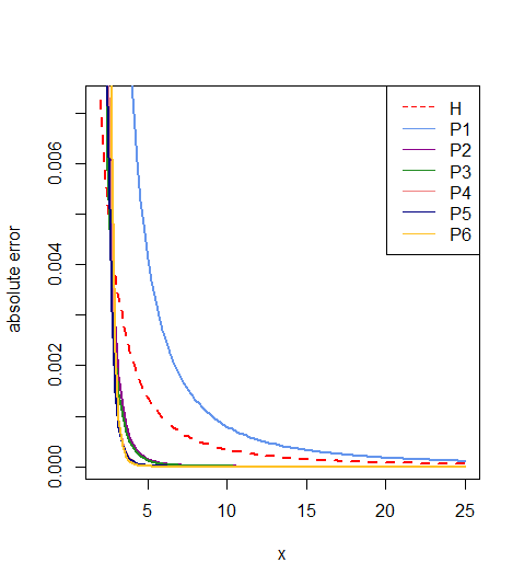
Refer to caption — Figure 1. The approximation accuracy of $H$ and $P_{n}$ .

Figure 1 shows the performance of approximations and we can see Hedges’ approximation $H(m)$ , which is the dashed red line, has less accuracy compared to $P_{2}(m),P_{3}(m),\cdots,P_{m}(m)$ . In terms of absolute errors, we can see

(3.3)

\delta_{6}(m)<\delta_{5}(m)<\delta_{4}(m)<\delta_{3}(m)<\delta_{2}(m)<\delta_{0}(m)<\delta_{1}(m).

This can also be verified by performing numerical analysis demonstrated by Table 1, from which the order of accuracy is more straightforward.

Table 1. Numerical accuracy of different approximations

\begin{array}[]{c c c c c c c c}\hline\cr m&\delta_{0}&\delta_{1}&\delta_{2}&\delta_{3}&\delta_{4}&\delta_{5}&\delta_{6}\\ \hline\cr 10&0.00033&0.00079&5.34e-06&4.66e-06&1.43e-07&1.35e-07&8.47e-09\\ 30&3.55e-05&7.49e-05&4.60e-08&4.03e-08&1.13e-10&1.067e-10&6.24e-13\\ 50&1.27e-05&2.62e-05&5.56e-09&4.86e-09&4.71e-12&4.45e-12&1.79e-14\\ 70&6.44e-06&1.32e-05&1.40e-09&1.23e-09&5.93e-13&5.60e-13&5.66e-15\\ 100&3.15e-06&6.39e-06&3.29e-10&2.88e-10&4.49e-14&4.11e-14&2.31e-14\\ 200&7.84e-07&1.58e-06&2.00e-11&1.75e-11&4.29e-14&4.29e-14&4.19e-14\\ \hline\cr\end{array}

4. discussion

In this paper, we have proposed a sequence of more accurate approximations to the multiplicative correction factor, $J(m)$ , in Hedges’ unbiased estimator of standardized mean difference.

It is also worth mentioning that the difference between $P_{5}(m)$ and $P_{6}(m)$ are small when $m$ is over 100, and there is almost no difference when $m$ is over 200. We can also see this from Figure 2, both $P_{5}(m)$ and $P_{6}(m)$ are osculating around 0 within the magnitude of $2\times 10^{-13}$ .

More accurate and efficient approximations to Hedges’ $g*$ would be available with deeper understandings of the properties of gamma functions, which has always been an appealing topic in both mathematics itself and our future work.

References

[1] Hedges, L. V. (1981) Distribution Theory for Glass’s Estimator of Effect size and Related Estimators, Journal of Educational Statistics, 6(2), pp. 107–128. doi: 10.3102/10769986006002107.
[2] Hedges, L. V., and Olkin I. (2014) Statistical Methods for Meta-Analysis. Academic Press.
[3] Borenstein, Michael, Larry V. Hedges, Julian P. T. Higgins, and Hannah Rothstein. (2009) Introduction to Meta-Analysis. Chichester, U.K. John Wiley and Sons.
[4] J. T. Chu, A modified Wallis product and some applications, Amer. Math. Monthly 69 (1962), no. 5, 402-404.
[5] C. Mortici,New approximation formulas for evaluating the ratio of gamma functions, Math. Comp. Modelling 52 (2010) 425–433.
[6] Dumitrescu, S.,Estimates for the ratio of gamma functions by using higher order roots, Studia Universitatis Babes-Bolyai, Mathematica . Jun2015, Vol. 60 Issue 2, p173-181. 9p.
[7] Paris, R. B. (2011). Asymptotic approximations for n!, Applied Mathematical Sciences.
[8] Xue, X. (2020) Estimation of within-study covariances in multivariate meta-analysis, arxiv:2003.05092.