The MALATANG Survey: Dense Gas and Star Formation from High Transition HCN and HCO+ maps of NGC 2532020The MALATANG Survey: Dense Gas and Star Formation from High Transition HCN and HCO+ maps of NGC 253–C
Abstract
To study the high-transition dense-gas tracers and their relationships to the star formation of the inner 2 kpc circumnuclear region of NGC 253, we present HCN and HCO maps obtained with the James Clerk Maxwell Telescope (JCMT). With the spatially resolved data, we compute the concentration indices for the different tracers. HCN and HCO+ 4-3 emission features tend to be centrally concentrated, which is in contrast to the shallower distribution of CO 1-0 and the stellar component. The dense-gas fraction (, traced by the velocity-integrated-intensity ratios of HCN/CO and HCO+/CO) and the ratio (CO 3-2/1-0) decline towards larger galactocentric distances, but increase with higher SFR surface density. The radial variation and the large scatter of and imply distinct physical conditions in different regions of the galactic disc. The relationships of versus , and SFE versus are explored. SFE increases with higher in this galaxy, which is inconsistent with previous work that used HCN 1-0 data. This implies that existing stellar components might have different effects on the high- HCN and HCO+ than their low- emission. We also find that SFE seems to be decreasing with higher which is consistent with previous works, and it suggests that the ability of the dense gas to form stars diminishes when the average density of the gas increases. This is expected in a scenario where only the regions with high-density contrast collapse and form stars.
Keywords:
galaxies: ISM – galaxies: individual: NGC 253 – galaxies: star formation – ISM: molecules – submillimetre: ISM1 Introduction
The important role of molecular gas in the star-formation process has received much attention from observational and theoretical studies (Kennicutt & Evans 2012; Krumholz 2014). In recent years, increasing samples of molecular-gas measurements of galaxies in both the local and the early universe (Carilli & Walter 2013; Kruijssen et al. 2014; Saintonge et al. 2017; Tacconi et al. 2018; Riechers et al. 2019) have shed new light on this topic. The evolution of the molecular-gas fraction (defined as the gas mass per unit stellar mass) is found to be surprisingly similar to that of the evolution of the cosmic star-formation-rate density, in the sense that they both show a peak at redshift 1 to 2 and decline in the local universe (Walter et al. 2014; Tacconi et al. 2018; Riechers et al. 2019). This indicates that throughout most of cosmic time, molecular gas is the crucial fuel for star formation and galaxy evolution.
However, it is still unclear how the physical and chemical parameters of the molecular gas affect the process of star formation. Specifically, how do we interpret the variations observed in the Kennicutt–Schmidt (KS) star-formation (SF) relationship (Kennicutt 1998), and how do the density and temperature of molecular gas relate to the star-formation rate (SFR), or the star-formation efficiency (SFE, defined as the SFR per unit gas mass)? Since the pioneering studies of Gao & Solomon 2004a; Gao & Solomon 2004b, it has been shown that the amount of dense molecular gas is tightly and linearly correlated with the SFR of individual galaxies (in logarithmic scale), where dense gas is usually defined as gas with a volume density cm-3, and can be traced by molecular emission lines with high critical densities () like HCN (Baan et al. 2008; Graciá-Carpio et al. 2008; Juneau et al. 2009; Lada et al. 2010; Greve et al. 2014; Liu et al. 2015b; Liu et al. 2015a; Zhang et al. 2014; Chen et al. 2015; Braine et al. 2017; Tan et al. 2018). Meanwhile, observations on smaller scales, such as of resolved galaxy structures or of molecular clouds in the Milky Way, also showed that star-forming sites are mainly associated with dense structures (Wu et al. 2005; André et al. 2014; Liu et al. 2016; Stephens et al. 2016; Shimajiri et al. 2017). Together with the extragalactic results, these studies suggest a simple threshold model where stars only form at gas densities above cm-3, and this model might be universal across eight orders of magnitude of the SFR (Lada et al. 2012; Evans et al. 2014). However, there is also a compelling model that does not require threshold density, and the dense-gas SF correlation can be explained as the association between young stars and nearby collapsing gas with a free-fall time comparable to the stars’ ages (Elmegreen 2015; Elmegreen 2018).
While the physical driver of the scatter along this dense-gas star-formation relationship likely relates to the feedback from star-formation or active galactic nuclei (Papadopoulos et al. 2014), we still lack enough samples to quantify this effect in different types of galaxies. More detailed analyses based on high-spatial resolution observations (Usero et al. 2015; Bigiel et al. 2016; Gallagher et al. 2018a; Gallagher et al. 2018b; Jiménez-Donaire et al. 2019) have revealed the variation of the SFR per unit dense gas mass (the dense-gas star-formation efficiency, SFE) in different regions of galaxy discs, and also in luminous infrared galaxies (Graciá-Carpio et al. 2008). Together, these results point to an alternative model that is turbulence regulated (Krumholz & McKee 2005; Krumholz & Thompson 2007).
Recent observations show that these molecules with high can also be excited in extended translucent regions () that are not actively forming stars (Pety et al. 2017; Watanabe et al. 2017; Kauffmann et al. 2017; Nishimura et al. 2017; Harada et al. 2019). This is evidence for the scenario pointed out by Evans 1999, that the effective density to excite a certain line can be much lower than the critical density, and one should be cautious about interpreting single-line observations, namely they are not adequate to accurately estimate gas density. So multiple transitions, especially high- lines, are necessary for a more-robust analysis of the relationship between dense gas tracers and SF. Previous studies have mainly used the ground transition of dense-gas tracers and our work aims to explore the behaviour of their high- transitions, allowing for the possibility to combine multiple transitions for the diagnosis of molecular gas in galaxies.
To bridge the gap between Milky Way clouds and galaxy-integrated observations, and to explore systematically the relationship between dense gas and star formation in nuclear versus disc regions, we carried out the MALATANG (Mapping the dense molecular gas in the strongest star-forming galaxies) large program on the James Clerk Maxwell Telescope (JCMT). MALATANG is the first systematic survey of the spatially resolved HCN and HCO+ emission in a large sample of nearby galaxies. Tan et al. 2018 presented the MALATANG data of six galaxies. They explored the relationship between the dense gas and the star formation rate and show that the power-law slopes are close to unity over a large dynamical range. They also imply that the variation of this relationship could be dependent on the dense-gas fraction () and dust temperature.
NGC 253 is the nearest spiral galaxy hosting a nuclear starburst ( = 3.5 Mpc, based on the planetary nebula luminosity function, Rekola et al. 2005). This makes it an ideal laboratory for detailed studies of the star-formation activity in an active environment, and it is accessible to most major facilities, such as the JCMT and ALMA. In Table 1 we list some adopted properties of NGC 253. High-resolution observations of molecular gas have found expanding molecular shells in the starburst region (Sakamoto et al. 2006), and star-formation activity may be suppressed due to the expulsion of molecular gas (Bolatto et al. 2013b). The molecular-gas depletion time () of NGC 253 is also found to be 5–25 times shorter than the typical disc values of other galaxies. The molecular-line emission is concentrated in the inner 1 kpc, and the dense molecular-gas tracers show clumpy and elongated morphologies, and they show excellent agreement with the 850-µm continuum down to very small scales of few parsecs (Leroy et al. 2015; Meier et al. 2015; Walter et al. 2017; Leroy et al. 2018). Earlier studies have presented multiple HCN and HCO+ observations in the nucleus of NGC 253 (Nguyen-Q-Rieu et al. 1989; Nguyen et al. 1992; Paglione et al. 1995; Paglione et al. 1997; Knudsen et al. 2007), and the average density of the gas is suggested to be 5105 cm-3 (Jackson et al. 1995). An excitation analysis revealed that the lines from both molecules are subthermally excited. Submillimeter Array (SMA) observations of HCN 4-3 toward the central kiloparsec of NGC 253 have shown that the dense-gas fraction is higher in the central 300 pc region than in the surrounding area (Sakamoto et al. 2011).
This paper is a follow-up to the MALATANG data of NGC 253 (this galaxy was included in the sample of Tan et al. 2018). We focus on the analysis of the variation in the parameters related to dense gas and star formation. In Section 2 the observations and data reduction are introduced. In Section 3 we present the spectra, images, radial distributions, and line ratios of the molecular lines. In Section 4 we discuss the relationship between SFE, and stellar components, and the dense-gas star-formation relationship.
| Parameters | Value | Ref. |
|---|---|---|
| R.A. (J2000) | 0047331 | (1) |
| Dec. (J2000) | 25°17′197 | (1) |
| Distance | 3.5 Mpc | (2) |
| Velocity (Heliocentric) | 243 2 km s-1 | (3) |
| Morphology | SAB(s)c | (4) |
| Diameter () | 27.5 arcmin | (4) |
| Inclination | 76 | (5) |
| Position angle | 51 | (5) |
| nuclear CO column density | 3.5 cm-2 | (6) |
| HI size (at 1020 cm-2 level) | 29 2 kpc | (7) |
| SFR | 4.2 M☉yr-1 | (8) |
2 Observations and Data reduction
2.1 JCMT HCN 4-3 and HCO+ 4-3 data
A total of 390 hours was spent on MALATANG observations from 2015 December and 2017 July (Program ID: M16AL007). The Heterodyne Array Receiver Program (HARP, Buckle et al. 2009) was used to observe HCN 4-3 and HCO+ 4-3. Two adjacent receptors (H13 and H14) on the edge of HARP were not functional, which caused a nonhomogeneous coverage for the jiggle-mode (see Fig. 1). In order to cover the major axes of the galaxies, the orientation of HARP was adjusted for each galaxy according to its position angle, so that four receptors lined up along the galaxy’s major axis. For NGC 253, the inclination of its galactic disc is 76 (north is the receding side), and the position angle of its major axis (measured counter-clockwise from north) is about 51 (Jarrett et al. 2003).
The Auto-Correlation Spectral Imaging System (ACSIS) spectrometer was used as the backend, with 1 GHz bandwidth and a resolution of 0.488 MHz, corresponding to 840 and 0.41 km s-1at 354 GHz, respectively. The half-power beam width (HPBW) of each receptor at 350 GHz is 14 arcsec, corresponding to 240 pc linear resolution at the distance of NGC 253. The telescope pointing was checked on R Scl (R Sculptoris) before observing our target source and subsequently every 60 to 90 minutes, using the CO 3-2 line at 345.8 GHz. The uncertainty in the absolute flux calibration was about 10 per cent for galaxies and was measured using standard line calibrators. The details of the survey description, sample, and data are given in Zhang et al. (in prep., see also Tan et al. 2018).
Two observing modes were used to observe NGC 253. To fully map the central 22 arcmin region (centred at R.A.(J2000.0) = 0047331, Dec(J2000.0) = 25°17′197), the 33 jiggle observing mode was used, with a grid spacing of 10 arcsec. This was mostly done in 2015 December in excellent weather conditions, i.e., mean and 0.036 for HCN 4-3 and HCO+ 4-3, respectively. The integration times spent in jiggle mode for the HCN and HCO+ lines were 142 and 100 minutes, respectively. To reach deeper integrations in the outer parts of NGC 253, the stare observing mode was used and the tracking centre was at (J2000.0) = 0047348, Dec(J2000.0) = 25°17′008, which was shifted by 30 arcsec to the north-east along the major axis of NGC 253. The grid spacing was 30 arcsec (see Fig. 1). The integration times spent in stare mode for HCN 4-3 and HCO+ 4-3 were 7.8 and 6.1 hours, respectively.
2.2 Ancillary data
Ancillary data of CO 1-0 and CO 3-2 were obtained for a more-comprehensive analysis of the interstellar medium in NGC 253. The CO 1-0 data are from the Nobeyama CO Atlas of Nearby Spiral Galaxies (Sorai et al. 2000; Kuno et al. 2007), and the CO 3-2 data from the JCMT archive (project ID: M08AU14). We also include infrared archival imaging data from Spitzer (IRAC 3.6 µm and MIPS 24 µm), and Herschel (PACS 70, 100, and 160 µm). The Nobeyama and Herschel data were convolved to 14-arcsec resolution and regridded to the same pixel scale (see Tan et al. 2018 for more details of the processing of the ancillary data). This allowed us to calculate the total infrared luminosity (8–1000 µm) in each pixel using a combination of the 24-, 70-, 100-, and 160-µm luminosities (Galametz et al. 2013; Tan et al. 2018).

2.3 Data reduction
The starlink (Currie et al. 2014) software package was used to reduce the JCMT data. Some of the receptors, mostly the outer ones, were not very stable during some observing scans, and spikes and an unstable baseline can be seen in some of the raw data. To enhance the signal-to-noise (SNR) ratio, we first checked the raw data by eye with the gaia tool (part of starlink) and flagged the particularly bad sub-scans. Secondly, the parameters for the orac-dr pipeline (Jenness et al. 2015) were adjusted to remove spikes and strong ripples further. This step was especially necessary for the CO 3-2 data because this line is too strong and wide, so there are not enough line-free channels for the default parameters to do proper baseline fitting, and we need to adjust the parameters. Thirdly, the pipeline was run again to compare with previous results. This way, we could better deal with the baseline correction and reveal weak signals in some regions of the final products. The final data are smoothed to a velocity resolution of km s-1, and the typical corresponding RMS noise is 7–10 mK for spectra obtained in jiggle-mode, and 2 mK for spectra obtained in stare-mode (Fig. 12).
The maps of NGC 253 were regridded to a pixel size of 10 arcsec. Fig. 12 shows the corresponding spectra of the central 13 7 pixels, including CO 1-0, CO 3-2, HCN 4-3, and HCO+ 4-3. Other pixels in the outer regions of the galaxy disc are mostly non-detections with relatively high noise, due to the relatively poor performance of the outer receptors of HARP.
The final maps were converted to the CLASS format and spectra were measured with the Gildas package11 1 http://www.iram.fr/IRAMFR/GILDAS/. The spectral intensity units were converted from antenna temperature to main-beam temperature using , where the main-beam efficiency = 0.64 22 2 https://www.eaobservatory.org/jcmt/help/workshops/.
To identify detections of the emission lines used in this work, we adopted the same criteria as Tan et al. 2018, i.e., we require that the integrated line intensity to be at least three times the "integrated noise" (SNR > 3). The uncertainty, , on the integrated line emission is:
| (1) |
where is the RMS of the spectrum given a spectral velocity resolution , is the velocity range used to integrate the line emission, and is the velocity width used to fit the baseline. Since CO lines are much stronger than HCN 4-3 and HCO+ 4-3 lines, and the emitting region of CO is probably larger than the regions dominated by these dense-gas tracers, but they still share the same kinematics and are covered by similar telescope beam size in general, despite their distinct spatial scales. So the velocity widths of the CO 1-0 and/or CO 3-2 lines are used as a reference for the velocity ranges of the HCN 4-3 and HCO+ 4-3 lines, especially for positions with low SNR. This way we can use the width to estimate upper limits (3) to the integrated intensities. In Table 3, we list the integrated intensities , , , and , and their ratios, for every pixel in Fig. 12. In Table 4 we list the line luminosities of HCN 4-3 and HCO+ 4-3, the SFR, and their dense-gas mass (). In accordance with (Tan et al. 2018), we calculate the line luminosities (, , and in this paper) in units of K km s-1pc2 and SFR based on the following equations:
| (2) | ||||
| (3) |
The infrared luminosity is calculated from
| (4) |
where is the resolved luminosity in a given band in units of and measured as , and are the calibration coefficients for various combinations of and Tan et al. 2018. The stellar surface density is calculated via:
| (5) |
3 Results
3.1 Spectra
Fig. 12 shows the HCN and HCO+ 4-3 spectra at every 10-arcsec pixel position within the central 13070 arcsec of NGC 253. The figure also shows the CO 1-0 and 3-2 spectra at the same positions. The CO spectra have been scaled down by a factor of 20 in order to better compare the profiles with those of HCN and HCN+. The 10-arcsec pixel size is the same as the beam spacing of the observations, and results in a slightly undersampled map. In the central pixel, the two dense-gas tracers are comparable to 1/20 of the peak intensity of CO 1-0, but in pixels away from the centre, the relative strengths of HCN and HCO+ 4-3 quickly drop. The typical peak intensity ratio between HCN 4-3 (or HCO+ 4-3) and CO 1-0 that we can detect is about 1/100 in the outer parts. In Section 3.3 and Fig. 5 the radial profiles of these tracers are presented.
The different tracers have similar spatially integrated line centres and widths, indicating that they originate from similar large-scale emitting regions. However, their line profiles are different in many regions of the map. The line centres of CO 1-0 can be different from those of the other tracers by 100 km s-1 in some pixels, while the line centres of CO 3-2 are closer to those of HCN 4-3 and HCO+ 4-3. While this difference is likely a result of the large optical depth of CO 1-0, it could also be caused by the different excitation conditions of the emissions. CO 3-2 traces warmer and denser gas than CO 1-0, and its emission regions would be more similar to those of HCN 4-3 and HCO+ 4-3. High-spatial-resolution ALMA observations in the central 1.5 kpc region of NGC 253 (Meier et al. 2015; Leroy et al. 2015) have shown that the morphologies of these molecules are quite different, in the sense that dense-gas tracers are more compact and clumpy, while CO is much more diffuse and extended. The measurements of the line intensities and their ratios are presented in Table 3.
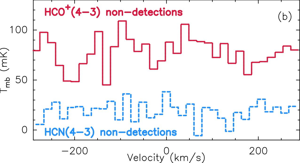
Fig. 2 shows the averaged spectrum (weighted by RMS) of the central 53 pixels (top panel) and the stacked spectrum of those non-detections (bottom panel). The central 53 pixels contain 90 per cent of the total flux of HCN 4-3 or HCO+ 4-3. This total value will be used as a global measurement later in Fig. 9. The stacking of non-detections yields spectra with RMS 0.6 mK for HCN 4-3, and mK for HCO+ 4-3, respectively, and there is no sign of a robust signal. Assuming a 200- km s-1 linewidth, the 3- integrated intensities correspond to 106.0 M☉ and 106.2 M☉, respectively.
3.2 Images of integrated intensities and their ratios
Fig. 3 shows maps of the integrated intensities (moment zero) of the different tracers used in this work. Contours starting from 30 per cent (0.2 dex) of the peak are overlaid. Although our observations are limited by resolution and sensitivity, the differences in compactness between tracers are significant. , HCN 4-3 and HCO+ 4-3 show the most-compact morphology, while CO 1-0 is the most extended. A quantitative comparison and analysis are presented in Section 3.3.
Fig. 4 shows maps of the ratios of different tracers, among which HCN 4-3/CO 1-0 (hereafter ) and HCO+ 4-3/CO 1-0 (hereafter ) can be treated as proxies for the dense-gas fraction, i.e., and are proportional to (), but bear in mind that the accuracy is largely limited by the conversion from line flux to mass (Usero et al. 2015), for both the dense gas (traced by HCN and HCO+), and CO. We will discuss this in more detail in Section4.1. It is obvious that traced by either or is much higher at the galaxy centre, and drops quickly toward the outskirts. The integrated-intensity ratios in the centre are generally 0.06. The integrated-intensity ratio of CO 3-2 and CO 1-0 (hereafter ) is shown in Fig. 4c. This ratio shows an interesting asymmetric morphology, which might be a result of the molecular outflow that was reported by Bolatto et al. 2013b, though the outflow does not seem to affect the dense gas, as judged from those images related to HCN or HCO+. We will further discuss this in Section 3.4.
/ can be treated as the molecular-gas star-formation efficiency, SFE SFR/ ( is the depletion time scale of the total molecular gas), while / and / can be proxies of SFE. In Fig. 4 they are shown in the last three panels (d-f). We can see that, first, the peak of SFE is on the (0,10) pixel in panel d. Second, SFE shows a more asymmetric morphology than SFEin panel e and f. Third, regions to the upper side (north-west) of the nuclei show about 0.5 dex higher SFE than the values in the centre. A similar behaviour was reported for M 51, i.e., the SFE traced by / shows a peak on its northern spiral arm (Chen et al. 2015). We can tell from Fig. 3 that HCN 4-3 and HCO+ 4-3 peak in the centre, so the asymmetric morphologies of SFE might be mainly caused by the stronger to the upper side (north-west). This implies that the of both the total molecular gas and the dense gas in the north-west of the galaxy centre is shorter than that of other regions of NGC 253. The asymmetric distribution of and SFE could be attributed to the structure of the interstellar medium of the nuclei. Bolatto et al. 2013b reported an expanding molecular outflow in the centre of NGC 253, and their data showed that the CO luminosity is approximately split between the north (receding) and the south (approaching) sides of the outflow. On the other hand, H emission is predominantly seen on the south side, and it is invisible on the north side probably due to obscuration. Therefore, as shown in Fig. 3e, infrared emission might dominate the north (receding) side, possibly because of more abundant dust than on the south (approaching) side. Our data are limited by modest resolution, and future works combining H and infrared data might help us more accurately estimate SFE and SFE in the circumnuclear region of NGC 253.
| tracer | (kpc) | (kpc) | / |
|---|---|---|---|
| CO 1-0 | 0.78 (0.15) | 0.38 (0.05) | 2.07 (0.48) |
| CO 3-2 | 0.68 (0.07) | 0.30 (0.01) | 2.26 (0.27) |
| HCN 4-3 | 0.58 (0.15) | 0.14 (0.01) | 4.00 (1.10) |
| HCO+ 4-3 | 0.54 (0.18) | 0.10 (0.01) | 5.29 (1.91) |
| 0.68 (0.12) | 0.33 (0.02) | 2.06 (0.39) | |
| stellar | 0.87 (0.13) | 0.37 (0.04) | 2.36 (0.44) |
3.3 Radial profile and concentration index
Fig. 5 presents the radial profiles of all the tracers used in this work. The radial distances are corrected for inclination, but note that all pixels come from a highly elliptical beam and many are not independent measurements of emitting regions in the disc, so the profiles shown here are only indicative. Only pixels with SNR3 are included. We highlight those data points along the major axis with red filled circles to guide the eye, and we find that they follow the main trend of most data points.
To obtain an averaged profile of each tracer, we calculate the mean intensity within every 0.17-kpc distance bin (the beam spacing along the major axis), weighted by their measurement error. The uncertainty of the mean value is calculated following equation (9) of Gallagher et al. 2018a, taking into account the error of each data point, and the number of pixels within each bin:
| (6) |
where is the uncertainty of the binned intensity, is the number of pixels in the bin, and is the oversampling factor accounting for the nonindependence of the pixels. = 1.4 in our work as the pixel size is 10 and the resolution is 14).
It is interesting to see that, while all the tracers’ intensity distributions show significant decreasing trends towards larger radii, CO 3-2, , HCN 4-3, and HCO+ 4-3 seem to have steeper gradients than CO 1-0 and the stellar component traced by 3.6-µmemission. For example, at 0.5 kpc from the galaxy centre, the integrated intensities of CO 3-2, , HCN 4-3, and HCO+ 4-3 are only approximately 10 per cent of those in the centre. For comparison, the integrated intensities of CO 1-0 at 0.5 kpc is about 30 per cent of the central value (also see Fig. 3). The difference indicates that, the spatial distribution of CO 1-0 is the most extended among all the tracers. While CO 1-0 emission comes from the cold and diffuse molecular gas, CO 3-2 and the two dense-gas tracers require denser and warmer gas, which tends to reside in the galaxy centre. This is also the case for the infrared emission, which traces cold dust emission that is closely associated with star-formation activity.
To establish a quantitative method to analyse the radial profiles of the different tracers observed in NGC 253, and to further apply this to the other sources of the MALATANG survey in our future works, we fit the concentration indices to the radial distributions (de Vaucouleurs 1977; Li et al. 2011). For HCN 4-3 and HCO+ 4-3 only detections with radial distance kpc are included in the fits (see Fig. 16). and are the radii that encompass 90 and 50 per cent of the total flux of each tracer, respectively. The total flux is derived from fitting the asymptotic intensity of a curve of growth, following the method of Muñoz-Mateos et al. 2009. In Fig. 16 we show two examples of how the curve of growth and the asymptotic intensities are derived.
The fitted parameters are listed in Table 2. HCN 4-3 and HCO+4-3 appear to have smaller than the other tracers, and they also show significantly higher concentration indices. Note that our resolution is 0.24 kpc so the observed values are spatially smoothed, which might not reflect the intrinsic concentration parameters. Leroy et al. 2015 used high-resolution (FWHM 2 arcsec) data of NGC 253 in the 3 mm band, and they derived and for CO 1-0 (0.4 and 0.15 kpc). These values are lower than ours (0.78 and 0.38 kpc), but the ratio / is similar. For dense gas, they derive and (0.3 and 0.1 kpc, respectively) by averaging the 1-0 transitions of HCN, HCO+, and CS. Note that their dense-gas observations lack short spacings data, so certain amount of emission on large spatial-scales is missing. As a result their and might be overestimated. If we average the and for HCN 4-3 and HCO+ 4-3, we get 0.54 and 0.12 kpc, respectively. We note that the telescope beam ( kpc) is larger than the fitted of HCN 4-3 and HCO+4-3, so they have large uncertainties and are likely overestimated by our data. This implies that the dense-gas tracers might be too compact for the JCMT to resolve their . Moreover, we speculate that, since the higher transition lines are excited in more-compact clumps with higher gas density, their and should be smaller while the ratio / might be higher, compared with their low- lines.
The emission lines require higher excitation temperatures and higher critical densities, and in regions with different kinematic temperature (), the effective critical densities () for the excitation of a certain line will change dramatically (Evans 1999). Thus the large scatter between the centre and disc regions not only reflects the change in dense-gas abundance, but it could also be a result of the distinct excitation environments. While few studies have explored the optical depths of dense-gas tracers in galactic disc regions, they have been suggested to be optically thick in galaxy centres (Greve et al. 2009; Jiang et al. 2011; Jiménez-Donaire et al. 2017) and nearby ULIRGs (Imanishi et al. 2018). At this stage it is still unclear whether HCN and HCO+ are optically thin in galactic disc regions. So the profiles shown here do not necessarily reflect their column densities. Accurate estimates of the gas temperature and optical depth of these lines are needed to reveal the true population distribution of spectral energy levels and their excitation conditions.
Note that the analysis using radial profiles is based on the simplified assumption that regions with the same galactocentric distances have similar properties. This is not always the case, especially substructures such as rings, bars and spirals in the circumnuclear regions cannot be well recovered by this approach. Radial profiles are useful diagnostics for samples with intermediate-to-low spatial resolution, but we note that they can only serve as a first-order approximation for the relationships between physical properties and galactocentric distance. The result presented in this paper is uncertain and only indicative , and we look forward to investigating this method for large samples in future studies at higher resolution.
3.4 Line ratio and dense-gas fraction
Tan et al. 2018 reported the integrated-intensity ratios of and in different regions of six galaxies. The ratios lie between approximately 0.003 and 0.1, and they are higher in the centre and lower in outer regions. Take in galactic centres for example, among their six galaxies, NGC 1068 and NGC 253 (a possibly weak AGN, Müller-Sánchez et al. 2010) have the highest ratios in the nuclei which are slightly less than 0.1. In IC 342, M 83, and NGC 6946, the ratios in the nuclei are about 0.01 to 0.015. In the starburst galaxy M 82, the nuclear ratio is about 0.02 (see fig. 5 in Tan et al. 2018 for more details). Gallagher et al. 2018a also resolved and of four local galaxies, and their ratios are also in a similar range, while appears to be modestly higher than in general (see their fig. 9). For more discussion of the line ratios and their implications, refer to Izumi et al. 2016 and references therein.
In Fig. 6 we show the radial profiles of the integrated-intensity ratios of the molecular lines used in this work. The ratios of and are, to first order, proportional to the dense-gas ratio , and we emphasize that here is different from that traced by HCN 1-0 and HCO+ 1-0, since the different transitions require different densities. Similar to Fig. 4, peaks in the centre, but drops quickly to only about one sixth of the central value at 0.5 kpc. This is consistent with the result from Jackson et al. 1995 that the most highly-exited gas is confined to the inner 0.5 kpc nuclear region. They implied that the density distribution of the molecular gas is distinct in the circumnuclear region, where the high-density-gas fraction is likely to be several times higher than in the outskirts. In other words, compared with most of the galaxy disc, high-density gas (possibly in the form of clumps) resides preferentially in the galaxy centre. This plot of the decreasing with radius in the galactic disc also implies that the filling factor of dense gas is much smaller than that of the bulk of molecular gas traced by CO (Paglione et al. 1997; Leroy et al. 2015). Thus we suggest that for extragalactic observations telescopes with a smaller beam are more suitable to detect dense-gas emission, as larger beams might suffer more from beam dilution.
The CO 3-2/1-0 ratio () as a function of radius is also shown in Fig. 6. It is obvious that drops quickly at larger radii, similar to the decreasing trend of . is close to one in the centre, which is several times higher than the at 1 kpc (). We also note in Fig. 4c that on a few pixels to the west side of the centre, is higher than the value at the (0,0) position. The pixel on the south-west (10 arcsec to the right side of the disc) of the centre appear to be coincident with the position of the CO outflow reported by Bolatto et al. 2013b. Compared with CO 1-0, CO 3-2 emission requires a higher excitation temperature and a higher critical density, so gives important information on the excitation conditions of the molecular gas.
In previous studies, and (CO 2-1/1-0 ratio) have been reported and are widely used to convert and to to estimate the total molecular-hydrogen mass (Leroy et al. 2009; Mao et al. 2010; Wilson et al. 2012). was reported to be in the range 0.2–1.9 (mean value = 0.81) in galaxy-integrated observations (Mao et al. 2010). In resolved observations of nearby galaxies the mean is found to be 0.18 with a standard deviation of 0.06 (Wilson et al. 2012). Our values of lie in the range from these works, and the variation of in the central region of NGC 253 shows that this ratio is obviously dependent on galactic environments. In strongly star-forming galactic centres where the conditions resemble those in luminous infrared galaxies (LIRGs), CO 3-2 emission is easily enhanced and is naturally much higher than in the quiescent environment of discs (Mao et al. 2010). We suggest that the scatter of among galaxies is a natural result of the variation of among different regions of any single galaxy. For single-dish observations that do not resolve the molecular gas of galaxies, one can only obtain a spatially averaged , and in galaxies with more denser and warmer molecular gas, such as LIRGs, the averaged tends to be higher. Also, the filling factors of CO 3-2 and CO 1-0 for single-dish observations are dependent on the physical scale covered by the beam, and this observed effect can also contribute to part of the scatter of the observed . If and are used to convert and to to estimate the total molecular-hydrogen mass, we caution that one must take into account the variation of or as an important uncertainty in the conversion.
Fig. 7 plots line ratios as a function of SFR surface density, , so as to explore the relationships of versus , and versus . In Fig. 7a, appears to increase for higher , especially when we only look at data points along the major axis (circles). Limited by the SNR we could not obtain reliable in the lower regime, where most of the data points come from the outer disc region. On the other hand, we have relatively higher SNR for the two CO lines, so in the bottom panel we are able to show in all pixels used in this work, and to explore the lower- regime. We can see that shows smaller scatter in the lower- regime, and its scatter increases significantly with increasing . For pixels with , is mostly lower than 0.5, while near the galaxy centre is about 100 times higher and can be as high as 1.5. Again note that a few pixels have higher than the central pixel, and they are coincident with the position of the CO outflow reported by Bolatto et al. 2013b. In Fig. 4 we also note that the map exhibits an asymmetric morphology. Thus we speculate that the molecular outflow might dominate the large scatter in the higher- regime of the plot and the more-active environment in the central pc region.
The two plots in Fig. 7 suggest that and are more likely to be higher in regions with higher , i.e., the more-active environment in the central pc of NGC 253. However, there are also regions with high accompanied with low and low . Considering that SFR is more directly related to the mass of dense/warm gas, we expect to see tighter correlations between HCN (or HCO+) and (see Section 4.1), as well as between CO 3-2 and (Wilson et al. 2012). So we speculate that the scatter in and is likely caused by the variation of the CO intensity among different regions.
4 Discussion
The spatially resolved dense-gas emission of NGC 253 enables us to analyse how the galactic environment affects the relationship between dense gas and star formation (Usero et al. 2015). In the following, we will first discuss the dense-gas star-formation relationships, and how varying dense-gas conversion factors affect the relationships. Then the role of stellar components in the dense-gas fraction and the dense-gas star-formation efficiency, SFE is discussed in Section 4.2.
4.1 Dense-gas star-formation relationship
Tan et al. 2018 discussed the dense-gas star-formation relationship, using the six galaxies of the MALATANG sample that were mapped by JCMT. The whole sample shows a linear correlation between log10 and log10, and for HCN 4-3 the fitted slope is nearly unity. However, the scatter about the relationship is not negligible, and the slopes are likely different among individual galaxies. Such a variation in the ratio of the SFR and the mass of the dense molecular gas () suggests a varying star-formation efficiency, as discussed in recent studies (Usero et al. 2015; Gallagher et al. 2018a).
Shimajiri et al. 2017 derived an empirical relationship between the dense-gas conversion factors and the local far-UV radiation field, , which can be derived from Herschel 70- and 100-µm intensities. Here we adopt this varying conversion factor for our data and compare it with a constant to revisit the dense-gas SF relationship in NGC 253, using the full mapping data of HCN 4-3 and HCO+ 4-3 with 0.24-kpc resolution. Hereafter we use to distinguish it from the constant used by Gao & Solomon 2004a; Gao & Solomon 2004b and most other studies. To explore how the dense-gas conversion factors affect the relationship, two sets of are calculated based on and the constant , respectively, then we compare the relationships plotted for the different . Note that this approach relies on the assumption that NGC 253 conforms to Milky Way values in terms of gas and dust properties, but there is a large uncertainty in this assumed similarity. Please see Leroy et al. 2018 and Knudsen et al. 2007 for comparisons of star-forming properties between NGC 253 and the Milky Way.
We adopt the following relationships from Shimajiri et al. 2017:
| (7) |
| (8) |
is calculated from Herschel/PACS 70- and 100-µm data (here B is the bandwidth of the Herschel/PACS filters at 70 and 100 µm):
| (9) |
where:
| (10) | ||||
Our calculation shows that the median of in NGC 253 is M, which is a factor of 2.5 higher than the constant conversion factor, = 10 M, used in previous studies (Gao & Solomon 2004a; Wu et al. 2005). We adopt a luminosity ratio of 0.3 to convert from to for HCN and HCO+ following Tan et al. 2018. In Fig. 8 we plot SFR as a function of . In the left panel, is calculated using the varying , while the right panel uses the constant = 10. The Bayesian method coded in the idl routine linmix_err provided by Kelly 2007 was used for linear regression of the data. The method accounts for both uncertainties and upper limits. This is important especially for observations of the weak molecular lines, of which a significant part of the measurements have low SNR, as other methods not accounting for upper limits are biased to high-SNR data. The density distributions of the fitted slopes are shown as insets in the plot. Following Kelly 2007, the posterior median is adopted as an estimate for the parameter, and the median absolute deviation of the posterior distribution is used as an error of the parameters.
Comparison between the two panels of Fig. 8 shows that, when adopting , slopes of the dense-gas SF relationship become much steeper than those based on the constant . (HCN) and (HCO+) are and for constant , while we obtain, and , respectively, when adopting . The difference between the two sets of data is mainly caused by data points with lower SFR, for which values become 0.5 dex higher than estimated from fixed .
Although the dynamic range of our data for NGC 253 is limited to three orders of magnitude, Fig. 8a shows a nearly linear correlation between SFR and for both HCN 4-3 and HCO+ 4-3. The difference between our fitted slopes and those demonstrated based on a much larger dynamic range (Tan et al. 2018, e.g.,) is within the fitted errors. However, while the relationship based on shows a strong correlation, it is obviously not a one-to-one relationship. In addition to the uncertainty in the conversion factors themselves, the luminosity ratio between 4-3 and 1-0 transitions of HCN and HCO+(/) that we adopt might also be a major source of uncertainty, since in the galaxy centre / is probably higher than in the disc (Tan et al. 2018). Also note that the excitation conditions and density distribution of the molecular gas are not well constrained, so discussions based on high transition emission line alone is far from accurate for revealing the physical properties of star-forming gas. In Fig. 8a we therefore plot in addition the line luminosity on the top x-axis to show the actual measurements.
In Fig. 9 we show a updated version of the SF relationship from Tan et al. 2018, using NGC 253 HCN 4-3 data from this paper, and new HCN 4-3 data of LIRGs from Imanishi et al. 2018. Instead of and used in Tan et al. 2018, here we use SFR and . In Fig. 9, the black solid line ( = 1.08 0.01) is given by the Bayesian method linmix_err, and the blue dashed line is the same fit for NGC 253 data alone (from Fig. 8a, using the constant ). We can see that the fit for NGC 253 is slightly shifted from the overall fit, suggesting that for certain they tend to have lower SFR (by about 0.2 dex), or the overall SFE in NGC 253 is lower. Jackson et al. 1995 suggested that the overall gas density in NGC 253 is at least 10 times higher than that in M 82. So it is likely there is more dense gas in NGC 253, and this could explain the higher at certain SFR comparing with M 82 in this plot. Finally, it is worth noting that with higher resolution we are looking at smaller regions in galaxies, and the scatter would become more prominent, due to the fact that star-formation events in these regions take place during different epochs. Therefore, less dispersion is expected in correlations using data from entire galaxies where we see averaging values of parameters, although rare excursions can be also observed (Papadopoulos et al. 2014).
The uncertainty associated with converting the CO emission to the mass or column density of the total molecular gas ( or ) has been extensively studied. is likely affected by a number of physical conditions, such as the value of the gas surface density in giant molecular clouds, , the brightness temperatures of the emitting gas, the distribution of GMC sizes (Bolatto et al. 2013a), the effect of cosmic rays and the metallicity. Although is poorly constrained, at least qualitatively, the environment must also play a role in the uncertainty in the mass-to-light ratio of dense-gas tracers. We note that adopting in Fig. 8 relies on an assumption that the empirical relationship between and FIR intensity proposed by Shimajiri et al. 2017 holds for our observations on sub-kpc scales. However, it is unclear how to quantify the effect of the radiation field on across 200 pc scales. Calibrations of are beyond the scope of this paper, but we note that high spatial resolution and multiple-transition data of the dense-gas tracers together might provide more information about the parameters necessary for calibrating , such as surface density, brightness temperature, and the sizes of dense clumps. With regard to theoretical models that may explain variations in and SFE, see Usero et al. 2015 for a thorough discussion.
4.2 The relationships between star-formation efficiency, dense-gas fraction and stellar components
Previous studies have used HCN 1-0 as a dense-gas tracer and showed that the existing stellar component affects the parameters related to dense-gas emission. (Usero et al. 2015; Bigiel et al. 2016; Gallagher et al. 2018a; Jiménez-Donaire et al. 2019). They report decreasing trends in both SFE versus , and SFE versus , i.e., stellar surface density. With our JCMT HCN 4-3 and HCO+ 4-3 data, and stellar surface densities derived from Spitzer 3.6-µm data we can test such scaling relationships in this work.
In Fig. 10 we plot SFE versus and SFE versus to explore how affects the SFE for the total molecular gas and dense molecular gas, respectively. The data from Usero et al. 2015 is shown as purple diamonds in the plots. We convert the to the luminosity in these plots assuming / = 0.3. Considering the systematic differences that their sample used HCN 1-0 and CO 2-1, the regression fits are only applied to our sample. For the relationship of SFE versus (Fig. 10a), we do not see any statistically significant correlation between the two parameters. Note that in the subsequent analysis we only adopt data points with SNR3. This is because, unlike the star-formation relation (Fig. 9) which is a rather simple log-linear fit (based on many previous studies), for the other relations it is unclear what kind of relation holds between the two parameters. So upper limits can not be include in the analysis, and we only use spearman coefficients and hypothesis test to discuss whether they have potential correlations. The lines in the plots are Local Polynomial Regression fits only to guide the eye, which is similar to the binning method used in many other studies, and they do not strongly suggest that our data points closely follow those fits. This is consistent with Usero et al. 2015 and the larger galaxy sample compiled by Gallagher et al. 2018a, where they show a very weak correlation ( = 0.13) and a large scatter about the relationships, and they suggest that the HCN/CO ratio is a relatively poor predictor of SFE. Our plot shows a similar case using high- dense molecular lines, implying that the SFE, if measured as SFR per unit total molecular gas (SFE) is rather independent of the dense-gas fraction () that is measured with the transition. Furthermore, such a large scatter reported in our work and other studies indicates that a higher SFE (or shorter molecular-gas depletion time) does not necessarily correspond to a higher , thus the real star-formation scenario might be more complicated than the simple model proposed by Lada et al. 2010.
In Fig. 10b we explore the relationship between the dense-gas star-formation efficiency (SFE) and . We see plausible decreasing trends, which are consistent with Usero et al. 2015, and their fitted slope is shown as a purple line in Fig. 10b for comparison. The anti-correlations are not statistically significant, and we note that the trends might be partly attributed to the correlation between and (similar to the Kennicutt–Schmidt law relating the gas content and SFR), since is partially cancelled out in this SFE– relationship. It is interesting to see the data points of Usero et al. 2015 appear to be consistent with our data. In Fig. 10a they together suggest that there is no significant correlation between SFE and . In Fig. 10b their sample also lies in the same range, although our HCN data do not follow their fitted slope (purple dashed line). Note that they derived the CO 1-0 luminosity from converting CO 2-1 emission assuming = 0.7, and that our data also rely on the assumption of / = 0.3. It is therefore likely that the two samples have systematic differences caused by the conversion between different transitions. Our data follow the same prediction given by the model used in Usero et al. 2015 for a fixed average gas volume density cm-3. As pointed out in Section 3.4, dense-gas tracers are so compact compared with the single-dish beam that is dependent on the observing resolution, and we need high-resolution data, e.g., from ALMA, to truly understand these scaling relationships related to .
In Fig. 11 we explore how and SFE are affected by . In Bigiel et al. 2016, where HCN 1-0 was used, an increasing trend between and , and a decreasing trend between SFE and are reported. They were interpreted as the effect of interstellar-gas pressure (traced by the stellar surface density) on the gas-density structure, in the sense that high pressure would increase the overall mean density of the interstellar gas. Thus the HCN 1-0 intensity and are both elevated, but the density contrast, which is defined as the difference between the high-density peaks and the mean density, is reduced. SFE is controlled by the prevailing contrast, so it is also reduced in environments with higher pressure.
Fig. 11a shows that traced by both HCN 4-3 and HCO+ 4-3 seems to be weakly correlated with , with Spearman correlation coefficients (HCN) = 0.23 and (HCO+) = 0.29, respectively, but hypothesis tests show that they are not statistically significant ( 0.05). This is likely due to our limited data for only one galaxy, and the variation of is large, especially in the log10 range between 2.5 and 3. If we compare our data points with previous studies (Gallagher et al. 2018a; Usero et al. 2015), they seem to lie in a similar range in the plot, though we are using high- lines.
With regard to the relationship between SFE and , previous studies using the transition of HCN and/or HCO+ all showed anti-correlations (Usero et al. 2015; Gallagher et al. 2018a; Jiménez-Donaire et al. 2019), so it is somewhat surprising to see an increasing trend between SFE and in Fig. 11b. The Spearman correlation coefficients are (HCN) = 0.65 and (HCO+) = 0.71, respectively, and they are statistically significant ( 0.05). Running lines from polynomial fits are shown just to guide the eye. The increasing trend between SFE and in Fig. 11b is consistent with the star-formation scenario that the stellar component plays an important role in regulating the local SFR, as the gravitational potential is dominated by the stellar mass and therefore is deeper near the centre. Thus it increases the hydrostatic gas pressure in the disc and reduces the free-fall time for gas to collapse. Therefore the SFE is likely enhanced in star-dominated regions (Ostriker & Shetty 2011; Shi et al. 2011; Meidt 2016; Shi et al. 2018).
We speculate that the inconsistency between Fig. 11b and similar results in previous studies could be explained by observational and/or physical effects. Observationally, the argument by Bigiel et al. 2016 relies heavily on the large number of low-SNR data points and upper/lower limits, at least in the low regime (102.5 M☉ pc-2). In contrast, in Fig. 11 our statistics only include data points with SNR 3. However, their latest result based on a larger sample shows more promising trends (Jiménez-Donaire et al. 2019), so the difference is more likely a physical effect. The inconsistency implies the possibly different effects of on HCN 4-3 and HCO+ 4-3. At this stage, it is difficult to quantify the relationship between stellar surface density (gas pressure) and average gas density or density structure, and the actual relationship between SFE and local physical conditions, such as might be more complicated. Qualitatively, high- lines require higher critical densities and higher excitation temperatures, which are only met in a small part of the gas structure, i.e., the highly concentrated molecular clumps. Thus they might be less sensitive to the change in the overall density structure compared with low- lines. As proposed by Bigiel et al. 2016 high means high gas pressure, which would raise the overall average gas density and decrease the density contrast traced by HCN 1-0. As a consequence, low- dense molecular lines no longer only trace the gas undergoing star formation, and this is their explanation for the decreasing SFE(HCN 1-0) with increasing . On the other hand, the high- lines might still trace the "density contrast" properly thus they are good tracers of the molecular gas undergoing star formation.
Leroy et al. 2017 show that the emissivity of the high-density tracers () depends strongly on the density distribution of the gas, and the corresponding line ratios can reflect the change in the gas-density structure. Therefore the difference between Fig. 11(b) and the graphs by Bigiel et al. 2016 and Gallagher et al. 2018a might reflect the change of emissivity associated with the and transitions of HCN and HCO+. However, Leroy et al. 2017 do not include the models and we cannot fully explain the discrepancy based on our current information. Also, we note that our values are at the higher end of those derived by Usero et al. 2015, and the different range might also partly contribute to the discrepancy. We hope that more high- data with a larger dynamical range of will help us to clarify and better understand the relationship between the stellar components and the dense-gas phase of the molecular gas.
5 Summary
In this paper we present JCMT HCN 4-3 and HCO+ 4-3 maps of the inner 2 kpc of NGC 253, the nearest nuclear starburst galaxy, obtained with HARP on the JCMT as part of the MALATANG survey results. Archival CO 1-0, CO 3-2 and infrared data are incorporated for a multi-line analysis. At 0.24-kpc spatial resolution, we derive radial profiles of the different gas tracers, and analyse the variation in gas parameters in the disc, including the dense-gas fraction and the dense-gas star-formation efficiency. Their relationships with stellar surface density are also discussed. Here are our main findings.
- 1.
Both HCN 4-3 and HCO+ 4-3 show more concentrated emission morphologies than CO, but are similar to that of the infrared distribution. This is consistent with HCN and HCO+being faithful tracers of the dense gas responsible for the on-going star formation.
- 2.
Using HCN-to-CO and HCO+-to-CO ratios we derive dense-gas fractions, , and using ratios of CO 3-2 and CO 1-0 we derive the CO-line ratio, , an indication of the excitation condition pertaining to the total gas. We show that and both decline towards larger radii. At 0.5 kpc from the centre, and are several times lower than their values in the galaxy centre. The radial variation, and the large scatter of these parameters, imply distinct physical conditions in different regions of the galaxy disc. We suggest that, when estimating the total gas mass using CO 3-2 alone, one should take into account the uncertainty induced by the inherent variation and scatter of within a galaxy.
- 3.
We discuss the star-formation relationship (SFR versus ) and use two kinds of dense-gas conversion factor to estimate for comparison. When adopting the variant that is dependent on the radiation-field intensity, the power-law slopes of SFR versus () are super-linear, with slopes (HCN) = 1.70 and (HCO+) = 1.60. When the fixed is adopted to calculate , we obtain (HCN) = 1.14 and (HCO+) = 1.10, which are more consistent with the linear correlation derived in other works.
- 4.
We explore the relationships between total molecular-gas star-formation efficiency SFE and , and the relationships between SFE and . We do not see any significant correlation for SFE and , although a weak anti-correlation is obtained for SFEversus . These results are consistent with Usero et al. 2015, and they follow the same prediction as for a fixed average gas volume density cm-3.
- 5.
We explore the relationship between and the stellar surface density , and the relationship between SFE and . They both show weak increasing trends, but only the SFEversus relationship is statistically significant. While the versus relationship is consistent with that presented in previous works using HCN 1-0 emission, it is intriguing to see an increasing trend in the SFEversus relationship, which is inconsistent with other works. It remains unclear how to interpret this trend, but we speculate that this might be a result of the different transitions used from other works, since the existing stellar components may have a different effect on the gas traced by HCN 1-0 than by HCN 4-3, and in regions with higher the high- dense lines of HCN and HCO+ might be less sensitive to the change of the overall density and they could still trace the densest gas undergoing star formation.
Our results show that JCMT observations can resolve the central kpc scale of nearby galaxies, allowing analysis of the variations of dense-gas parameters among different regions of galactic discs. The variation of gas properties, such as and SFE in different environments of individual galaxies is important for the understanding of star-formation activity that regulates galaxy evolution. Other galaxies in the MALATANG sample will be studied in future papers, and deeper integration will be needed to detect the weak lines of dense gas in most disc regions. While other works have demonstrated the power of high-resolution observations using facilities like ALMA, more galaxies have to be observed in a similar manner, to reveal the true structures and properties of dense gas in the sub-structure of galaxies.
Acknowledgements
We thank the anoynomous refereree for the very helpful comments. We thank Antonio Usero for kindly providing the data used for Fig. 10. We also thank Padelis P. Papadopoulos for his contribution to the observing effort for the project and for providing helpful discussions and feedback on the draft. This research is supported by the National Key R&D Program of China with no. 2017YFA0402704, and no. 2016YFA0400702. It is also supported by NSFC grants nos. 11861131007, 11420101002, 11603075, 11721303, U1731237, 11933011 and 11673057, and Chinese Academy of Sciences Key Research Program of Frontier Sciences grant no. QYZDJ-SSW-SLH008. M.J.M. acknowledges the support of the National Science Centre, Poland through the grant 2018/30/E/ST9/00208. The research of CDW is supported by grants from the Natural Sciences and Engineering Research Council of Canada and the Canada Research Chairs program. JHH is supported by NSFC grants nos. 11873086 and U1631237, and by Yunnan Province of China (No.2017HC018). SM is supported by the Ministry of Science and Technology (MOST) of Taiwan, MOST 107-2119-M-001-020. This work is sponsored (in part) by the Chinese Academy of Sciences (CAS), through a grant to the CAS South America Center for Astronomy (CASSACA) in Santiago, Chile. The James Clerk Maxwell Telescope is operated by the East Asian Observatory on behalf of The National Astronomical Observatory of Japan; Academia Sinica Institute of Astronomy and Astrophysics; the Korea Astronomy and Space Science Institute; Center for Astronomical Mega-Science (as well as the National Key R&D Program of China with No. 2017YFA0402700). Additional funding support is provided by the Science and Technology Facilities Council of the United Kingdom and participating universities in the United Kingdom and Canada.
This work made use of r (R Development Core Team 2008), and astropy33 3 http://www.astropy.org, a community-developed core Python package for Astronomy (Astropy Collaboration et al. 2013; Astropy Collaboration et al. 2018).
References
- André et al. (2014) André P., Di Francesco J., Ward-Thompson D., Inutsuka S.-I., Pudritz R. E., Pineda J. E., 2014, Protostars and Planets VI, pp 27–51
- Astropy Collaboration et al. (2013) Astropy Collaboration et al., 2013, A&A, 558, A33
- Astropy Collaboration et al. (2018) Astropy Collaboration et al., 2018, AJ, 156, 123
- Baan et al. (2008) Baan W. A., Henkel C., Loenen A. F., Baudry A., Wiklind T., 2008, A&A, 477, 747
- Best et al. (1999) Best P. N., Röttgering H. J. A., Lehnert M. D., 1999, MNRAS, 310, 223
- Bigiel et al. (2016) Bigiel F., et al., 2016, ApJ, 822, L26
- Bolatto et al. (2013a) Bolatto A. D., Wolfire M., Leroy A. K., 2013a, ARA&A, 51, 207
- Bolatto et al. (2013b) Bolatto A. D., et al., 2013b, Nature, 499, 450
- Braine et al. (2017) Braine J., Shimajiri Y., André P., Bontemps S., Gao Y., Chen H., Kramer C., 2017, A&A, 597, A44
- Buckle et al. (2009) Buckle J. V., et al., 2009, MNRAS, 399, 1026
- Carilli & Walter (2013) Carilli C. L., Walter F., 2013, ARA&A, 51, 105
- Chen et al. (2015) Chen H., Gao Y., Braine J., Gu Q., 2015, ApJ, 810, 140
- Currie et al. (2014) Currie M. J., Berry D. S., Jenness T., Gibb A. G., Bell G. S., Draper P. W., 2014, in Manset N., Forshay P., eds, ASP Conf. Ser. Vol. 485, ADASS XXIII. p. 391
- Elmegreen (2015) Elmegreen B. G., 2015, ApJ, 814, L30
- Elmegreen (2018) Elmegreen B. G., 2018, ApJ, 854, 16
- Evans (1999) Evans II N. J., 1999, ARA&A, 37, 311
- Evans et al. (2014) Evans II N. J., Heiderman A., Vutisalchavakul N., 2014, ApJ, 782, 114
- Galametz et al. (2013) Galametz M., et al., 2013, MNRAS, 431, 1956
- Gallagher et al. (2018a) Gallagher M. J., et al., 2018a, ApJ, 858, 90
- Gallagher et al. (2018b) Gallagher M. J., et al., 2018b, ApJ, 868, L38
- Gao & Solomon (2004a) Gao Y., Solomon P. M., 2004a, ApJS, 152, 63
- Gao & Solomon (2004b) Gao Y., Solomon P. M., 2004b, ApJ, 606, 271
- Graciá-Carpio et al. (2008) Graciá-Carpio J., García-Burillo S., Planesas P., Fuente A., Usero A., 2008, A&A, 479, 703
- Greve et al. (2009) Greve T. R., Papadopoulos P. P., Gao Y., Radford S. J. E., 2009, ApJ, 692, 1432
- Greve et al. (2014) Greve T. R., et al., 2014, ApJ, 794, 142
- Harada et al. (2019) Harada N., Nishimura Y., Watanabe Y., Yamamoto S., Aikawa Y., Sakai N., Shimonishi T., 2019, ApJ, 871, 238
- Harrison et al. (1999) Harrison A., Henkel C., Russell A., 1999, MNRAS, 303, 157
- Imanishi et al. (2018) Imanishi M., Nakanishi K., Izumi T., 2018, ApJ, 856, 143
- Izumi et al. (2016) Izumi T., et al., 2016, ApJ, 818, 42
- Jackson et al. (1995) Jackson J. M., Paglione T. A. D., Carlstrom J. E., Rieu N.-Q., 1995, ApJ, 438, 695
- Jarrett et al. (2003) Jarrett T. H., Chester T., Cutri R., Schneider S. E., Huchra J. P., 2003, AJ, 125, 525
- Jenness et al. (2015) Jenness T., Currie M. J., Tilanus R. P. J., Cavanagh B., Berry D. S., Leech J., Rizzi L., 2015, MNRAS, 453, 73
- Jiang et al. (2011) Jiang X., Wang J., Gu Q., 2011, MNRAS, 418, 1753
- Jiménez-Donaire et al. (2017) Jiménez-Donaire M. J., et al., 2017, MNRAS, 466, 49
- Jiménez-Donaire et al. (2019) Jiménez-Donaire M. J., et al., 2019, ApJ, 880, 127
- Juneau et al. (2009) Juneau S., Narayanan D. T., Moustakas J., Shirley Y. L., Bussmann R. S., Kennicutt Jr. R. C., Vanden Bout P. A., 2009, ApJ, 707, 1217
- Kauffmann et al. (2017) Kauffmann J., Goldsmith P. F., Melnick G., Tolls V., Guzman A., Menten K. M., 2017, A&A, 605, L5
- Kelly (2007) Kelly B. C., 2007, ApJ, 665, 1489
- Kennicutt (1998) Kennicutt Jr. R. C., 1998, ApJ, 498, 541
- Kennicutt & Evans (2012) Kennicutt R. C., Evans N. J., 2012, ARA&A, 50, 531
- Knudsen et al. (2007) Knudsen K. K., Walter F., Weiss A., Bolatto A., Riechers D. A., Menten K., 2007, ApJ, 666, 156
- Koribalski et al. (2004) Koribalski B. S., et al., 2004, AJ, 128, 16
- Kruijssen et al. (2014) Kruijssen J. M. D., Longmore S. N., Elmegreen B. G., Murray N., Bally J., Testi L., Kennicutt R. C., 2014, MNRAS, 440, 3370
- Krumholz (2014) Krumholz M. R., 2014, Phys. Rep., 539, 49
- Krumholz & McKee (2005) Krumholz M. R., McKee C. F., 2005, ApJ, 630, 250
- Krumholz & Thompson (2007) Krumholz M. R., Thompson T. A., 2007, ApJ, 669, 289
- Kuno et al. (2007) Kuno N., et al., 2007, PASJ, 59, 117
- Lada et al. (2010) Lada C. J., Lombardi M., Alves J. F., 2010, ApJ, 724, 687
- Lada et al. (2012) Lada C. J., Forbrich J., Lombardi M., Alves J. F., 2012, ApJ, 745, 190
- Leroy et al. (2009) Leroy A. K., et al., 2009, AJ, 137, 4670
- Leroy et al. (2015) Leroy A. K., et al., 2015, ApJ, 801, 25
- Leroy et al. (2017) Leroy A. K., et al., 2017, ApJ, 835, 217
- Leroy et al. (2018) Leroy A. K., et al., 2018, ApJ, 869, 126
- Li et al. (2011) Li Z.-Y., Ho L. C., Barth A. J., Peng C. Y., 2011, ApJS, 197, 22
- Liu et al. (2015a) Liu L., Gao Y., Greve T. R., 2015a, ApJ, 805, 31
- Liu et al. (2015b) Liu D., Gao Y., Isaak K., Daddi E., Yang C., Lu N., van der Werf P., 2015b, ApJ, 810, L14
- Liu et al. (2016) Liu T., et al., 2016, ApJ, 829, 59
- Lucero et al. (2015) Lucero D. M., Carignan C., Elson E. C., Randriamampand ry T. H., Jarrett T. H., Oosterloo T. A., Heald G. H., 2015, MNRAS, 450, 3935
- Mao et al. (2010) Mao R.-Q., Schulz A., Henkel C., Mauersberger R., Muders D., Dinh-V-Trung 2010, ApJ, 724, 1336
- Meidt (2016) Meidt S. E., 2016, ApJ, 818, 69
- Meier et al. (2015) Meier D. S., et al., 2015, ApJ, 801, 63
- Muñoz-Mateos et al. (2009) Muñoz-Mateos J. C., et al., 2009, ApJ, 703, 1569
- Müller-Sánchez et al. (2010) Müller-Sánchez F., González-Martín O., Fernández-Ontiveros J. A., Acosta-Pulido J. A., Prieto M. A., 2010, ApJ, 716, 1166
- Nguyen-Q-Rieu et al. (1989) Nguyen-Q-Rieu Nakai N., Jackson J. M., 1989, A&A, 220, 57
- Nguyen et al. (1992) Nguyen Q.-R., Jackson J. M., Henkel C., Truong B., Mauersberger R., 1992, ApJ, 399, 521
- Nishimura et al. (2017) Nishimura Y., Watanabe Y., Harada N., Shimonishi T., Sakai N., Aikawa Y., Kawamura A., Yamamoto S., 2017, ApJ, 848, 17
- Ostriker & Shetty (2011) Ostriker E. C., Shetty R., 2011, ApJ, 731, 41
- Paglione et al. (1995) Paglione T. A. D., Tosaki T., Jackson J. M., 1995, ApJ, 454, L117
- Paglione et al. (1997) Paglione T. A. D., Jackson J. M., Ishizuki S., 1997, ApJ, 484, 656
- Papadopoulos et al. (2014) Papadopoulos P. P., et al., 2014, ApJ, 788, 153
- Pety et al. (2017) Pety J., et al., 2017, A&A, 599, A98
- R Development Core Team (2008) R Development Core Team 2008, R: A Language and Environment for Statistical Computing. R Foundation for Statistical Computing, Vienna, Austria, http://www.R-project.org
- Rekola et al. (2005) Rekola R., Richer M. G., McCall M. L., Valtonen M. J., Kotilainen J. K., Flynn C., 2005, MNRAS, 361, 330
- Riechers et al. (2019) Riechers D. A., et al., 2019, ApJ, 872, 7
- Saintonge et al. (2017) Saintonge A., et al., 2017, ApJS, 233, 22
- Sakamoto et al. (2006) Sakamoto K., et al., 2006, ApJ, 636, 685
- Sakamoto et al. (2011) Sakamoto K., Mao R.-Q., Matsushita S., Peck A. B., Sawada T., Wiedner M. C., 2011, ApJ, 735, 19
- Sanders et al. (2003) Sanders D. B., Mazzarella J. M., Kim D. C., Surace J. A., Soifer B. T., 2003, AJ, 126, 1607
- Shi et al. (2011) Shi Y., Helou G., Yan L., Armus L., Wu Y., Papovich C., Stierwalt S., 2011, ApJ, 733, 87
- Shi et al. (2018) Shi Y., et al., 2018, ApJ, 853, 149
- Shimajiri et al. (2017) Shimajiri Y., et al., 2017, A&A, 604, A74
- Sorai et al. (2000) Sorai K., Nakai N., Kuno N., Nishiyama K., Hasegawa T., 2000, PASJ, 52, 785
- Stephens et al. (2016) Stephens I. W., Jackson J. M., Whitaker J. S., Contreras Y., Guzmán A. E., Sanhueza P., Foster J. B., Rathborne J. M., 2016, ApJ, 824, 29
- Tacconi et al. (2018) Tacconi L. J., et al., 2018, ApJ, 853, 179
- Tan et al. (2018) Tan Q.-H., et al., 2018, ApJ, 860, 165
- Usero et al. (2015) Usero A., et al., 2015, AJ, 150, 115
- Walter et al. (2014) Walter F., et al., 2014, ApJ, 782, 79
- Walter et al. (2017) Walter F., et al., 2017, ApJ, 835, 265
- Watanabe et al. (2017) Watanabe Y., Nishimura Y., Harada N., Sakai N., Shimonishi T., Aikawa Y., Kawamura A., Yamamoto S., 2017, ApJ, 845, 116
- Wilson et al. (2012) Wilson C. D., et al., 2012, MNRAS, 424, 3050
- Wu et al. (2005) Wu J., Evans II N. J., Gao Y., Solomon P. M., Shirley Y. L., Vanden Bout P. A., 2005, ApJ, 635, L173
- Zhang et al. (2014) Zhang Z.-Y., Gao Y., Henkel C., Zhao Y., Wang J., Menten K. M., Güsten R., 2014, ApJ, 784, L31
- de Vaucouleurs (1977) de Vaucouleurs G., 1977, in Tinsley B. M., Larson D. Campbell R. B. G., eds, Evolution of Galaxies and Stellar Populations. p. 43
- de Vaucouleurs et al. (1991) de Vaucouleurs G., de Vaucouleurs A., Corwin Herold G. J., Buta R. J., Paturel G., Fouque P., 1991, Third Reference Catalogue of Bright Galaxies
Appendix A Spectra and data tables
Fig. 12 shows the CO 1-0, CO 3-2, HCN 4-3, and HCO+ 4-3 spectra of the central 137 pixels (based on Fig. 1) from HARP observation towards NGC 253. The grid size is 10 arcsec for all tracers. CO 1-0 is obtained from the archive of the Nobeyama 45-m telescope, CO 3-2 is obtained from the JCMT archive, and HCN 4-3 and HCO+ are MALATANG data (this work). In Fig. 15 we show three examples of spectra obtained in stare mode that are not shown in Fig. 12. Note that in Fig. 15 the intensity of CO 1-0 spectra is divided by 100.
Spectra of CO 1-0 (black), CO 3-2 (green), HCN 4-3 (blue) and HCO+ 4-3 (red) emission in the central 1 kpc region of NGC 253. The (in unit of mK) range on the -axis of the central three rows is set to be [-30, 450].
Spectra of CO 1-0 (black), CO 3-2 (green), HCN 4-3 (blue) and HCO+ 4-3 (red) emission in the central 1 kpc region of NGC 253.


| offset | ||||||||
|---|---|---|---|---|---|---|---|---|
| (arcsec) | () | |||||||
| 30,0 | 1.80.3 | 0.50.1 | 43551 | 154.917.8 | 0.360.06 | 0.0040.001 | 0.0010.000 | 3.641.25 |
| 20,0 | 8.51.3 | 6.01.0 | 87295 | 415.643.4 | 0.480.07 | 0.0100.002 | 0.0070.001 | 1.430.33 |
| 10,0 | 38.14.3 | 34.04.3 | 1100118 | 883.690.9 | 0.800.12 | 0.0350.005 | 0.0310.005 | 1.120.19 |
| 0,0 | 60.16.4 | 74.68.3 | 1118126 | 1001.2103.2 | 0.900.14 | 0.0540.008 | 0.0670.011 | 0.800.12 |
| -10,0 | 21.62.7 | 27.13.3 | 64373 | 879.090.9 | 1.370.21 | 0.0340.006 | 0.0420.007 | 0.800.14 |
| -20,0 | 9.01.4 | 10.31.5 | 50257 | 371.338.8 | 0.740.11 | 0.0180.003 | 0.0200.004 | 0.880.19 |
| -30,0 | 3.50.6 | 2.10.7 | 26034 | 167.317.5 | 0.640.11 | 0.0130.003 | 0.0080.003 | 1.620.62 |
| offset | SFR | |||||||
|---|---|---|---|---|---|---|---|---|
| (arcsec) | () | () | () | () | () | () | () | |
| 30,0 | 14.12.5 | 3.81.1 | 40.32.3 | 603.5 | 4.70.8 | 1.30.4 | 57.510.2 | 1.36.4 |
| 20,0 | 65.79.8 | 45.47.9 | 160.39.4 | 24014.1 | 21.93.3 | 15.12.6 | 187.228.0 | 15.131.6 |
| 10,0 | 294.033.6 | 259.432.6 | 870.453.3 | 130679.9 | 98.011.2 | 86.510.9 | 523.460.4 | 86.581.4 |
| 0,0 | 463.849.7 | 569.163.5 | 1681.2102.4 | 2522153.5 | 154.616.6 | 189.721.2 | 706.976.6 | 189.7135.7 |
| -10,0 | 167.120.6 | 206.425.5 | 566.234.7 | 84952.1 | 55.76.9 | 68.88.5 | 328.240.8 | 68.870.2 |
| -20,0 | 69.710.5 | 78.411.7 | 64.03.7 | 965.6 | 23.23.5 | 26.13.9 | 258.439.3 | 26.161.1 |
| -30,0 | 26.74.8 | 16.25.5 | 22.11.3 | 331.9 | 8.91.6 | 5.41.8 | 144.126.2 | 5.441.4 |
Appendix B Curve of growth and concentration index
Fig. 16 shows two examples (CO 1-0 and HCN 4-3) of how we derive the curve of growth and the asymptotic intensities. First we make weighted (by RMS) averaged intensities for those data points within every 0.17 kpc bin along the inclination-corrected radii, to obtain the smoothed radial profile. Second, the accumulated intensities inside each binned radius are calculated for the curve of growth (in a logarithmic scale, left column in Fig. 16). Third, we calculate the gradients of the accumulated intensities along the curve of growth, d/d (here ), and construct plots of versus d/d (right column in Fig. 16). Finally on the plots we use linear fitting to get the intercept of at zero gradient, i.e., the asymptotic intensity. Using the asymptotic intensity, and can be fitted from the curve of growth.
Appendix C parameters used in orac-dr
The orac-dr recipe used to reduce HCN 4-3 and HCO+ 4-3 data of NGC 253 is adjusted as following:
[REDUCE_SCIENCE_GRADIENT:NGC253]
BASELINE_REGIONS = -100:80,380:640
BASELINE_ORDER = 1
BASELINE_LINEARITY_LINEWIDTH = "80:380"
DESPIKE = 1
DESPIKE_BOX = 28
DESPIKE_CLIP = 3
DESPIKE_PER_DETECTOR = 1
HIGHFREQ_INTERFERENCE = 1
HIGHFREQ_INTERFERENCE_EDGE_CLIP = 3
HIGHFREQ_INTERFERENCE_THRESH_CLIP = 3
FREQUENCY_SMOOTH = 50Ψ
and the quality-assurance (QA) parameters applied in orac-dr are as following:
[default]
BADPIX_MAP=0.1
TSYSBAD=1000
FLAGTSYSBAD=0.5
TSYSMAX=800
TSYSVAR=0.3
RMSVAR_RCP=0.5
RMSVAR_SPEC=0.2
RMSVAR_MAP=0.6
RMSTSYSTOL=0.15
RMSTSYSTOL_QUEST=0.15
RMSTSYSTOL_FAIL=0.2
RMSMEANTSYSTOL=1.0
CALPEAKTOL=0.2
CALINTTOL=0.2
RESTOL=1
RESTOL_SM=1