Dynamic Divide-and-Conquer Adversarial Training for
Robust Semantic Segmentation
Abstract
Adversarial training is promising for improving robustness of deep neural networks towards adversarial perturbations, especially on the classification task. The effect of this type of training on semantic segmentation, contrarily, just commences. We make the initial attempt to explore the defense strategy on semantic segmentation by formulating a general adversarial training procedure that can perform decently on both adversarial and clean samples. We propose a dynamic divide-and-conquer adversarial training (DDC-AT) strategy to enhance the defense effect, by setting additional branches in the target model during training, and dealing with pixels with diverse properties towards adversarial perturbation. Our dynamical division mechanism divides pixels into multiple branches automatically. Note all these additional branches can be abandoned during inference and thus leave no extra parameter and computation cost. Extensive experiments with various segmentation models are conducted on PASCAL VOC 2012 and Cityscapes datasets, in which DDC-AT yields satisfying performance under both white- and black-box attack. The code is available at https://github.com/dvlab-research/Robust-Semantic-Segmentation.
1 Introduction
Recent work has revealed that deep learning models, especially in the classification task, are often vulnerable to adversarial samples [40, 15, 35]. The adversarial attack can deceive the target model by generating crafted adversarial perturbations on original clean samples. Such perturbations are often imperceptible. Meanwhile, such threat also exists in semantic segmentation [46, 31, 1], as shown in Fig. 1. However, there is seldom work to improve the robustness of semantic segmentation networks. As a universal approach, adversarial training [15, 25, 29] is effective to enhance the target model in classification by training models with adversarial samples. In this paper, we study the effect of adversarial training on the semantic segmentation task. We find that adversarial training impedes convergence on clean samples, which also happens in classification. We aim to make networks perform well on adversarial examples and meanwhile maintaining good performance on clean samples.
 |
 |
 |
 |
 |
 |
| (a) Image | (b) No Defense | (c) With Our Defense |
For the semantic segmentation task, each pixel has one classification output. Thus the property of every pixel in one image toward adversarial perturbations might be different. Based on this motivation, we design a dynamic divide-and-conquer adversarial training (DDC-AT) strategy. We propose to use multiple branches in the target model during training, each handling pixels with a set of properties. During training, a “main branch” is adopted to deal with pixels from adversarial samples and pixels from clean samples that are not likely to be perturbed; an “auxiliary branch” is utilized to deal with pixels from clean samples that are sensitive to perturbations.
Moreover, such a divide-and-conquer setting is dynamic. During training, pixels near the decision boundary from clean samples are initially set to the “auxiliary branch”. They become more insensitive to perturbations in the “auxiliary branch”, and finally move back to the “main branch” for processing. Such a dynamic procedure is implemented by training a “mask branch”. With this mechanism, our method reduces performance deterioration over clean samples. Experiments manifest that such a mechanism also improves robustness towards adversarial samples. Another notable advantage of our proposed DDC-AT is that branches apart from the main one can be abandoned during inference. Thus parameters and computation cost remain almost the same. We conduct extensive experiments with various segmentation models on both PASCAL VOC 2012 [13] and Cityscapes [9] datasets. It is validated that our standard adversarial training strategy is effective to improve the robustness of segmentation networks, and our new DDC-AT strategy further boosts the effect of defense. It yields superior performance under both white- and black-box attacks.
In summary, our main contribution is threefold.
- •
It is the first attempt to have a comprehensive exploration on the effect of adversarial training for semantic segmentation. Our standard adversarial training can be treated as a strong baseline to evaluate defense strategies for semantic segmentation networks.
- •
We propose the DDC-AT to notably improve the defense performance of segmentation networks on both clean and adversarial samples.
- •
We conduct experiments with various model structures on different datasets, which manifest the effectiveness and generality of DDC-AT.
2 Related Work
Adversarial attack. The adversarial attack can be divided into two categories of white-box attack [2, 15], where attackers have complete knowledge of the target model, and black-box attack [34, 33, 20, 43], where attackers have almost no knowledge of the target model. Existing adversarial attack methods focus on solving the image classification problem. Such attack is normally achieved by computing or simulating the gradient information of target models [15, 41, 12, 24]. Meanwhile, as indicated by several recent methods [46, 31, 1], semantic segmentation networks are also vulnerable to adversarial samples.
Adversarial defense. Current defense methods for the classification task can be divided into four kinds: 1) changing the input of networks to remove perturbation [21, 17, 36, 39]; 2) adopting random strategy to obtain correct output [45, 37, 11, 10]; 3) designing robust structures for different tasks [47, 16, 8]; and 4) adversarial training, which adds adversarial samples into training procedure [25, 41, 38] and can improve robustness of networks to a certain degree. Goodfellow et al. [15] first increased the robustness of networks by feeding the model with both original and adversarial samples, and follow-up research modified it [41, 5, 22, 42, 48]. Note that the adversarial learning with the form of GAN [14] is not equivalent to adversarial training [19, 28] and it cannot guarantee defense.
On the other hand, it is still rare in research to improve the robustness of semantic segmentation networks against various types of adversarial perturbations. Xiao et al. [44] proposed defense methods that aim at detection of adversarial regions. We note detection only is not enough since the model still gives incorrect predictions. Several methods improve the robustness of segmentation networks with multitask learning [23, 30] and teacher-student frameworks [3, 4]. We advocate that models should accomplish correct output for adversarial samples during inference without extra training data and model parameters, and adversarial training is a universal method. But there is no comprehensive study of its effect on the semantic segmentation task. Our proposed approach has stronger defense effect than state-of-the-art methods [23, 30, 3, 4].
3 Standard Adversarial Attack
Given a semantic segmentation network and an input , the segmentation output is , where and – , and are the height, width and number of classes respectively. For a clean sample , pixel is called “clean pixel”; for the adversarial sample , which is obtained by adding perturbation on , pixel is called “adversarial pixel”, paired with . The cross-entropy loss is denoted as , where is the one-hot label of .
Adversarial sample for can be generated by computing the gradient information of [1, 15]. For example, given clean input and its one-hot label , FGSM attack [15] perturbs as
| (1) |
where is the resulting image with adversarial perturbation. constrains the level of perturbation. Further, iterative adversarial attack would cause more serious threat and BIM [24] is such an approach – it has parameters for perturbation range , step range , and start with – as
| (2) |
where is the adversarial sample after the -th attack step, function forces its output to reside in the range of , is the sign function and is the matrix derivative of with respect to .
Parameter: clean training set , segmentation network , maximum number of training iterations ,
4 Standard Adversarial Training
We first design our standard adversarial training (SAT) on the semantic segmentation task. To ensure the performance on both clean/adversarial samples, we use mixed data where clean and adversarial samples are equally included in each batch during training. This mixed strategy can scale up adversarial training to large models and datasets in classification [25]. It also works for semantic segmentation. The detailed procedure of SAT is listed in Alg. 1. This algorithm yields reasonable defense effect on various datasets and meets part of our requirement.
5 DDC-AT
To further boost robustness of semantic segmentation networks, we propose a novel and much more effective strategy named dynamic divide-and-conquer adversarial training (DDC-AT).
5.1 Divide-and-Conquer Procedure
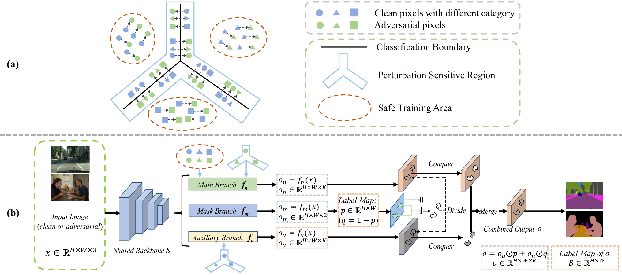
DDC-AT adopts a divide-and-conquer procedure during training, as shown in Fig. 2 (b) and explained as the following. 1) Divide: for an input image , DDC-AT divides its pixels into two sub-tasks for two branches, respectively. 2) Conquer: each branch predicts labels for the pixels assigned to it. 3) Merge: predictions from two branches are merged into the final prediction of image .
Dividing pixels.
To improve the segmentation accuracy, previous work [26] has shown that we can divide pixels of one image into different kinds for individual processing, according to their property. As shown in Fig. 2(a), clean pixels in the output space can be divided into two types during training, according to their “boundary property”.
1) Pixels without “boundary property”: clean pixels and their paired adversarial pixels are in the same classification space (in the “Safe Training Area”). The properties of clean and adversarial pixels are similar in the output space. They are likely to stay far away from the boundary. Their distribution can be aligned in the same branch with adversarial training. The location of in is the set .
2) Pixels with “boundary property”: clean pixels and their paired adversarial pixels are in diverse classification spaces. Such clean pixels are likely to stay near the classification boundary (in the “Perturbation Sensitive Region”). They have “boundary property” since they are easy to perturb through the boundary. Directly aligning them with the adversarial pixels in the same branch is difficult, since their distributions differ widely. We propose to first use two different branches to train them respectively. Once the clean and their adversarial pixels stay in the same space, we align them in the same branch. Contrary to , the location of in is the set .
In short, we divide pixels in one clean image according to whether they have “boundary property” or not. The “boundary property” describes whether clean pixels and the corresponding adversarial pixels have different predictions or not. For semantic segmentation, normally not all pixels in a clean sample are perturbed to have wrong predictions after adding adversarial noise [46, 31, 1]. Thus, some pixels in a clean sample have the boundary property while others do not. Such division can be completed dynamically via training a “mask branch” that distinguishes among pixels with and without boundary property. Implementation of training will be discussed in Sec. 5.2.
Conquering pixels.
Based on above division setting, we set our framework as shown in Fig. 2(b), which consists of three branches. They are “main branch”, “auxiliary branch”, and “mask branch”, denoted as , and respectively. and can be utilized to conquer pixels, i.e., predicting labels for pixels assigned to them through forwarding the corresponding networks. We use “main branch” to conquer , as well as all adversarial pixels, and use “auxiliary branch” to conquer . In this way, clean pixels in one image after division are processed by different branches. In addition, and share the backbone. Thus they help each other in the feature level. It is noteworthy that only is used in inference.
Merging pixels.
As shown in Fig. 2(b), divided pixels after conquering are merged. This is because all pixels in one clean image are divided into and , and there is no overlap between the pixels assigned to and . Therefore, they can be merged into the final prediction of the input image to compute loss, according to the division. This also indicates that the output space to decide the division should be the combination of and during training.
Parameter: clean data with one-hot label , all-zero matrix 0, function ( if is True)
Parameter: clean training set , shared backbone , main branch , auxiliary branch , mask branch , training batch size , and maximum training iteration , the number of iterations
5.2 Dynamical Division and Implementation
In this section, we illustrate the dynamical property of division setting in DDC-AT, and explain how such division is achieved through training a “mask branch”.
Dynamical division.
Clean pixels belonging to are first used in the auxiliary branch for training. They become robust towards adversarial perturbations in and turn into . Then they move to the main branch . In this way, all clean pixels gradually move into .
In this design, the main branch finally trains all clean pixels, far away from the boundary. This mechanism effectively avoids drop of performance on clean samples. Moreover, training adversarial pixels with improves robustness towards adversarial perturbation for the main branch.
Implementation.
DDC-AT distributes all adversarial pixels into , and adopts dynamical division for clean pixels. Such division is implemented with a “mask branch” .
(a) Predicting . First, predicts pixels in the input image, as shown in Fig. 2(b). For an input , output from , , and is , , and respectively. The label map of is , which is a binary matrix to decide division. means pixel belongs to and is sent to . Otherwise, it moves to . This operation yields the combined output for as , as shown in Fig. 2(b). Here is the Hadamard product. If is perturbed to , we denote the combined output as and , which are obtained in the same way.
(b) Ground truth. Next, the ideal division scheme is based on the combined output. This scheme has a “mask label” notation . means the pixel in location belongs to and is “divided into ”. Otherwise, it is “divided into ”. We set the mask label for as , and denote the label map of and as and respectively. For pixel , if , it sets into since it has the boundary property. In this case, we set . Otherwise, it sends to , making . Besides, all adversarial pixels should be sent to , and we set mask label for as , which is the matrix with all elements being zero.
(c) Training. and are obtained according to the ideal division rule in DDC-AT. We use them as the ground truth to train . Repeating the whole process makes learn how to achieve ideal division for pixels automatically. The algorithm to obtain and is summarized in Alg. 2. Note that learning of does not need external supervised information.
(d) Results. turns to and is assigned into progressively during training. This process is explained in Sec. 6.6. Finally, almost all pixels are assigned into , the decision boundary of tightly approaches that of the overall framework, and the predicted mask has almost all zero values.
5.3 Overall Loss Function
For the training data ( or ), its label map obtained from the mask branch is , and we set . The loss of for and is written as
| (3) |
where is the operation to compute the mean value, is the function of computing logarithm, , and are score maps with shape . Turning the mask label for into one-hot form , the loss for becomes
| (4) |
Combined with Eqs. (3) and (4), the overall loss term is
| (5) |
where , , and are set to 1 in experiments. Overall training procedure is concluded in Alg. 3.
5.4 Superiority of Divide-and-Conquer
DDC-AT is superior to SAT, proved in our experiments. It yields much better performance than classical SAT on both clean and adversarial pixels. We explain it below.
1) For segmentation, usually not all pixels in a clean sample are perturbed to have wrong predictions after adding adversarial noise. Some pixels have boundary property while others do not, and mask branch divides pixels into and based on their boundary properties. This motivates our division strategy.
2) First, for the training of clean pixels in the main branch , training with only (setting of DDC-AT) is much easier than mixed training with both and (setting of SAT). The introduced auxiliary branch in DDC-AT can turn into gradually and effectively. Thus, the main branch that is adopted for inference can better handle clean pixels and improve accuracy over SAT.
3) Second, to obtain decent results on adversarial pixels, SAT trains adversarial pixels with both and , while DDC-AT trains adversarial pixels with only for the main branch . Obviously, training with both and causes higher difficulty for the learning of adversarial pixels than training with only. Thus, DDC-AT yields higher accuracy on adversarial pixels.
6 Experiments
The newly proposed SAT and DDC-AT are effective for robust semantic segmentation. We evaluate our method on challenging PASCAL VOC 2012 [13] and Cityscapes [9] datasets, with popular semantic segmentation architectures PSPNet [50] and DeepLabv3 [7]. In the following, we first show implementation details related to training strategy and hyper-parameters. Then we exhibit results on corresponding datasets. The baseline is the method with no defense.
6.1 Datasets
PASCAL VOC 2012 (with abbreviation as VOC) [13] focuses on object segmentation. It contains 20 object classes and one class for background, with 1,464, 1,499, and 1,456 images for training, validation, and testing, respectively. The training set is augmented to 10,582 images in [18], which is also adopted. The Cityscapes [9] dataset is collected for urban scene understanding with 19 categories. It contains high-quality pixel-level annotations with 2,975, 500, and 1,525 images for training, validation, and testing.
6.2 Implementation Details
We choose popular semantic segmentation architectures PSPNet [50] and DeepLabv3 [7] for experiments. We follow the hyper-parameters as suggested in [49] for all models. Both SAT and DDC-AT train networks with augmentation of adversarial samples.
We choose white-box BIM attacker (by constraint) [24] to generate adversarial samples during training. The maximum perturbation value is set to . The consideration is that perturbation can be visually noticed by human [1] with larger values. The attack step size and number of attack iterations are set as and for training respectively. We use the mean of class-wise intersection over union (mIoU) as our evaluation metric. The parameters , and are kept constant during training. For each training mini-batch, half of the input includes adversarial samples that are dynamically decided by current model states, resulting in variance of results. For both SAT and DDC-AT, we train for one more time and report the average results as well as their standard deviations.
|
|
 |
 |
 |
 |
 |
|
|
 |
 |
 |
 |
 |
|---|---|---|---|---|---|
| Image | Ground Truth | No Defense | SAT | DDC-AT |
6.3 PASCAL VOC 2012
White-box attack.
White-box attackers utilize the exact gradient information of the target model [2]. Specifically, for the evaluation, we consider untargeted BIM attack ( constraint, , ) with ranging from 1 to 7, untargeted DeepFool attack ( constraint, ) [32], untargeted C&W attack ( constraint, ) [6], and untargeted BIM attack ( constraint, =3, , ).
| clean | Model: PSPNet | ||||||
|---|---|---|---|---|---|---|---|
| 2 | 4 | 6 | DeepFool | C&W | BIM | ||
| No Defense | 76.9 | 18.9 | 7.8 | 5.4 | 40.3 | 3.3 | 15.7 |
| SAT (Mean) | 74.3 | 68.1 | 44.5 | 27.9 | 59.0 | 65.5 | 36.4 |
| DDC-AT (Mean) | 76.0 | 75.6 | 47.9 | 33.8 | 61.2 | 67.4 | 37.1 |
| SAT (Std) | 0.5 | 1.8 | 2.9 | 3.2 | 1.4 | 1.2 | 4.1 |
| DDC-AT (Std) | 0.1 | 0.5 | 2.2 | 4.0 | 1.1 | 1.1 | 1.8 |
| clean | Model: DeepLabv3 | ||||||
| 2 | 4 | 6 | DeepFool | C&W | BIM | ||
| No Defense | 77.5 | 19.6 | 8.1 | 5.5 | 39.3 | 3.9 | 16.7 |
| SAT (Mean) | 72.7 | 62.4 | 43.1 | 28.8 | 59.0 | 66.0 | 37.0 |
| DDC-AT(Mean) | 75.2 | 69.9 | 43.6 | 32.3 | 60.4 | 67.1 | 37.8 |
| SAT (Std) | 1.0 | 0.6 | 1.9 | 2.0 | 0.4 | 1.2 | 1.1 |
| DDC-AT (Std) | 0.1 | 1.3 | 0.5 | 1.2 | 0.4 | 0.4 | 0.1 |
Results of different defense methods on VOC are shown in Table 1. We compare our methods with the baseline (model trained with clean samples only, without defense). All untargeted attacks yield a sharp performance drop without defense. Especially, under untargeted BIM attack ( constraint), the results approach zeros when the attack iteration number is large.
For BIM attack ( constraint), Table 1 basically indicates that results on adversarial samples with large attack iteration numbers represent the lower bound of each method on adversarial perturbation, since the corresponding performance decreases with the increase of , and converges when is large. Actually, the mean value of mIoU does not change more than 2.5% when is 10 or 20, compared with the results when =6 for No Defense, SAT and DDC-AT. This leads to the conclusion that SAT is already reasonable: it improves results from 5.4% to 27.9% on PSPNet and 5.5% to 28.8% on DeepLabv3 when . Moreover, SAT also improves results on other different types of attacks. Further, the standard deviation of SAT is low.
DDC-AT in Table 1 gives results of our final framework. Performance of DDC-AT on clean samples increases compared with SAT (by 1.7% and 2.5% on PSPNet and DeepLabv3, respectively), consistent with our design motivation. Further, the performance of DDC-AT is higher than SAT notably under each attacker iteration on average for BIM attack ( constraint). Intriguingly, the best case of SAT under every attack iteration is almost the worst case of DDC-AT. For example, when the attack iteration , we have on PSPNet and on DeepLabv3. More interestingly, for unseen attacks, DDC-AT also clearly improves robustness over SAT. The small standard deviation for DDC-AT indicates that results are stable. We also provide the visual comparison on VOC in Fig. 3 for comparing result quality.
| clean | Model: PSPNet | ||||||
|---|---|---|---|---|---|---|---|
| 2 | 4 | 6 | DeepFool | C&W | BIM | ||
| No Defense | 76.9 | 24.0 | 10.6 | 6.0 | 46.6 | 15.6 | 20.9 |
| SAT (Mean) | 74.3 | 56.5 | 51.3 | 44.9 | 64.0 | 68.5 | 58.7 |
| DDC-AT (Mean) | 76.0 | 61.5 | 53.4 | 46.1 | 68.4 | 70.5 | 59.6 |
| SAT (Std) | 0.5 | 2.9 | 2.8 | 4.2 | 2.1 | 1.3 | 3.0 |
| DDC-AT (Std) | 0.1 | 1.7 | 1.8 | 3.9 | 0.3 | 0.1 | 0.8 |
| clean | Model: DeepLabv3 | ||||||
| 2 | 4 | 6 | DeepFool | C&W | BIM | ||
| No Defense | 77.5 | 24.6 | 10.5 | 7.0 | 49.1 | 19.6 | 20.9 |
| SAT (Mean) | 72.7 | 51.8 | 51.0 | 45.0 | 64.4 | 68.5 | 64.5 |
| DDC-AT (Mean) | 75.2 | 60.4 | 52.6 | 46.0 | 68.7 | 70.6 | 65.9 |
| SAT (Std) | 1.0 | 3.8 | 3.7 | 4.1 | 1.8 | 1.6 | 0.4 |
| DDC-AT (Std) | 0.1 | 5.1 | 1.8 | 1.6 | 1.0 | 0.5 | 1.0 |
Black-box attack.
Black-box attackers cannot utilize the exact gradient information of the target model. Instead, gradient information from a substitute network, which is defensively trained on the same dataset [34, 33, 27], can be adopted. In our evaluation setting, the perturbation for trained PSPNet models is generated by DeepLabv3, trained on the same dataset and enhanced with adversarial training, and vice versa. For SAT and DDC-AT, the substitute networks are the same. As described in Sec. 6.2, models trained with the same method and dataset may demonstrate diverse behavior.
To reduce evaluation bias from training randomness, we evaluate SAT and DDC-AT on dataset in the following way. Using training strategy (SAT or DDC-AT) with a model structure on , we obtain model set . Then using adversarial training with a model structure different from on , we obtain model set as substitute defensive networks. Finally, for each model in , we use attack generated from each model in for evaluation.
The results under black-box evaluation on VOC are included in Table 2. The performance of clean models also decreases along with the increase of attack iteration for BIM attack ( constraint), like the white-box situation. This phenomenon suggests that there is strong transferability for adversarial samples in the semantic segmentation task. Therefore, it is meaningful to evaluate robustness under this black-box setting.
In comparison between DDC-AT and SAT, we use the same hyper-parameters as white-box attacks. From Table 2, it is clear that SAT also improves the defense effect under black-box attacks. The standard deviation of SAT is larger than the results by white-box attacks because black-box perturbation for each model is obtained from a set of substitute networks, which yield different adversarial behaviors.
The final performance of DDC-AT is consistently higher than SAT for BIM attack ( constraint) as well as other attacks. Meanwhile, standard deviations of DDC-AT are lower in all cases than SAT, especially under unseen attacks. It proves that DDC-AT is more stable than SAT by all types of attack.
| Model: PSPNet | Model: DeepLabv3 | |||||||
|---|---|---|---|---|---|---|---|---|
| clean | 2 | 4 | 6 | clean | 2 | 4 | 6 | |
| SAT (Mean) | 74.3 | 68.1 | 44.5 | 27.9 | 72.7 | 62.4 | 43.1 | 28.8 |
| DDC-AT-M (Mean) | 75.1 | 69.0 | 44.1 | 30.4 | 74.1 | 72.0 | 45.1 | 31.4 |
| DDC-AT-N (Mean) | 74.8 | 73.7 | 45.6 | 31.8 | 74.1 | 68.3 | 42.6 | 31.2 |
| DDC-AT (Mean) | 76.0 | 75.6 | 47.9 | 33.8 | 75.2 | 69.9 | 43.6 | 32.3 |
| SAT (Std) | 0.5 | 1.8 | 2.9 | 3.2 | 1.0 | 0.6 | 1.9 | 2.0 |
| DDC-AT-M (Std) | 0.1 | 3.1 | 0.9 | 4.0 | 0.1 | 4.6 | 4.7 | 3.8 |
| DDC-AT-N (Std) | 0.3 | 0.3 | 0.3 | 3.4 | 0.1 | 4.4 | 2.4 | 1.7 |
| DDC-AT (Std) | 0.1 | 0.5 | 2.2 | 4.0 | 0.1 | 1.3 | 0.5 | 1.2 |
6.4 Ablation Study
The motivation of DDC-AT is to dynamically divide pixels with/without boundary property into diverse branches during training. We prove our division setting is better than other alternatives by adjusting the division setting for pixels with boundary property. The alternatives are the following.
1) Use the “main branch” to deal with pixels from clean and adversarial samples without boundary property. Use “auxiliary branch” to process pixels from clean and adversarial samples with boundary property. We name this setting as DDC-AT-M.
2) Use the “main branch” to deal with pixels from clean samples, pixels from adversarial samples without boundary property. Use “auxiliary branch” to solve pixels from adversarial samples with boundary property. We name this setting as DDC-AT-N.
3)Use only the “main branch” to deal with pixels from either clean or adversarial samples. This is what SAT does, thus we do not train the mask branch.
For all these methods, only the main branch is utilized during testing. We evaluate the performances of these alternatives and list results in Table 3. For PSPNet model, the performance of DDC-AT-N is higher than SAT and lower than DDC-AT. Their standard deviations are in the same scale. The average results of DDC-AT-M are comparable with SAT and are worse than DDC-AT. Also, compared with DDC-AT, the standard deviation increases clearly by DDC-AT-M. This is because the adversarial samples during the training are different at every training iteration, and the dynamical distribution enhances such randomness. Similarly, for DeepLabv3 model, the average results of DDC-AT-M and DDC-AT-N are lower than DDC-AT, and higher than SAT consistently. The standard deviation increases compared with DDC-AT and SAT. In summary, the division setting of DDC-AT is optimal among these alternatives in terms of average performance and stability measurement.
| clean | Model: PSPNet | ||||||
|---|---|---|---|---|---|---|---|
| 2 | 4 | 6 | DeepFool | C&W | BIM | ||
| No Defense | 74.6 | 26.2 | 5.5 | 2.1 | 35.8 | 13.8 | 22.7 |
| SAT (Mean) | 69.0 | 46.7 | 32.9 | 25.8 | 56.0 | 49.1 | 45.8 |
| DDC-AT (Mean) | 71.7 | 50.2 | 34.7 | 28.7 | 57.2 | 50.8 | 46.7 |
| SAT (Std) | 1.0 | 1.0 | 0.3 | 1.0 | 3.0 | 1.5 | 1.8 |
| DDC-AT (Std) | 0.1 | 0.2 | 0.2 | 0.3 | 0.1 | 0.1 | 0.1 |
| clean | Model: DeepLabv3 | ||||||
| 2 | 4 | 6 | DeepFool | C&W | BIM | ||
| No Defense | 74.8 | 26.0 | 5.7 | 2.3 | 31.5 | 13.8 | 22.6 |
| SAT (Mean) | 69.4 | 46.1 | 31.8 | 26.2 | 56.7 | 48.4 | 45.0 |
| DDC-AT (Mean) | 71.3 | 50.9 | 34.9 | 29.0 | 57.4 | 50.5 | 46.8 |
| SAT (Std) | 1.0 | 1.0 | 0.6 | 0.4 | 1.7 | 1.3 | 0.9 |
| DDC-AT (Std) | 0.3 | 0.4 | 0.2 | 0.2 | 0.2 | 1.5 | 0.4 |
| clean | Model: PSPNet | ||||||
|---|---|---|---|---|---|---|---|
| 2 | 4 | 6 | DeepFool | C&W | BIM | ||
| No Defense | 74.6 | 28.0 | 6.9 | 3.3 | 35.6 | 21.1 | 25.3 |
| SAT (Mean) | 69.0 | 44.4 | 36.7 | 30.8 | 57.7 | 57.8 | 56.6 |
| DDC-AT (Mean) | 71.7 | 50.6 | 37.9 | 32.3 | 58.6 | 58.4 | 57.4 |
| SAT (Std) | 1.0 | 3.0 | 3.3 | 2.6 | 2.4 | 2.0 | 2.5 |
| DDC-AT (Std) | 0.1 | 1.0 | 1.0 | 0.2 | 0.1 | 0.1 | 0.3 |
| clean | Model: DeepLabv3 | ||||||
| 2 | 4 | 6 | DeepFool | C&W | BIM | ||
| No Defense | 74.8 | 29.9 | 7.6 | 3.1 | 35.8 | 27.3 | 27.3 |
| SAT (Mean) | 69.4 | 43.2 | 36.1 | 31.6 | 58.4 | 58.3 | 57.4 |
| DDC-AT (Mean) | 71.3 | 47.8 | 37.8 | 32.8 | 59.6 | 59.7 | 59.2 |
| SAT (Std) | 1.0 | 3.0 | 3.0 | 2.3 | 1.1 | 1.8 | 2.3 |
| DDC-AT (Std) | 0.3 | 1.9 | 1.0 | 0.3 | 0.7 | 0.5 | 0.2 |
| PSPNet (white-box) | PSPNet (black-box) | |||||||
|---|---|---|---|---|---|---|---|---|
| 2 | DeepFool | C&W | BIM | 2 | DeepFool | C&W | BIM | |
| multi-task [23] | 38.4 | 40.6 | 26.3 | 34.2 | 40.1 | 42.4 | 28.6 | 35.5 |
| multi-task [30] | 30.3 | 37.6 | 17.3 | 25.8 | 31.4 | 38.2 | 23.6 | 27.3 |
| TS [3] | 41.6 | 54.3 | 40.4 | 43.8 | 43.2 | 55.7 | 42.6 | 49.2 |
| TS [4] | 47.9 | 56.8 | 44.5 | 45.2 | 48.3 | 57.1 | 47.2 | 51.8 |
| DDC-AT | 50.2 | 57.2 | 50.8 | 46.7 | 50.6 | 58.6 | 58.4 | 57.4 |
| DeepLabv3 (white-box) | DeepLabv3 (black-box) | |||||||
| 2 | DeepFool | C&W | BIM | 2 | DeepFool | C&W | BIM | |
| multi-task [23] | 37.5 | 41.2 | 27.4 | 35.8 | 41.6 | 44.1 | 32.3 | 37.9 |
| multi-task [30] | 28.9 | 35.3 | 16.8 | 25.5 | 31.8 | 38.7 | 30.2 | 31.4 |
| TS [3] | 42.3 | 54.0 | 41.1 | 42.4 | 44.5 | 56.2 | 44.8 | 51.5 |
| TS [4] | 48.1 | 55.3 | 46.5 | 45.3 | 50.3 | 57.6 | 50.3 | 53.7 |
| DDC-AT | 50.9 | 57.4 | 50.5 | 46.8 | 47.8 | 59.6 | 59.7 | 59.2 |
6.5 Cityscapes
White-box attack.
The results of different methods on clean samples are included in Table 4. DDC-AT effectively reduces the drop of performance on clean samples, compared with SAT. DDC-AT improves mIoU on clean samples by 2.7% and 1.9%, which are significant with the setting of PSPNet and DeepLabv3, compared with SAT. The results of DDC-AT are also more stable over SAT.
We show results under white-box attack on Cityscapes dataset in Table 4. Obviously, clean models get worse with the increase of attack iterations for BIM attack ( constraint), like the case in VOC, which proves the general effect of the adversarial attack on different datasets. The results of DDC-AT and SAT under various attack iterations for BIM attack ( constraint) are like we observe before – they also improve the robustness of the models on this large dataset.
DDC-AT outperforms SAT in Table 4 where the best cases of SAT under every attack iteration are actually worse than the worst cases of DDC-AT. Further, DDC-AT also outperforms SAT on other types of attacks in this dataset. As shown in Table 4, both DDC-AT and SAT are stable, while DDC-AT is even better.
Black-box attack.
The results under the evaluation of the black-box attack for the Cityscapes dataset are shown in Table 5. DDC-AT also outperforms SAT on average with various types of attacks. The standard deviation of DDC-AT is still strictly smaller than that of SAT. For example, when , the standard deviation of SAT is larger than 2% for both PSPNet and DeepLabv3, while the standard deviation of DDC-AT is smaller than 0.5%. Our method also outperforms [23, 30, 3, 4] as shown in Table 6.
6.6 The Output of
As we have mentioned, clean pixels with the boundary property () are first set to for training, and they will gradually be turned into clean pixels without the boundary property (). The number of the predicted in one clean image is decided by the output of , i.e., the total number of non-zero values in the label map , as clarified in Sec. 5.2. And the number of the real can be computed as the total number of non-zero values in the mask label , as clarified in Sec. 5.2 and Alg. 2. We display the average proportion of the predicted/real in one clean image with respect to the number of training epoch in Fig. 4. Obviously, the proportion of the predicted and real gradually approaches zeros. The tendency of the predicted follows the real , since the mask branch is supervised by the mask label , as shown in Eq. (4). All these results show that gradually turns into .
7 Conclusion
In this paper, we have explored the property of adversarial training on the semantic segmentation task. Our defense strategy can consistently enhance the robustness of target models under adversarial attacks. Besides proposing the standard adversarial training (SAT) process, we propose a new strategy to improve the performance of adversarial training in this task, with no extra parameter and computation cost introduced during inference. The extensive experimental results with different model structures on two representative benchmark datasets suggest that the proposed method achieves significantly better generalization and stability on unseen adversarial examples and clean samples, compared with standard adversarial training.
References
- [1] Anurag Arnab, Ondrej Miksik, and Philip HS Torr. On the robustness of semantic segmentation models to adversarial attacks. In CVPR, 2018.
- [2] Anish Athalye and Nicholas Carlini. On the robustness of the cvpr 2018 white-box adversarial example defenses. arXiv:1804.03286, 2018.
- [3] Andreas Bar, Fabian Huger, Peter Schlicht, and Tim Fingscheidt. On the robustness of redundant teacher-student frameworks for semantic segmentation. In CVPRW, 2019.
- [4] Andreas Bar, Marvin Klingner, Serin Varghese, Fabian Huger, Peter Schlicht, and Tim Fingscheidt. Robust semantic segmentation by redundant networks with a layer-specific loss contribution and majority vote. In CVPRW, 2020.
- [5] Qi-Zhi Cai, Min Du, Chang Liu, and Dawn Song. Curriculum adversarial training. IJCAI, 2018.
- [6] Nicholas Carlini and David Wagner. Towards evaluating the robustness of neural networks. In IEEE symposium on security and privacy, 2017.
- [7] Liang-Chieh Chen, George Papandreou, Florian Schroff, and Hartwig Adam. Rethinking atrous convolution for semantic image segmentation. arXiv:1706.05587, 2017.
- [8] Moustapha Cisse, Piotr Bojanowski, Edouard Grave, Yann Dauphin, and Nicolas Usunier. Parseval networks: Improving robustness to adversarial examples. In ICML, 2017.
- [9] Marius Cordts, Mohamed Omran, Sebastian Ramos, Timo Rehfeld, Markus Enzweiler, Rodrigo Benenson, Uwe Franke, Stefan Roth, and Bernt Schiele. The cityscapes dataset for semantic urban scene understanding. In CVPR, 2016.
- [10] Guneet S Dhillon, Kamyar Azizzadenesheli, Zachary C Lipton, Jeremy Bernstein, Jean Kossaifi, Aran Khanna, and Anima Anandkumar. Stochastic activation pruning for robust adversarial defense. In ICLR, 2018.
- [11] Yifan Ding, Liqiang Wang, Huan Zhang, Jinfeng Yi, Deliang Fan, and Boqing Gong. Defending against adversarial attacks using random forest. In CVPRW, 2019.
- [12] Yinpeng Dong, Fangzhou Liao, Tianyu Pang, Hang Su, Jun Zhu, Xiaolin Hu, and Jianguo Li. Boosting adversarial attacks with momentum. In CVPR, 2018.
- [13] Mark Everingham, Luc Van Gool, Christopher KI Williams, John Winn, and Andrew Zisserman. The pascal visual object classes (voc) challenge. IJCV, 2010.
- [14] Ian Goodfellow, Jean Pouget-Abadie, and Mehdi Mirza. Generative adversarial nets. In NIPS, 2014.
- [15] Ian J Goodfellow, Jonathon Shlens, and Christian Szegedy. Explaining and harnessing adversarial examples. ICLR, 2014.
- [16] Shixiang Gu and Luca Rigazio. Towards deep neural network architectures robust to adversarial examples. arXiv:1412.5068, 2014.
- [17] Chuan Guo, Mayank Rana, Moustapha Cisse, and Laurens Van Der Maaten. Countering adversarial images using input transformations. In ICLR, 2018.
- [18] Bharath Hariharan, Pablo Arbeláez, Ross Girshick, and Jitendra Malik. Hypercolumns for object segmentation and fine-grained localization. In CVPR, 2015.
- [19] Wei-Chih Hung, Yi-Hsuan Tsai, and Yan-Ting Liou. Adversarial learning for semi-supervised semantic segmentation. In BMVC, 2018.
- [20] Nathan Inkawhich, Wei Wen, Hai Helen Li, and Yiran Chen. Feature space perturbations yield more transferable adversarial examples. In CVPR, 2019.
- [21] Xiaojun Jia, Xingxing Wei, Xiaochun Cao, and Hassan Foroosh. Comdefend: An efficient image compression model to defend adversarial examples. In CVPR, 2019.
- [22] Harini Kannan, Alexey Kurakin, and Ian Goodfellow. Adversarial logit pairing. arXiv:1803.06373, 2018.
- [23] Marvin Klingner, Andreas Bar, and Tim Fingscheidt. Improved noise and attack robustness for semantic segmentation by using multi-task training with self-supervised depth estimation. In CVPRW, 2020.
- [24] Alexey Kurakin, Ian Goodfellow, and Samy Bengio. Adversarial examples in the physical world. ICLR, 2016.
- [25] Alexey Kurakin, Ian Goodfellow, and Samy Bengio. Adversarial machine learning at scale. ICLR, 2016.
- [26] Xiaoxiao Li, Ziwei Liu, Ping Luo, Chen Change Loy, and Xiaoou Tang. Not all pixels are equal: Difficulty-aware semantic segmentation via deep layer cascade. In CVPR, 2017.
- [27] Yanpei Liu, Xinyun Chen, Chang Liu, and Dawn Song. Delving into transferable adversarial examples and black-box attacks. In ICLR, 2017.
- [28] Pauline Luc, Camille Couprie, and Soumith Chintala. Semantic segmentation using adversarial networks. arXiv:1611.08408, 2016.
- [29] Aleksander Madry, Aleksandar Makelov, Ludwig Schmidt, Dimitris Tsipras, and Adrian Vladu. Towards deep learning models resistant to adversarial attacks. In ICLR, 2018.
- [30] Chengzhi Mao, Amogh Gupta, Vikram Nitin, Baishakhi Ray, Shuran Song, Junfeng Yang, and Carl Vondrick. Multitask learning strengthens adversarial robustness. ECCV, 2020.
- [31] Jan Hendrik Metzen, Mummadi Chaithanya Kumar, Thomas Brox, and Volker Fischer. Universal adversarial perturbations against semantic image segmentation. In ICCV, 2017.
- [32] Seyed-Mohsen Moosavi-Dezfooli, Alhussein Fawzi, and Pascal Frossard. Deepfool: a simple and accurate method to fool deep neural networks. In CVPR, 2016.
- [33] Nicolas Papernot, Patrick McDaniel, and Ian Goodfellow. Transferability in machine learning: from phenomena to black-box attacks using adversarial samples. arXiv:1605.07277, 2016.
- [34] Nicolas Papernot, Patrick McDaniel, Ian Goodfellow, Somesh Jha, Z Berkay Celik, and Ananthram Swami. Practical black-box attacks against machine learning. In ACM on Asia conference on computer and communications security, 2017.
- [35] Nicolas Papernot, Patrick McDaniel, Somesh Jha, Matt Fredrikson, Z Berkay Celik, and Ananthram Swami. The limitations of deep learning in adversarial settings. In 2016 IEEE European Symposium on Security and Privacy, 2016.
- [36] Aaditya Prakash, Nick Moran, Solomon Garber, Antonella DiLillo, and James Storer. Deflecting adversarial attacks with pixel deflection. In CVPR, 2018.
- [37] Edward Raff, Jared Sylvester, Steven Forsyth, and Mark McLean. Barrage of random transforms for adversarially robust defense. In CVPR, 2019.
- [38] Chuanbiao Song, Kun He, Liwei Wang, and John E Hopcroft. Improving the generalization of adversarial training with domain adaptation. ICLR, 2018.
- [39] Yang Song, Taesup Kim, Sebastian Nowozin, Stefano Ermon, and Nate Kushman. Pixeldefend: Leveraging generative models to understand and defend against adversarial examples. In ICLR, 2018.
- [40] Christian Szegedy, Wojciech Zaremba, Ilya Sutskever, Joan Bruna, Dumitru Erhan, Ian Goodfellow, and Rob Fergus. Intriguing properties of neural networks. arXiv:1312.6199, 2013.
- [41] Florian Tramèr, Alexey Kurakin, Nicolas Papernot, Ian Goodfellow, Dan Boneh, and Patrick McDaniel. Ensemble adversarial training: Attacks and defenses. ICLR, 2017.
- [42] Jianyu Wang and Haichao Zhang. Bilateral adversarial training: Towards fast training of more robust models against adversarial attacks. In ICCV, 2019.
- [43] Weibin Wu, Yuxin Su, Xixian Chen, Shenglin Zhao, Irwin King, Michael R Lyu, and Yu-Wing Tai. Boosting the transferability of adversarial samples via attention. In CVPR, 2020.
- [44] Chaowei Xiao, Ruizhi Deng, Bo Li, Fisher Yu, Mingyan Liu, and Dawn Song. Characterizing adversarial examples based on spatial consistency information for semantic segmentation. In ECCV, 2018.
- [45] Cihang Xie, Jianyu Wang, Zhishuai Zhang, Zhou Ren, and Alan Yuille. Mitigating adversarial effects through randomization. ICLR, 2017.
- [46] Cihang Xie, Jianyu Wang, Zhishuai Zhang, Yuyin Zhou, Lingxi Xie, and Alan Yuille. Adversarial examples for semantic segmentation and object detection. In CVPR, 2017.
- [47] Cihang Xie, Yuxin Wu, Laurens van der Maaten, Alan L Yuille, and Kaiming He. Feature denoising for improving adversarial robustness. In CVPR, 2019.
- [48] Haichao Zhang and Jianyu Wang. Defense against adversarial attacks using feature scattering-based adversarial training. In NIPS, 2019.
- [49] Hengshuang Zhao. semseg. https://github.com/hszhao/semseg, 2019.
- [50] Hengshuang Zhao, Jianping Shi, Xiaojuan Qi, Xiaogang Wang, and Jiaya Jia. Pyramid scene parsing network. In CVPR, 2017.