A Persistent Homology Approach to Time Series Classification
Abstract
Topological Data Analysis (TDA) is a rising field of computational topology in which the topological structure of a data set can be observed by persistent homology. By considering a sequence of sublevel sets, one obtains a filtration that tracks changes in topological information. These changes can be recorded in multi-sets known as persistence diagrams. Converting information stored in persistence diagrams into a form compatible with modern machine learning algorithms is a major vein of research in TDA. Persistence curves, a recently developed framework, provides a canonical and flexible way to encode the information presented in persistence diagrams into vectors. In this work, we propose a new set of metrics based on persistence curves. We prove the stability of the proposed metrics. Finally, we apply these metrics to the UCR Time Series Classification Archive. These empirical results show that our metrics perform better than the relevant benchmark in most cases and warrant further study.
1 Introduction
In recent years, Topological Data Analysis (TDA) has expanded rapidly. With applications in health research [12], 3D modeling [17], and aviation [13], the field is poised to become a staple of data analytics. Among the tools available to a topological data analyst is persistent homology. This tool considers a dataset at all scales simultaneously via sequence of topological spaces and tracks when topological features appear (are born) and disappear (die) within the sequence. These birth-death times can be collected and stored in a multi-set known as a persistence diagram; however, these diagrams are not compatible with modern machine and deep learning algorithms. This discrepancy has lead to several projects dedicated to summarizing persistence diagrams in such a way that preserves the topological information and is compatible with machine and deep learning. Summaries such as the persistence images [1], the persistence landscapes [4], and the persistent entropy [2]. The particular interest in this paper is the persistence curve framework [6]. In that work, they showed this framework capable of generating new summaries as well as several well-known summaries such as persistence landscapes and persistent entropy. Recently, there has been some work on applying TDA tools to classify time series. For instance, in these work [18], [19], and [16], authors used lag map method to reconstruct the attractors and utilized TDA tools (more precisely, the Rips complex filtration) to extract features from those attractors. In [14], authors defined a new distance on the space of persistence diagram and used this new distance to classify time series. In [20] and [5], authors used TDA tools to analyze physiological signals.
In this paper, our main contribution is to use persistence curves to define two ensemble metrics for the difference of two time series. One of the ensemble metrics uses the Euclidean 1-norm while the other uses the Dynamic Time Warping (DTW) Distance between time series introduced in [3]. In Section 2, we provide a gentle introduction to persistent homology and persistence curves and explain how we extract these objects from time series. In Section 3, we introduce the topological transformation of a time series, and the definition of our proposed metrics is presented in Section 4. Finally, in Section 5, we apply these new distances to the UCR Time Series archive [8] via a 1-NN test and compare our results to the reported benchmark in the database.
2 Mathematical Background
We will lay out the basic mathematical concepts to equip the reader with the tools to understand the models developed later. We begin by discussing time series and Dynamic Time Warping before moving on to homology, persistent homology, and persistence curves.
2.1 Time Series and Dynamic Time Warping
For a natural number let . A time series is a function . We commonly write for . Given a time series we can produce a continuous piecewise linear functional representation of by linearly interpolating between the points of . One can show in this setting that the 1-norm of a time series bounds the 1-norm of its functional representation from above and similarly for the -norm. That is and where . Moreover, we have . Note these inequalities are achievable due to the fact that is continuous, bounded, and defined on a compact domain. To prove that the discrete 1-norm is larger than the continuous 1-norm suppose we have a non-negative time series . The corresponding piecewise linear function is . Integrating this function from to gives ; however, . Consider . The area under the corresponding piecewise linear curve is given by . But this is exactly . So if is any time series with corresponding function then one may consider the time series where . This is a nonnegative time series whose corresponding function is exactly defined by . Moreover, and . The previous argument applies and we see
We will now discuss Dynamic Time Warping [3]. For the rest of this section, let and be time series defined on and respectively. A warping path between and is a function so that and , where is the length of the path from to . We denote the collection of warping path between and by . A warping path induces two time series and both defined on where and , where is the projection to the -th coordinate for .
Let be non-negative. The cost of a warping path between and can be defined as . In this paper, we choose . For instance, suppose , and consider the “diagonal” path . Then
The Dynamic Time Warping distance (DTW distance) between and is defined to be the minimum cost over all warping paths. That is,
| (1) |
There is a relation between DTW distance and Euclidean distance. Observe that since , one has
| (2) |
It is well known that the functional representations of any two time series - two 1-dimensional lines without loops - are homeomorphic, i.e. either one may be continuously morphed into the other without punctures or tears. Heuristically, one can view the DTW distance measure of cost for that morphing.
2.2 Persistent Homology
Homology is a classic subject in mathematics that provides information about a topological space that is invariant under continuous deformations. This means that the homology of a space gives us useful information about its topological structure. Informally, the -th homology group of a space is often used to count the -th Betti numbers, i.e. the number of -dimensional holes of . For example, counts the connected components and counts loops, counts voids or “air pockets”, and so on.
Persistent homology, first defined in [10] is a powerful tool from the field of topological data analysis that tracks the changes of homology over a filtration.
A filtration of a space is an increasing sequence of spaces . One may obtain homology groups for each . Because of the subset relations, we can track the changes of homology groups. This process is what we call persistent homology. For a time series with corresponding continuous piecewise linear function , we can obtain a filtration by considering sublevel sets . The inclusion induces a map between the homology groups. We note that homology in this sequence only changes at critical values of . [9]
We say a homology class is born at if we have and . We say that born at dies at , if , but , i.e. if it merges with a previous class. The ranks for form the persistent Betti numbers of the filtration.
These persistent Betti numbers count the number of classes that were born at or before and are still alive at . Inclusion-exclusion allows us to count exactly the number of classes born at and die at by . The -th persistence diagram, or just diagram, associated to the filtering function of a space is a multi-set, that is a set of points with multiplicity, of birth-death pairs with multiplicity along with the diagonal points each with infinite multiplicity. To shorten notation, we will often represent persistence diagrams with the letter .
The stability theorem for persistence diagrams, which first appeared in [7], states that if are functions that have finitely many critical values then
where is known as the Wasserstein -metric, or bottleneck distance defined as
where , .
This stability theorem tells us that if the original space is altered by a small amount, then the diagrams are altered by a small amount. Because diagrams are not readily compatible with machin learning, we need to summarize them in some way. In the next section, we will discuss the persistence curve framework, which is capable of generating summaries of diagrams.
2.3 Persistence Curves
Persistence Curves, first defined in [6], draws inspiration from the Fundamental Lemma of Persistent Homology, which states that the Betti number of an element in the filtration is given by . The statement here says that the -th Betti number of the subspace is given exactly by the number of points in the box formed by the points up and to the left of the diagonal at .
Persistence curves take this concept and generalize it. Instead of just counting the points, we will place a function over the points and compute some statistic over the aforementioned box. The idea is formalized follows.
Let be a diagram and let . Suppose is a real-valued function so that . Let be a statistic, or a function of multi-set. We can define a persistence curve as:
We refer to the set as a fundamental box at . Figure illustrates a fundamental box. As a quick example, if is the sum statistic and if when and otherwise, then produces the Betti number curve. That is to say .
Generally, one chooses to be a function that carries useful information about the diagram points. In this paper, we are interested in one particular curve called the stabilized life curve. If then with we define the stabilized life curve as . Figure 1 illustrates the workflow of beginning with a time series, then computing the diagram via sublevel sets before finally computing the stabilized life curve. The top three images constitute a toy example in which the birth and death coordinates are connected to the cooresponding time series points.
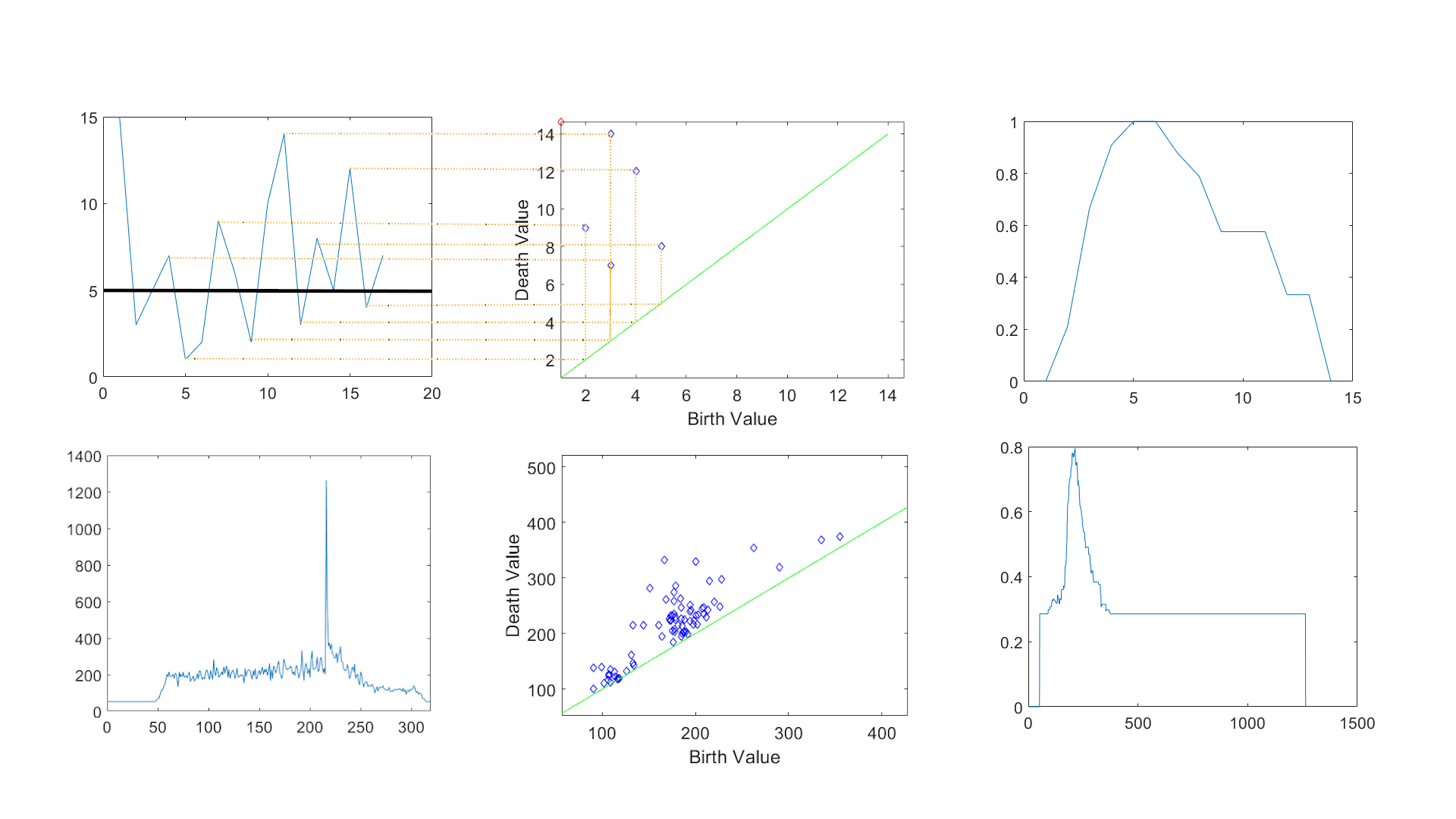
A general stability bound for persistence curves was established in [6], which we state below.
Theorem 1.
[6] Let be persistence diagrams. Let be the sum statistic. Suppose that . Let and be continuous functions. Then there exists a constant such that the following estimate holds
| (3) |
In essence, the constant depends on the function , and number of points in and . [6] provides an explicit form of . Since we will not use the its explicit form in this work, we refer interested readers to [6] for more details about the constant .
In practice, we need to discretize the persistence curves. Given a persistence curve and a mesh of points . The corresponding sequence is called a discretized persistence curve. As the number of points in the mesh increases, the discretized persistence curve approaches its continuous counterpart. Moreover, the proof of the stability for the continuous version can be altered to provide a proof for the same stability bound for the discretized curves, provided that the mesh contains all birth and death values of the diagram.
3 Topological Transformation of Time Series
Our main method transforms a time series into a set of persistence curves. This set of curves will be a topological representation of time series. The focus of this section is to show that such topological transformation is stable with a given metric. More precisely, a small perturbation in the original time series leads to a small change in the persistence curve. We prove stability results with two different metrics.
Let be a time series. We consider the usual continuous, piece-wise linear function representation of . We also consider a persistence diagrams of , , by sublevel set filtration. Lastly, we use a persistence curve to summarize . To ensure robustness, we provide a stability bound for the DTW distance on the discretized persistence curve. Prior to this, we show an interesting result bounding the bottleneck distance by the DTW distance.
Lemma 1.
Let be time series and suppose be their corresponding continuous piece-wise linear functions. Let be a mesh fine enough to contain all birth and death values of and . Then
Proof.
let be the optimal path satisfying DTW distance between and . Denote the induced time series by and , where is the length of the optimal path ,
and corresponding functions and . By the definition of a warping path, namely that we have that can change in either coordinate by at most one and it cannot decrease. The proof of this is extraordinarily tedious. How about some heuristic like: The critical values of occur exactly at values of the time series. Let be the height of a critical value that causes a change in the homology of the sublevel set filtration. Let be the smallest index for which and let be the largest index so that . Then either and or and . By definition of DTW, there is some for which . Moreover, because can only change the first coordinate by at most one, the closest indices below and above for which heights are difference from have heights and . That is to say that is the height of a critical value that changes homology in the sublevel set filtration. A similar argument shows that these critical values for are critical values of . Therefore, has the same critical points as hence . The same argument shows . From the definition of DTW distance, one has . Once we put it all together we have the following string of inequalities:
∎
This lemma, to the best of our knowledge, is the first result that connects persistence diagram of sublevel set filtration of 1D function and DTW. It would be interesting to investigate relation between optimal match in Bottleneck distance and warping path in DTW.
We are now ready to present our main result.
Theorem 2.
Let and be the sum statistic. Let be time series and suppose be their corresponding continuous piecewise linear functions. Let be a mesh fine enough to contain all birth and death values of and .
Proof.
When , the proof is the direct result of the general bound persistence curves and the stability result for the bottleneck distance on persistence diagrams [7]. Note that for any time series , satisfies this regularity condition due to it being continuous and having finitely many critical values, hence we benefit from the diagram stability theorem.
To see the case of , we first ease notation by writing for , for , for and for .
We summarize all relations among different metrics that we have discussed in this paper:


We conclude this section by showing an example of proposed topological transformation. Figure 2 shows two examples of the result when we use the stabilized life curve. We consider the “Trace” and “SmoothSubspace” dataset as shown in Figure 2(a) and (b) respectively. Each dataset consists of three different classes which are shown in the blue, orange, and green, respectively. Notice on the left of (a) which shows the original time series, two classes of time series (orange and green ones noticeably. Moreover, the members of each class seem to be a horizontal translation of the other members. On the right of (a), we see the result of the topological transformation. Observe that not only does the transformation separate the classes, but also fixes the translation. In (b), we see on the left the original and on the right the transformation. Unfortunately, after the transformation the overlap clearly becomes worse. These examples motivate us to consider both geometric and topological information, and support exploration of the ensemble metric that we propose in the next section.
4 New Metrics
Persistence curves encode topological information into a format that is compatible with machine learning algorithms. By utilizing the original space in combination with the topological transformation, we introduce an ensemble metric and define a new distance between time series. Let . Let be a discretized persistence curve. If and are time series with corresponding continuous functions and . Finally let and .
Define the distance between and to be
Note that if , then this is not a true metric of and since we cannot guarantee that implies . We can define a similar metric by using the DTW distance:
These hybrid distances take both topological and geometric information into account. This new set of metrics contains two parameters. The first parameter is the , persistence curves. One may choose based on their prior knowledge about the dataset. [6] provides a list of persistence curves. The other parameter, , is a weighting of the distance between the original time series and the distance between their topological transformations. Based on different datasets, we believe can be optimized. In this work, we use and and as demonstration.
5 Applications to Time Series Classification
The UCR Time Series Archive [8] contains 128 datasets of time series gathered by different means for different scenarios and contributed by several different people. each dataset varies in train/test size and time series length. The task for each of these datasets is classification, and each dataset has a different number of classes. Some of the datasets were z-normalized and others were not. In our analysis, we did not attempt to alter the original time series in any other way than what was necessary to compute the topological transformation. The archive has reported three different benchmark models: Euclidean 2-norm distance 1-NN, DTW distance with a learned warping window 1-NN and DTW distance with a warping window of size 100 plut 1-NN. The administrator of the archive recommends those who are proposing new distance measurements to also perform the 1-NN test to allow for a proper comparison between the metrics. We performed our analyses in Python 3.7.1. We use the Perseus [15] software to compute persistence diagrams. In particular we make use of the cubtop function of Perseus. To use Perseus, one must input positive integers. Thus, to compute persistence, we transformed the time series in the following way: given a time series , we fill missing values with 0 and then map to a new time series via the formula for . Then by feeding this new time series into Perseus, we obtain a persistence diagram. We also note that due to the transformation , we obtain a natural mesh to compute a discretized persistence curve via the PersistenceCurves python package [11]. Note that by design, this mesh captures all possible birth and death values of diagrams arising from this process. Once we obtain a diagram , we compute the stabilized life, . For each folder in the UCR time series database, we performed 1-NN classifications with the and .
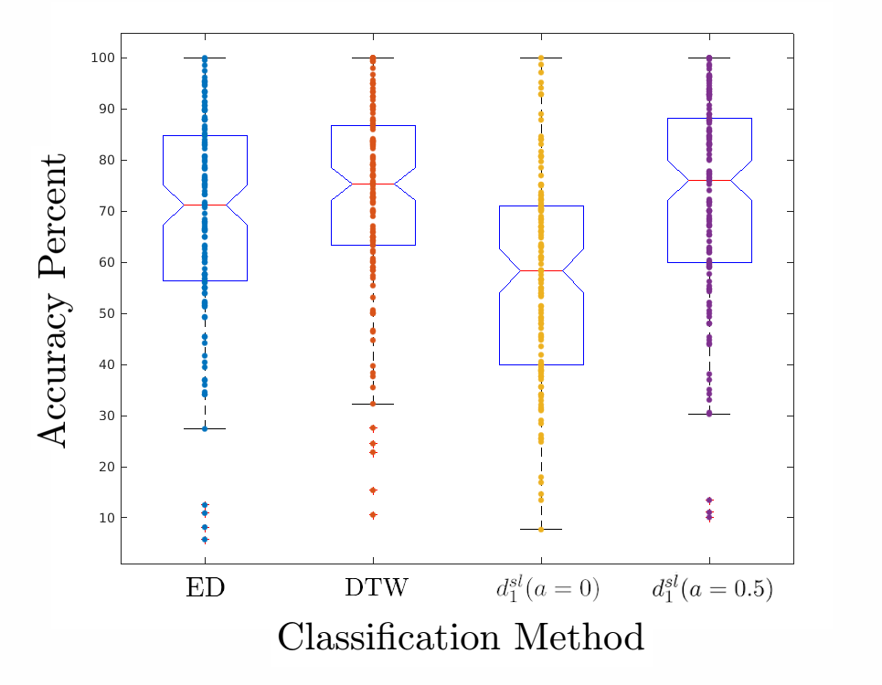
Figure 3 shows a boxplot of scores for each model considered. Notice that the as suggested in Section 3, the persistence curve alone does not perform well. We can see a comparison of each model and that the ensemble models perform well.
We moved on to testing the usefulness of these two metrics by measuring their performance on the UCR Time Series Archive via the 1-NN test. For the , we tested all 128 datasets in the archive. We found that the metric outperformed the reported Euclidean distance (ED) benchmark on the UCR Time Series by out of datasets as shown in Figure 4(a). Each plot in Figure 4 shows the difference in the accuracy scores between the given models for each of the UCR datasets in alphabetical order. For more details about performance of individual datasets, we include the Excel file of our main results in the supplementary file. A similarly good result came from weighting the topological features higher as shown in Figure 4(c).
If we compare this metric () to the UCR reported DTW (learned_w) benchmark, our results are better out of times and times for as shown in Figure 4(b) and (d).
The DTW ensemble metric was also tested on all UCR datasets. In these experiments, we did not make use of a warping window and instead calculated the DTW distance by using the full time series. Out of these 128 datasets, our results showed are better than DTW (learned_w) 61 times and tied 3 times.
When using , our results are better than the calculated DTW 64 times, tied 3 times. Figure 5 shows the differences in accuracy between the given models. We see the topological information is competitive with the learned warping window. It would be interesting to combine these two methods.


6 Conclusion
With the growing popularity of topological data analysis and computational topology as a whole, more researchers seek to understand data by studying it’s shape. In this work, we proposed a transformation of time series based on topology and in particular persistence curves. From here we proposed two families ensemble metrics that measures distance between two time series by considering the time series itself as well as their topological transforms and computes a weighted average of either the Euclidean or DTW distance on the respective parts. We provided a general stability result for the DTW distance as well as a concrete result for the stabilized life curve, which was the persistence curve we used in our experiments.
These initial results are promising and pave the way for future exploration through the addition of not only more datasets from the archive, but also for the inclusion of a warping window for DTW distance. Moreover, we focused only on the stabilized life curve in this work. The general nature of the persistence curve framework allows for a rich toolbox of curves to define or select from. With this in mind, we can ask the deeper question of curve selection. That is, given a dataset, is it possible to systematically decide, perhaps with a given family of persistence curves, which curve will perform optimally relative that family. On a broader level, we can ask to what extent can we develop a statistical/machine learning theory around this framework. These questions point to a multitude of research and application avenues in the future.
References
- [1] Henry Adams, Tegan Emerson, Michael Kirby, Rachel Neville, Chris Peterson, Patrick Shipman, Sofya Chepushtanova, Eric Hanson, Francis Motta, and Lori Ziegelmeier. Persistence images: A stable vector representation of persistent homology. The Journal of Machine Learning Research, 18(1):218–252, 2017.
- [2] N. Atienza, R. Gonzalez-Diaz, and M. Soriano-Trigueros. A new entropy based summary function for topological data analysis. Electronic Notes in Discrete Mathematics, 68:113 – 118, 2018. Discrete Mathematics Days 2018.
- [3] Donald J Berndt and James Clifford. Using dynamic time warping to find patterns in time series. In KDD workshop, volume 10, pages 359–370. Seattle, WA, 1994.
- [4] Peter Bubenik. Statistical topological data analysis using persistence landscapes. The Journal of Machine Learning Research, 16(1):77–102, 2015.
- [5] Yu-Min Chung, Chuan-Shen Hu, Yu-Lun Lo, and Hau-Tieng Wu. A persistent homology approach to heart rate variability analysis with an application to sleep-wake classification. arXiv preprint arXiv:1908.06856, 2019.
- [6] Yu-Min Chung and Austin Lawson. Persistence curves: A canonical framework for summarizing persistence diagrams, 2019.
- [7] David Cohen-Steiner, Herbert Edelsbrunner, and John Harer. Stability of persistence diagrams. Discrete & Computational Geometry, 37(1):103–120, 2007.
- [8] Hoang Anh Dau, Eamonn Keogh, Kaveh Kamgar, Chin-Chia Michael Yeh, Yan Zhu, Shaghayegh Gharghabi, Chotirat Ann Ratanamahatana, Yanping, Bing Hu, Nurjahan Begum, Anthony Bagnall, Abdullah Mueen, Gustavo Batista, and Hexagon-ML. The ucr time series classification archive, October 2018. https://www.cs.ucr.edu/~eamonn/time_series_data_2018/.
- [9] H. Edelsbrunner and J. Harer. Computational Topology: An Introduction. Miscellaneous Books. American Mathematical Society, 2010.
- [10] Herbert Edelsbrunner, David Letscher, and Afra Zomorodian. Topological persistence and simplification. In Proceedings 41st Annual Symposium on Foundations of Computer Science, pages 454–463. IEEE, 2000.
- [11] Austin Lawson. Persistencecurves. https://github.com/azlawson/PersistenceCurves.
- [12] Li Li, Wei-Yi Cheng, Benjamin S Glicksberg, Omri Gottesman, Ronald Tamler, Rong Chen, Erwin P Bottinger, and Joel T Dudley. Identification of type 2 diabetes subgroups through topological analysis of patient similarity. Science translational medicine, 7(311):311ra174–311ra174, 2015.
- [13] Max Z Li, Megan S Ryerson, and Hamsa Balakrishnan. Topological data analysis for aviation applications. Transportation Research Part E: Logistics and Transportation Review, 128:149–174, 2019.
- [14] Andrew Marchese and Vasileios Maroulas. Signal classification with a point process distance on the space of persistence diagrams. Advances in Data Analysis and Classification, 12(3):657–682, 2018.
- [15] Vidit Nanda. Perseus. http://www.sas.upenn.edu/~vnanda/perseus.
- [16] Lee M Seversky, Shelby Davis, and Matthew Berger. On time-series topological data analysis: New data and opportunities. In Proceedings of the IEEE Conference on Computer Vision and Pattern Recognition Workshops, pages 59–67, 2016.
- [17] Katharine Turner, Sayan Mukherjee, and Doug M. Boyer. Persistent homology transform for modeling shapes and surfaces. Information and Inference: A Journal of the IMA, 3(4):310–344, 12 2014.
- [18] Yuhei Umeda. Time series classification via topological data analysis. Information and Media Technologies, 12:228–239, 2017.
- [19] Vinay Venkataraman, Karthikeyan Natesan Ramamurthy, and Pavan Turaga. Persistent homology of attractors for action recognition. In 2016 IEEE international conference on image processing (ICIP), pages 4150–4154. IEEE, 2016.
- [20] Yuan Wang, Hernando Ombao, Moo K Chung, et al. Topological data analysis of single-trial electroencephalographic signals. The Annals of Applied Statistics, 12(3):1506–1534, 2018.