跳到论文正文
W Papers独立论文阅读器 arXiv:2003.06369 论文正文 计算阅读时间 · 0%
引用这篇论文根据当前论文元数据生成,正式投稿前建议核对。


License: arXiv.org perpetual non-exclusive license
arXiv:2003.06369v2 [math.OC] 23 Jun 2020

Boosting Frank-Wolfe by Chasing Gradients

Cyrille W. Combettes cyrille@gatech.edu
School of Industrial and Systems Engineering
Georgia Institute of Technology
Atlanta, GA, USA


Sebastian Pokutta pokutta@zib.de
Institute of Mathematics and Department for AI in Society, Science, and Technology
Technische Universität Berlin and Zuse Institute Berlin
Berlin, Germany

Abstract

The Frank-Wolfe algorithm has become a popular first-order optimization algorithm for it is simple and projection-free, and it has been successfully applied to a variety of real-world problems. Its main drawback however lies in its convergence rate, which can be excessively slow due to naive descent directions. We propose to speed up the Frank-Wolfe algorithm by better aligning the descent direction with that of the negative gradient via a subroutine. This subroutine chases the negative gradient direction in a matching pursuit-style while still preserving the projection-free property. Although the approach is reasonably natural, it produces very significant results. We derive convergence rates 𝒪⁡(1/t)\mathcal{O}(1/t) to 𝒪⁡(e−ω​t)\mathcal{O}(e^{-\omega t}) of our method and we demonstrate its competitive advantage both per iteration and in CPU time over the state-of-the-art in a series of computational experiments.

1 Introduction

Let (ℋ,⟨⋅,⋅⟩)(\mathcal{H},\langle\cdot,\cdot\rangle) be a Euclidean space. In this paper, we address the constrained convex optimization problem

minx∈𝒞⁡f⁡(x)\displaystyle\min_{x\in\mathcal{C}}f(x) (1)

where f:ℋ→ℝf:\mathcal{H}\rightarrow\mathbb{R} is a smooth convex function and 𝒞⊂ℋ\mathcal{C}\subset\mathcal{H} is a compact convex set. A natural approach to solving Problem (1) is to apply any efficient method that works in the unconstrained setting and add projections back onto 𝒞\mathcal{C} when the iterates leave the feasible region. However, there are situations where projections can be very expensive while linear minimizations over 𝒞\mathcal{C} are much cheaper. For example, if 𝒞={X∈ℝm×n∣‖X‖nuc⩽τ}\mathcal{C}=\{X\in\mathbb{R}^{m\times n}\mid\|X\|_{\operatorname{nuc}}\leqslant\tau\} is a nuclear norm-ball, a projection onto 𝒞\mathcal{C} requires computing an SVD, which has complexity 𝒪⁡(m​n​min⁡{m,n})\mathcal{O}(mn\min\{m,n\}), while a linear minimization over 𝒞\mathcal{C} requires only computing the pair of top singular vectors, which has complexity 𝒪⁡(nnz)\mathcal{O}(\operatorname{nnz}) where nnz\operatorname{nnz} denotes the number of nonzero entries. Other examples include the flow polytope, the Birkhoff polytope, the matroid polytope, or the set of rotations; see, e.g., Hazan and Kale 2012.

In these situations, the Frank-Wolfe algorithm (FW) (Frank and Wolfe 1956), a.k.a. conditional gradient algorithm (Levitin and Polyak 1966), becomes the method of choice, as it is a simple projection-free algorithm relying on a linear minimization oracle over 𝒞\mathcal{C}. At each iteration, it calls the oracle vt←arg​minv∈𝒞⁡⟨∇f​(xt),v⟩v_{t}\leftarrow\argmin_{v\in\mathcal{C}}\langle\nabla f(x_{t}),v\rangle and moves in the direction of this vertex, ensuring that the new iterate xt+1←xt+γt​(vt−xt)x_{t+1}\leftarrow x_{t}+\gamma_{t}(v_{t}-x_{t}) is feasible by convex combination, with a step-size γt∈[0,1]\gamma_{t}\in\left[0,1\right]. Hence, FW can be seen as a projection-free variant of projected gradient descent trading the gradient descent direction −∇f​(xt)-\nabla f(x_{t}) for the vertex direction vt−xtv_{t}-x_{t} minimizing the linear approximation of ff at xtx_{t} over 𝒞\mathcal{C}. FW has been applied to traffic assignment problems (LeBlanc et al. 1975), low-rank matrix approximation (Shalev-Shwartz et al. 2011), structural SVMs (Lacoste-Julien et al. 2013), video co-localization (Joulin et al. 2014), infinite RBMs (Ping et al. 2016), and, e.g., adversarial learning (Chen et al. 2020).

The main drawback of FW is that the modified descent direction leads to a sublinear convergence rate 𝒪⁡(1/t)\mathcal{O}(1/t), which cannot be improved upon in general as an asymptotic lower bound Ω⁡(1/t1+δ)\Omega(1/t^{1+\delta}) holds for any δ>0\delta>0 (Canon and Cullum 1968). More recently, Jaggi 2013 provided a simple illustration of the phenomenon: if f:x∈ℝn↦‖x‖22f:x\in\mathbb{R}^{n}\mapsto\|x\|_{2}^{2} is the squared ℓ2\ell_{2}-norm and 𝒞=Δn\mathcal{C}=\Delta_{n} is the standard simplex, then the primal gap at iteration t∈⟦1,n⟧t\in\llbracket 1,n\rrbracket is lower bounded by 1/t−1/n1/t-1/n; see also Lan 2013 for a lower bound Ω⁡(L​D2/t)\Omega(LD^{2}/t) on an equivalent setup, exhibiting an explicit dependence on the smoothness constant LL of ff and the diameter DD of 𝒞\mathcal{C}.

Hence, a vast literature has been devoted to the analysis of higher convergence rates of FW if additional assumptions on the properties of ff, the geometry of 𝒞\mathcal{C}, or the location of arg​min𝒞⁡f\argmin_{\mathcal{C}}f are met. Important contributions include:

  1. (i)

    𝒪⁡(e−ω​t)\mathcal{O}(e^{-\omega t}) if 𝒞\mathcal{C} is strongly convex and inf𝒞‖∇f‖>0\inf_{\mathcal{C}}\|\nabla f\|>0 (Levitin and Polyak 1966),

  2. (ii)

    𝒪⁡(e−ω​t)\mathcal{O}(e^{-\omega t}) if ff is strongly convex and arg​min𝒞⁡f⊂relint⁡(𝒞)\argmin_{\mathcal{C}}f\subset\operatorname{relint}(\mathcal{C}) (Guélat and Marcotte 1986),

  3. (iii)

    𝒪⁡(1/t2)\mathcal{O}(1/t^{2}) if ff is gradient dominated and 𝒞\mathcal{C} is strongly convex (Garber and Hazan 2015).

More recently, several variants to FW have been proposed, achieving linear convergence rates without excessively increasing the per-iteration complexity. These include the following:

  1. (i)

    𝒪⁡(e−ω​t)\mathcal{O}(e^{-\omega t}) when ff is strongly convex and 𝒞\mathcal{C} is a polytope (Garber and Hazan 2016; Lacoste-Julien and Jaggi 2015; Braun et al. 2019),

  2. (ii)

    𝒪⁡(e−ω​t)\mathcal{O}(e^{-\omega t}) with constants depending on the sparsity of the solution when ff is strongly convex and 𝒞\mathcal{C} is a polytope, of the form {x∈ℝn∣Ax=b,x⩾0}\{x\in\mathbb{R}^{n}\mid Ax=b,x\geqslant 0\} with vertices in {0,1}n\{0,1\}^{n} (Garber and Meshi 2016), or of arbitrary form (Bashiri and Zhang 2017).

Contributions.

We propose the Boosted Frank-Wolfe algorithm (BoostFW), a new and intuitive method speeding up the Frank-Wolfe algorithm by chasing the negative gradient direction −∇f​(xt)-\nabla f(x_{t}) via a matching pursuit-style subroutine, and moving in this better aligned direction. BoostFW thereby mimics gradient descent while remaining projection-free. We derive convergence rates 𝒪⁡(1/t)\mathcal{O}(1/t) to 𝒪⁡(e−ω​t)\mathcal{O}(e^{-\omega t}). Although the linear minimization oracle may be called multiple times per iteration, we demonstrate in a series of computational experiments the competitive advantage both per iteration and in CPU time of our method over the state-of-the-art. Furthermore, BoostFW does not require line search to achieve strong empirical performance, and it does not need to maintain the decomposition of the iterates. Naturally, our approach can also be used to boost the performance of any Frank-Wolfe-style algorithm.

Outline.

We start with notation and definitions and we present some background material on the Frank-Wolfe algorithm (Section 2). We then move on to the intuition behind the design of the Boosted Frank-Wolfe algorithm and present its convergence analysis (Section 3). We validate the advantage of our approach in a series of computational experiments (Section 4). Finally, a couple of remarks conclude the paper (Section 5). All proofs are available in Appendix D. The Appendix further contains complementary plots (Appendix A), an application of our approach to boost the Decomposition-Invariant Pairwise Conditional Gradient algorithm (DICG) (Garber and Meshi 2016) (Appendix B), and the convergence analysis of the line search-free Away-Step Frank-Wolfe algorithm (Appendix C). We were later informed that the latter analysis was already derived by Pedregosa et al. 2020 in a more general setting.

2 Preliminaries

We work in a Euclidean space (ℋ,⟨⋅,⋅⟩)(\mathcal{H},\langle\cdot,\cdot\rangle) equipped with the induced norm ∥⋅∥\|\cdot\|. Let 𝒞⊂ℋ\mathcal{C}\subset\mathcal{H} be a nonempty compact convex set. If 𝒞\mathcal{C} is a polytope, let 𝒱\mathcal{V} be its set of vertices. Else, slightly abusing notation, we refer to any point in 𝒱≔∂𝒞\mathcal{V}\coloneqq\partial\mathcal{C} as a vertex. We denote by D≔maxx,y∈𝒞⁡‖y−x‖D\coloneqq\max_{x,y\in\mathcal{C}}\|y-x\| the diameter of 𝒞\mathcal{C}.

2.1 Notation and definitions

For any i,j∈ℕi,j\in\mathbb{N} satisfying i⩽ji\leqslant j, the brackets ⟦i,j⟧\llbracket i,j\rrbracket denote the set of integers between (and including) ii and jj. The indicator function for an event AA is 𝟙A≔1​ if ​A​ is true else ​0\mathds{1}_{A}\coloneqq 1\text{ if }A\text{ is true else }0. For any x∈ℝnx\in\mathbb{R}^{n} and i∈⟦1,n⟧i\in\llbracket 1,n\rrbracket, [x]i[x]_{i} denotes the ii-th entry of xx. Given p⩾1p\geqslant 1, the ℓp\ell_{p}-norm in ℝn\mathbb{R}^{n} is ∥⋅∥p:x∈ℝn↦(∑i=1n|[x]i|p)1/p\|\cdot\|_{p}:x\in\mathbb{R}^{n}\mapsto(\sum_{i=1}^{n}|[x]_{i}|^{p})^{1/p} and the closed ℓp\ell_{p}-ball of radius τ>0\tau>0 is ℬp​(τ)≔{x∈ℝn∣‖x‖p⩽τ}\mathcal{B}_{p}(\tau)\coloneqq\{x\in\mathbb{R}^{n}\mid\|x\|_{p}\leqslant\tau\}. The standard simplex in ℝn\mathbb{R}^{n} is Δn≔{x∈ℝn∣1⊤x=1,x⩾0}=conv(e1,…,en)\Delta_{n}\coloneqq\{x\in\mathbb{R}^{n}\mid 1^{\top}x=1,x\geqslant 0\}=\operatorname{conv}(e_{1},\ldots,e_{n}) where {e1,…,en}\{e_{1},\ldots,e_{n}\} denotes the standard basis, i.e., ei=(𝟙{1=i},…,𝟙{n=i})⊤e_{i}=(\mathds{1}_{\{1=i\}},\ldots,\mathds{1}_{\{n=i\}})^{\top}. The conical hull of a nonempty set 𝒜⊆ℋ\mathcal{A}\subseteq\mathcal{H} is cone(𝒜)≔{∑k=1Kλkak∣K∈ℕ\{0},λ1,…,λK⩾0,a1,…,aK∈𝒜}\operatorname{cone}(\mathcal{A})\coloneqq\{\sum_{k=1}^{K}\lambda_{k}a_{k}\mid K\in\mathbb{N}\backslash\{0\},\lambda_{1},\ldots,\lambda_{K}\geqslant 0,a_{1},\ldots,a_{K}\in\mathcal{A}\}. The number of its elements is denoted by |𝒜||\mathcal{A}|.

Let f:ℋ→ℝf:\mathcal{H}\rightarrow\mathbb{R} be a differentiable function. We say that ff is:

  1. (i)

    LL-smooth if L>0L>0 and for all x,y∈ℋx,y\in\mathcal{H},

    f⁡(y)−f⁡(x)−⟨∇f​(x),y−x⟩⩽L2​‖y−x‖2,\displaystyle f(y)-f(x)-\langle\nabla f(x),y-x\rangle\leqslant\frac{L}{2}\|y-x\|^{2},
  2. (ii)

    SS-strongly convex if S>0S>0 and for all x,y∈ℋx,y\in\mathcal{H},

    f⁡(y)−f⁡(x)−⟨∇f​(x),y−x⟩⩾S2​‖y−x‖2,\displaystyle f(y)-f(x)-\langle\nabla f(x),y-x\rangle\geqslant\frac{S}{2}\|y-x\|^{2},
  3. (iii)

    μ\mu-gradient dominated if μ>0\mu>0, arg​minℋ⁡f≠∅\argmin_{\mathcal{H}}f\neq\varnothing, and for all x∈ℋx\in\mathcal{H},

    f⁡(x)−minℋ⁡f⩽‖∇f​(x)‖22​μ.\displaystyle f(x)-\min_{\mathcal{H}}f\leqslant\frac{\|\nabla f(x)\|^{2}}{2\mu}.

Note that although Definition (iii) is defined with respect to the global optimal value minℋ⁡f\min_{\mathcal{H}}f, the bound holds for the primal gap of ff on any compact set 𝒞⊂ℋ\mathcal{C}\subset\mathcal{H}:

f⁡(x)−min𝒞⁡f⩽f⁡(x)−minℋ⁡f⩽‖∇f​(x)‖22​μ.\displaystyle f(x)-\min_{\mathcal{C}}f\leqslant f(x)-\min_{\mathcal{H}}f\leqslant\frac{\|\nabla f(x)\|^{2}}{2\mu}.

Definition (iii) is also commonly referred to as the Polyak-Łojasiewicz inequality or PL inequality (Polyak 1963; Łojasiewicz 1963). It is a local condition, weaker than that of strong convexity (Fact 2.1), but it can still provide linear convergence rates for non-strongly convex functions (Karimi et al. 2016). For example, the least squares loss x∈ℝn↦‖A​x−b‖22x\in\mathbb{R}^{n}\mapsto\|Ax-b\|_{2}^{2} where A∈ℝm×nA\in\mathbb{R}^{m\times n} and rank⁡(A)=m<n\operatorname{rank}(A)=m<n is not strongly convex, however it is gradient dominated (Garber and Hazan 2015). See also the Kurdyka-Łojasiewicz inequality (Kurdyka 1998; Łojasiewicz 1963) for a generalization to nonsmooth optimization (Bolte et al. 2017).

Fact 2.1.

Let f:ℋ→ℝf:\mathcal{H}\rightarrow\mathbb{R} be SS-strongly convex. Then ff is SS-gradient dominated.

2.2 The Frank-Wolfe algorithm

The Frank-Wolfe algorithm (FW) (Frank and Wolfe 1956), a.k.a. conditional gradient algorithm (Levitin and Polyak 1966), is presented in Algorithm 1. It is a simple first-order projection-free algorithm relying on a linear minimization oracle over 𝒞\mathcal{C}. At each iteration, it minimizes over 𝒞\mathcal{C} the linear approximation of ff at xtx_{t}, i.e., ℓf​(xt):z∈𝒞↦f⁡(xt)+⟨∇f​(xt),z−xt⟩\ell_{f}(x_{t}):z\in\mathcal{C}\mapsto f(x_{t})+\langle\nabla f(x_{t}),z-x_{t}\rangle, by calling the oracle (Line 2) and moves in that direction by convex combination (Line 3). Hence, the new iterate xt+1x_{t+1} is guaranteed to be feasible by convexity and there is no need to use projections back onto 𝒞\mathcal{C}. In short, FW solves Problem (1) by minimizing a sequence of linear approximations of ff over 𝒞\mathcal{C}.

Algorithm 1 Frank-Wolfe (FW)

Input: Start point x0∈𝒞x_{0}\in\mathcal{C}, step-size strategy γt∈[0,1]\gamma_{t}\in\left[0,1\right].
Output: Point xT∈𝒞x_{T}\in\mathcal{C}. yolo

1:  for t=0t=0 to T−1T-1 do
2:   vt←arg​minv∈𝒱⁡⟨∇f​(xt),v⟩v_{t}\leftarrow\argmin\limits_{v\in\mathcal{V}}\langle\nabla f(x_{t}),v\rangle⊳\triangleright FW oracle
3:   xt+1←xt+γt​(vt−xt)x_{t+1}\leftarrow x_{t}+\gamma_{t}(v_{t}-x_{t})
4:  end for

Note that FW has access to the feasible region 𝒞\mathcal{C} only via the linear minimization oracle, which receives any c∈ℋc\in\mathcal{H} as input and outputs a point v∈arg​minz∈𝒞⁡⟨c,z⟩=arg​minv∈𝒱⁡⟨c,v⟩v\in\argmin_{z\in\mathcal{C}}\langle c,z\rangle=\argmin_{v\in\mathcal{V}}\langle c,v\rangle. For example, if ℋ=ℝn\mathcal{H}=\mathbb{R}^{n} and 𝒞={x∈ℝn∣‖x‖1⩽τ}\mathcal{C}=\{x\in\mathbb{R}^{n}\mid\|x\|_{1}\leqslant\tau\} is an ℓ1\ell_{1}-ball, then 𝒱={±τ​e1,…,±τ​en}\mathcal{V}=\{\pm\tau e_{1},\ldots,\pm\tau e_{n}\} so the linear minimization oracle simply picks the coordinate eie_{i} with the largest absolute magnitude |[c]i||[c]_{i}| and returns −sign⁡([c]i)​τ​ei-\operatorname{sign}([c]_{i})\tau e_{i}. In this case, FW accesses 𝒞\mathcal{C} only by reading coordinates. Some other examples are covered in the experiments (Section 4).

The general convergence rate of FW is 𝒪⁡(L​D2/t)\mathcal{O}(LD^{2}/t), where LL is the smoothness constant of ff and DD is the diameter of 𝒞\mathcal{C} (Levitin and Polyak 1966; Jaggi 2013). There are different step-size strategies possible to achieve this rate. The default strategy is γt←2/(t+2)\gamma_{t}\leftarrow 2/(t+2). It is very simple to implement but it does not guarantee progress at each iteration. The next strategy, sometimes referred to as the short step strategy and which does make FW a descent algorithm, is γt←min⁡{⟨∇f​(xt),xt−vt⟩/(L​‖xt−vt‖2),1}\gamma_{t}\leftarrow\min\{\langle\nabla f(x_{t}),x_{t}-v_{t}\rangle/(L\|x_{t}-v_{t}\|^{2}),1\}. It minimizes the quadratic smoothness upper bound on ff. If εt≔f⁡(xt)−min𝒞⁡f\varepsilon_{t}\coloneqq f(x_{t})-\min_{\mathcal{C}}f denotes the primal gap, then

εt+1\displaystyle\varepsilon_{t+1} ⩽{εt−⟨∇f​(xt),xt−vt⟩22​L​‖xt−vt‖2if ​γt<1εt/2if ​γt=1.\displaystyle\leqslant\begin{cases}\varepsilon_{t}-\displaystyle\frac{\langle\nabla f(x_{t}),x_{t}-v_{t}\rangle^{2}}{2L\|x_{t}-v_{t}\|^{2}}&\text{if }\gamma_{t}<1\\ \varepsilon_{t}/2&\text{if }\gamma_{t}=1.\end{cases}

As we can already see here, a quadratic improvement in progress is obtained if the direction vt−xtv_{t}-x_{t} in which FW moves is better aligned with that of the negative gradient −∇f​(xt)-\nabla f(x_{t}). The third step-size strategy is a line search γt←arg​minγ∈[0,1]⁡f​(xt+γ⁡(vt−xt))\gamma_{t}\leftarrow\argmin_{\gamma\in\left[0,1\right]}f(x_{t}+\gamma(v_{t}-x_{t})). It is the most expensive strategy but it does not require (approximate) knowledge of LL and it often yields more progress per iteration in practice.

3 Boosting Frank-Wolfe

3.1 Motivation

Suppose that 𝒞\mathcal{C} is a polytope and that the set of global minimizers arg​minℋ⁡f\argmin_{\mathcal{H}}f lies on a lower dimensional face. Then FW can be very slow to converge as it is allowed only to follow vertex directions. As a simple illustration, consider the problem of minimizing f:x∈ℝ2↦‖x‖22/2f:x\in\mathbb{R}^{2}\mapsto\|x\|_{2}^{2}/2 over the convex hull of {(−1,0)⊤,(1,0)⊤,(0,1)⊤}\{(-1,0)^{\top},(1,0)^{\top},(0,1)^{\top}\}, starting from x0=(0,1)⊤x_{0}=(0,1)^{\top}. The minimizer is x∗=(0,0)⊤x^{*}=(0,0)^{\top}. We computed the first iterates of FW and we present their trajectory in Figure 1. We can see that the iterates try to reach x∗x^{*} by moving towards vertices but clearly these directions vt−xtv_{t}-x_{t} are inadequate as they become orthogonal to x∗−xtx^{*}-x_{t}.

x∗x^{*}x0x_{0}x1x_{1}x2x_{2}x3x_{3}x4x_{4}
Figure 1: FW yields an inefficient zig-zagging trajectory towards the minimizer.

To remedy this phenomenon, Wolfe 1970 proposed the Away-Step Frank-Wolfe algorithm (AFW), a variant of FW that allows to move away from vertices. The issue in Figure 1 is that the iterates are held back by the weight of vertex x0x_{0} in their convex decomposition. Figure 2 shows that AFW is able to remove this weight and thereby to converge much faster to x∗x^{*}. In fact, Lacoste-Julien and Jaggi 2015 established that AFW with line search converges at a linear rate 𝒪⁡(L​D2​exp⁡(−(S/(8​L))​(W/D)2​t))\mathcal{O}\big(LD^{2}\exp(-(S/(8L))(W/D)^{2}t)\big) for SS-strongly convex functions over polytopes, where WW is the pyramidal width of the polytope.

x0x_{0}x1x_{1}x2x_{2}x3x_{3}x4x_{4}\quadx∗=x5\quad\quad\quad{\color[rgb]{0.75,0,0.25}x^{*}}=x_{5}
Figure 2: AFW breaks the zig-zagging trajectory by performing away steps. Here, x4x_{4} is obtained using an away step which enables x5=x∗x_{5}=x^{*}, speeding up the algorithm considerably.

However, these descent directions are still not as favorable as those of gradient descent, the pyramidal width is a dimension-dependent quantity, and AFW further requires to maintain the decomposition of the iterates onto 𝒱\mathcal{V} which can become very expensive both in memory usage and computation time (Garber and Meshi 2016). Thus, we aim at improving the FW descent direction by directly estimating the gradient descent direction −∇f​(xt)-\nabla f(x_{t}) using 𝒱\mathcal{V}, in order to maintain the projection-free property. Suppose that −∇f​(xt)∈cone⁡(𝒱−xt)-\nabla f(x_{t})\in\operatorname{cone}(\mathcal{V}-x_{t}) and that we are able to compute its conical decomposition, i.e., we have −∇f​(xt)=∑k=0Kt−1λk​(vk−xt)-\nabla f(x_{t})=\sum_{k=0}^{K_{t}-1}\lambda_{k}(v_{k}-x_{t}) where λ0,…,λKt−1>0\lambda_{0},\ldots,\lambda_{K_{t}-1}>0 and v0,…,vKt−1∈𝒱v_{0},\ldots,v_{K_{t}-1}\in\mathcal{V}. Then by normalizing by Λt≔∑k=0Kt−1λk\Lambda_{t}\coloneqq\sum_{k=0}^{K_{t}-1}\lambda_{k}, we obtain a feasible descent direction gt≔(1/Λt)​∑k=0Kt−1λk​(vk−xt)g_{t}\coloneqq(1/\Lambda_{t})\sum_{k=0}^{K_{t}-1}\lambda_{k}(v_{k}-x_{t}) in the sense that [xt,xt+gt]⊆𝒞[x_{t},x_{t}+g_{t}]\subseteq\mathcal{C}. Therefore, building xt+1x_{t+1} as a convex combination of xtx_{t} and xt+gtx_{t}+g_{t} ensures that xt+1∈𝒞x_{t+1}\in\mathcal{C} and the projection-free property holds as in a typical FW step, all the while moving in the direction of the negative gradient −∇f​(xt)-\nabla f(x_{t}).

3.2 Boosting via gradient pursuit

In practice however, computing the exact conical decomposition of −∇f​(xt)-\nabla f(x_{t}), even when this is feasible, is not necessary and it may be overkill. Indeed, all we want is to find a descent direction gtg_{t} using 𝒱\mathcal{V} that is better aligned with −∇f​(xt)-\nabla f(x_{t}) and we do not mind if ‖−∇f​(xt)−gt‖\|-\nabla f(x_{t})-g_{t}\| is arbitrarily large. Thus, we propose to chase the direction of −∇f​(xt)-\nabla f(x_{t}) by sequentially picking up vertices in a matching pursuit-style (Mallat and Zhang 1993). The procedure is described in Algorithm 2 (Lines 3-19). In fact, it implicitly addresses the cone constrained quadratic optimization subproblem

mind∈cone⁡(𝒱−xt)⁡12​‖−∇f​(xt)−d‖2\displaystyle\min_{d\in\operatorname{cone}(\mathcal{V}-x_{t})}\frac{1}{2}\|-\nabla f(x_{t})-d\|^{2} (2)

via the Non-Negative Matching Pursuit algorithm (NNMP) (Locatello et al. 2017), without however the aim of solving it. At each round kk, the procedure looks to reduce the residual rkr_{k} by subtracting its projection λk​uk\lambda_{k}u_{k} onto the principal component uku_{k}. The comparison ⟨rk,vk−xt⟩\langle r_{k},v_{k}-x_{t}\rangle vs. ⟨rk,−dk/∥dk∥⟩\langle r_{k},-d_{k}/\|d_{k}\|\rangle in Line 9 is less intuitive than the rest of the procedure but it is necessary to ensure convergence; see Locatello et al. 2017. The normalization in Line 21 ensures the feasibility of the new iterate xt+1x_{t+1}.

Algorithm 2 Boosted Frank-Wolfe (BoostFW)

Input: Input point y∈𝒞y\in\mathcal{C}, maximum number of rounds K∈ℕ\{0}K\in\mathbb{N}\backslash\{0\}, alignment improvement tolerance δ∈]0,1[\delta\in\left]0,1\right[, step-size strategy γt∈[0,1]\gamma_{t}\in\left[0,1\right].
Output: Point xT∈𝒞x_{T}\in\mathcal{C}. yolo

1:  x0←arg​minv∈𝒱⁡⟨∇f​(y),v⟩x_{0}\leftarrow\argmin\limits_{v\in\mathcal{V}}\langle\nabla f(y),v\rangle
2:  for t=0t=0 to T−1T-1 do
3:   d0←0d_{0}\leftarrow 0
4:   Λt←0\Lambda_{t}\leftarrow 0
5:   flag←false\text{flag}\leftarrow\textbf{false}
6:   for k=0k=0 to K−1K-1 do
7:    rk←−∇f​(xt)−dkr_{k}\leftarrow-\nabla f(x_{t})-d_{k}⊳\triangleright kk-th residual
8:    vk←arg​maxv∈𝒱⁡⟨rk,v⟩v_{k}\leftarrow\argmax\limits_{v\in\mathcal{V}}\langle r_{k},v\rangle⊳\triangleright FW oracle
9:    uk←arg​maxu∈{vk−xt,−dk/∥dk∥}⟨rk,u⟩u_{k}\leftarrow\argmax\limits_{u\in\{v_{k}-x_{t},-d_{k}/\|d_{k}\|\}}\langle r_{k},u\rangle
10:    λk←⟨rk,uk⟩‖uk‖2\lambda_{k}\leftarrow\displaystyle\frac{\langle r_{k},u_{k}\rangle}{\|u_{k}\|^{2}}
11:    dk′←dk+λk​ukd_{k}^{\prime}\leftarrow d_{k}+\lambda_{k}u_{k}
12:    if align⁡(−∇f​(xt),dk′)−align⁡(−∇f​(xt),dk)⩾δ\operatorname{align}(-\nabla f(x_{t}),d_{k}^{\prime})-\operatorname{align}(-\nabla f(x_{t}),d_{k})\geqslant\delta then
13:     dk+1←dk′d_{k+1}\leftarrow d_{k}^{\prime}
14:     Λt←{Λt+λkif ​uk=vk−xtΛt​(1−λk/‖dk‖)if uk=−dk/∥dk∥\Lambda_{t}\leftarrow\begin{cases}\Lambda_{t}+\lambda_{k}&\textbf{if }u_{k}=v_{k}-x_{t}\\ \Lambda_{t}(1-\lambda_{k}/\|d_{k}\|)&\textbf{if }u_{k}=-d_{k}/\|d_{k}\|\end{cases}
15:    else
16:     flag←true\text{flag}\leftarrow\textbf{true}
17:     break⊳\triangleright exit kk-loop
18:    end if
19:   end for
20:   Kt←kK_{t}\leftarrow k if flag=true\text{flag}=\textbf{true} else KK
21:   gt←dKt/Λtg_{t}\leftarrow d_{K_{t}}/\Lambda_{t}⊳\triangleright normalization
22:   xt+1←xt+γt​gtx_{t+1}\leftarrow x_{t}+\gamma_{t}g_{t}
23:  end for

Since we are only interested in the direction of −∇f​(xt)-\nabla f(x_{t}), the stopping criterion in the procedure (Line 12) is an alignment condition between −∇f​(xt)-\nabla f(x_{t}) and the current estimated direction dkd_{k}, which serves as descent direction for BoostFW. The function align\operatorname{align}, defined in (3), measures the alignment between a target direction d∈ℋ\{0}d\in\mathcal{H}\backslash\{0\} and its estimate d^∈ℋ\hat{d}\in\mathcal{H}. It is invariant by scaling of dd or d^\hat{d}, and the higher the value, the better the alignment:

align⁡(d,d^)≔{⟨d,d^⟩‖d‖​‖d^‖if ​d^≠0−1if ​d^=0.\displaystyle\operatorname{align}(d,\hat{d})\coloneqq\begin{cases}\displaystyle\frac{\langle d,\hat{d}\rangle}{\|d\|\|\hat{d}\|}&\text{if }\hat{d}\neq 0\\ -1&\text{if }\hat{d}=0.\end{cases} (3)

In order to optimize the trade-off between progress and complexity per iteration, we allow for (very) inexact alignments and we stop the procedure as soon as sufficient progress is not met (Lines 15-17). Furthermore, note that it is not possible to obtain a perfect alignment when −∇f​(xt)∉cone⁡(𝒱−xt)-\nabla f(x_{t})\notin\operatorname{cone}(\mathcal{V}-x_{t}), but this is not an issue as we only seek to better align the descent direction. The number of pursuit rounds at iteration tt is denoted by KtK_{t} (Line 20). In the experiments (Section 4), we typically set δ←10−3\delta\leftarrow 10^{-3} and K←+∞K\leftarrow+\infty; the role of KK is only to cap the number of pursuit rounds per iteration when the FW oracle is particularly expensive (see Section 4.3). Note that if K=1K=1 then BoostFW reduces to FW.

In the case of Figures 1-2, BoostFW exactly estimates the direction of −∇f​(x0)=−(x0−x∗)-\nabla f(x_{0})=-(x_{0}-x^{*}) in only two rounds and converges in 11 iteration. A more general illustration of the procedure is presented in Figure 3. See also Appendix A.2 for an illustration of the improvements in alignment of dkd_{k} during the procedure. Lastly, note that BoostFW does not need to maintain the decomposition of the iterates, which is very favorable in practice (Garber and Meshi 2016).

(a)r1r_{1}λ0​u0\lambda_{0}u_{0}\quad\;v0v_{0}xtx_{t}−∇f​(xt)=r0\quad-\nabla f(x_{t})=r_{0}
(b)λ0​u0\lambda_{0}u_{0}\quad\;r1r_{1}r2r_{2}λ1​u1\lambda_{1}u_{1}v1v_{1}v0v_{0}xtx_{t}
(c)λ0​u0\lambda_{0}u_{0}\quad\;λ1​u1\lambda_{1}u_{1}d2d_{2}v1v_{1}v0v_{0}xtx_{t}
(d)d2d_{2}\quadgtg_{t}v0v_{0}xtx_{t}−∇f​(xt)-\nabla f(x_{t})
Figure 3: The gradient pursuit procedure builds a descent direction gtg_{t} better aligned with the negative gradient direction −∇f​(xt)-\nabla f(x_{t}), while the FW descent direction is that of v0−xtv_{0}-x_{t}. We have gt=d2/(λ0+λ1)g_{t}=d_{2}/(\lambda_{0}+\lambda_{1}) where d2=λ0​u0+λ1​u1d_{2}=\lambda_{0}u_{0}+\lambda_{1}u_{1}, u0=v0−xtu_{0}=v_{0}-x_{t}, and u1=v1−xtu_{1}=v_{1}-x_{t}. Furthermore, note that [xt,xt+d2]⊈𝒞[x_{t},x_{t}+d_{2}]\not\subseteq\mathcal{C} but [xt,xt+gt]⊆𝒞[x_{t},x_{t}+g_{t}]\subseteq\mathcal{C}. Moving along the segment [xt,xt+gt][x_{t},x_{t}+g_{t}] ensures feasibility of the new iterate xt+1x_{t+1}.

We present in Proposition 3.1 some properties satisfied by BoostFW (Algorithm 2). Proofs are available in Appendix D.2.

Proposition 3.1.

For all t∈⟦0,T−1⟧t\in\llbracket 0,T-1\rrbracket,

  1. (i)

    d1d_{1} is defined and Kt⩾1K_{t}\geqslant 1,

  2. (ii)

    λ0,…,λKt−1⩾0\lambda_{0},\ldots,\lambda_{K_{t}-1}\geqslant 0,

  3. (iii)

    dk∈cone⁡(𝒱−xt)d_{k}\in\operatorname{cone}(\mathcal{V}-x_{t}) for all k∈⟦0,Kt⟧k\in\llbracket 0,K_{t}\rrbracket,

  4. (iv)

    xt+gt∈𝒞x_{t}+g_{t}\in\mathcal{C} and xt+1∈𝒞x_{t+1}\in\mathcal{C},

  5. (v)

    align⁡(−∇f​(xt),gt)⩾align⁡(−∇f​(xt),vt−xt)+(Kt−1)​δ\operatorname{align}(-\nabla f(x_{t}),g_{t})\geqslant\operatorname{align}(-\nabla f(x_{t}),v_{t}-x_{t})+(K_{t}-1)\delta where vt∈arg​minv∈𝒱⁡⟨∇f​(xt),v⟩v_{t}\in\argmin_{v\in\mathcal{V}}\langle\nabla f(x_{t}),v\rangle and align⁡(−∇f​(xt),vt−xt)⩾0\operatorname{align}(-\nabla f(x_{t}),v_{t}-x_{t})\geqslant 0.

3.3 Convergence analysis

We denote by ηt≔align⁡(−∇f​(xt),gt)\eta_{t}\coloneqq\operatorname{align}(-\nabla f(x_{t}),g_{t}). We provide in Theorem 3.2 the general convergence rate of BoostFW. All proofs are available in Appendix D.3. Note that ηt​‖∇f​(xt)‖/(L​‖gt‖)=⟨−∇f​(xt),gt⟩/(L​‖gt‖2)\eta_{t}\|\nabla f(x_{t})\|/(L\|g_{t}\|)=\langle-\nabla f(x_{t}),g_{t}\rangle/(L\|g_{t}\|^{2}) corresponds to the short step strategy.

Theorem 3.2 ((Universal rate)).

Let f:ℋ→ℝf:\mathcal{H}\rightarrow\mathbb{R} be LL-smooth, convex, and μ\mu-gradient dominated, and set γt←min⁡{ηt​‖∇f​(xt)‖/(L​‖gt‖),1}\gamma_{t}\leftarrow\min\{\eta_{t}\|\nabla f(x_{t})\|/(L\|g_{t}\|),1\} or γt←arg​minγ∈[0,1]⁡f​(xt+γ​gt)\gamma_{t}\leftarrow\argmin_{\gamma\in\left[0,1\right]}f(x_{t}+\gamma g_{t}). Then for all t∈⟦0,T⟧t\in\llbracket 0,T\rrbracket,

f(xt)−min𝒞f⩽L​D22∏s=0t−1(1−ηs2μL)𝟙{γs<1}(1−‖gs‖2​‖vs−xs‖)𝟙{γs=1}\displaystyle f(x_{t})-\min_{\mathcal{C}}f\leqslant\frac{LD^{2}}{2}\prod_{s=0}^{t-1}\left(1-\eta_{s}^{2}\frac{\mu}{L}\right)^{\mathds{1}_{\{\gamma_{s}<1\}}}\left(1-\frac{\|g_{s}\|}{2\|v_{s}-x_{s}\|}\right)^{\mathds{1}_{\{\gamma_{s}=1\}}}

where vs∈arg​minv∈𝒱⁡⟨∇f​(xs),v⟩v_{s}\in\argmin_{v\in\mathcal{V}}\langle\nabla f(x_{s}),v\rangle for all s∈⟦0,T−1⟧s\in\llbracket 0,T-1\rrbracket.

Strictly speaking, the rate in Theorem 3.2 is not explicit although it still provides a quantitative estimation. Note that γt=1\gamma_{t}=1 is extremely rare in practice, and we observed no more than 11 such iteration in each of the experiments (Section 4). This is a similar phenomenon to that in the Away-Step and Pairwise Frank-Wolfe algorithms (Lacoste-Julien and Jaggi 2015). Similarly, Kt>1K_{t}>1 simply means that it is possible to increase the alignment by δ\delta twice and consecutively, where δ\delta is typically set to a low value. In the experiments, we set δ←10−3\delta\leftarrow 10^{-3} and we observed Kt>1K_{t}>1 (or even Kt>5K_{t}>5) almost everytime.

For completeness, we disregard these observations and address in Theorem 3.3 the case where the number of iterations with γt<1\gamma_{t}<1 and Kt>1K_{t}>1 is not dominant, and we add a minor adjustment to Algorithm 2: if γt=1\gamma_{t}=1 then we choose to do a simple FW step, i.e., to move in the direction of vk=0−xtv_{k=0}-x_{t} instead of the direction of gtg_{t}, where vk=0v_{k=0} is computed in the first round of the procedure (Line 8). Although this usually provides less progress, we do it for the sole purpose of presenting a fully explicit convergence rate; again, there is no need for such tweaks in practice as typically almost every iteration satisfies γt<1\gamma_{t}<1 and Kt>1K_{t}>1. Theorem 3.3 states the convergence rate for this scenario, which is very loose as it accommodates for these FW steps.

Theorem 3.3 ((Worst-case rate)).

Let f:ℋ→ℝf:\mathcal{H}\rightarrow\mathbb{R} be LL-smooth, convex, and μ\mu-gradient dominated, and set γt←min⁡{ηt​‖∇f​(xt)‖/(L​‖gt‖),1}\gamma_{t}\leftarrow\min\{\eta_{t}\|\nabla f(x_{t})\|/(L\|g_{t}\|),1\} or γt←arg​minγ∈[0,1]⁡f​(xt+γ​gt)\gamma_{t}\leftarrow\argmin_{\gamma\in\left[0,1\right]}f(x_{t}+\gamma g_{t}). Consider Algorithm 2 with the minor adjustment xt+1←xt+γt′​(vt−xt)x_{t+1}\leftarrow x_{t}+\gamma_{t}^{\prime}(v_{t}-x_{t}) in Line 22 when γt=1\gamma_{t}=1, where vt←vk=0v_{t}\leftarrow v_{k=0} is computed in Line 8 and γt′←min⁡{⟨∇f​(xt),xt−vt⟩/(L​‖xt−vt‖2),1}\gamma_{t}^{\prime}\leftarrow\min\{\langle\nabla f(x_{t}),x_{t}-v_{t}\rangle/(L\|x_{t}-v_{t}\|^{2}),1\} or γt′←arg​minγ∈[0,1]⁡f​(xt+γ⁡(vt−xt))\gamma_{t}^{\prime}\leftarrow\argmin_{\gamma\in\left[0,1\right]}f(x_{t}+\gamma(v_{t}-x_{t})). Then for all t∈⟦0,T⟧t\in\llbracket 0,T\rrbracket,

f⁡(xt)−min𝒞⁡f⩽4​L​D2t+2.\displaystyle f(x_{t})-\min_{\mathcal{C}}f\leqslant\frac{4LD^{2}}{t+2}.

We now provide in Theorem 3.4 the more realistic convergence rate of BoostFW, where Nt≔|{s∈⟦0,t−1⟧∣γs<1,Ks>1}|N_{t}\coloneqq|\{s\in\llbracket 0,t-1\rrbracket\mid\gamma_{s}<1,K_{s}>1\}| is nonnegligeable, i.e., Nt⩾ω​tpN_{t}\geqslant\omega t^{p} for some ω>0\omega>0 and p∈]0,1]p\in\left]0,1\right]. This is the rate observed in practice, where Nt≈t−1N_{t}\approx t-1 so ω≲1\omega\lesssim 1 and p=1p=1 (Section 4).

Theorem 3.4 ((Practical rate)).

Let f:ℋ→ℝf:\mathcal{H}\rightarrow\mathbb{R} be LL-smooth, convex, and μ\mu-gradient dominated, and set γt←min⁡{ηt​‖∇f​(xt)‖/(L​‖gt‖),1}\gamma_{t}\leftarrow\min\{\eta_{t}\|\nabla f(x_{t})\|/(L\|g_{t}\|),1\} or γt←arg​minγ∈[0,1]⁡f​(xt+γ​gt)\gamma_{t}\leftarrow\argmin_{\gamma\in\left[0,1\right]}f(x_{t}+\gamma g_{t}). Assume that |{s∈⟦0,t−1⟧∣γs<1,Ks>1}|⩾ωtp|\{s\in\llbracket 0,t-1\rrbracket\mid\gamma_{s}<1,K_{s}>1\}|\geqslant\omega t^{p} for all t∈⟦0,T−1⟧t\in\llbracket 0,T-1\rrbracket, for some ω>0\omega>0 and p∈]0,1]p\in\left]0,1\right]. Then for all t∈⟦0,T⟧t\in\llbracket 0,T\rrbracket,

f⁡(xt)−min𝒞⁡f⩽L​D22​exp⁡(−δ2​μL​ω​tp).\displaystyle f(x_{t})-\min_{\mathcal{C}}f\leqslant\frac{LD^{2}}{2}\exp\left(-\delta^{2}\frac{\mu}{L}\omega t^{p}\right).
Remark 3.5.

Note that when γt<1\gamma_{t}<1 and Kt>1K_{t}>1, we have (see proofs in Appendix D.3)

(f⁡(xt)−min𝒞⁡f)−(f⁡(xt+1)−min𝒞⁡f)⩾δ2​‖∇f​(xt)‖22​L\displaystyle\left(f(x_{t})-\min_{\mathcal{C}}f\right)-\left(f(x_{t+1})-\min_{\mathcal{C}}f\right)\geqslant\delta^{2}\frac{\|\nabla f(x_{t})\|^{2}}{2L}

so if NT≔|{t∈⟦0,T−1⟧∣γt<1,Kt>1}|N_{T}\coloneqq|\{t\in\llbracket 0,T-1\rrbracket\mid\gamma_{t}<1,K_{t}>1\}|, then

f⁡(x0)−min𝒞⁡f⩾δ2​inf𝒞‖∇f‖22​L​NT.\displaystyle f(x_{0})-\min_{\mathcal{C}}f\geqslant\delta^{2}\frac{\inf_{\mathcal{C}}\|\nabla f\|^{2}}{2L}N_{T}.

Thus, if inf𝒞‖∇f‖>0\inf_{\mathcal{C}}\|\nabla f\|>0 then

NT⩽2​L​(f⁡(x0)−min𝒞⁡f)δ2​inf𝒞‖∇f‖2⩽(L​Dδ​inf𝒞‖∇f‖)2\displaystyle N_{T}\leqslant\frac{2L(f(x_{0})-\min_{\mathcal{C}}f)}{\delta^{2}\inf_{\mathcal{C}}\|\nabla f\|^{2}}\leqslant\left(\frac{LD}{\delta\inf_{\mathcal{C}}\|\nabla f\|}\right)^{2}

since f⁡(x0)−min𝒞⁡f⩽L​D2/2f(x_{0})-\min_{\mathcal{C}}f\leqslant LD^{2}/2 (see proofs in Appendix D.3). However, the assumption in Theorem 3.4 can still hold as convergence is usually achieved within TT iterations where

T=𝒪⁡((1ω​(L​Dδ​inf𝒞‖∇f‖)2)1/p)\displaystyle T=\mathcal{O}\left(\left(\frac{1}{\omega}\left(\frac{LD}{\delta\inf_{\mathcal{C}}\|\nabla f\|}\right)^{2}\right)^{1/p}\right)

for some ω>0\omega>0 and p∈]0,1]p\in\left]0,1\right]. In the experiments for example (Section 4), convergence is always achieved within 𝒪⁡(103)\mathcal{O}(10^{3}) iterations. Furthermore, early stopping to increase the generalization error of a model also prevents TT from blowing up.

Lastly, we provide in Corollary 3.6 a bound on the number of FW oracle calls, i.e., the number of linear minimizations over 𝒞\mathcal{C}, performed to achieve ε\varepsilon-convergence. In comparison, FW and AFW respectively require 𝒪⁡(L​D2/ε)\mathcal{O}(LD^{2}/\varepsilon) and 𝒪⁡((L/S)​(D/W)2​ln⁡(1/ε))\mathcal{O}\big((L/S)(D/W)^{2}\ln(1/\varepsilon)\big) oracle calls, where ff is assumed to be SS-strongly convex and 𝒞\mathcal{C} is assumed to be a polytope with pyramidal width WW for AFW (Lacoste-Julien and Jaggi 2015). It is clear from its design that BoostFW performs more oracle calls per iteration, however it uses them more efficiently and the progress obtained overcomes the cost. This is demonstrated in the experiments (Section 4).

Corollary 3.6.

In order to achieve ε\varepsilon-convergence, the number of linear minimizations performed over 𝒞\mathcal{C} is

{𝒪⁡(L​D2​min⁡{K,1/δ}ε)in the worst-case scenario𝒪⁡(min⁡{K,1δ}​(1ω​δ2​Lμ​ln⁡(1ε))1/p)in the practical scenario.\displaystyle\begin{cases}\displaystyle\mathcal{O}\left(\frac{LD^{2}\min\{K,1/\delta\}}{\varepsilon}\right)&\text{in the worst-case scenario}\\ \displaystyle\mathcal{O}\left(\min\left\{K,\frac{1}{\delta}\right\}\left(\frac{1}{\omega\delta^{2}}\frac{L}{\mu}\ln\left(\frac{1}{\varepsilon}\right)\right)^{1/p}\right)&\text{in the practical scenario}.\end{cases}

Note that the practical scenario assumes that we have set K⩾2K\geqslant 2 in BoostFW (K=1K=1 reduces BoostFW to FW).

4 Computational experiments

We compared the Boosted Frank-Wolfe algorithm (BoostFW, Algorithm 2) to the Away-Step Frank-Wolfe algorithm (AFW) (Wolfe 1970), the Decomposition-Invariant Pairwise Conditional Gradient algorithm (DICG) (Garber and Meshi 2016), and the Blended Conditional Gradients algorithm (BCG) (Braun et al. 2019) in a series of computational experiments. We ran two strategies for AFW, one with the default line search (AFW-ls) and one using the smoothness of ff (AFW-L):

γt←{min⁡{⟨∇f​(xt),xt−vtFW⟩L​‖xt−vtFW‖22,1}if FW stepmin⁡{⟨∇f​(xt),vtaway−xt⟩L​‖vtaway−xt‖22,γmax}if away step\displaystyle\gamma_{t}\leftarrow\begin{cases}\displaystyle\min\left\{\frac{\langle\nabla f(x_{t}),x_{t}-v_{t}^{\text{FW}}\rangle}{L\|x_{t}-v_{t}^{\text{FW}}\|_{2}^{2}},1\right\}&\text{if FW step}\\ \displaystyle\min\left\{\frac{\langle\nabla f(x_{t}),v_{t}^{\text{away}}-x_{t}\rangle}{L\|v_{t}^{\text{away}}-x_{t}\|_{2}^{2}},\gamma_{\max}\right\}&\text{if away step}\end{cases}

where γmax\gamma_{\max} is defined in the algorithm (see Algorithm 5 in Appendix C). Contrary to common belief, both strategies yield the same linear convergence rate; see Lacoste-Julien and Jaggi 2015 for AFW-ls and Theorem C.3 in the Appendix for AFW-L (Pedregosa et al. 2020). For BoostFW, we also ran a line search strategy to demonstrate that the speed-up really comes from the boosting procedure and not from being line search-free. Results further show that the line search-free strategy γt←min⁡{ηt​‖∇f​(xt)‖/(L​‖gt‖),1}=min⁡{⟨−∇f​(xt),gt⟩/(L​‖gt‖2),1}\gamma_{t}\leftarrow\min\{\eta_{t}\|\nabla f(x_{t})\|/(L\|g_{t}\|),1\}=\min\{\langle-\nabla f(x_{t}),g_{t}\rangle/(L\|g_{t}\|^{2}),1\} is very performant in CPU time. The line search-free strategy of DICG was not competitive in the experiments.

DICG is not applicable to optimization problems over the ℓ1\ell_{1}-ball

minx∈ℝn\displaystyle\min_{x\in\mathbb{R}^{n}}\; f⁡(x)\displaystyle f(x) (4)
s.t.  ‖x‖1⩽τ,\displaystyle\|x\|_{1}\leqslant\tau,

however we can perform a change of variables xi=zi−zn+ix_{i}=z_{i}-z_{n+i} and use the following reformulation over the simplex:

minz∈ℝ2​n\displaystyle\min_{z\in\mathbb{R}^{2n}}\; f([z]1:n−[z]n+1:2​n)\displaystyle f([z]_{1:n}-[z]_{n+1:2n}) (5)
s.t.  z∈τ​Δ2​n\displaystyle z\in\tau\Delta_{2n}

where [z]1:n[z]_{1:n} and [z]n+1:2​n[z]_{n+1:2n} denote the truncation to ℝn\mathbb{R}^{n} of the first nn entries and the last nn entries of z∈ℝ2​nz\in\mathbb{R}^{2n} respectively. Fact 4.1 formally states the equivalence between problems (4) and (5). A proof can be found in Appendix D.4.

Fact 4.1.

Consider ℝn\mathbb{R}^{n} and let τ>0\tau>0. Then ℬ1(τ)={[z]1:n−[z]n+1:2​n∣z∈τΔ2​n}\mathcal{B}_{1}(\tau)=\{[z]_{1:n}-[z]_{n+1:2n}\mid z\in\tau\Delta_{2n}\}.

We implemented all the algorithms in Python using the same code framework for fair comparisons. In the case of synthetic data, we generated them from Gaussian distributions. We ran the experiments on a laptop under Linux Ubuntu 18.04 with Intel Core i7 3.5GHz CPU and 8GB RAM. Code is available at https://github.com/cyrillewcombettes/boostfw. In each experiment, we estimated the smoothness constant LL of the (convex) objective function f:ℝn→ℝf:\mathbb{R}^{n}\rightarrow\mathbb{R}, i.e., the Lipschitz constant of the gradient function ∇f:ℝn→ℝn\nabla f:\mathbb{R}^{n}\rightarrow\mathbb{R}^{n}, by sampling a few pairs of points (x,y)∈𝒞×𝒞(x,y)\in\mathcal{C}\times\mathcal{C} and computing an upper bound on ‖∇f​(y)−∇f​(x)‖2/‖y−x‖2\|\nabla f(y)-\nabla f(x)\|_{2}/\|y-x\|_{2}. Unless specified otherwise, we set δ←10−3\delta\leftarrow 10^{-3} and K←+∞K\leftarrow+\infty in BoostFW. The role of KK is only to cap the number of pursuit rounds per iteration when the FW oracle is particularly expensive (see Section 4.3).

4.1 Sparse signal recovery

Let x∗∈ℝnx^{*}\in\mathbb{R}^{n} be a signal which we want to recover as a sparse representation from observations y=A​x∗+wy=Ax^{*}+w, where A∈ℝm×nA\in\mathbb{R}^{m\times n} and w∼𝒩⁡(0,σ2​Im)w\sim\mathcal{N}(0,\sigma^{2}I_{m}) is the noise in the measurements. The natural formulation of the problem is

minx∈ℝn\displaystyle\min_{x\in\mathbb{R}^{n}}\; ‖y−A​x‖22\displaystyle\|y-Ax\|_{2}^{2}
s.t.  ‖x‖0⩽‖x∗‖0\displaystyle\|x\|_{0}\leqslant\|x^{*}\|_{0}

but the ℓ0\ell_{0}-pseudo-norm ∥⋅∥0:x∈ℝn↦|{i∈⟦1,n⟧∣[x]i≠0}|\|\cdot\|_{0}:x\in\mathbb{R}^{n}\mapsto|\{i\in\llbracket 1,n\rrbracket\mid[x]_{i}\neq 0\}| is nonconvex and renders the problem intractable in many situations (Natarajan 1995). To remedy this, the ℓ1\ell_{1}-norm is often used as a convex surrogate and leads to the following lasso formulation (Tibshirani 1996) of the problem:

minx∈ℝn\displaystyle\min_{x\in\mathbb{R}^{n}}\; ‖y−A​x‖22\displaystyle\|y-Ax\|_{2}^{2}
s.t.  ‖x‖1⩽‖x∗‖1.\displaystyle\|x\|_{1}\leqslant\|x^{*}\|_{1}.

In order to compare to DICG, which is not applicable to this formulation, we ran all algorithms on the reformulation (5). We set m=200m=200, n=500n=500, σ=0.05\sigma=0.05, and τ=‖x∗‖1\tau=\|x^{*}\|_{1}. Since the objective function is quadratic, we can derive a closed-form solution to the line search and there is no need for AFW-L or BoostFW-L. The results are presented in Figure 4.

Refer to caption
Figure 4: Sparse signal recovery.

4.2 Sparsity-constrained logistic regression

We consider the task of recognizing the handwritten digits 4 and 9 from the Gisette dataset (Guyon et al. 2005), available at https://archive.ics.uci.edu/ml/datasets/Gisette. The dataset includes a high number of distractor features with no predictive power. Hence, a sparsity-constrained logistic regression model is suited for the task. The sparsity-inducing constraint is realized via the ℓ1\ell_{1}-norm:

minx∈ℝn\displaystyle\min_{x\in\mathbb{R}^{n}}\; 1m​∑i=1mln⁡(1+exp⁡(−yi​ai⊤​x))\displaystyle\frac{1}{m}\sum_{i=1}^{m}\ln(1+\exp(-y_{i}a_{i}^{\top}x))
s.t.  ‖x‖1⩽τ\displaystyle\|x\|_{1}\leqslant\tau

where a1,…,am∈ℝna_{1},\ldots,a_{m}\in\mathbb{R}^{n} and y∈{−1,+1}my\in\{-1,+1\}^{m}. In order to compare to DICG, which is not applicable to this formulation, we ran all algorithms on the reformulation (5). We used m=2000m=2000 samples and the number of features is n=5000n=5000. We set τ=10\tau=10, L=0.5L=0.5, and δ←10−4\delta\leftarrow 10^{-4} in BoostFW. The results are presented in Figure 5. As expected, AFW-L and BoostFW-L converge faster in CPU time as they do not rely on line search, however they converge slower per iteration as each iteration provides less progress.

Refer to caption
Figure 5: Sparse logistic regression on the Gisette dataset.

4.3 Traffic assignment

We consider the traffic assignment problem. The task is to assign vehicles on a traffic network in order to minimize congestion while satisfying travel demands. Let 𝒜\mathcal{A}, ℛ\mathcal{R}, and 𝒮\mathcal{S} be the sets of links, routes, and origin-destination pairs respectively. For every pair (i,j)∈𝒮(i,j)\in\mathcal{S}, let ℛi,j\mathcal{R}_{i,j} and di,jd_{i,j} be the set of routes and the travel demand from ii to jj. Let xax_{a} and tat_{a} be the flow and the travel time on link a∈𝒜a\in\mathcal{A}, and let yry_{r} be the flow on route r∈ℛr\in\mathcal{R}. The Beckmann formulation of the problem (Beckmann et al. 1956), derived from the Wardrop equilibrium conditions (Wardrop 1952), is

minx∈ℝ|𝒜|\displaystyle\min_{x\in\mathbb{R}^{|\mathcal{A}|}}\; ∑a∈𝒜∫0xata​(ξ)​d⁡ξ\displaystyle\sum_{a\in\mathcal{A}}\int_{0}^{x_{a}}t_{a}(\xi)\operatorname{d}\!\xi (6)
s.t.  xa=∑r∈ℛ𝟙{a∈r}yr\displaystyle x_{a}=\sum_{r\in\mathcal{R}}\mathds{1}_{\{a\in r\}}y_{r}\quad a∈𝒜\displaystyle a\in\mathcal{A}
∑r∈ℛi,jyr=di,j\displaystyle\sum_{r\in\mathcal{R}_{i,j}}y_{r}=d_{i,j} (i,j)∈𝒮\displaystyle(i,j)\in\mathcal{S}
yr⩾0\displaystyle y_{r}\geqslant 0 r∈ℛi,j,(i,j)∈𝒮.\displaystyle r\in\mathcal{R}_{i,j},\,(i,j)\in\mathcal{S}.

A commonly used expression for the travel time tat_{a} as a function of the flow xax_{a}, developed by the Bureau of Public Records, is ta:xa∈ℝ+↦τa​(1+0.15​(xa/ca)4)t_{a}:x_{a}\in\mathbb{R}_{+}\mapsto\tau_{a}(1+0.15(x_{a}/c_{a})^{4}) where τa\tau_{a} and cac_{a} are the free-flow travel time and the capacity of the link. A linear minimization over the feasible region in (6) amounts to computing the shortest routes between all origin-destination pairs. Thus, the FW oracle is particularly expensive here so we capped the maximum number of rounds in BoostFW to K←5K\leftarrow 5; see Figure 12 in Appendix A.2. We implemented the oracle using the function all_pairs_dijkstra_path from the Python package networkx (Hagberg et al. 2008). We created a directed acyclic graph with 500500 nodes split into 2020 layers of 2525 nodes each, and randomly dropped links with probability 0.50.5 so |𝒜|≈6000|\mathcal{A}|\approx 6000 and |𝒮|≈113000|\mathcal{S}|\approx 113000. We set di,j∼𝒰⁡([0,1])d_{i,j}\sim\mathcal{U}(\left[0,1\right]) for every (i,j)∈𝒮(i,j)\in\mathcal{S}. DICG is not applicable here and AFW-L and BoostFW-L were not competitive. The results are presented in Figure 6.

Refer to caption
Figure 6: Traffic assignment.

4.4 Collaborative filtering

We consider the task of collaborative filtering on the MovieLens 100k dataset (Harper and Konstan 2015), available at https://grouplens.org/datasets/movielens/100k/. The low-rank assumption on the solution and the approach of Mehta et al. 2007 lead to the following problem formulation:

minX∈ℝm×n\displaystyle\min_{X\in\mathbb{R}^{m\times n}}\; 1|ℐ|​∑(i,j)∈ℐhρ​(Yi,j−Xi,j)\displaystyle\frac{1}{|\mathcal{I}|}\sum_{(i,j)\in\mathcal{I}}h_{\rho}(Y_{i,j}-X_{i,j})
s.t.  ‖X‖nuc⩽τ\displaystyle\|X\|_{\operatorname{nuc}}\leqslant\tau

where hρh_{\rho} is the Huber loss with parameter ρ>0\rho>0 (Huber 1964):

hρ:t∈ℝ↦{t2/2if ​|t|⩽ρρ⁡(|t|−ρ/2)if ​|t|>ρ,\displaystyle h_{\rho}:t\in\mathbb{R}\mapsto\begin{cases}t^{2}/2&\text{if }|t|\leqslant\rho\\ \rho(|t|-\rho/2)&\text{if }|t|>\rho,\end{cases}

Y∈ℝm×nY\in\mathbb{R}^{m\times n} is the given matrix to complete, ℐ⊆⟦1,m⟧×⟦1,n⟧\mathcal{I}\subseteq\llbracket 1,m\rrbracket\times\llbracket 1,n\rrbracket is the set of indices of observed entries in YY, and ∥⋅∥nuc:X∈ℝm×n↦tr(X⊤​X)=∑i=1min⁡{m,n}σi(X)\|\cdot\|_{\operatorname{nuc}}:X\in\mathbb{R}^{m\times n}\mapsto\operatorname{tr}(\sqrt{X^{\top}X})=\sum_{i=1}^{\min\{m,n\}}\sigma_{i}(X) is the nuclear norm and equals the sum of the singular vectors. It serves as a convex surrogate for the rank constraint (Fazel et al. 2001). Since

{X∈ℝm×n∣∥X∥nuc=1}=conv({uv⊤∣u∈ℝm,v∈ℝn,∥u∥2=∥v∥2=1}),\displaystyle\{X\in\mathbb{R}^{m\times n}\mid\|X\|_{\operatorname{nuc}}=1\}=\operatorname{conv}(\{uv^{\top}\mid u\in\mathbb{R}^{m},v\in\mathbb{R}^{n},\|u\|_{2}=\|v\|_{2}=1\}),

a linear minimization over the nuclear norm-ball of radius τ\tau amounts to computing the top left and right singular vectors uu and vv of −∇f​(Xt)-\nabla f(X_{t}) and to return τ​u​v⊤\tau uv^{\top}. To this end, we used the function svds from the Python package scipy.sparse.linalg (Virtanen et al. 2020). We have m=943m=943, n=1682n=1682, and |ℐ|=105|\mathcal{I}|=10^{5}, and we set ρ=1\rho=1, τ=5000\tau=5000, and L=5⋅10−6L=5\cdot 10^{-6}. DICG is not applicable here. The results are presented in Figure 7.

Refer to caption
Figure 7: Collaborative filtering on the MovieLens 100k dataset.

The time limit here was set to 500500 seconds but for AFW-L we reduced it to 250250 seconds, else it raises a memory error on our machine shortly after. This is because AFW requires storing the decomposition of the iterate onto 𝒱\mathcal{V}. Note that BoostFW-ls converges faster in CPU time than AFW-L, although it relies on line search, and that BoostFW-L converges faster per iteration than the other methods although it does not rely on line search.

4.5 Video co-localization

We consider the task of video co-localization on the aeroplane class of the YouTube-Objects dataset (Prest et al. 2012), using the problem formulation of Joulin et al. 2014. The goal is to localize (with bounding boxes) the aeroplane object across the video frames. It consists in minimizing f:x∈ℝ660↦x⊤​A​x/2+b⊤​xf:x\in\mathbb{R}^{660}\mapsto x^{\top}Ax/2+b^{\top}x over a flow polytope, where A∈ℝ660×660A\in\mathbb{R}^{660\times 660}, b∈ℝ660b\in\mathbb{R}^{660}, and the polytope each encode a part of the temporal consistency in the video frames. We obtained the data from https://github.com/Simon-Lacoste-Julien/linearFW. A linear minimization over the flow polytope amounts to computing a shortest path in the corresponding directed acyclic graph. We implemented the boosting procedure for DICG, which we labeled BoostDICG; see details in Appendix B. Since the objective function is quadratic, we can derive a closed-form solution to the line search and there is no need for AFW-L or BoostFW-L. We set δ←10−7\delta\leftarrow 10^{-7} in BoostFW and δ←10−15\delta\leftarrow 10^{-15} in BoostDICG. The results are presented in Figure 8.

Refer to caption
Figure 8: Video co-localization on the YouTube-Objects dataset.

All algorithms provide a similar level of performance in function value. In Garber and Meshi 2016, the algorithms are compared with respect to the duality gap maxv∈𝒱⁡⟨∇f​(xt),xt−v⟩\max_{v\in\mathcal{V}}\langle\nabla f(x_{t}),x_{t}-v\rangle (Jaggi 2013) on the same experiment. For completeness, we report a similar study in Figure 9. The boosting procedure applied to DICG produces very promising empirical results.

Refer to caption
Figure 9: Video co-localization on the YouTube-Objects dataset.

Appendix A.3 presents comparisons in duality gap for the other experiments. DICG converges faster than BoostFW in duality gap here (after closing it to 10−610^{-6} though), but it is not the case in the other experiments.

5 Final remarks

We have proposed a new and intuitive method to speed up the Frank-Wolfe algorithm by descending in directions better aligned with those of the negative gradients −∇f​(xt)-\nabla f(x_{t}), all the while remaining projection-free. Our method does not need to maintain the decomposition of the iterates and can naturally be used to boost the performance of any Frank-Wolfe-style algorithm. Although the linear minimization oracle may be called multiple times per iteration, the progress obtained greatly overcomes this cost and leads to strong gains in performance. We demonstrated in a variety of experiments the computational advantage of our method both per iteration and in CPU time over the state-of-the-art. Furthermore, it does not require line search to produce strong performance in practice, which is particularly useful on instances where these are excessively expensive.

Future work may replace the gradient pursuit procedure with a faster conic optimization algorithm to potentially reduce the number of oracle calls. It could also be interesting to investigate how to make each oracle call cheaper via, e.g., lazification (Braun et al. 2017) or subsampling (Kerdreux et al. 2018). Lastly, we expect significant gains in performance when applying our approach to chase the gradient estimators in (non)convex stochastic Frank-Wolfe algorithms as well (Hazan and Luo 2016; Xie et al. 2020).

Acknowledgments

Research reported in this paper was partially supported by NSF CAREER Award CMMI-1452463.

References

  • Bashiri and Zhang (2017) M. A. Bashiri and X. Zhang. Decomposition-invariant conditional gradient for general polytopes with line search. In Advances in Neural Information Processing Systems 30, pages 2690–2700. 2017.
  • Beckmann et al. (1956) M. J. Beckmann, C. B. McGuire, and C. B. Winsten. Studies in the Economics of Transportation. Yale University Press, 1956.
  • Bolte et al. (2017) J. Bolte, T.-P. Nguyen, J. Peypouquet, and B. W. Suter. From error bounds to the complexity of first-order descent methods for convex functions. Mathematical Programming, 165(2):471–507, 2017.
  • Braun et al. (2017) G. Braun, S. Pokutta, and D. Zink. Lazifying conditional gradient algorithms. In Proceedings of the 34th International Conference on Machine Learning, pages 566–575, 2017.
  • Braun et al. (2019) G. Braun, S. Pokutta, D. Tu, and S. Wright. Blended conditional gradients: the unconditioning of conditional gradients. In Proceedings of the 36th International Conference on Machine Learning, pages 735–743, 2019.
  • Canon and Cullum (1968) M. D. Canon and C. D. Cullum. A tight upper bound on the rate of convergence of Frank-Wolfe algorithm. SIAM Journal on Control, 6(4):509–516, 1968.
  • Chen et al. (2020) J. Chen, D. Zhou, J. Yi, and Q. Gu. A Frank-Wolfe framework for efficient and effective adversarial attacks. In Proceedings of the 34th AAAI Conference on Artificial Intelligence, 2020. To appear.
  • Fazel et al. (2001) M. Fazel, H. Hindi, and S. P. Boyd. A rank minimization heuristic with application to minimum order system approximation. In Proceedings of the American Control Conference, pages 4734–4739, 2001.
  • Frank and Wolfe (1956) M. Frank and P. Wolfe. An algorithm for quadratic programming. Naval Research Logistics Quarterly, 3(1-2):95–110, 1956.
  • Garber and Hazan (2015) D. Garber and E. Hazan. Faster rates for the Frank-Wolfe method over strongly-convex sets. In Proceedings of the 32nd International Conference on Machine Learning, pages 541–549, 2015.
  • Garber and Hazan (2016) D. Garber and E. Hazan. A linearly convergent variant of the conditional gradient algorithm under strong convexity, with applications to online and stochastic optimization. SIAM Journal on Optimization, 26(3):1493–1528, 2016.
  • Garber and Meshi (2016) D. Garber and O. Meshi. Linear-memory and decomposition-invariant linearly convergent conditional gradient algorithm for structured polytopes. In Advances in Neural Information Processing Systems 29, pages 1001–1009. 2016.
  • Guélat and Marcotte (1986) J. Guélat and P. Marcotte. Some comments on Wolfe’s ’away step’. Mathematical Programming, 35(1):110–119, 1986.
  • Guyon et al. (2005) I. Guyon, S. Gunn, A. Ben-Hur, and G. Dror. Result analysis of the NIPS 2003 feature selection challenge. In Advances in Neural Information Processing Systems 17, pages 545–552. 2005.
  • Hagberg et al. (2008) A. A. Hagberg, D. A. Schult, and P. J. Swart. Exploring network structure, dynamics, and function using NetworkX. In Proceedings of the 7th Python in Science Conference, pages 11 – 15, 2008.
  • Harper and Konstan (2015) F. M. Harper and J. A. Konstan. The MovieLens datasets: History and context. ACM Transactions on Interactive Intelligent Systems, 5(4):19:1–19:19, 2015.
  • Hazan and Kale (2012) E. Hazan and S. Kale. Projection-free online learning. In Proceedings of the 29th International Conference on Machine Learning, 2012.
  • Hazan and Luo (2016) E. Hazan and H. Luo. Variance-reduced and projection-free stochastic optimization. In Proceedings of the 33rd International Conference on Machine Learning, pages 1263–1271, 2016.
  • Huber (1964) P. J. Huber. Robust estimation of a location parameter. The Annals of Mathematical Statistics, 35(1):73–101, 1964.
  • Jaggi (2013) M. Jaggi. Revisiting Frank-Wolfe: Projection-free sparse convex optimization. In Proceedings of the 30th International Conference on Machine Learning, pages 427–435, 2013.
  • Joulin et al. (2014) A. Joulin, K. Tang, and L. Fei-Fei. Efficient image and video co-localization with Frank-Wolfe algorithm. In European Conference on Computer Vision, pages 253–268, 2014.
  • Karimi et al. (2016) H. Karimi, J. Nutini, and M. Schmidt. Linear convergence of gradient and proximal-gradient methods under the Polyak-Łojasiewicz condition. In Joint European Conference on Machine Learning and Knowledge Discovery in Databases, pages 795–811, 2016.
  • Kerdreux et al. (2018) T. Kerdreux, F. Pedregosa, and A. d’Aspremont. Frank-Wolfe with subsampling oracle. In Proceedings of the 35th International Conference on Machine Learning, pages 2591–2600, 2018.
  • Kurdyka (1998) K. Kurdyka. On gradients of functions definable in o-minimal structures. Annales de l’Institut Fourier, 48(3):769–783, 1998.
  • Lacoste-Julien and Jaggi (2015) S. Lacoste-Julien and M. Jaggi. On the global linear convergence of Frank-Wolfe optimization variants. In Advances in Neural Information Processing Systems 28, pages 496–504. 2015.
  • Lacoste-Julien et al. (2013) S. Lacoste-Julien, M. Jaggi, M. Schmidt, and P. Pletscher. Block-coordinate Frank-Wolfe optimization for structural SVMs. In Proceedings of the 30th International Conference on Machine Learning, pages 53–61, 2013.
  • Lan (2013) G. Lan. The complexity of large-scale convex programming under a linear optimization oracle. Technical report, Department of Industrial and Systems Engineering, University of Florida, 2013.
  • LeBlanc et al. (1975) L. J. LeBlanc, E. K. Morlok, and W. P. Pierskalla. An efficient approach to solving the road network equilibrium traffic assignment problem. Transportation Research, 9(5):309–318, 1975.
  • Levitin and Polyak (1966) E. S. Levitin and B. T. Polyak. Constrained minimization methods. USSR Computational Mathematics and Mathematical Physics, 6(5):1–50, 1966.
  • Locatello et al. (2017) F. Locatello, M. Tschannen, G. Rätsch, and M. Jaggi. Greedy algorithms for cone constrained optimization with convergence guarantees. In Advances in Neural Information Processing Systems 30, pages 773–784. 2017.
  • Łojasiewicz (1963) S. Łojasiewicz. Une propriété topologique des sous-ensembles analytiques réels. In Les Équations aux Dérivées Partielles, 117, pages 87–89. Colloques Internationaux du CNRS, 1963.
  • Mallat and Zhang (1993) S. G. Mallat and Z. Zhang. Matching pursuits with time-frequency dictionaries. IEEE Transactions on Signal Processing, 41(12):3397–3415, 1993.
  • Mehta et al. (2007) B. Mehta, T. Hofmann, and W. Nejdl. Robust collaborative filtering. In Proceedings of the 2007 ACM Conference on Recommender Systems, pages 49–56, 2007.
  • Natarajan (1995) B. K. Natarajan. Sparse approximate solutions to linear systems. SIAM Journal on Computing, 24(2):227–234, 1995.
  • Pedregosa et al. (2020) F. Pedregosa, G. Négiar, A. Askari, and M. Jaggi. Linearly convergent Frank-Wolfe with backtracking line-search. In Proceedings of the 23rd International Conference on Artificial Intelligence and Statistics, pages 1–10, 2020.
  • Ping et al. (2016) W. Ping, Q. Liu, and A. T. Ihler. Learning infinite RBMs with Frank-Wolfe. In Advances in Neural Information Processing Systems 29, pages 3063–3071. 2016.
  • Polyak (1963) B. T. Polyak. Gradient methods for the minimisation of functionals. USSR Computational Mathematics and Mathematical Physics, 3(4):864–878, 1963.
  • Prest et al. (2012) A. Prest, C. Leistner, J. Civera, C. Schmid, and V. Ferrari. Learning object class detectors from weakly annotated video. In IEEE Conference on Computer Vision and Pattern Recognition, pages 3282–3289, 2012.
  • Shalev-Shwartz et al. (2011) S. Shalev-Shwartz, A. Gonen, and O. Shamir. Large-scale convex minimization with a low-rank constraint. In Proceedings of the 28th International Conference on Machine Learning, pages 329–336, 2011.
  • Tibshirani (1996) R. Tibshirani. Regression shrinkage and selection via the lasso. Journal of the Royal Statistical Society. Series B (Methodological), 58(1):267–288, 1996.
  • Virtanen et al. (2020) P. Virtanen, R. Gommers, T. E. Oliphant, M. Haberland, T. Reddy, D. Cournapeau, E. Burovski, P. Peterson, W. Weckesser, J. Bright, S. J. van der Walt, M. Brett, J. Wilson, K. J. Millman, N. Mayorov, A. R. J. Nelson, E. Jones, R. Kern, E. Larson, C. Carey, İ. Polat, Y. Feng, E. W. Moore, J. VanderPlas, D. Laxalde, J. Perktold, R. Cimrman, I. Henriksen, E. A. Quintero, C. R. Harris, A. M. Archibald, A. H. Ribeiro, F. Pedregosa, P. van Mulbregt, and SciPy 1.0 Contributors. Scipy 1.0: Fundamental algorithms for scientific computing in Python. Nature Methods, 17(3):261–272, 2020.
  • Wardrop (1952) J. G. Wardrop. Some theoretical aspects of road traffic research. In Proceedings of the Institute of Civil Engineers, volume 1, pages 325–378, 1952.
  • Wolfe (1970) P. Wolfe. Convergence theory in nonlinear programming. In Integer and Nonlinear Programming, pages 1–36. North-Holland, 1970.
  • Xie et al. (2020) J. Xie, Z. Shen, C. Zhang, H. Qian, and B. Wang. Efficient projection-free online methods with stochastic recursive gradient. In Proceedings of the 34th AAAI Conference on Artificial Intelligence, 2020. To appear.

Appendix A Complementary plots

A.1 Lower bound on the number of oracle calls

Recall that for any x∈ℝnx\in\mathbb{R}^{n}, ∥x∥0≔|{i∈⟦1,n⟧∣[x]i≠0}|\|x\|_{0}\coloneqq|\{i\in\llbracket 1,n\rrbracket\mid[x]_{i}\neq 0\}| denotes the number of nonzero entries in xx. Consider the problem of minimizing f:x∈ℝn↦‖x‖22f:x\in\mathbb{R}^{n}\mapsto\|x\|_{2}^{2} over the standard simplex Δn\Delta_{n}:

minx∈Δn⁡‖x‖22.\displaystyle\min_{x\in\Delta_{n}}\|x\|_{2}^{2}.

Since Δn\Delta_{n} is the convex hull of the standard basis, Lemma A.1 establishes a lower bound on the function value of any Frank-Wolfe-style algorithm with respect to the number of oracle calls.

Lemma A.1 ((Jaggi 2013, Lemma 3)).

Let f:x∈ℝn↦‖x‖22f:x\in\mathbb{R}^{n}\mapsto\|x\|_{2}^{2}. Then for all k∈⟦1,n⟧k\in\llbracket 1,n\rrbracket,

minx∈Δn‖x‖0=k⁡f⁡(x)=1k.\displaystyle\min_{\begin{subarray}{c}x\in\Delta_{n}\\ \|x\|_{0}=k\end{subarray}}f(x)=\frac{1}{k}.

Indeed, suppose that x0∈{e1,…,en}x_{0}\in\{e_{1},\ldots,e_{n}\} is a standard vector and consider FW (Algorithm 1). FW makes exactly one call to the oracle in each iteration and adds the new vertex to the convex decomposition of the iterate, hence ‖xt‖0⩽t+1\|x_{t}\|_{0}\leqslant t+1 for all t∈⟦1,n−1⟧t\in\llbracket 1,n-1\rrbracket. Therefore, Lemma A.1 shows that the iterates of FW satisfy the lower bound

f⁡(xt)⩾1t+1.\displaystyle f(x_{t})\geqslant\frac{1}{t+1}.

This derivation can be extended to any Frank-Wolfe-style algorithm by comparing the function value at iteration tt vs. the number of oracle calls up to iteration tt. In Figure 10, we demonstrate that although BoostFW may call the oracle multiple times per iteration, it is still compatible with the lower bound. We set n=1000n=1000 and since the objective is quadratic, we used an exact line search step-size strategy in FW-ls and BoostFW-ls. Note that the optimal value of the problem is 1/n=10−31/n=10^{-3}.

Refer to caption
Figure 10: Lower bound on the number of oracle calls.

A.2 Illustration of the improvements in alignment during the gradient pursuit procedure

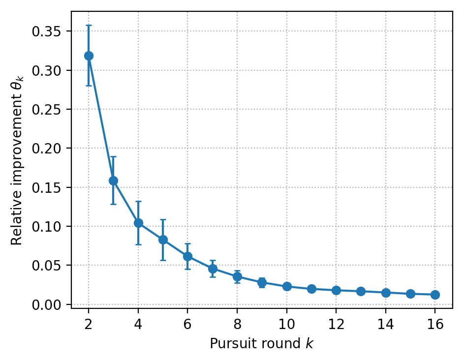
We define the relative improvement in alignment between rounds k−1k-1 and k∈⟦2,Kt⟧k\in\llbracket 2,K_{t}\rrbracket in the gradient pursuit procedure at iteration t∈⟦0,T−1⟧t\in\llbracket 0,T-1\rrbracket of BoostFW (Algorithm 2) as

θt,k≔align⁡(−∇f​(xt),dk)−align⁡(−∇f​(xt),dk−1)align⁡(−∇f​(xt),dk−1).\displaystyle\theta_{t,k}\coloneqq\frac{\operatorname{align}(-\nabla f(x_{t}),d_{k})-\operatorname{align}(-\nabla f(x_{t}),d_{k-1})}{\operatorname{align}(-\nabla f(x_{t}),d_{k-1})}.

For a fixed round kk, we plot in Figure 11 the mean of θt,k\theta_{t,k} across all iterations tt that performed a kk-th round, i.e.,

θk≔1|{t∈⟦0,T−1⟧∣k⩽Kt}|∑t=0T−1θt,k𝟙{k⩽Kt},\displaystyle\theta_{k}\coloneqq\frac{1}{|\{t\in\llbracket 0,T-1\rrbracket\mid k\leqslant K_{t}\}|}\sum_{t=0}^{T-1}\theta_{t,k}\mathds{1}_{\{k\leqslant K_{t}\}},

in the sparse signal recovery experiment (Section 4.1). The error bars represent ±1\pm 1 standard deviation. We see that on average the second round produces an improvement in alignment of ∼32%\sim 32\%, the third round produces an improvement of ∼16%\sim 16\%, etc. In particular, the plot could suggest that 77 rounds in each iteration are enough.

Refer to caption
Figure 11: Relative improvements in alignment during the gradient pursuit procedure of BoostFW.

In the traffic assignment experiment (Section 4.3), the FW oracle is particularly expensive so we decided to cap the maximum number of rounds KK. We plot in Figure 12 the relative improvements in alignment, and we chose to set K←5K\leftarrow 5.

Refer to caption
Figure 12: Traffic assignment (Section 4.3).

A.3 Computational experiments

Here we provide additional plots for each experiment of Section 4: comparisons in number of oracle calls and in duality gap. The duality gap is maxv∈𝒱⁡⟨∇f​(xt),xt−v⟩\max_{v\in\mathcal{V}}\langle\nabla f(x_{t}),x_{t}-v\rangle (Jaggi 2013) and we did not account for the CPU time taken to plot it. In number of oracle calls, the plots have a stair-like behavior as multiple calls can be made within an iteration. We see that BoostFW performs more oracle calls than the other methods in general however it converges faster both per iteration and in CPU time. Note that in the traffic assignment experiment (Figure 15), BoostFW also converges faster per oracle call. In the sparse logistic regression experiment (Figure 14), the line search-free strategies converge faster in CPU time and the line search strategies converge faster per iteration, but in the collaborative filtering experiment (Figure 16), BoostFW-ls and BoostFW-L respectively converge faster than expected.

Refer to caption
Refer to caption
Figure 13: Sparse signal recovery (Section 4.1).
Refer to caption
Refer to caption
Figure 14: Sparse logistic regression on the Gisette dataset (Section 4.2).
Refer to caption
Refer to caption
Figure 15: Traffic assignment (Section 4.3).
Refer to caption
Refer to caption
Figure 16: Collaborative filtering on the MovieLens 100k dataset (Section 4.4).
Refer to caption
Refer to caption
Figure 17: Video co-localization on the YouTube-Objects dataset (Section 4.5).

Appendix B Boosting DICG

We present an application of the boosting procedure to another Frank-Wolfe-style algorithm. Although the Away-Step and Pairwise Frank-Wolfe algorithms (Lacoste-Julien and Jaggi 2015) are more similar in essence to the vanilla Frank-Wolfe algorithm, we chose to apply our approach to the Decomposition-Invariant Pairwise Conditional Gradient (DICG) (Garber and Meshi 2016) because it does not need to maintain the decomposition of the iterates, which is a very favorable property in practice.

We recall DICG in Algorithm 3 and present our proposition for BoostDICG in Algorithm 4. Notice that since DICG moves in the pairwise direction vtFW−vtawayv_{t}^{\text{FW}}-v_{t}^{\text{away}}, in BoostDICG we chase the direction of −∇f​(xt)-\nabla f(x_{t}) from vtawayv_{t}^{\text{away}} (and not from xtx_{t}). Proposition B.1 shows that the iterates of BoostDICG are feasible. Similarly to DICG, BoostDICG is applicable only to polytopes of the form 𝒫={x∈ℝn∣Ax=b,x⩾0}\mathcal{P}=\{x\in\mathbb{R}^{n}\mid Ax=b,x\geqslant 0\} with set of vertices 𝒱⊆{0,1}n\mathcal{V}\subseteq\{0,1\}^{n}, and it does not need to maintain the decomposition of the iterates. See also Bashiri and Zhang 2017 for a follow-up work extending DICG to arbitrary polytopes.

Algorithm 3 Decomposition-Invariant Pairwise Conditional Gradient (DICG)

Input: Start point x0∈𝒫x_{0}\in\mathcal{P}.
Output: Point xT∈𝒫x_{T}\in\mathcal{P}.

1:  x1←arg​minv∈𝒱⁡⟨∇f​(x0),v⟩x_{1}\leftarrow\argmin\limits_{v\in\mathcal{V}}\langle\nabla f(x_{0}),v\rangle
2:  for t=1t=1 to T−1T-1 do
3:   vtFW←arg​minv∈𝒱⁡⟨∇f​(xt),v⟩v_{t}^{\text{FW}}\leftarrow\argmin\limits_{v\in\mathcal{V}}\langle\nabla f(x_{t}),v\rangle⊳\triangleright FW oracle
4:   [∇~f(xt)]i←{[∇f​(xt)]iif ​[xt]i>0−∞if ​[xt]i=0 for i∈⟦1,n⟧\left[\tilde{\nabla}f(x_{t})\right]_{i}\leftarrow\begin{cases}[\nabla f(x_{t})]_{i}&\textbf{if }[x_{t}]_{i}>0\\ -\infty&\textbf{if }[x_{t}]_{i}=0\end{cases}\quad\textbf{ for }i\in\llbracket 1,n\rrbracket
5:   vtaway←arg​maxv∈𝒱⁡⟨∇~​f​(xt),v⟩v_{t}^{\text{away}}\leftarrow\argmax\limits_{v\in\mathcal{V}}\langle\tilde{\nabla}f(x_{t}),v\rangle⊳\triangleright FW oracle
6:   γ¯t←max⁡{γ∈[0,1]∣xt+γ⁡(vtFW−vtaway)⩾0}\bar{\gamma}_{t}\leftarrow\max\{\gamma\in\left[0,1\right]\mid x_{t}+\gamma(v_{t}^{\text{FW}}-v_{t}^{\text{away}})\geqslant 0\}
7:   γt←arg​minγ∈[0,γ¯t]⁡f​(xt+γ⁡(vtFW−vtaway))\gamma_{t}\leftarrow\argmin\limits_{\gamma\in\left[0,\bar{\gamma}_{t}\right]}f(x_{t}+\gamma(v_{t}^{\text{FW}}-v_{t}^{\text{away}}))
8:   xt+1←xt+γt​(vtFW−vtaway)x_{t+1}\leftarrow x_{t}+\gamma_{t}(v_{t}^{\text{FW}}-v_{t}^{\text{away}})
9:  end for
Algorithm 4 Boosted Decomposition-Invariant Pairwise Conditional Gradient (BoostDICG)

Input: Input point y∈𝒞y\in\mathcal{C}, maximum number of rounds K∈ℕ\{0}K\in\mathbb{N}\backslash\{0\}, alignment improvement tolerance δ∈]0,1[\delta\in\left]0,1\right[, step-size strategy γt∈[0,1]\gamma_{t}\in\left[0,1\right].
Output: Point xT∈𝒫x_{T}\in\mathcal{P}.

1:  x0←arg​minv∈𝒱⁡⟨∇f​(y),v⟩x_{0}\leftarrow\argmin\limits_{v\in\mathcal{V}}\langle\nabla f(y),v\rangle
2:  for t=0t=0 to T−1T-1 do
3:   [∇~​f​(xt)]i←{[∇f​(xt)]iif ​[xt]i>0−∞if ​[xt]i=0\left[\tilde{\nabla}f(x_{t})\right]_{i}\leftarrow\begin{cases}[\nabla f(x_{t})]_{i}&\textbf{if }[x_{t}]_{i}>0\\ -\infty&\textbf{if }[x_{t}]_{i}=0\end{cases}\quad for i∈⟦1,n⟧i\in\llbracket 1,n\rrbracket
4:   vtaway←arg​maxv∈𝒱⁡⟨∇~​f​(xt),v⟩v_{t}^{\text{away}}\leftarrow\argmax\limits_{v\in\mathcal{V}}\langle\tilde{\nabla}f(x_{t}),v\rangle⊳\triangleright FW oracle
5:   d0←0d_{0}\leftarrow 0
6:   Λt←0\Lambda_{t}\leftarrow 0
7:   for k=0k=0 to K−1K-1 do
8:    rk←−∇f​(xt)−dkr_{k}\leftarrow-\nabla f(x_{t})-d_{k}⊳\triangleright kk-th residual
9:    vk←arg​maxv∈𝒱⁡⟨rk,v⟩v_{k}\leftarrow\argmax\limits_{v\in\mathcal{V}}\langle r_{k},v\rangle⊳\triangleright FW oracle
10:    uk←arg​maxu∈{vk−vtaway,−dk/∥dk∥}⟨rk,u⟩u_{k}\leftarrow\argmax\limits_{u\in\{v_{k}-v_{t}^{\text{away}},-d_{k}/\|d_{k}\|\}}\langle r_{k},u\rangle
11:    λk←⟨rk,uk⟩‖uk‖2\lambda_{k}\leftarrow\displaystyle\frac{\langle r_{k},u_{k}\rangle}{\|u_{k}\|^{2}}
12:    dk+1′←dk+λk​ukd_{k+1}^{\prime}\leftarrow d_{k}+\lambda_{k}u_{k}
13:    if align⁡(−∇f​(xt),dk+1′)−align⁡(−∇f​(xt),dk)⩾δ\operatorname{align}(-\nabla f(x_{t}),d_{k+1}^{\prime})-\operatorname{align}(-\nabla f(x_{t}),d_{k})\geqslant\delta then
14:     dk+1←dk+1′d_{k+1}\leftarrow d_{k+1}^{\prime}
15:     Λt←{Λt+λkif ​uk=vk−vtawayΛt​(1−λk/‖dk‖)if uk=−dk/∥dk∥\Lambda_{t}\leftarrow\begin{cases}\Lambda_{t}+\lambda_{k}&\textbf{if }u_{k}=v_{k}-v_{t}^{\text{away}}\\ \Lambda_{t}(1-\lambda_{k}/\|d_{k}\|)&\textbf{if }u_{k}=-d_{k}/\|d_{k}\|\end{cases}
16:    else
17:     break⊳\triangleright exit kk-loop
18:    end if
19:   end for
20:   Kt←kK_{t}\leftarrow k
21:   gt←dKt/Λtg_{t}\leftarrow d_{K_{t}}/\Lambda_{t}⊳\triangleright normalization
22:   γ¯t←max⁡{γ∈[0,1]∣xt+γ​gt⩾0}\bar{\gamma}_{t}\leftarrow\max\{\gamma\in\left[0,1\right]\mid x_{t}+\gamma g_{t}\geqslant 0\}
23:   γt←arg​minγ∈[0,γ¯t]⁡f​(xt+γ​gt)\gamma_{t}\leftarrow\argmin\limits_{\gamma\in\left[0,\bar{\gamma}_{t}\right]}f(x_{t}+\gamma g_{t})
24:   xt+1←xt+γt​gtx_{t+1}\leftarrow x_{t}+\gamma_{t}g_{t}
25:  end for
Proposition B.1.

The iterates of BoostDICG (Algorithm 4) are feasible.

Proof.

We proceed by induction. By definition, x0∈arg​minv∈𝒱⁡⟨∇f​(y),v⟩⊆𝒫x_{0}\in\argmin_{v\in\mathcal{V}}\langle\nabla f(y),v\rangle\subseteq\mathcal{P}. Let t∈⟦0,T−1⟧t\in\llbracket 0,T-1\rrbracket and suppose that xt∈𝒫x_{t}\in\mathcal{P}. Then xt+1←xt+γt​gtx_{t+1}\leftarrow x_{t}+\gamma_{t}g_{t} where γt∈[0,γ¯t]\gamma_{t}\in\left[0,\bar{\gamma}_{t}\right] and γ¯t←max⁡{γ∈[0,1]∣xt+γ​gt⩾0}\bar{\gamma}_{t}\leftarrow\max\{\gamma\in\left[0,1\right]\mid x_{t}+\gamma g_{t}\geqslant 0\}. Similarly to the proof of Proposition 3.1(iv), we can show that gt+vtaway∈𝒫g_{t}+v_{t}^{\text{away}}\in\mathcal{P}. Thus, since xt+1=xt+γt​((gt+vtaway)−vtaway)x_{t+1}=x_{t}+\gamma_{t}((g_{t}+v_{t}^{\text{away}})-v_{t}^{\text{away}}) and A​xt=bAx_{t}=b, A⁡(gt+vtaway)=bA(g_{t}+v_{t}^{\text{away}})=b, and A​vtaway=bAv_{t}^{\text{away}}=b by feasibility, we have A​xt+1=bAx_{t+1}=b. Lastly, xt+γ¯t​gt⩾0x_{t}+\bar{\gamma}_{t}g_{t}\geqslant 0 so, since xt⩾0x_{t}\geqslant 0 and γt∈[0,γ¯t]\gamma_{t}\in\left[0,\bar{\gamma}_{t}\right], we have xt+γt​gt⩾0x_{t}+\gamma_{t}g_{t}\geqslant 0, i.e., xt+1⩾0x_{t+1}\geqslant 0. Therefore, xt+1∈𝒫x_{t+1}\in\mathcal{P}. ∎

Appendix C A result on the Away-Step Frank-Wolfe algorithm

We first recall the Away-Step Frank-Wolfe algorithm (AFW) (Wolfe 1970) in Algorithm 5 and its convergence rate over polytopes with line search in Theorem C.2 (Lacoste-Julien and Jaggi 2015). This analysis is based on the pyramidal width of the polytope and the geometric strong convexity of the objective function (Lemma C.1). We refer the reader to Lacoste-Julien and Jaggi 2015 for the definition of the pyramidal width.

Let 𝒱⊂𝒫\mathcal{V}\subset\mathcal{P} denote the set of vertices of the polytope 𝒫\mathcal{P}. In Algorithm 5, λt∈ℝ|𝒱|\lambda_{t}\in\mathbb{R}^{|\mathcal{V}|} denotes the distribution of coefficients of the convex decomposition of xtx_{t} over 𝒱\mathcal{V} and λt​(v)\lambda_{t}(v) is the coefficient of vertex v∈𝒱v\in\mathcal{V} (as determined by the algorithm). Note that when an away step is taken and γt=γmax\gamma_{t}=\gamma_{\max}, then λt+1​(vtaway)=0\lambda_{t+1}(v_{t}^{\text{away}})=0 where vtaway∈𝒮tv_{t}^{\text{away}}\in\mathcal{S}_{t}. Thus, these steps always decrease the size of the active set: |𝒮t+1|<|𝒮t||\mathcal{S}_{t+1}|<|\mathcal{S}_{t}|. They are often referred to as drop steps.

Algorithm 5 Away-Step Frank-Wolfe (AFW)

Input: Start vertex x0∈𝒱x_{0}\in\mathcal{V}, step-size strategy γt∈[0,1]\gamma_{t}\in\left[0,1\right].
Output: Point xT∈𝒫x_{T}\in\mathcal{P}.

1:  𝒮0←{x0}\mathcal{S}_{0}\leftarrow\{x_{0}\}⊳\triangleright active set
2:  λ0←{𝟙{v=x0} for v∈𝒱}\lambda_{0}\leftarrow\{\mathds{1}_{\{v=x_{0}\}}\textbf{ for }v\in\mathcal{V}\}⊳\triangleright distribution of coefficients
3:  for t=0t=0 to T−1T-1 do
4:   vtFW←arg​minv∈𝒱⁡⟨∇f​(xt),v⟩v_{t}^{\text{FW}}\leftarrow\argmin\limits_{v\in\mathcal{V}}\langle\nabla f(x_{t}),v\rangle⊳\triangleright FW oracle
5:   vtaway←arg​maxv∈𝒮t⁡⟨∇f​(xt),v⟩v_{t}^{\text{away}}\leftarrow\argmax\limits_{v\in\mathcal{S}_{t}}\langle\nabla f(x_{t}),v\rangle
6:   if ⟨∇f​(xt),xt−vtFW⟩⩾⟨∇f​(xt),vtaway−xt⟩\langle\nabla f(x_{t}),x_{t}-v_{t}^{\text{FW}}\rangle\geqslant\langle\nabla f(x_{t}),v_{t}^{\text{away}}-x_{t}\rangle then
7:    xt+1←xt+γt​(vtFW−xt)x_{t+1}\leftarrow x_{t}+\gamma_{t}(v_{t}^{\text{FW}}-x_{t})⊳\triangleright FW step
8:    𝒮t+1←𝒮t∪{vtFW}\mathcal{S}_{t+1}\leftarrow\mathcal{S}_{t}\cup\{v_{t}^{\text{FW}}\}
9:    λt+1(v)←(1−γt)λt(v)+γt𝟙{v=vtFW} for v∈𝒮t+1\lambda_{t+1}(v)\leftarrow(1-\gamma_{t})\lambda_{t}(v)+\gamma_{t}\mathds{1}_{\{v=v_{t}^{\text{FW}}\}}\textbf{ for }v\in\mathcal{S}_{t+1}
10:   else
11:    γmax←λt​(vtaway)/(1−λt​(vtaway))\gamma_{\max}\leftarrow\lambda_{t}(v_{t}^{\text{away}})/(1-\lambda_{t}(v_{t}^{\text{away}}))
12:    xt+1←xt+γt​(xt−vtaway)x_{t+1}\leftarrow x_{t}+\gamma_{t}(x_{t}-v_{t}^{\text{away}})⊳\triangleright away step
13:    𝒮t+1←𝒮t\mathcal{S}_{t+1}\leftarrow\mathcal{S}_{t}
14:    λt+1(v)←(1+γt)λt(v)−γt𝟙{v=vtaway} for v∈𝒮t+1\lambda_{t+1}(v)\leftarrow(1+\gamma_{t})\lambda_{t}(v)-\gamma_{t}\mathds{1}_{\{v=v_{t}^{\text{away}}\}}\textbf{ for }v\in\mathcal{S}_{t+1}
15:   end if
16:   𝒮t+1←{v∈𝒮t+1∣λt+1​(v)>0}\mathcal{S}_{t+1}\leftarrow\{v\in\mathcal{S}_{t+1}\mid\lambda_{t+1}(v)>0\}
17:  end for
Lemma C.1 ((Lacoste-Julien and Jaggi 2015, Equations (28) and (23))).

Let 𝒫⊂ℝn\mathcal{P}\subset\mathbb{R}^{n} be a polytope with pyramidal width W>0W>0 and f:ℝn→ℝf:\mathbb{R}^{n}\rightarrow\mathbb{R} be a SS-strongly convex function. Then the Away-Step Frank-Wolfe algorithm (AFW, Algorithm 5) ensures for all t∈⟦0,T−1⟧t\in\llbracket 0,T-1\rrbracket,

f⁡(xt)−min𝒫⁡f⩽⟨∇f​(xt),vtaway−vtFW⟩22​S​W2.\displaystyle f(x_{t})-\min_{\mathcal{P}}f\leqslant\frac{\langle\nabla f(x_{t}),v_{t}^{\text{away}}-v_{t}^{\text{FW}}\rangle^{2}}{2SW^{2}}.
Theorem C.2 ((AFW with line search, Lacoste-Julien and Jaggi 2015)).

Let 𝒫⊂ℝn\mathcal{P}\subset\mathbb{R}^{n} be a polytope and f:ℝn→ℝf:\mathbb{R}^{n}\rightarrow\mathbb{R} be a LL-smooth and SS-strongly convex function. Consider the Away-Step Frank-Wolfe algorithm (AFW, Algorithm 5) with the line search strategy

γt←{arg​minγ∈[0,1]⁡f​(xt+γt​(vtFW−xt))in the case of a FW step (Line 7)arg​minγ∈[0,γmax]⁡f​(xt+γt​(xt−vtaway))in the case of an away step (Line 12).\displaystyle\gamma_{t}\leftarrow\begin{cases}\argmin_{\gamma\in\left[0,1\right]}f(x_{t}+\gamma_{t}(v_{t}^{\text{FW}}-x_{t}))&\text{in the case of a FW step (Line~\ref{afw:fw})}\\ \argmin_{\gamma\in\left[0,\gamma_{\max}\right]}f(x_{t}+\gamma_{t}(x_{t}-v_{t}^{\text{away}}))&\text{in the case of an away step (Line~\ref{afw:away})}.\end{cases}

Then for all t∈⟦0,T⟧t\in\llbracket 0,T\rrbracket,

f⁡(xt)−min𝒫⁡f⩽(1−S4​L​(WD)2)t/2​(f⁡(x0)−min𝒫⁡f)\displaystyle f(x_{t})-\min_{\mathcal{P}}f\leqslant\left(1-\frac{S}{4L}\left(\frac{W}{D}\right)^{2}\right)^{t/2}\left(f(x_{0})-\min_{\mathcal{P}}f\right)

where DD and WW are the diameter and the pyramidal width of 𝒫\mathcal{P} respectively.

We now show in Theorem C.3 that AFW can also achieve the convergence rate of Theorem C.2 without line search, by using the short step strategy. We were later informed that this result was already derived by Pedregosa et al. 2020 in a more general setting.

Theorem C.3 ((AFW with short steps)).

Let 𝒫⊂ℝn\mathcal{P}\subset\mathbb{R}^{n} be a polytope and f:ℝn→ℝf:\mathbb{R}^{n}\rightarrow\mathbb{R} be a LL-smooth and SS-strongly convex function. Consider the Away-Step Frank-Wolfe algorithm (AFW, Algorithm 5) with the step-size strategy

γt←{min⁡{⟨∇f​(xt),xt−vtFW⟩L​‖xt−vtFW‖22,1}in the case of a FW step (Line 7)min⁡{⟨∇f​(xt),vtaway−xt⟩L​‖vtaway−xt‖22,γmax}in the case of an away step (Line 12).\displaystyle\gamma_{t}\leftarrow\begin{cases}\displaystyle\min\left\{\frac{\langle\nabla f(x_{t}),x_{t}-v_{t}^{\text{FW}}\rangle}{L\|x_{t}-v_{t}^{\text{FW}}\|_{2}^{2}},1\right\}&\text{in the case of a FW step (Line~\ref{afw:fw})}\\ \displaystyle\min\left\{\frac{\langle\nabla f(x_{t}),v_{t}^{\text{away}}-x_{t}\rangle}{L\|v_{t}^{\text{away}}-x_{t}\|_{2}^{2}},\gamma_{\max}\right\}&\text{in the case of an away step (Line~\ref{afw:away})}.\end{cases} (7)

Then for all t∈⟦0,T⟧t\in\llbracket 0,T\rrbracket,

f⁡(xt)−min𝒫⁡f⩽(1−S4​L​(WD)2)t/2​(f⁡(x0)−min𝒫⁡f)\displaystyle f(x_{t})-\min_{\mathcal{P}}f\leqslant\left(1-\frac{S}{4L}\left(\frac{W}{D}\right)^{2}\right)^{t/2}\left(f(x_{0})-\min_{\mathcal{P}}f\right)

where DD and WW are the diameter and the pyramidal width of 𝒫\mathcal{P} respectively.

Proof.

Let t∈⟦0,T−1⟧t\in\llbracket 0,T-1\rrbracket and denote εt≔f⁡(xt)−min𝒫⁡f\varepsilon_{t}\coloneqq f(x_{t})-\min_{\mathcal{P}}f. By geometric strong convexity (Lemma C.1),

εt⩽⟨∇f​(xt),vtaway−vtFW⟩22​S​W2.\displaystyle\varepsilon_{t}\leqslant\frac{\langle\nabla f(x_{t}),v_{t}^{\text{away}}-v_{t}^{\text{FW}}\rangle^{2}}{2SW^{2}}. (8)

Furthermore, since

⟨∇f​(xt),vtaway−vtFW⟩=⟨∇f​(xt),vtaway−xt⟩+⟨∇f​(xt),xt−vtFW⟩⩾0\displaystyle\langle\nabla f(x_{t}),v_{t}^{\text{away}}-v_{t}^{\text{FW}}\rangle=\langle\nabla f(x_{t}),v_{t}^{\text{away}}-x_{t}\rangle+\langle\nabla f(x_{t}),x_{t}-v_{t}^{\text{FW}}\rangle\geqslant 0

we have

max⁡{⟨∇f​(xt),vtaway−xt⟩,⟨∇f​(xt),xt−vtFW⟩}⩾⟨∇f​(xt),vtaway−vtFW⟩2⩾0.\displaystyle\max\{\langle\nabla f(x_{t}),v_{t}^{\text{away}}-x_{t}\rangle,\langle\nabla f(x_{t}),x_{t}-v_{t}^{\text{FW}}\rangle\}\geqslant\frac{\langle\nabla f(x_{t}),v_{t}^{\text{away}}-v_{t}^{\text{FW}}\rangle}{2}\geqslant 0. (9)

Note that AFW performs a step corresponding to max⁡{⟨∇f​(xt),vtaway−xt⟩,⟨∇f​(xt),xt−vtFW⟩}\max\{\langle\nabla f(x_{t}),v_{t}^{\text{away}}-x_{t}\rangle,\langle\nabla f(x_{t}),x_{t}-v_{t}^{\text{FW}}\rangle\} (Lines 6 and 10).

FW step. In the case where the algorithm performs a FW step, we have γt←min⁡{⟨∇f​(xt),xt−vtFW⟩/(L​‖xt−vtFW‖22),1}\gamma_{t}\leftarrow\min\{\langle\nabla f(x_{t}),x_{t}-v_{t}^{\text{FW}}\rangle/(L\|x_{t}-v_{t}^{\text{FW}}\|_{2}^{2}),1\}, xt+1←xt+γt​(vtFW−xt)x_{t+1}\leftarrow x_{t}+\gamma_{t}(v_{t}^{\text{FW}}-x_{t}), and by Line 6 and (9),

⟨∇f​(xt),xt−vtFW⟩⩾⟨∇f​(xt),vtaway−vtFW⟩2⩾0.\displaystyle\langle\nabla f(x_{t}),x_{t}-v_{t}^{\text{FW}}\rangle\geqslant\frac{\langle\nabla f(x_{t}),v_{t}^{\text{away}}-v_{t}^{\text{FW}}\rangle}{2}\geqslant 0. (10)

By smoothness of ff,

εt+1⩽εt+γt​⟨∇f​(xt),vtFW−xt⟩+L2​γt2​‖vtFW−xt‖22.\displaystyle\varepsilon_{t+1}\leqslant\varepsilon_{t}+\gamma_{t}\langle\nabla f(x_{t}),v_{t}^{\text{FW}}-x_{t}\rangle+\frac{L}{2}\gamma_{t}^{2}\|v_{t}^{\text{FW}}-x_{t}\|_{2}^{2}. (11)

Consider the choice of step-size (7) and suppose γt<1\gamma_{t}<1. Then, with (10) and (8),

εt+1\displaystyle\varepsilon_{t+1} ⩽εt−⟨∇f​(xt),xt−vtFW⟩22​L​‖xt−vtFW‖22\displaystyle\leqslant\varepsilon_{t}-\frac{\langle\nabla f(x_{t}),x_{t}-v_{t}^{\text{FW}}\rangle^{2}}{2L\|x_{t}-v_{t}^{\text{FW}}\|_{2}^{2}}
⩽εt−⟨∇f​(xt),vtaway−vtFW⟩28​L​D2\displaystyle\leqslant\varepsilon_{t}-\frac{\langle\nabla f(x_{t}),v_{t}^{\text{away}}-v_{t}^{\text{FW}}\rangle^{2}}{8LD^{2}}
⩽(1−S4​L​(WD)2)​εt.\displaystyle\leqslant\left(1-\frac{S}{4L}\left(\frac{W}{D}\right)^{2}\right)\varepsilon_{t}.

If γt=1\gamma_{t}=1 then ⟨∇f​(xt),xt−vtFW⟩⩾L​‖xt−vtFW‖22\langle\nabla f(x_{t}),x_{t}-v_{t}^{\text{FW}}\rangle\geqslant L\|x_{t}-v_{t}^{\text{FW}}\|_{2}^{2}. By (11), the optimality of vtFWv_{t}^{\text{FW}} (Line 4), and the convexity of ff,

εt+1\displaystyle\varepsilon_{t+1} ⩽εt+⟨∇f​(xt),vtFW−xt⟩+L2​‖vtFW−xt‖22\displaystyle\leqslant\varepsilon_{t}+\langle\nabla f(x_{t}),v_{t}^{\text{FW}}-x_{t}\rangle+\frac{L}{2}\|v_{t}^{\text{FW}}-x_{t}\|_{2}^{2}
⩽εt+⟨∇f​(xt),vtFW−xt⟩2\displaystyle\leqslant\varepsilon_{t}+\frac{\langle\nabla f(x_{t}),v_{t}^{\text{FW}}-x_{t}\rangle}{2}
⩽εt+⟨∇f​(xt),x∗−xt⟩2\displaystyle\leqslant\varepsilon_{t}+\frac{\langle\nabla f(x_{t}),x^{*}-x_{t}\rangle}{2}
⩽εt2.\displaystyle\leqslant\frac{\varepsilon_{t}}{2}.

Therefore, the progress obtain by a FW step is

εt+1\displaystyle\varepsilon_{t+1} ⩽(1−min⁡{12,S4​L​(WD)2})​εt\displaystyle\leqslant\left(1-\min\left\{\frac{1}{2},\frac{S}{4L}\left(\frac{W}{D}\right)^{2}\right\}\right)\varepsilon_{t}
=(1−S4​L​(WD)2)​εt\displaystyle=\left(1-\frac{S}{4L}\left(\frac{W}{D}\right)^{2}\right)\varepsilon_{t} (12)

since S⩽LS\leqslant L and W⩽DW\leqslant D.

Away step. In the case where the algorithm performs an away step, we have γt←min⁡{⟨∇f​(xt),vtaway−xt⟩/(L​‖vtaway−xt‖22),γmax}\gamma_{t}\leftarrow\min\{\langle\nabla f(x_{t}),v_{t}^{\text{away}}-x_{t}\rangle/(L\|v_{t}^{\text{away}}-x_{t}\|_{2}^{2}),\gamma_{\max}\}, xt+1←xt+γt​(xt−vtaway)x_{t+1}\leftarrow x_{t}+\gamma_{t}(x_{t}-v_{t}^{\text{away}}), and by Line 6 and (9),

⟨∇f​(xt),vtaway−xt⟩⩾⟨∇f​(xt),vtaway−vtFW⟩2⩾0.\displaystyle\langle\nabla f(x_{t}),v_{t}^{\text{away}}-x_{t}\rangle\geqslant\frac{\langle\nabla f(x_{t}),v_{t}^{\text{away}}-v_{t}^{\text{FW}}\rangle}{2}\geqslant 0. (13)

By smoothness of ff,

εt+1⩽εt+γt​⟨∇f​(xt),xt−vtaway⟩+L2​γt2​‖xt−vtaway‖22\displaystyle\varepsilon_{t+1}\leqslant\varepsilon_{t}+\gamma_{t}\langle\nabla f(x_{t}),x_{t}-v_{t}^{\text{away}}\rangle+\frac{L}{2}\gamma_{t}^{2}\|x_{t}-v_{t}^{\text{away}}\|_{2}^{2} (14)

Consider the choice of step-size (7) and suppose γt<γmax\gamma_{t}<\gamma_{\max}. Then, with (13) and (8),

εt+1\displaystyle\varepsilon_{t+1} ⩽εt−⟨∇f​(xt),vtaway−xt⟩22​L​‖vtaway−xt‖22\displaystyle\leqslant\varepsilon_{t}-\frac{\langle\nabla f(x_{t}),v_{t}^{\text{away}}-x_{t}\rangle^{2}}{2L\|v_{t}^{\text{away}}-x_{t}\|_{2}^{2}}
⩽εt−⟨∇f​(xt),vtaway−vtFW⟩28​L​D2\displaystyle\leqslant\varepsilon_{t}-\frac{\langle\nabla f(x_{t}),v_{t}^{\text{away}}-v_{t}^{\text{FW}}\rangle^{2}}{8LD^{2}}
⩽(1−S4​L​(WD)2)​εt.\displaystyle\leqslant\left(1-\frac{S}{4L}\left(\frac{W}{D}\right)^{2}\right)\varepsilon_{t}. (15)

If γt=γmax\gamma_{t}=\gamma_{\max} then γmax⩽γt∗≔⟨∇f​(xt),vtaway−xt⟩/(L​‖vtaway−xt‖22)\gamma_{\max}\leqslant\gamma_{t}^{*}\coloneqq\langle\nabla f(x_{t}),v_{t}^{\text{away}}-x_{t}\rangle/(L\|v_{t}^{\text{away}}-x_{t}\|_{2}^{2}). Let φt:γ∈[0,γt∗]↦γ⁡⟨∇f​(xt),xt−vtaway⟩+L​γ2​‖xt−vtaway‖22/2\varphi_{t}:\gamma\in\left[0,\gamma_{t}^{*}\right]\mapsto\gamma\langle\nabla f(x_{t}),x_{t}-v_{t}^{\text{away}}\rangle+L\gamma^{2}\|x_{t}-v_{t}^{\text{away}}\|_{2}^{2}/2. By (14),

εt+1⩽εt+φt​(γmax).\displaystyle\varepsilon_{t+1}\leqslant\varepsilon_{t}+\varphi_{t}(\gamma_{\max}).

The quadratic function φt\varphi_{t} attains its unique global minimum at γ=γt∗\gamma=\gamma_{t}^{*} and satisfies φt(γt∗)=−⟨∇f(xt),xt−vtaway⟩2/(2L∥xt−vtaway∥22)⩽0\varphi_{t}(\gamma_{t}^{*})=-\langle\nabla f(x_{t}),x_{t}-v_{t}^{\text{away}}\rangle^{2}/(2L\|x_{t}-v_{t}^{\text{away}}\|_{2}^{2})\leqslant 0 and φt​(0)=0\varphi_{t}(0)=0. Since γmax∈[0,γt∗]\gamma_{\max}\in\left[0,\gamma_{t}^{*}\right], we have φt​(γmax)⩽0\varphi_{t}(\gamma_{\max})\leqslant 0 so

εt+1⩽εt\displaystyle\varepsilon_{t+1}\leqslant\varepsilon_{t} (16)

which shows that the progress is always nonnegative.

Wrapping up. Since the steps with progress (16) always decrease the number of vertices in the active set 𝒮t\mathcal{S}_{t}, there are at most ⌊t/2⌋\lfloor t/2\rfloor after tt iterations. By (12) and (15), we conclude that

εt⩽(1−S4​L​(WD)2)⌈t/2⌉​ε0⩽(1−S4​L​(WD)2)t/2​ε0.\displaystyle\varepsilon_{t}\leqslant\left(1-\frac{S}{4L}\left(\frac{W}{D}\right)^{2}\right)^{\lceil t/2\rceil}\varepsilon_{0}\leqslant\left(1-\frac{S}{4L}\left(\frac{W}{D}\right)^{2}\right)^{t/2}\varepsilon_{0}.

∎

Appendix D Proofs

D.1 Preliminaries

Fact D.1 ((Fact 2.1)).

Let f:ℋ→ℝf:\mathcal{H}\rightarrow\mathbb{R} be SS-strongly convex. Then ff is SS-gradient dominated.

Proof.

The function ff is strongly convex hence it has a unique minimizer, which we denote by x∗∈ℋx^{*}\in\mathcal{H}. Let x∈ℋx\in\mathcal{H}. By strong convexity, for all y∈ℋy\in\mathcal{H} we have

f⁡(y)⩾f⁡(x)+⟨∇f​(x),y−x⟩+S2​‖y−x‖2.\displaystyle f(y)\geqslant f(x)+\langle\nabla f(x),y-x\rangle+\frac{S}{2}\|y-x\|^{2}.

Now we minimize both sides with respect to y∈ℋy\in\mathcal{H}. The left-hand side is minimized for y=x∗y=x^{*} and the right-hand side is minimized for y=x−∇f​(x)/Sy=x-\nabla f(x)/S. Thus,

f⁡(x∗)⩾f⁡(x)−‖∇f​(x)‖22​S\displaystyle f(x^{*})\geqslant f(x)-\frac{\|\nabla f(x)\|^{2}}{2S}

i.e.,

f⁡(x)−minℋ⁡f⩽‖∇f​(x)‖22​S.\displaystyle f(x)-\min_{\mathcal{H}}f\leqslant\frac{\|\nabla f(x)\|^{2}}{2S}.

∎

D.2 Boosting via gradient pursuit

Proposition D.2 ((Proposition 3.1)).

Let t∈⟦0,T−1⟧t\in\llbracket 0,T-1\rrbracket and suppose that xt∈𝒞x_{t}\in\mathcal{C}. Then:

  1. (i)

    d1d_{1} is defined and Kt⩾1K_{t}\geqslant 1,

  2. (ii)

    λ0,…,λKt−1⩾0\lambda_{0},\ldots,\lambda_{K_{t}-1}\geqslant 0,

  3. (iii)

    dk∈cone⁡(𝒱−xt)d_{k}\in\operatorname{cone}(\mathcal{V}-x_{t}) for all k∈⟦0,Kt⟧k\in\llbracket 0,K_{t}\rrbracket,

  4. (iv)

    xt+gt∈𝒞x_{t}+g_{t}\in\mathcal{C} and xt+1∈𝒞x_{t+1}\in\mathcal{C},

  5. (v)

    align⁡(−∇f​(xt),gt)⩾align⁡(−∇f​(xt),vt−xt)+(Kt−1)​δ\operatorname{align}(-\nabla f(x_{t}),g_{t})\geqslant\operatorname{align}(-\nabla f(x_{t}),v_{t}-x_{t})+(K_{t}-1)\delta where vt∈arg​minv∈𝒱⁡⟨∇f​(xt),v⟩v_{t}\in\argmin_{v\in\mathcal{V}}\langle\nabla f(x_{t}),v\rangle and align⁡(−∇f​(xt),vt−xt)⩾0\operatorname{align}(-\nabla f(x_{t}),v_{t}-x_{t})\geqslant 0.

Since x0∈𝒞x_{0}\in\mathcal{C}, these properties are satisfied for all t∈⟦0,T−1⟧t\in\llbracket 0,T-1\rrbracket by induction.

Proof.

We analyze BoostFW (Algorithm 2).

  1. (i)

    We have d0=0d_{0}=0 so r0=−∇f​(xt)r_{0}=-\nabla f(x_{t}) and align⁡(r0,d0)=−1\operatorname{align}(r_{0},d_{0})=-1 by definition (3). Furthermore, since v0∈arg​maxv∈𝒱⁡⟨r0,v⟩v_{0}\in\argmax_{v\in\mathcal{V}}\langle r_{0},v\rangle and xt∈𝒞x_{t}\in\mathcal{C}, we have

    ⟨r0,v0−xt⟩=⟨r0,v0⟩−⟨r0,xt⟩⩾0\displaystyle\langle r_{0},v_{0}-x_{t}\rangle=\langle r_{0},v_{0}\rangle-\langle r_{0},x_{t}\rangle\geqslant 0

    so u0=v0−xtu_{0}=v_{0}-x_{t} by Line 9 since d0=0d_{0}=0. Thus, λ0⩾0\lambda_{0}\geqslant 0 (Line 10) and d1′=λ0​(v0−xt)d_{1}^{\prime}=\lambda_{0}(v_{0}-x_{t}) (Line 11) so

    align⁡(−∇f​(xt),d1′)\displaystyle\operatorname{align}(-\nabla f(x_{t}),d_{1}^{\prime}) =⟨−∇f​(xt),d1′⟩‖∇f​(xt)‖​‖d1′‖\displaystyle=\frac{\langle-\nabla f(x_{t}),d_{1}^{\prime}\rangle}{\|\nabla f(x_{t})\|\|d_{1}^{\prime}\|}
    =⟨r0,v0−xt⟩‖r0‖​‖v0−xt‖\displaystyle=\frac{\langle r_{0},v_{0}-x_{t}\rangle}{\|r_{0}\|\|v_{0}-x_{t}\|}
    ⩾0\displaystyle\geqslant 0
    ⩾−1+δ\displaystyle\geqslant-1+\delta
    =align⁡(−∇f​(xt),d0)+δ.\displaystyle=\operatorname{align}(-\nabla f(x_{t}),d_{0})+\delta.

    Therefore, by Line 12 the gradient pursuit procedure continues.

  2. (ii)

    Let k∈⟦0,Kt−1⟧k\in\llbracket 0,K_{t}-1\rrbracket. Since vk∈arg​maxv∈𝒱⁡⟨rk,v⟩v_{k}\in\argmax_{v\in\mathcal{V}}\langle r_{k},v\rangle (Line 8) and xt∈conv⁡(𝒱)=𝒞x_{t}\in\operatorname{conv}(\mathcal{V})=\mathcal{C},

    ⟨rk,vk−xt⟩=maxv∈𝒱⁡⟨rk,v⟩−⟨rk,xt⟩⩾0.\displaystyle\langle r_{k},v_{k}-x_{t}\rangle=\max_{v\in\mathcal{V}}\langle r_{k},v\rangle-\langle r_{k},x_{t}\rangle\geqslant 0.

    Thus, by Lines 9-10 we have

    λk=⟨rk,uk⟩‖uk‖2⩾0.\displaystyle\lambda_{k}=\frac{\langle r_{k},u_{k}\rangle}{\|u_{k}\|^{2}}\geqslant 0.

    Furthermore, note that −rk-r_{k} is the gradient of the objective function in subproblem (2) and ⟨rk,uk⟩\langle r_{k},u_{k}\rangle is a scaled upper bound on its primal gap (Locatello et al. 2017). Thus, if λk=0\lambda_{k}=0 then the gradient pursuit procedure has already converged.

  3. (iii)

    We show by induction that dk∈cone⁡(𝒱−xt)d_{k}\in\operatorname{cone}(\mathcal{V}-x_{t}) for all k∈⟦0,Kt⟧k\in\llbracket 0,K_{t}\rrbracket. We have d0=0∈cone⁡(𝒱−xt)d_{0}=0\in\operatorname{cone}(\mathcal{V}-x_{t}) so the base case is satisfied. Suppose that dk∈cone⁡(𝒱−xt)d_{k}\in\operatorname{cone}(\mathcal{V}-x_{t}) for some k∈⟦0,Kt−1⟧k\in\llbracket 0,K_{t}-1\rrbracket. If uk=vk−xtu_{k}=v_{k}-x_{t} then uk∈𝒱−xtu_{k}\in\mathcal{V}-x_{t} and since λk⩾0\lambda_{k}\geqslant 0 by (ii), we have dk+1=dk+λk​(vk−xt)∈cone⁡(𝒱−xt)d_{k+1}=d_{k}+\lambda_{k}(v_{k}-x_{t})\in\operatorname{cone}(\mathcal{V}-x_{t}). Else, uk=−dk/∥dk∥u_{k}=-d_{k}/\|d_{k}\| so dk+1=(1−λk/‖dk‖)​dkd_{k+1}=(1-\lambda_{k}/\|d_{k}\|)d_{k} and it remains to show that 1−λk/‖dk‖⩾01-\lambda_{k}/\|d_{k}\|\geqslant 0. We will show that 1−λk/‖dk‖⩾1/21-\lambda_{k}/\|d_{k}\|\geqslant 1/2. We have

    1−λk‖dk‖⩾12\displaystyle 1-\frac{\lambda_{k}}{\|d_{k}\|}\geqslant\frac{1}{2} ⇔12⩾λk‖dk‖=⟨rk,−dk/∥dk∥⟩‖dk‖\displaystyle\Leftrightarrow\frac{1}{2}\geqslant\frac{\lambda_{k}}{\|d_{k}\|}=\frac{\langle r_{k},-d_{k}/\|d_{k}\|\rangle}{\|d_{k}\|}
    ⇔‖dk‖22⩾⟨rk,−dk⟩.\displaystyle\Leftrightarrow\frac{\|d_{k}\|^{2}}{2}\geqslant\langle r_{k},-d_{k}\rangle. (17)

    so it suffices to show that ‖dk‖2/2⩾⟨rk,−dk⟩\|d_{k}\|^{2}/2\geqslant\langle r_{k},-d_{k}\rangle. Now, the procedure satisfies for all k′∈⟦0,Kt−1⟧k^{\prime}\in\llbracket 0,K_{t}-1\rrbracket,

    ‖rk′+1‖2\displaystyle\|r_{k^{\prime}+1}\|^{2} =‖rk′−λk′​uk′‖2\displaystyle=\|r_{k^{\prime}}-\lambda_{k^{\prime}}u_{k^{\prime}}\|^{2}
    =‖rk′‖2−2​λk′​⟨rk′,uk′⟩+λk′2​‖uk′‖2\displaystyle=\|r_{k^{\prime}}\|^{2}-2\lambda_{k^{\prime}}\langle r_{k^{\prime}},u_{k^{\prime}}\rangle+\lambda_{k^{\prime}}^{2}\|u_{k^{\prime}}\|^{2}
    =‖rk′‖2−⟨rk′,uk′⟩2‖uk′‖2\displaystyle=\|r_{k^{\prime}}\|^{2}-\frac{\langle r_{k^{\prime}},u_{k^{\prime}}\rangle^{2}}{\|u_{k^{\prime}}\|^{2}}
    ⩽‖rk′‖2\displaystyle\leqslant\|r_{k^{\prime}}\|^{2}

    where we used λk′=⟨rk′,uk′⟩/‖uk′‖2\lambda_{k^{\prime}}=\langle r_{k^{\prime}},u_{k^{\prime}}\rangle/\|u_{k^{\prime}}\|^{2}. Thus ‖rk‖2⩽‖r0‖2\|r_{k}\|^{2}\leqslant\|r_{0}\|^{2}, i.e., since d0=0d_{0}=0, ‖∇f​(xt)+dk‖2⩽‖∇f​(xt)‖2\|\nabla f(x_{t})+d_{k}\|^{2}\leqslant\|\nabla f(x_{t})\|^{2} so

    ‖∇f​(xt)‖2⩾‖∇f​(xt)+dk‖2=‖∇f​(xt)‖2+2​⟨∇f​(xt),dk⟩+‖dk‖2\displaystyle\|\nabla f(x_{t})\|^{2}\geqslant\|\nabla f(x_{t})+d_{k}\|^{2}=\|\nabla f(x_{t})\|^{2}+2\langle\nabla f(x_{t}),d_{k}\rangle+\|d_{k}\|^{2}

    hence

    ⟨∇f​(xt),dk⟩⩽−‖dk‖22.\displaystyle\langle\nabla f(x_{t}),d_{k}\rangle\leqslant-\frac{\|d_{k}\|^{2}}{2}.

    Thus,

    ⟨rk,−dk⟩\displaystyle\langle r_{k},-d_{k}\rangle =⟨∇f​(xt)+dk,dk⟩\displaystyle=\langle\nabla f(x_{t})+d_{k},d_{k}\rangle
    =⟨∇f​(xt),dk⟩+‖dk‖2\displaystyle=\langle\nabla f(x_{t}),d_{k}\rangle+\|d_{k}\|^{2}
    ⩽‖dk‖22.\displaystyle\leqslant\frac{\|d_{k}\|^{2}}{2}.

    Therefore, with (17) we can conclude that dk+1∈cone⁡(𝒱−xt)d_{k+1}\in\operatorname{cone}(\mathcal{V}-x_{t}).

  4. (iv)

    By (iii), dKt∈cone⁡(𝒱−xt)d_{K_{t}}\in\operatorname{cone}(\mathcal{V}-x_{t}) so since gt=dKt/Λtg_{t}=d_{K_{t}}/\Lambda_{t}, to show that xt+gt∈𝒞x_{t}+g_{t}\in\mathcal{C} it suffices to show that the sum of coefficients in the conical decomposition of dKtd_{K_{t}} is equal to Λt\Lambda_{t}, and then it follows that gt∈conv⁡(𝒱−xt)=conv⁡(𝒱)−xt=𝒞−xtg_{t}\in\operatorname{conv}(\mathcal{V}-x_{t})=\operatorname{conv}(\mathcal{V})-x_{t}=\mathcal{C}-x_{t}. By Line 14, this is true and is verified by a simple induction on kk: the base case is satisfied and if uk=vk−xtu_{k}=v_{k}-x_{t} then dk+1=dk+λk​(vk−xt)d_{k+1}=d_{k}+\lambda_{k}(v_{k}-x_{t}) and Line 14 shows that Λt←Λt+λk\Lambda_{t}\leftarrow\Lambda_{t}+\lambda_{k} is updated accordingly, else uk=−dk/∥dk∥u_{k}=-d_{k}/\|d_{k}\| so dk+1=(1−λk/‖dk‖)​dkd_{k+1}=(1-\lambda_{k}/\|d_{k}\|)d_{k} and Line 14 shows that Λt←Λt​(1−λk/‖dk‖)\Lambda_{t}\leftarrow\Lambda_{t}(1-\lambda_{k}/\|d_{k}\|) is again updated accordingly. Thus, xt+gt∈𝒞x_{t}+g_{t}\in\mathcal{C}. Then,

    xt+1\displaystyle x_{t+1} =xt+γt​gt\displaystyle=x_{t}+\gamma_{t}g_{t}
    =xt+γt​((xt+gt)−xt)\displaystyle=x_{t}+\gamma_{t}((x_{t}+g_{t})-x_{t})
    =(1−γt)​xt+γt​(xt+gt)⏟∈𝒞.\displaystyle=(1-\gamma_{t})x_{t}+\gamma_{t}\underbrace{(x_{t}+g_{t})}_{\in\mathcal{C}}.

    Since γt∈[0,1]\gamma_{t}\in\left[0,1\right], we conclude that xt+1∈𝒞x_{t+1}\in\mathcal{C} by convex combination.

  5. (v)

    Since d0=0d_{0}=0, we have r0=−∇f​(xt)r_{0}=-\nabla f(x_{t}) so by Line 8, v0∈arg​minv∈𝒱⁡⟨∇f​(xt),v⟩v_{0}\in\argmin_{v\in\mathcal{V}}\langle\nabla f(x_{t}),v\rangle, and we have d1=vt−xtd_{1}=v_{t}-x_{t}. Let vt≔v0v_{t}\coloneqq v_{0}. Since gt=dKt/Λtg_{t}=d_{K_{t}}/\Lambda_{t} where Kt⩾1K_{t}\geqslant 1 by (i), by Line 12 we obtain

    align⁡(−∇f​(xt),gt)\displaystyle\operatorname{align}(-\nabla f(x_{t}),g_{t}) =align⁡(−∇f​(xt),dKt)\displaystyle=\operatorname{align}(-\nabla f(x_{t}),d_{K_{t}})
    ⩾align⁡(−∇f​(xt),vt−xt)+(Kt−1)​δ.\displaystyle\geqslant\operatorname{align}(-\nabla f(x_{t}),v_{t}-x_{t})+(K_{t}-1)\delta.

    Lastly,

    align⁡(−∇f​(xt),vt−xt)\displaystyle\operatorname{align}(-\nabla f(x_{t}),v_{t}-x_{t}) =⟨∇f​(xt),xt−vt⟩‖∇f​(xt)‖​‖xt−vt‖\displaystyle=\frac{\langle\nabla f(x_{t}),x_{t}-v_{t}\rangle}{\|\nabla f(x_{t})\|\|x_{t}-v_{t}\|}
    ⩾0\displaystyle\geqslant 0

    because ⟨∇f​(xt),xt−vt⟩⩾0\langle\nabla f(x_{t}),x_{t}-v_{t}\rangle\geqslant 0 since xt∈𝒞x_{t}\in\mathcal{C}.

∎

D.3 Convergence analysis

Theorem D.3 ((Theorem 3.2)).

Let f:ℋ→ℝf:\mathcal{H}\rightarrow\mathbb{R} be LL-smooth, convex, and μ\mu-gradient dominated, and set γt←min⁡{ηt​‖∇f​(xt)‖/(L​‖gt‖),1}\gamma_{t}\leftarrow\min\{\eta_{t}\|\nabla f(x_{t})\|/(L\|g_{t}\|),1\} or γt←arg​minγ∈[0,1]⁡f​(xt+γ​gt)\gamma_{t}\leftarrow\argmin_{\gamma\in\left[0,1\right]}f(x_{t}+\gamma g_{t}). Then for all t∈⟦0,T⟧t\in\llbracket 0,T\rrbracket,

f(xt)−min𝒞f⩽L​D22∏s=0t−1(1−ηs2μL)𝟙{γs<1}(1−‖gs‖2​‖vs−xs‖)𝟙{γs=1}\displaystyle f(x_{t})-\min_{\mathcal{C}}f\leqslant\frac{LD^{2}}{2}\prod_{s=0}^{t-1}\left(1-\eta_{s}^{2}\frac{\mu}{L}\right)^{\mathds{1}_{\{\gamma_{s}<1\}}}\left(1-\frac{\|g_{s}\|}{2\|v_{s}-x_{s}\|}\right)^{\mathds{1}_{\{\gamma_{s}=1\}}}

where vs∈arg​minv∈𝒱⁡⟨∇f​(xs),v⟩v_{s}\in\argmin_{v\in\mathcal{V}}\langle\nabla f(x_{s}),v\rangle for all s∈⟦0,T−1⟧s\in\llbracket 0,T-1\rrbracket.

Proof.

Let εt≔f⁡(xt)−min𝒞⁡f\varepsilon_{t}\coloneqq f(x_{t})-\min_{\mathcal{C}}f for all t∈⟦0,T⟧t\in\llbracket 0,T\rrbracket. We will prove the theorem for the step-size strategy γt←min⁡{ηt​‖∇f​(xt)‖/(L​‖gt‖),1}\gamma_{t}\leftarrow\min\{\eta_{t}\|\nabla f(x_{t})\|/(L\|g_{t}\|),1\}. The line search strategy follows since it achieves at least the same progress at every iteration. Let t∈⟦0,T−1⟧t\in\llbracket 0,T-1\rrbracket. We have

ηt\displaystyle\eta_{t} =align⁡(−∇f​(xt),gt)\displaystyle=\operatorname{align}(-\nabla f(x_{t}),g_{t})
=⟨−∇f​(xt),gt⟩‖∇f​(xt)‖​‖gt‖.\displaystyle=\frac{\langle-\nabla f(x_{t}),g_{t}\rangle}{\|\nabla f(x_{t})\|\|g_{t}\|}. (18)

Suppose that γt=ηt​‖∇f​(xt)‖/(L​‖gt‖)\gamma_{t}=\eta_{t}\|\nabla f(x_{t})\|/(L\|g_{t}\|). Then since ff is LL-smooth and is μ\mu-gradient dominated,

εt+1\displaystyle\varepsilon_{t+1} ⩽εt+γt​⟨∇f​(xt),gt⟩+L2​γt2​‖gt‖2\displaystyle\leqslant\varepsilon_{t}+\gamma_{t}\langle\nabla f(x_{t}),g_{t}\rangle+\frac{L}{2}\gamma_{t}^{2}\|g_{t}\|^{2}
=εt−γt​ηt​‖∇f​(xt)‖​‖gt‖+L2​γt2​‖gt‖2\displaystyle=\varepsilon_{t}-\gamma_{t}\eta_{t}\|\nabla f(x_{t})\|\|g_{t}\|+\frac{L}{2}\gamma_{t}^{2}\|g_{t}\|^{2}
=εt−ηt2​‖∇f​(xt)‖22​L\displaystyle=\varepsilon_{t}-\eta_{t}^{2}\frac{\|\nabla f(x_{t})\|^{2}}{2L}
⩽εt−ηt2​2​μ​εt2​L\displaystyle\leqslant\varepsilon_{t}-\eta_{t}^{2}\frac{2\mu\varepsilon_{t}}{2L}
=(1−ηt2​μL)​εt.\displaystyle=\left(1-\eta_{t}^{2}\frac{\mu}{L}\right)\varepsilon_{t}. (19)

Else, ηt​‖∇f​(xt)‖/(L​‖gt‖)>1\eta_{t}\|\nabla f(x_{t})\|/(L\|g_{t}\|)>1 and γt=1\gamma_{t}=1. By (18),

1\displaystyle 1 <ηt​‖∇f​(xt)‖L​‖gt‖\displaystyle<\frac{\eta_{t}\|\nabla f(x_{t})\|}{L\|g_{t}\|}
=⟨−∇f​(xt),gt⟩L​‖gt‖2\displaystyle=\frac{\langle-\nabla f(x_{t}),g_{t}\rangle}{L\|g_{t}\|^{2}}

so

L​‖gt‖2<⟨−∇f​(xt),gt⟩.\displaystyle L\|g_{t}\|^{2}<\langle-\nabla f(x_{t}),g_{t}\rangle.

Hence,

εt+1\displaystyle\varepsilon_{t+1} ⩽εt+γt​⟨∇f​(xt),gt⟩+L2​γt2​‖gt‖2\displaystyle\leqslant\varepsilon_{t}+\gamma_{t}\langle\nabla f(x_{t}),g_{t}\rangle+\frac{L}{2}\gamma_{t}^{2}\|g_{t}\|^{2}
=εt+⟨∇f​(xt),gt⟩+L2​‖gt‖2\displaystyle=\varepsilon_{t}+\langle\nabla f(x_{t}),g_{t}\rangle+\frac{L}{2}\|g_{t}\|^{2}
<εt+⟨∇f​(xt),gt⟩2.\displaystyle<\varepsilon_{t}+\frac{\langle\nabla f(x_{t}),g_{t}\rangle}{2}. (20)

Recall that gt=dKt/Λtg_{t}=d_{K_{t}}/\Lambda_{t} and d1=λ0​(v0−xt)d_{1}=\lambda_{0}(v_{0}-x_{t}) where v0∈arg​minv∈𝒱⁡⟨∇f​(xt),v⟩v_{0}\in\argmin_{v\in\mathcal{V}}\langle\nabla f(x_{t}),v\rangle. If Kt=1K_{t}=1 then dKt=d1d_{K_{t}}=d_{1}, else align⁡(−∇f​(xt),dKt)>align⁡(−∇f​(xt),d1)\operatorname{align}(-\nabla f(x_{t}),d_{K_{t}})>\operatorname{align}(-\nabla f(x_{t}),d_{1}) by the condition in Line 12. In both cases, we obtain

⟨−∇f​(xt),gt⟩‖gt‖⩾⟨−∇f​(xt),v0−xt⟩‖v0−xt‖.\displaystyle\frac{\langle-\nabla f(x_{t}),g_{t}\rangle}{\|g_{t}\|}\geqslant\frac{\langle-\nabla f(x_{t}),v_{0}-x_{t}\rangle}{\|v_{0}-x_{t}\|}. (21)

Let x∗∈arg​min𝒞⁡fx^{*}\in\argmin_{\mathcal{C}}f. By convexity and optimality of v0v_{0},

εt\displaystyle\varepsilon_{t} =f⁡(xt)−f⁡(x∗)\displaystyle=f(x_{t})-f(x^{*})
⩽⟨∇f​(xt),xt−x∗⟩\displaystyle\leqslant\langle\nabla f(x_{t}),x_{t}-x^{*}\rangle
⩽⟨∇f​(xt),xt−v0⟩.\displaystyle\leqslant\langle\nabla f(x_{t}),x_{t}-v_{0}\rangle. (22)

Thus, with (20) and (21) we have

εt+1<(1−‖gt‖2​‖v0−xt‖)​εt.\displaystyle\varepsilon_{t+1}<\left(1-\frac{\|g_{t}\|}{2\|v_{0}-x_{t}\|}\right)\varepsilon_{t}.

Therefore, together with (19) we conclude that for all t∈⟦0,T⟧t\in\llbracket 0,T\rrbracket,

εt\displaystyle\varepsilon_{t} ⩽ε0∏s=0t−1(1−ηs2μL)𝟙{γs<1}(1−‖gs‖2​‖vs−xs‖)𝟙{γs=1}\displaystyle\leqslant\varepsilon_{0}\prod_{s=0}^{t-1}\left(1-\eta_{s}^{2}\frac{\mu}{L}\right)^{\mathds{1}_{\{\gamma_{s}<1\}}}\left(1-\frac{\|g_{s}\|}{2\|v_{s}-x_{s}\|}\right)^{\mathds{1}_{\{\gamma_{s}=1\}}}

where vs∈arg​minv∈𝒱⁡⟨∇f​(xs),v⟩v_{s}\in\argmin_{v\in\mathcal{V}}\langle\nabla f(x_{s}),v\rangle for all s∈⟦0,T−1⟧s\in\llbracket 0,T-1\rrbracket. We conclude by using the smoothness of ff, the definition of x0x_{0} (Line 1), and the convexity of ff:

ε0\displaystyle\varepsilon_{0} =f⁡(x0)−f⁡(x∗)\displaystyle=f(x_{0})-f(x^{*})
⩽f⁡(y)+⟨∇f​(y),x0−y⟩+L2​‖x0−y‖2−f⁡(x∗)\displaystyle\leqslant f(y)+\langle\nabla f(y),x_{0}-y\rangle+\frac{L}{2}\|x_{0}-y\|^{2}-f(x^{*})
⩽f⁡(y)+⟨∇f​(y),x∗−y⟩+L​D22−f⁡(x∗)\displaystyle\leqslant f(y)+\langle\nabla f(y),x^{*}-y\rangle+\frac{LD^{2}}{2}-f(x^{*})
⩽f⁡(x∗)+L​D22−f⁡(x∗)\displaystyle\leqslant f(x^{*})+\frac{LD^{2}}{2}-f(x^{*})
=L​D22.\displaystyle=\frac{LD^{2}}{2}.

∎

Theorem D.4 ((Theorem 3.3)).

Let f:ℋ→ℝf:\mathcal{H}\rightarrow\mathbb{R} be LL-smooth, convex, and μ\mu-gradient dominated, and set γt←min⁡{ηt​‖∇f​(xt)‖/(L​‖gt‖),1}\gamma_{t}\leftarrow\min\{\eta_{t}\|\nabla f(x_{t})\|/(L\|g_{t}\|),1\} or γt←arg​minγ∈[0,1]⁡f​(xt+γ​gt)\gamma_{t}\leftarrow\argmin_{\gamma\in\left[0,1\right]}f(x_{t}+\gamma g_{t}). Consider Algorithm 2 with the minor adjustment xt+1←xt+γt′​(vt−xt)x_{t+1}\leftarrow x_{t}+\gamma_{t}^{\prime}(v_{t}-x_{t}) in Line 22 when γt=1\gamma_{t}=1, where vt←vk=0v_{t}\leftarrow v_{k=0} is computed in Line 8 and γt′←min⁡{⟨∇f​(xt),xt−vt⟩/(L​‖xt−vt‖2),1}\gamma_{t}^{\prime}\leftarrow\min\{\langle\nabla f(x_{t}),x_{t}-v_{t}\rangle/(L\|x_{t}-v_{t}\|^{2}),1\} or γt′←arg​minγ∈[0,1]⁡f​(xt+γ⁡(vt−xt))\gamma_{t}^{\prime}\leftarrow\argmin_{\gamma\in\left[0,1\right]}f(x_{t}+\gamma(v_{t}-x_{t})). Then for all t∈⟦0,T⟧t\in\llbracket 0,T\rrbracket,

f⁡(xt)−min𝒞⁡f⩽4​L​D2t+2.\displaystyle f(x_{t})-\min_{\mathcal{C}}f\leqslant\frac{4LD^{2}}{t+2}.
Proof.

We consider the line search-free strategies; the line search strategies follow since they achieve at least the same progress at every iteration. Let εt≔f⁡(xt)−min𝒞⁡f\varepsilon_{t}\coloneqq f(x_{t})-\min_{\mathcal{C}}f for all t∈⟦0,T⟧t\in\llbracket 0,T\rrbracket. We will show by induction that for all t∈⟦0,T⟧t\in\llbracket 0,T\rrbracket,

εt⩽4​L​D2t+2.\displaystyle\varepsilon_{t}\leqslant\frac{4LD^{2}}{t+2}. (23)

For the base case t=0t=0, let x∗∈arg​min𝒞⁡fx^{*}\in\argmin_{\mathcal{C}}f. By smoothness of ff, the definition of x0x_{0} (Line 1), and the convexity of ff, we have

ε0\displaystyle\varepsilon_{0} =f⁡(x0)−f⁡(x∗)\displaystyle=f(x_{0})-f(x^{*})
⩽f⁡(y)+⟨∇f​(y),x0−y⟩+L2​‖x0−y‖2−f⁡(x∗)\displaystyle\leqslant f(y)+\langle\nabla f(y),x_{0}-y\rangle+\frac{L}{2}\|x_{0}-y\|^{2}-f(x^{*})
⩽f⁡(y)+⟨∇f​(y),x∗−y⟩+L​D22−f⁡(x∗)\displaystyle\leqslant f(y)+\langle\nabla f(y),x^{*}-y\rangle+\frac{LD^{2}}{2}-f(x^{*})
⩽f⁡(x∗)+L​D22−f⁡(x∗)\displaystyle\leqslant f(x^{*})+\frac{LD^{2}}{2}-f(x^{*})
=L​D22\displaystyle=\frac{LD^{2}}{2}

so (23) holds. Suppose that (23) holds for some t∈⟦0,T−1⟧t\in\llbracket 0,T-1\rrbracket.

If γt<1\gamma_{t}<1 then we can proceed as in the proof of Theorem 3.2 and obtain

εt+1\displaystyle\varepsilon_{t+1} ⩽εt−ηt2​‖∇f​(xt)‖22​L.\displaystyle\leqslant\varepsilon_{t}-\eta_{t}^{2}\frac{\|\nabla f(x_{t})\|^{2}}{2L}.

By Proposition 3.1(v), there exists vt∈arg​minv∈𝒱⁡⟨∇f​(xt),v⟩v_{t}\in\argmin_{v\in\mathcal{V}}\langle\nabla f(x_{t}),v\rangle such that

ηt\displaystyle\eta_{t} ⩾⟨∇f​(xt),xt−vt⟩‖∇f​(xt)‖​‖xt−vt‖.\displaystyle\geqslant\frac{\langle\nabla f(x_{t}),x_{t}-v_{t}\rangle}{\|\nabla f(x_{t})\|\|x_{t}-v_{t}\|}.

By convexity of ff and optimality of vtv_{t},

εt\displaystyle\varepsilon_{t} =f⁡(xt)−f⁡(x∗)\displaystyle=f(x_{t})-f(x^{*})
⩽⟨∇f​(xt),xt−x∗⟩\displaystyle\leqslant\langle\nabla f(x_{t}),x_{t}-x^{*}\rangle
⩽⟨∇f​(xt),xt−vt⟩.\displaystyle\leqslant\langle\nabla f(x_{t}),x_{t}-v_{t}\rangle. (24)

Thus,

εt+1\displaystyle\varepsilon_{t+1} ⩽εt−⟨∇f​(xt),xt−vt⟩2‖∇f​(xt)‖2​‖xt−vt‖2​‖∇f​(xt)‖22​L\displaystyle\leqslant\varepsilon_{t}-\frac{\langle\nabla f(x_{t}),x_{t}-v_{t}\rangle^{2}}{\|\nabla f(x_{t})\|^{2}\|x_{t}-v_{t}\|^{2}}\frac{\|\nabla f(x_{t})\|^{2}}{2L}
⩽εt−εt2D2​12​L\displaystyle\leqslant\varepsilon_{t}-\frac{\varepsilon_{t}^{2}}{D^{2}}\frac{1}{2L}
=εt​(1−εt2​L​D2).\displaystyle=\varepsilon_{t}\left(1-\frac{\varepsilon_{t}}{2LD^{2}}\right).

If εt⩽2​L​D2/(t+2)\varepsilon_{t}\leqslant 2LD^{2}/(t+2), then

εt+1\displaystyle\varepsilon_{t+1} ⩽εt\displaystyle\leqslant\varepsilon_{t}
⩽2​L​D2t+2\displaystyle\leqslant\frac{2LD^{2}}{t+2}
⩽4​L​D2t+3.\displaystyle\leqslant\frac{4LD^{2}}{t+3}.

Else, 2​L​D2/(t+2)<εt⩽4​L​D2/(t+2)2LD^{2}/(t+2)<\varepsilon_{t}\leqslant 4LD^{2}/(t+2) so

εt+1\displaystyle\varepsilon_{t+1} ⩽εt​(1−εt2​L​D2)\displaystyle\leqslant\varepsilon_{t}\left(1-\frac{\varepsilon_{t}}{2LD^{2}}\right)
<4​L​D2t+2​(1−12​L​D2​2​L​D2t+2)\displaystyle<\frac{4LD^{2}}{t+2}\left(1-\frac{1}{2LD^{2}}\frac{2LD^{2}}{t+2}\right)
=4​L​D2t+2​(1−1t+2)\displaystyle=\frac{4LD^{2}}{t+2}\left(1-\frac{1}{t+2}\right)
⩽4​L​D2t+3\displaystyle\leqslant\frac{4LD^{2}}{t+3}

so (23) holds for t+1t+1.

Now consider the case γt=1\gamma_{t}=1. Then by assumption, xt+1=xt+γt′​(vt−xt)x_{t+1}=x_{t}+\gamma_{t}^{\prime}(v_{t}-x_{t}). By smoothness of ff,

εt+1⩽εt+γt′​⟨∇f​(xt),vt−xt⟩+L2​γt′2​‖vt−xt‖2.\displaystyle\varepsilon_{t+1}\leqslant\varepsilon_{t}+\gamma_{t}^{\prime}\langle\nabla f(x_{t}),v_{t}-x_{t}\rangle+\frac{L}{2}\gamma_{t}^{\prime 2}\|v_{t}-x_{t}\|^{2}.

If γt′=⟨∇f​(xt),xt−vt⟩/(L​‖xt−vt‖2)\gamma_{t}^{\prime}=\langle\nabla f(x_{t}),x_{t}-v_{t}\rangle/(L\|x_{t}-v_{t}\|^{2}) then

εt+1\displaystyle\varepsilon_{t+1} ⩽εt+γt′​⟨∇f​(xt),vt−xt⟩+L2​γt′2​‖vt−xt‖2\displaystyle\leqslant\varepsilon_{t}+\gamma_{t}^{\prime}\langle\nabla f(x_{t}),v_{t}-x_{t}\rangle+\frac{L}{2}\gamma_{t}^{\prime 2}\|v_{t}-x_{t}\|^{2}
=εt−⟨∇f​(xt),xt−vt⟩22​L​‖xt−vt‖2\displaystyle=\varepsilon_{t}-\frac{\langle\nabla f(x_{t}),x_{t}-v_{t}\rangle^{2}}{2L\|x_{t}-v_{t}\|^{2}}
⩽εt​(1−εt2​L​D2)\displaystyle\leqslant\varepsilon_{t}\left(1-\frac{\varepsilon_{t}}{2LD^{2}}\right)

where we used (24), and we can conclude as before.

The final case to consider is γt=1\gamma_{t}=1 and γt′=1\gamma_{t}^{\prime}=1. Then ⟨∇f​(xt),xt−vt⟩/(L​‖xt−vt‖2)⩾1\langle\nabla f(x_{t}),x_{t}-v_{t}\rangle/(L\|x_{t}-v_{t}\|^{2})\geqslant 1 so

εt+1\displaystyle\varepsilon_{t+1} ⩽εt+γt′​⟨∇f​(xt),vt−xt⟩+L2​γt′2​‖vt−xt‖2\displaystyle\leqslant\varepsilon_{t}+\gamma_{t}^{\prime}\langle\nabla f(x_{t}),v_{t}-x_{t}\rangle+\frac{L}{2}\gamma_{t}^{\prime 2}\|v_{t}-x_{t}\|^{2}
=εt+⟨∇f​(xt),vt−xt⟩+L2​‖vt−xt‖2\displaystyle=\varepsilon_{t}+\langle\nabla f(x_{t}),v_{t}-x_{t}\rangle+\frac{L}{2}\|v_{t}-x_{t}\|^{2}
⩽εt+⟨∇f​(xt),vt−xt⟩2\displaystyle\leqslant\varepsilon_{t}+\frac{\langle\nabla f(x_{t}),v_{t}-x_{t}\rangle}{2}
⩽εt2\displaystyle\leqslant\frac{\varepsilon_{t}}{2}
⩽2​L​D2t+2\displaystyle\leqslant\frac{2LD^{2}}{t+2}
⩽4​L​D2t+3\displaystyle\leqslant\frac{4LD^{2}}{t+3}

where we used (24). Therefore (23) holds for t+1t+1. ∎

Theorem D.5 ((Theorem 3.4)).

Let f:ℋ→ℝf:\mathcal{H}\rightarrow\mathbb{R} be LL-smooth, convex, and μ\mu-gradient dominated, and set γt←min⁡{ηt​‖∇f​(xt)‖/(L​‖gt‖),1}\gamma_{t}\leftarrow\min\{\eta_{t}\|\nabla f(x_{t})\|/(L\|g_{t}\|),1\} or γt←arg​minγ∈[0,1]⁡f​(xt+γ​gt)\gamma_{t}\leftarrow\argmin_{\gamma\in\left[0,1\right]}f(x_{t}+\gamma g_{t}). Assume that |{s∈⟦0,t−1⟧∣γs<1,Ks>1}|⩾ωtp|\{s\in\llbracket 0,t-1\rrbracket\mid\gamma_{s}<1,K_{s}>1\}|\geqslant\omega t^{p} for all t∈⟦0,T−1⟧t\in\llbracket 0,T-1\rrbracket, for some ω>0\omega>0 and p∈]0,1]p\in\left]0,1\right]. Then for all t∈⟦0,T⟧t\in\llbracket 0,T\rrbracket,

f⁡(xt)−min𝒞⁡f⩽L​D22​exp⁡(−δ2​μL​ω​tp).\displaystyle f(x_{t})-\min_{\mathcal{C}}f\leqslant\frac{LD^{2}}{2}\exp\left(-\delta^{2}\frac{\mu}{L}\omega t^{p}\right).
Proof.

Let t∈⟦0,T⟧t\in\llbracket 0,T\rrbracket and denote Nt≔|{s∈⟦0,t−1⟧∣γs<1,Ks>1}|N_{t}\coloneqq|\{s\in\llbracket 0,t-1\rrbracket\mid\gamma_{s}<1,K_{s}>1\}|. We have Nt⩾ω​tpN_{t}\geqslant\omega t^{p} and, by Proposition 3.1(v), if Kt>1K_{t}>1 then ηt⩾δ\eta_{t}\geqslant\delta. By Theorem 3.2,

f⁡(xt)−min𝒞⁡f\displaystyle f(x_{t})-\min_{\mathcal{C}}f ⩽L​D22∏s=0t−1(1−ηs2μL)𝟙{γs<1}(1−‖gs‖2​‖vs−xs‖)𝟙{γs=1}\displaystyle\leqslant\frac{LD^{2}}{2}\prod_{s=0}^{t-1}\left(1-\eta_{s}^{2}\frac{\mu}{L}\right)^{\mathds{1}_{\{\gamma_{s}<1\}}}\left(1-\frac{\|g_{s}\|}{2\|v_{s}-x_{s}\|}\right)^{\mathds{1}_{\{\gamma_{s}=1\}}}
⩽L​D22​∏s=0γs<1Ks>1t−1(1−ηs2​μL)\displaystyle\leqslant\frac{LD^{2}}{2}\prod_{\begin{subarray}{c}s=0\\ \gamma_{s}<1\\ K_{s}>1\end{subarray}}^{t-1}\left(1-\eta_{s}^{2}\frac{\mu}{L}\right)
⩽L​D22​(1−δ2​μL)Nt\displaystyle\leqslant\frac{LD^{2}}{2}\left(1-\delta^{2}\frac{\mu}{L}\right)^{N_{t}}
⩽L​D22​exp⁡(−δ2​μL​Nt)\displaystyle\leqslant\frac{LD^{2}}{2}\exp\left(-\delta^{2}\frac{\mu}{L}N_{t}\right)
⩽L​D22​exp⁡(−δ2​μL​ω​tp).\displaystyle\leqslant\frac{LD^{2}}{2}\exp\left(-\delta^{2}\frac{\mu}{L}\omega t^{p}\right).

∎

Corollary D.6 ((Corollary 3.6)).

In order to achieve ε\varepsilon-convergence, the number of linear minimizations performed over 𝒞\mathcal{C} is

{𝒪⁡(L​D2​min⁡{K,1/δ}ε)in the worst-case scenario𝒪⁡(min⁡{K,1δ}​(1ω​δ2​Lμ​ln⁡(1ε))1/p)in the practical scenario.\displaystyle\begin{cases}\displaystyle\mathcal{O}\left(\frac{LD^{2}\min\{K,1/\delta\}}{\varepsilon}\right)&\text{in the worst-case scenario}\\ \displaystyle\mathcal{O}\left(\min\left\{K,\frac{1}{\delta}\right\}\left(\frac{1}{\omega\delta^{2}}\frac{L}{\mu}\ln\left(\frac{1}{\varepsilon}\right)\right)^{1/p}\right)&\text{in the practical scenario}.\end{cases}
Proof.

Let t∈⟦0,T−1⟧t\in\llbracket 0,T-1\rrbracket. By Proposition 3.1(v), ηt⩾(Kt−1)​δ\eta_{t}\geqslant(K_{t}-1)\delta, and since ηt⩽1\eta_{t}\leqslant 1, we have Kt⩽1/δ+1K_{t}\leqslant 1/\delta+1. Thus, Kt⩽min⁡{K,1/δ+1}K_{t}\leqslant\min\{K,1/\delta+1\}. We conclude by estimating TT via Theorem 3.3 or Theorem 3.4: T=𝒪⁡(L​D2/ε)T=\mathcal{O}(LD^{2}/\varepsilon) or T=𝒪⁡((1ω​δ2​Lμ​ln⁡(1ε))1/p)T=\mathcal{O}\Big(\Big(\frac{1}{\omega\delta^{2}}\frac{L}{\mu}\ln\big(\frac{1}{\varepsilon}\big)\Big)^{1/p}\Big) respectively. ∎

D.4 Computational experiments

Fact D.7 ((Fact 4.1)).

Consider ℝn\mathbb{R}^{n} and let τ>0\tau>0. Then ℬ1(τ)={[z]1:n−[z]n+1:2​n∣z∈τΔ2​n}\mathcal{B}_{1}(\tau)=\{[z]_{1:n}-[z]_{n+1:2n}\mid z\in\tau\Delta_{2n}\}.

Proof.

Let x∈ℬ1​(τ)x\in\mathcal{B}_{1}(\tau). Define δ≔(τ−‖x‖1)/2​n⩾0\delta\coloneqq(\tau-\|x\|_{1})/2n\geqslant 0 and z∈ℝ2​nz\in\mathbb{R}^{2n} by

[z]i≔{[x]i+δif ​[x]i⩾0δif ​[x]i<0and[z]n+i≔{δif ​[x]i⩾0−[x]i+δif ​[x]i<0\displaystyle[z]_{i}\coloneqq\begin{cases}[x]_{i}+\delta&\text{if }[x]_{i}\geqslant 0\\ \delta&\text{if }[x]_{i}<0\end{cases}\quad\text{and}\quad[z]_{n+i}\coloneqq\begin{cases}\delta&\text{if }[x]_{i}\geqslant 0\\ -[x]_{i}+\delta&\text{if }[x]_{i}<0\end{cases}

for all i∈⟦1,n⟧i\in\llbracket 1,n\rrbracket. Then x=[z]1:n−[z]n+1:2​nx=[z]_{1:n}-[z]_{n+1:2n} and z⩾0z\geqslant 0. Furthermore,

1⊤​z\displaystyle 1^{\top}z =∑i=1n([z]i+[z]n+i)\displaystyle=\sum_{i=1}^{n}([z]_{i}+[z]_{n+i})
=∑i=1n(|[x]i|+2​δ)\displaystyle=\sum_{i=1}^{n}(|[x]_{i}|+2\delta)
=‖x‖1+2​n​δ\displaystyle=\|x\|_{1}+2n\delta
=τ\displaystyle=\tau

so z∈τ​Δ2​nz\in\tau\Delta_{2n}.

For the reverse direction, let z∈τ​Δ2​nz\in\tau\Delta_{2n} and x≔[z]1:n−[z]n+1:2​nx\coloneqq[z]_{1:n}-[z]_{n+1:2n}. Then

‖x‖1\displaystyle\|x\|_{1} =∑i=1n|[z]i−[z]n+i|\displaystyle=\sum_{i=1}^{n}|[z]_{i}-[z]_{n+i}|
⩽∑i=1n([z]i+[z]n+i)\displaystyle\leqslant\sum_{i=1}^{n}([z]_{i}+[z]_{n+i})
=τ\displaystyle=\tau

so x∈ℬ1​(τ)x\in\mathcal{B}_{1}(\tau). ∎